
An Offshore Wind–Wave Energy Station Location Analysis by a Novel Behavioral Dual-Side Spherical Fuzzy Approach: The Case Study of Vietnam


Abstract
:1. Introduction
2. Literature Review
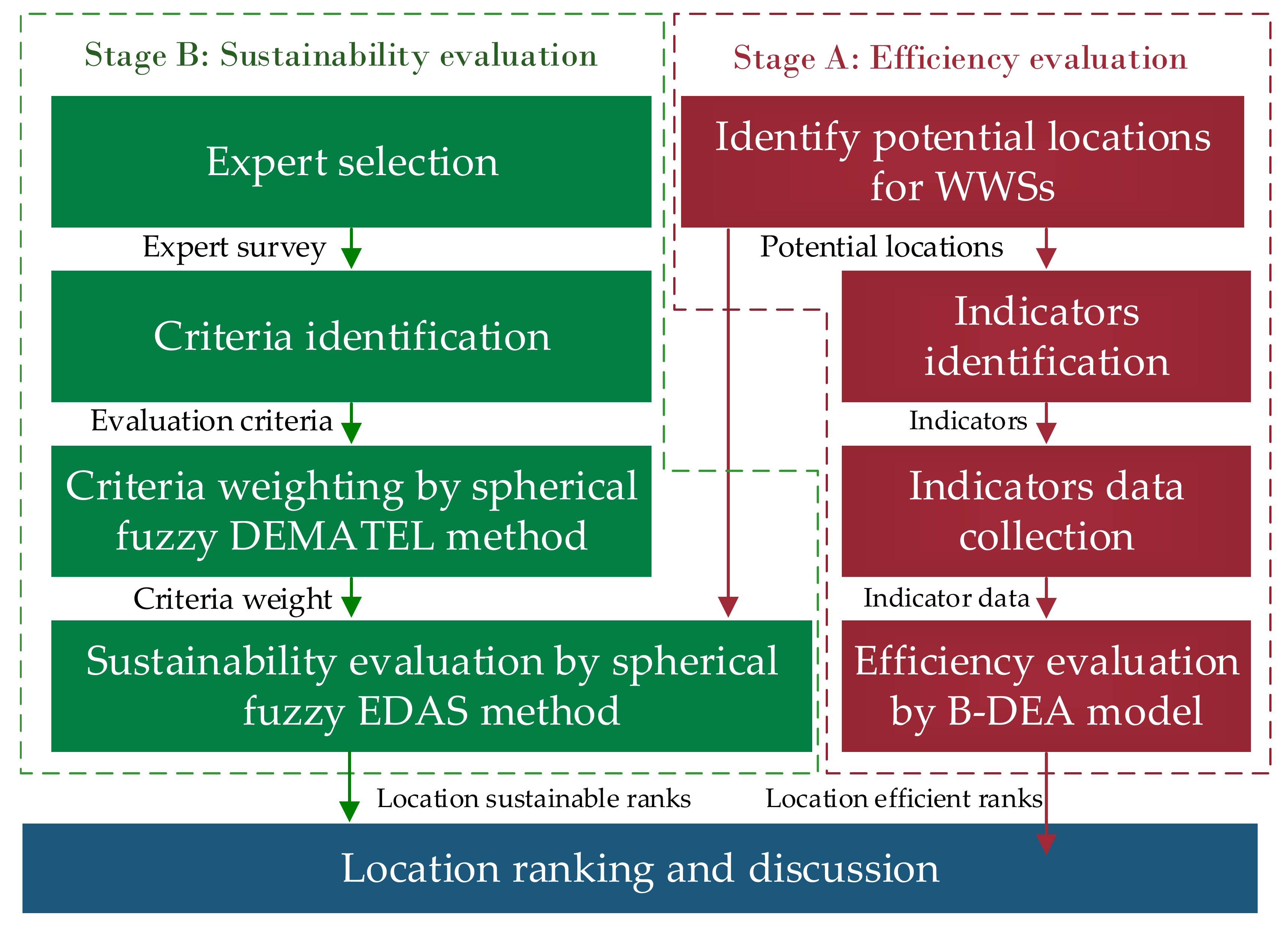
3. Methodology
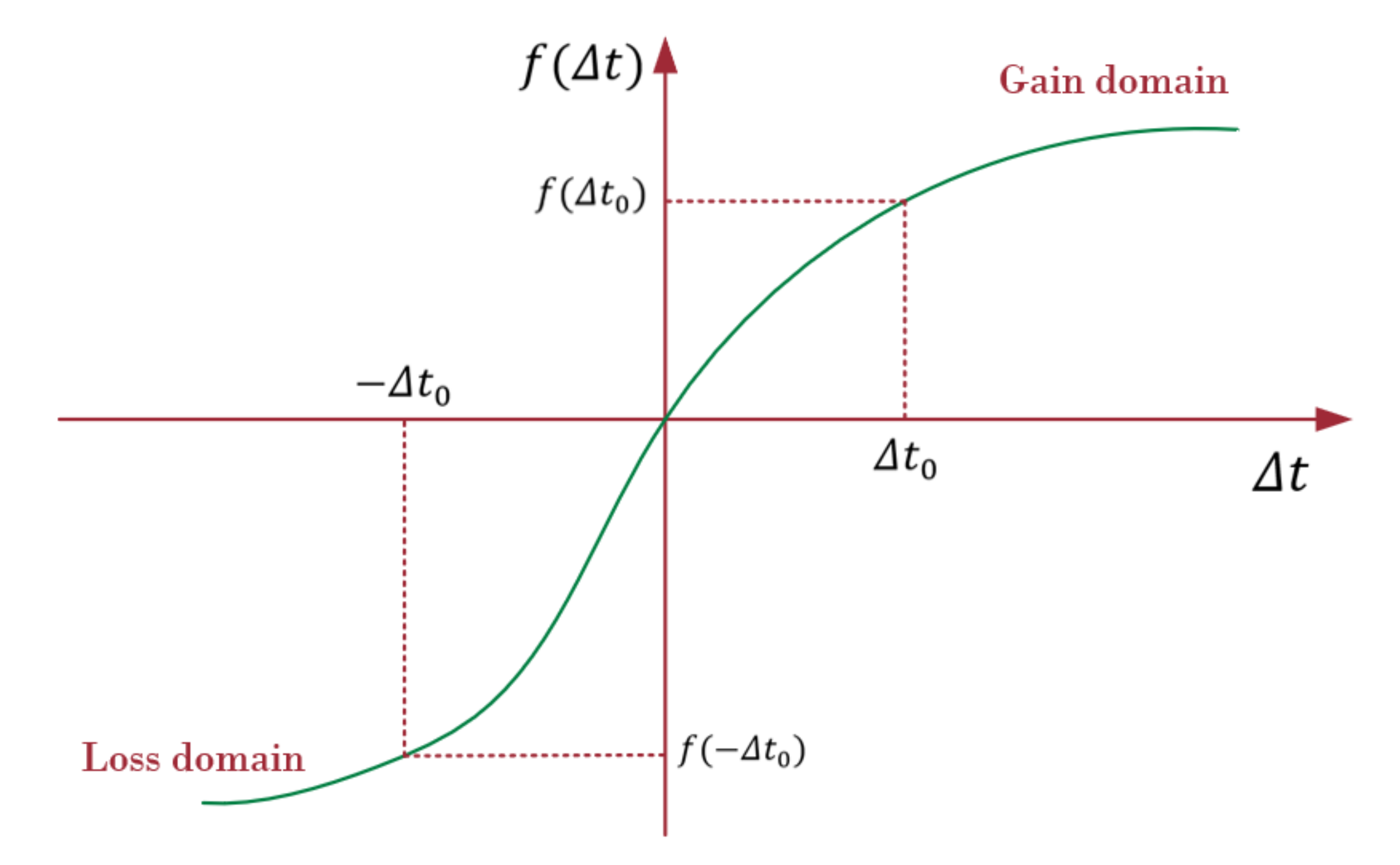
3.1. Behavioral Data Envelopment Analysis (B-DEA)
- Reference dependence: Individuals’ perceptions of gains and losses depend on a reference point.
- Loss aversion: Individuals’ sensitivity to losses is greater than to equal gains.
- Diminishing sensitivity: Individuals tend to be risk-seeking for losses and risk-averse for gains.
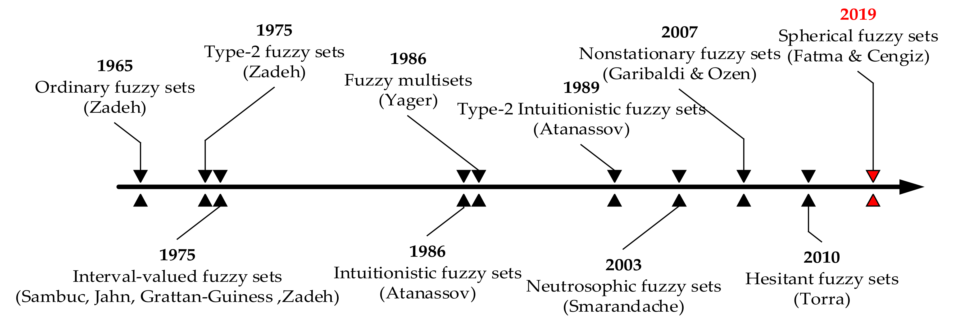
3.2. Spherical Fuzzy (SF) Sets
3.3. Spherical Fuzzy DEMATEL-EDAS Method
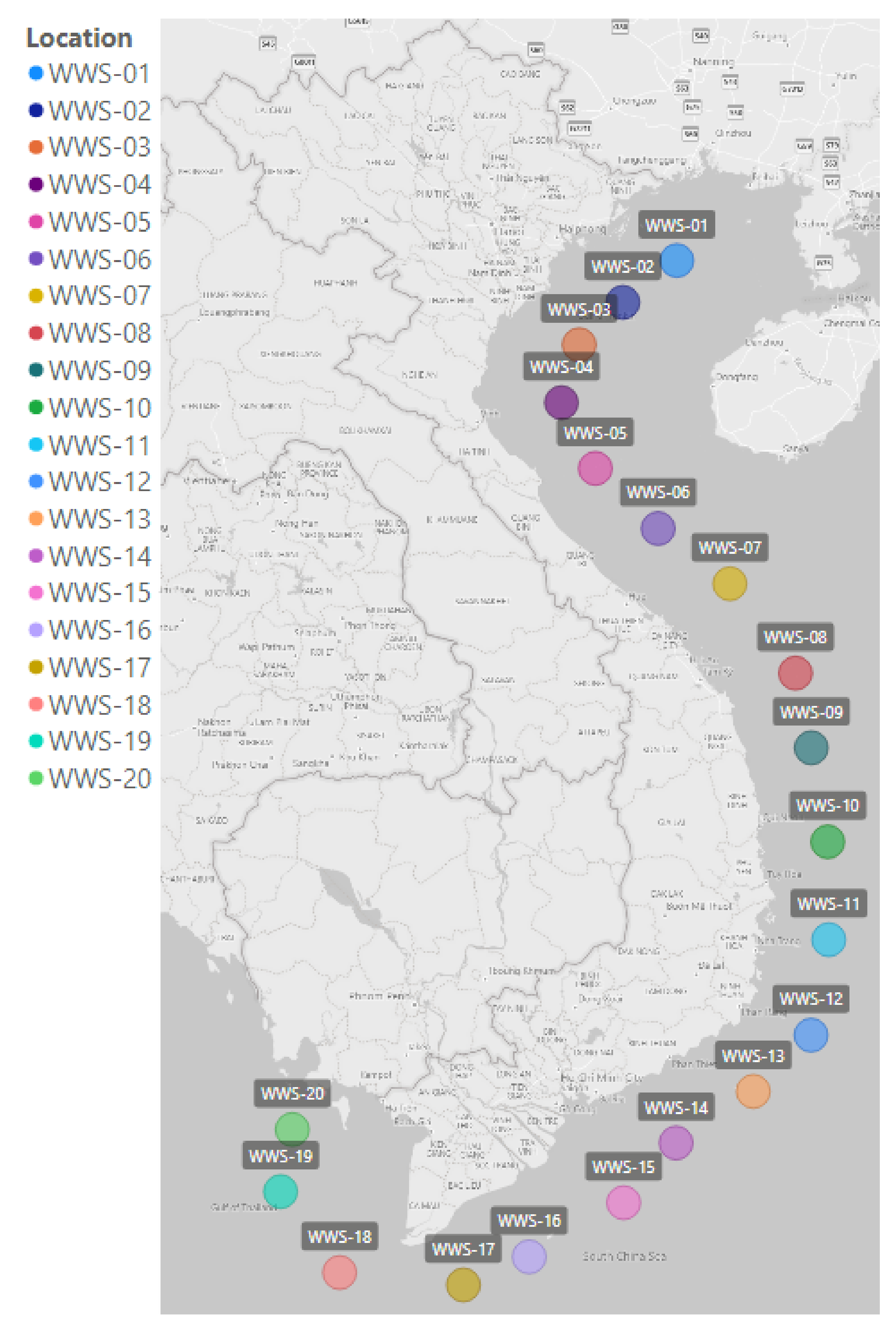
4. Case Study
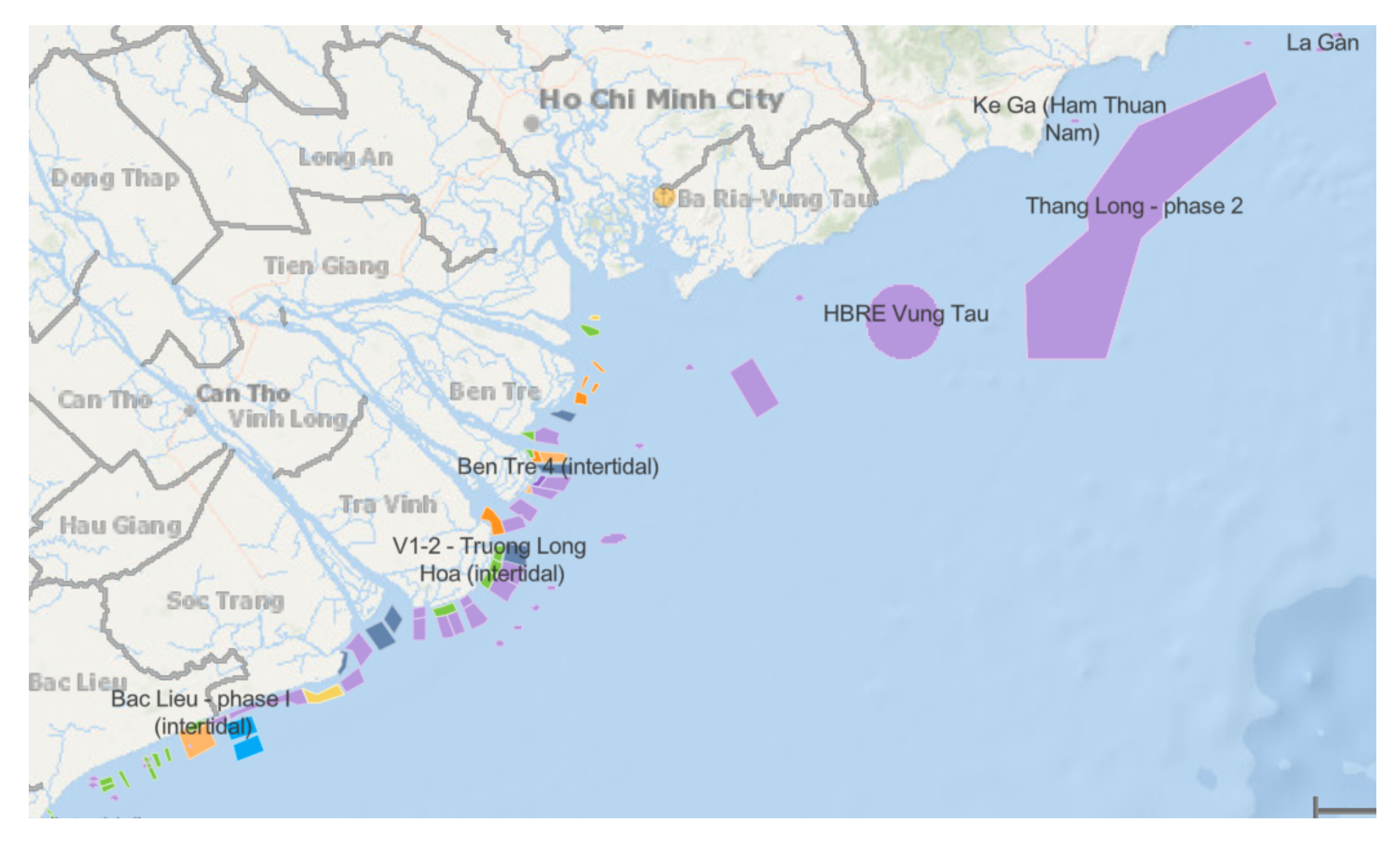
4.1. Location Identification
4.2. Stage A: Efficiency Evaluation by B-DEA Model
4.3. Stage B: Sustainability Evaluation by SF DEMATEL-EDAS Method
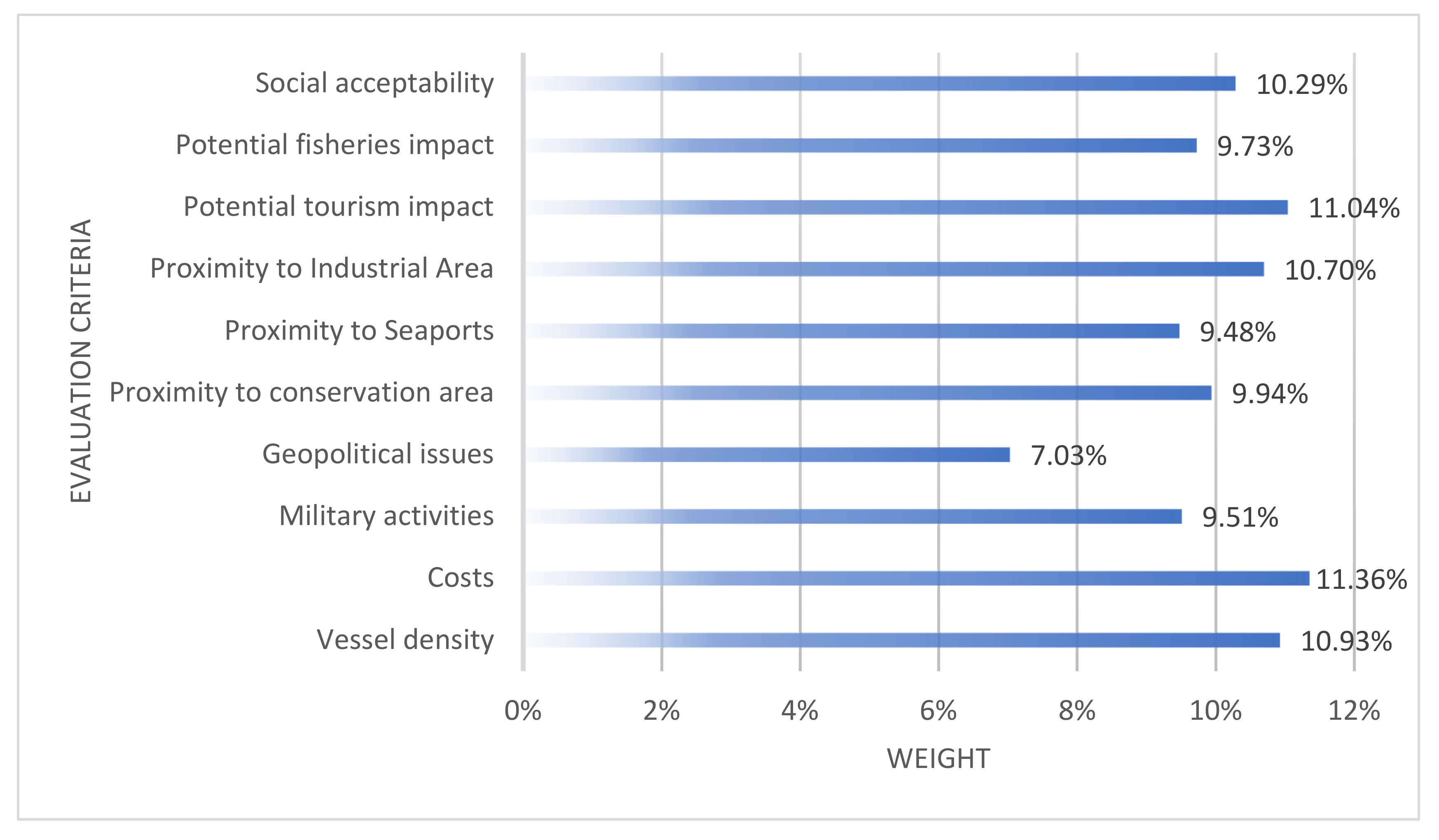
4.3.1. Evaluation Criteria Identification and Weighting
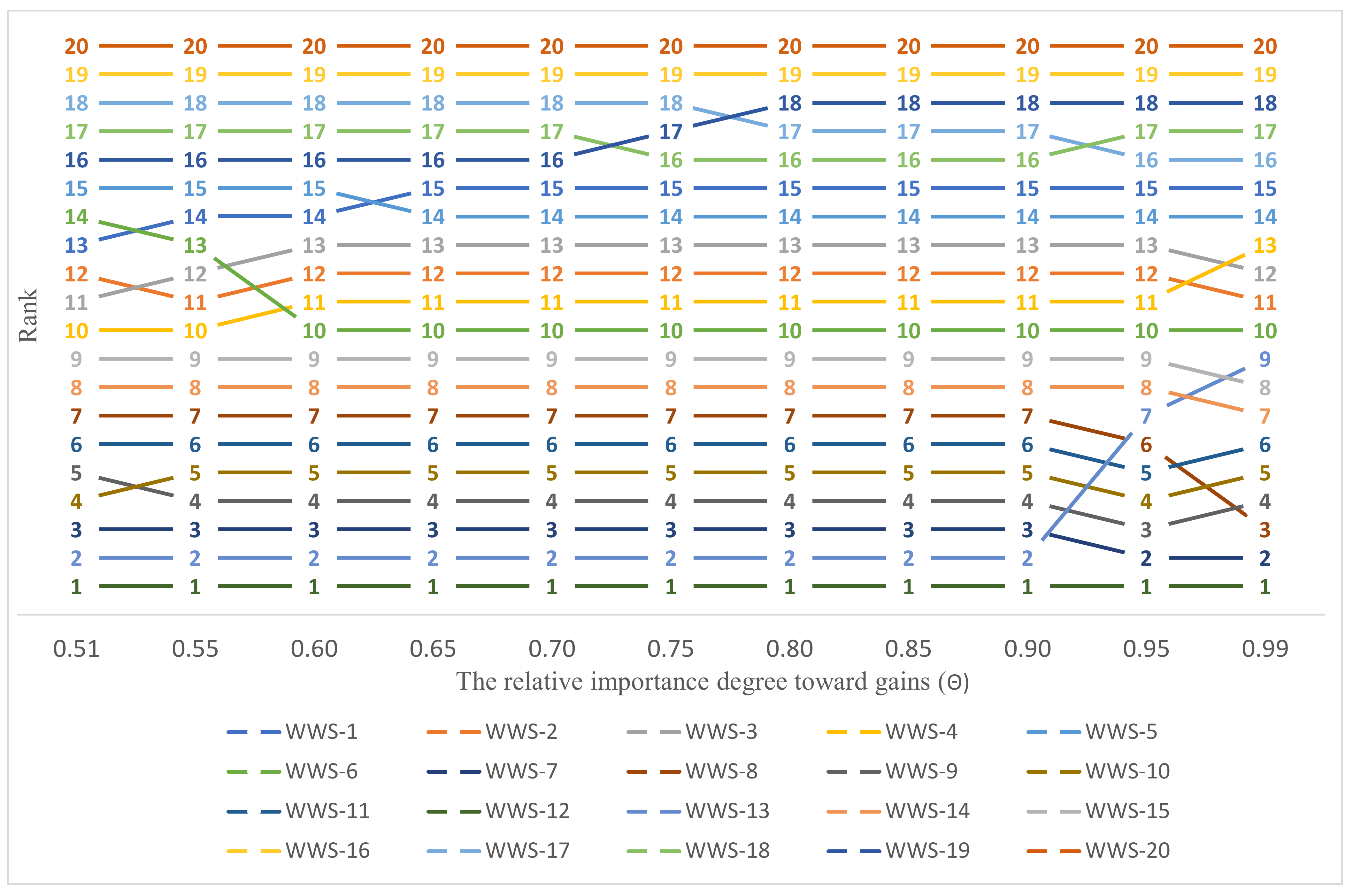
4.3.2. Sustainability Ranking
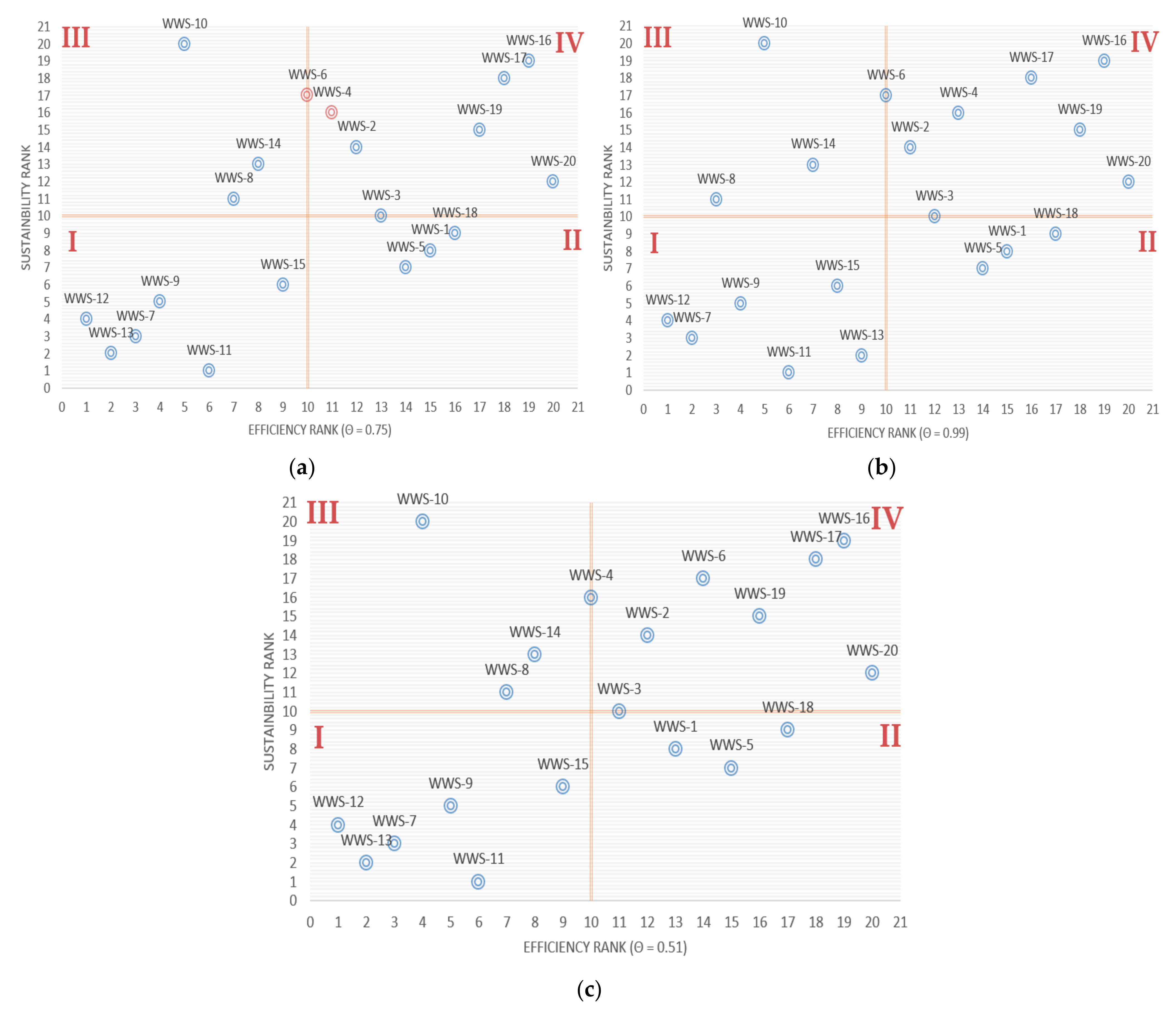
4.4. Dual-Side Analysis
4.5. Managerial Implications
5. Conclusions
5.1. Contributions and Findings
5.2. Limitations and Futher Research Recommendations
Author Contributions
Funding
Institutional Review Board Statement
Informed Consent Statement
Data Availability Statement
Acknowledgments
Conflicts of Interest
Appendix A

| Location | Latitude | Longitude | Location | Latitude | Longitude |
|---|---|---|---|---|---|
| WWS-1 | 20.591686 | 108.202101 | WWS-11 | 12.380291 | 110.120526 |
| WWS-2 | 20.097773 | 107.519992 | WWS-12 | 11.200562 | 109.896527 |
| WWS-3 | 19.594143 | 106.968776 | WWS-13 | 10.503389 | 109.167185 |
| WWS-4 | 18.903735 | 106.745225 | WWS-14 | 9.862731 | 108.192441 |
| WWS-5 | 18.116894 | 107.173398 | WWS-15 | 9.118867 | 107.530793 |
| WWS-6 | 17.393742 | 107.965662 | WWS-16 | 8.443364 | 106.337667 |
| WWS-7 | 16.727761 | 108.872040 | WWS-17 | 8.092894 | 105.506814 |
| WWS-8 | 15.643628 | 109.700175 | WWS-18 | 8.247452 | 103.944320 |
| WWS-9 | 14.734740 | 109.899698 | WWS-19 | 9.257728 | 103.199160 |
| WWS-10 | 13.583723 | 110.107265 | WWS-20 | 10.029545 | 103.346960 |
| Location | |||||||||||
|---|---|---|---|---|---|---|---|---|---|---|---|
| 0.51 | 0.55 | 0.60 | 0.65 | 0.70 | 0.75 | 0.80 | 0.85 | 0.90 | 0.95 | 0.99 | |
| WWS-1 | 0.027 | 0.071 | 0.126 | 0.182 | 0.237 | 0.293 | 0.394 | 0.495 | 0.596 | 0.696 | 0.797 |
| WWS-2 | 0.046 | 0.089 | 0.143 | 0.201 | 0.288 | 0.375 | 0.462 | 0.549 | 0.636 | 0.723 | 0.810 |
| WWS-3 | 0.046 | 0.089 | 0.143 | 0.201 | 0.288 | 0.375 | 0.462 | 0.549 | 0.636 | 0.723 | 0.810 |
| WWS-4 | 0.047 | 0.090 | 0.144 | 0.202 | 0.289 | 0.376 | 0.463 | 0.550 | 0.637 | 0.724 | 0.810 |
| WWS-5 | 0.016 | 0.061 | 0.117 | 0.198 | 0.286 | 0.373 | 0.461 | 0.548 | 0.635 | 0.723 | 0.810 |
| WWS-6 | 0.021 | 0.079 | 0.161 | 0.242 | 0.324 | 0.406 | 0.488 | 0.569 | 0.651 | 0.733 | 0.814 |
| WWS-7 | 0.102 | 0.160 | 0.234 | 0.307 | 0.380 | 0.453 | 0.526 | 0.600 | 0.673 | 0.746 | 0.819 |
| WWS-8 | 0.096 | 0.155 | 0.228 | 0.301 | 0.375 | 0.449 | 0.523 | 0.597 | 0.671 | 0.745 | 0.819 |
| WWS-9 | 0.100 | 0.159 | 0.232 | 0.306 | 0.379 | 0.452 | 0.526 | 0.599 | 0.673 | 0.746 | 0.819 |
| WWS-10 | 0.100 | 0.159 | 0.232 | 0.306 | 0.379 | 0.452 | 0.526 | 0.599 | 0.673 | 0.746 | 0.819 |
| WWS-11 | 0.099 | 0.158 | 0.231 | 0.305 | 0.378 | 0.452 | 0.525 | 0.599 | 0.672 | 0.746 | 0.819 |
| WWS-12 | 0.174 | 0.227 | 0.293 | 0.359 | 0.425 | 0.491 | 0.557 | 0.624 | 0.690 | 0.756 | 0.822 |
| WWS-13 | 0.128 | 0.184 | 0.254 | 0.324 | 0.394 | 0.464 | 0.534 | 0.605 | 0.675 | 0.745 | 0.815 |
| WWS-14 | 0.062 | 0.123 | 0.201 | 0.278 | 0.355 | 0.432 | 0.509 | 0.586 | 0.663 | 0.740 | 0.817 |
| WWS-15 | 0.061 | 0.122 | 0.200 | 0.277 | 0.354 | 0.431 | 0.508 | 0.586 | 0.663 | 0.740 | 0.817 |
| WWS-16 | 0.008 | 0.048 | 0.099 | 0.150 | 0.201 | 0.252 | 0.303 | 0.404 | 0.525 | 0.646 | 0.767 |
| WWS-17 | 0.009 | 0.050 | 0.101 | 0.152 | 0.203 | 0.254 | 0.347 | 0.457 | 0.567 | 0.677 | 0.787 |
| WWS-18 | 0.013 | 0.054 | 0.104 | 0.155 | 0.206 | 0.257 | 0.349 | 0.458 | 0.568 | 0.677 | 0.787 |
| WWS-19 | 0.014 | 0.055 | 0.105 | 0.156 | 0.207 | 0.257 | 0.308 | 0.407 | 0.529 | 0.650 | 0.771 |
| WWS-20 | 0.006 | 0.047 | 0.098 | 0.149 | 0.201 | 0.252 | 0.303 | 0.355 | 0.406 | 0.464 | 0.524 |
| Criteria | EC1 | EC2 | EC3 | EC4 | EC5 | EC6 | EC7 | EC8 | EC9 | EC10 |
|---|---|---|---|---|---|---|---|---|---|---|
| EC1 | NI | WI | NI | SI | WI | WI | WI | SI | MI | NI |
| EC2 | SI | NI | MI | NI | SI | SI | WI | NI | MI | SI |
| EC3 | NI | MI | NI | WI | NI | WI | WI | WI | SI | WI |
| EC4 | WI | NI | NI | NI | NI | WI | WI | MI | NI | WI |
| EC5 | SI | SI | NI | SI | NI | MI | MI | MI | SI | SI |
| EC6 | WI | MI | MI | SI | WI | NI | SI | SI | WI | MI |
| EC7 | MI | WI | SI | SI | MI | WI | NI | WI | MI | SI |
| EC8 | SI | MI | NI | MI | WI | WI | SI | NI | NI | SI |
| EC9 | NI | SI | MI | WI | SI | NI | SI | NI | NI | SI |
| EC10 | MI | WI | MI | SI | MI | SI | MI | MI | WI | NI |
| Criteria | R | C | Prominence | Relation | Weight | ||
|---|---|---|---|---|---|---|---|
| EC1 | (0.981, 0.060, 0.193) | 0.639 | (0.972, 0.090, 0.236) | 0.562 | 1.201 | 0.077 | 0.109 |
| EC2 | (0.975, 0.086, 0.223) | 0.584 | (0.984, 0.058, 0.178) | 0.664 | 1.248 | −0.080 | 0.114 |
| EC3 | (0.960, 0.126, 0.281) | 0.484 | (0.972, 0.093, 0.237) | 0.561 | 1.045 | −0.077 | 0.095 |
| EC4 | (0.847, 0.311, 0.530) | 0.148 | (0.980, 0.074, 0.200) | 0.624 | 0.773 | −0.476 | 0.070 |
| EC5 | (0.964, 0.106, 0.264) | 0.516 | (0.974, 0.090, 0.227) | 0.577 | 1.092 | −0.061 | 0.099 |
| EC6 | (0.968, 0.107, 0.252) | 0.534 | (0.963, 0.104, 0.270) | 0.508 | 1.042 | 0.026 | 0.095 |
| EC7 | (0.977, 0.076, 0.212) | 0.605 | (0.973, 0.080, 0.232) | 0.571 | 1.176 | 0.034 | 0.107 |
| EC8 | (0.993, 0.031, 0.122) | 0.767 | (0.953, 0.145, 0.303) | 0.447 | 1.214 | 0.319 | 0.110 |
| EC9 | (0.974, 0.087, 0.228) | 0.576 | (0.961, 0.116, 0.277) | 0.493 | 1.069 | 0.082 | 0.097 |
| EC10 | (0.973, 0.083, 0.229) | 0.576 | (0.970, 0.086, 0.242) | 0.555 | 1.131 | 0.021 | 0.103 |
| Location | EC1 | EC2 | EC3 | EC4 | EC5 | EC6 | EC7 | EC8 | EC9 | EC10 |
|---|---|---|---|---|---|---|---|---|---|---|
| WWS-1 | M | L | M | SH | VH | H | SH | M | L | VHI |
| WWS-2 | H | L | L | SH | AL | H | L | M | SH | AL |
| WWS-3 | AH | VH | VL | H | AL | M | VL | VL | H | AH |
| WWS-4 | VH | VH | SH | L | VL | AL | VH | H | H | H |
| WWS-5 | SH | SH | L | M | VL | SH | AH | SL | VH | AH |
| WWS-6 | SH | SH | AH | VL | H | SH | SH | AH | H | SH |
| WWS-7 | AH | VL | H | VH | SL | VL | M | VH | AH | SL |
| WWS-8 | VL | VL | VL | AH | M | AH | AL | SL | VH | H |
| WWS-9 | AL | AH | L | H | H | SH | SL | SL | H | VH |
| WWS-10 | AL | SH | AH | VH | VH | M | H | M | VL | M |
| WWS-11 | SH | VL | VL | L | VH | L | AH | VH | VH | SL |
| WWS-12 | H | SH | L | H | L | AL | VH | SH | VL | VL |
| WWS-13 | VH | H | AH | VH | M | SL | VH | VL | M | SL |
| WWS-14 | VH | VH | AL | SL | SL | M | AH | AL | SL | M |
| WWS-15 | AH | AL | M | AH | VH | SL | SL | VL | AH | L |
| WWS-16 | SH | AL | VH | VH | VL | SL | L | SL | VL | H |
| WWS-17 | L | M | VL | VL | SL | AH | SH | H | AL | VH |
| WWS-18 | SL | AH | VH | AH | SL | VL | VL | AL | M | L |
| WWS-19 | SL | AL | L | L | L | AL | VL | VL | H | AL |
| WWS-20 | SH | AH | H | VL | AH | SL | M | SL | VL | AL |
| Location | EC1 | EC2 | EC3 | EC4 | EC5 |
| WWS-1 | (0.73, 0.28, 0.31) | (0.66, 0.37, 0.29) | (0.70, 0.33, 0.33) | (0.62, 0.41, 0.33) | (0.66, 0.35, 0.31) |
| WWS-2 | (0.58, 0.46, 0.30) | (0.56, 0.46, 0.36) | (0.40, 0.64, 0.31) | (0.57, 0.47, 0.35) | (0.57, 0.48, 0.32) |
| WWS-3 | (0.66, 0.37, 0.29) | (0.68, 0.33, 0.31) | (0.50, 0.56, 0.34) | (0.74, 0.27, 0.30) | (0.66, 0.38, 0.27) |
| WWS-4 | (0.61, 0.42, 0.30) | (0.69, 0.33, 0.25) | (0.61, 0.44, 0.25) | (0.68, 0.35, 0.27) | (0.56, 0.49, 0.31) |
| WWS-5 | (0.63, 0.42, 0.27) | (0.62, 0.41, 0.31) | (0.67, 0.37, 0.27) | (0.72, 0.29, 0.28) | (0.60, 0.45, 0.26) |
| WWS-6 | (0.57, 0.46, 0.31) | (0.63, 0.39, 0.31) | (0.70, 0.33, 0.29) | (0.70, 0.35, 0.24) | (0.68, 0.35, 0.28) |
| WWS-7 | (0.79, 0.22, 0.24) | (0.52, 0.53, 0.33) | (0.66, 0.37, 0.28) | (0.66, 0.36, 0.30) | (0.62, 0.40, 0.34) |
| WWS-8 | (0.63, 0.40, 0.31) | (0.61, 0.43, 0.31) | (0.57, 0.48, 0.29) | (0.68, 0.36, 0.26) | (0.55, 0.51, 0.30) |
| WWS-9 | (0.54, 0.49, 0.37) | (0.67, 0.37, 0.24) | (0.64, 0.39, 0.31) | (0.65, 0.39, 0.27) | (0.65, 0.38, 0.31) |
| WWS-10 | (0.51, 0.53, 0.31) | (0.49, 0.54, 0.34) | (0.59, 0.44, 0.36) | (0.49, 0.56, 0.31) | (0.71, 0.33, 0.24) |
| WWS-11 | (0.77, 0.25, 0.21) | (0.55, 0.50, 0.31) | (0.64, 0.39, 0.30) | (0.65, 0.38, 0.29) | (0.64, 0.40, 0.28) |
| WWS-12 | (0.67, 0.35, 0.32) | (0.62, 0.41, 0.32) | (0.64, 0.39, 0.28) | (0.70, 0.32, 0.24) | (0.69, 0.35, 0.23) |
| WWS-13 | (0.70, 0.32, 0.31) | (0.71, 0.33, 0.20) | (0.64, 0.38, 0.29) | (0.67, 0.37, 0.26) | (0.48, 0.53, 0.40) |
| WWS-14 | (0.66, 0.36, 0.29) | (0.70, 0.32, 0.28) | (0.60, 0.44, 0.28) | (0.63, 0.40, 0.28) | (0.61, 0.42, 0.35) |
| WWS-15 | (0.76, 0.26, 0.20) | (0.51, 0.53, 0.29) | (0.68, 0.35, 0.28) | (0.72, 0.31, 0.24) | (0.57, 0.47, 0.35) |
| WWS-16 | (0.69, 0.33, 0.28) | (0.59, 0.44, 0.39) | (0.69, 0.34, 0.28) | (0.73, 0.30, 0.22) | (0.58, 0.45, 0.34) |
| WWS-17 | (0.60, 0.44, 0.30) | (0.60, 0.44, 0.32) | (0.66, 0.40, 0.22) | (0.60, 0.45, 0.28) | (0.46, 0.57, 0.37) |
| WWS-18 | (0.55, 0.47, 0.37) | (0.56, 0.49, 0.28) | (0.68, 0.35, 0.31) | (0.67, 0.36, 0.30) | (0.79, 0.22, 0.20) |
| WWS-19 | (0.55, 0.48, 0.34) | (0.58, 0.46, 0.31) | (0.42, 0.60, 0.34) | (0.78, 0.23, 0.21) | (0.58, 0.47, 0.28) |
| WWS-20 | (0.67, 0.35, 0.31) | (0.63, 0.39, 0.35) | (0.74, 0.29, 0.20) | (0.63, 0.4, 0.28) | (0.66, 0.38, 0.28) |
| Location | EC6 | EC7 | EC8 | EC9 | EC10 |
| WWS-1 | (0.64, 0.38, 0.30) | (0.65, 0.38, 0.31) | (0.51, 0.54, 0.32) | (0.53, 0.48, 0.39) | (0.75, 0.27, 0.20) |
| WWS-2 | (0.67, 0.34, 0.35) | (0.69, 0.33, 0.28) | (0.64, 0.39, 0.28) | (0.64, 0.39, 0.32) | (0.70, 0.35, 0.20) |
| WWS-3 | (0.59, 0.46, 0.30) | (0.62, 0.43, 0.30) | (0.63, 0.39, 0.32) | (0.60, 0.45, 0.26) | (0.53, 0.53, 0.29) |
| WWS-4 | (0.50, 0.56, 0.29) | (0.57, 0.45, 0.36) | (0.63, 0.40, 0.30) | (0.52, 0.51, 0.38) | (0.59, 0.45, 0.33) |
| WWS-5 | (0.66, 0.35, 0.33) | (0.62, 0.44, 0.22) | (0.49, 0.55, 0.33) | (0.51, 0.53, 0.32) | (0.65, 0.39, 0.29) |
| WWS-6 | (0.68, 0.35, 0.32) | (0.47, 0.55, 0.37) | (0.60, 0.43, 0.34) | (0.57, 0.47, 0.28) | (0.57, 0.46, 0.35) |
| WWS-7 | (0.60, 0.45, 0.27) | (0.59, 0.45, 0.32) | (0.79, 0.22, 0.18) | (0.66, 0.36, 0.32) | (0.51, 0.50, 0.36) |
| WWS-8 | (0.61, 0.44, 0.25) | (0.64, 0.40, 0.28) | (0.52, 0.52, 0.30) | (0.67, 0.36, 0.31) | (0.58, 0.47, 0.26) |
| WWS-9 | (0.74, 0.28, 0.24) | (0.62, 0.41, 0.29) | (0.57, 0.46, 0.34) | (0.65, 0.38, 0.27) | (0.72, 0.31, 0.23) |
| WWS-10 | (0.56, 0.46, 0.38) | (0.52, 0.50, 0.37) | (0.6, 0.43, 0.32) | (0.63, 0.40, 0.29) | (0.58, 0.47, 0.31) |
| WWS-11 | (0.68, 0.35, 0.26) | (0.71, 0.32, 0.27) | (0.63, 0.40, 0.30) | (0.70, 0.33, 0.26) | (0.68, 0.35, 0.25) |
| WWS-12 | (0.57, 0.49, 0.27) | (0.68, 0.34, 0.24) | (0.49, 0.54, 0.37) | (0.57, 0.48, 0.28) | (0.27, 0.76, 0.28) |
| WWS-13 | (0.67, 0.36, 0.28) | (0.71, 0.33, 0.24) | (0.70, 0.33, 0.26) | (0.58, 0.47, 0.32) | (0.64, 0.39, 0.33) |
| WWS-14 | (0.59, 0.44, 0.39) | (0.69, 0.34, 0.24) | (0.55, 0.48, 0.36) | (0.76, 0.27, 0.23) | (0.53, 0.49, 0.36) |
| WWS-15 | (0.59, 0.44, 0.30) | (0.72, 0.31, 0.24) | (0.52, 0.51, 0.35) | (0.65, 0.38, 0.25) | (0.55, 0.49, 0.35) |
| WWS-16 | (0.58, 0.44, 0.31) | (0.47, 0.56, 0.36) | (0.51, 0.52, 0.34) | (0.62, 0.41, 0.34) | (0.52, 0.52, 0.35) |
| WWS-17 | (0.70, 0.35, 0.21) | (0.54, 0.47, 0.41) | (0.53, 0.51, 0.35) | (0.53, 0.52, 0.30) | (0.63, 0.39, 0.34) |
| WWS-18 | (0.57, 0.46, 0.33) | (0.59, 0.45, 0.30) | (0.65, 0.42, 0.23) | (0.57, 0.46, 0.36) | (0.64, 0.39, 0.30) |
| WWS-19 | (0.61, 0.42, 0.30) | (0.47, 0.60, 0.28) | (0.61, 0.42, 0.30) | (0.60, 0.44, 0.32) | (0.55, 0.48, 0.32) |
| WWS-20 | (0.57, 0.47, 0.32) | (0.64, 0.39, 0.28) | (0.61, 0.43, 0.34) | (0.49, 0.55, 0.34) | (0.53, 0.53, 0.28) |
| Criteria | EC1 | EC2 | EC3 | EC4 | EC5 |
| Average solution | (0.66, 0.37, 0.30) | (0.62, 0.42, 0.31) | (0.63, 0.41, 0.29) | (0.67, 0.36, 0.28) | (0.63, 0.41, 0.30) |
| Criteria | EC6 | EC7 | EC8 | EC9 | EC10 |
| Average solution | (0.62, 0.41, 0.31) | (0.62, 0.42, 0.30) | (0.60, 0.44, 0.31) | (0.61, 0.43, 0.31) | (0.60, 0.44, 0.30) |
| Location | EC1 | EC2 | EC3 | EC4 | EC5 | EC6 | EC7 | EC8 | EC9 | EC10 |
|---|---|---|---|---|---|---|---|---|---|---|
| WWS-1 | 0.182 | 0.140 | 0.135 | 0.093 | 0.128 | 0.126 | 0.120 | 0.083 | 0.028 | 0.315 |
| WWS-2 | 0.106 | 0.052 | 0.122 | 0.062 | 0.090 | 0.101 | 0.171 | 0.142 | 0.103 | 0.267 |
| WWS-3 | 0.145 | 0.137 | 0.076 | 0.192 | 0.165 | 0.107 | 0.119 | 0.108 | 0.153 | 0.114 |
| WWS-4 | 0.110 | 0.197 | 0.160 | 0.178 | 0.092 | 0.115 | 0.055 | 0.115 | 0.037 | 0.082 |
| WWS-5 | 0.149 | 0.106 | 0.167 | 0.195 | 0.147 | 0.112 | 0.210 | 0.071 | 0.081 | 0.145 |
| WWS-6 | 0.089 | 0.109 | 0.162 | 0.221 | 0.165 | 0.125 | 0.044 | 0.080 | 0.117 | 0.058 |
| WWS-7 | 0.304 | 0.075 | 0.152 | 0.131 | 0.083 | 0.135 | 0.091 | 0.372 | 0.117 | 0.044 |
| WWS-8 | 0.111 | 0.103 | 0.114 | 0.191 | 0.104 | 0.165 | 0.145 | 0.094 | 0.130 | 0.150 |
| WWS-9 | 0.043 | 0.202 | 0.115 | 0.161 | 0.120 | 0.249 | 0.126 | 0.067 | 0.161 | 0.243 |
| WWS-10 | 0.093 | 0.059 | 0.059 | 0.091 | 0.223 | 0.038 | 0.040 | 0.094 | 0.135 | 0.100 |
| WWS-11 | 0.306 | 0.090 | 0.124 | 0.135 | 0.139 | 0.187 | 0.196 | 0.121 | 0.198 | 0.191 |
| WWS-12 | 0.128 | 0.098 | 0.137 | 0.219 | 0.227 | 0.142 | 0.206 | 0.041 | 0.129 | 0.226 |
| WWS-13 | 0.152 | 0.271 | 0.129 | 0.181 | 0.023 | 0.156 | 0.231 | 0.196 | 0.089 | 0.100 |
| WWS-14 | 0.141 | 0.177 | 0.133 | 0.138 | 0.075 | 0.045 | 0.210 | 0.051 | 0.280 | 0.045 |
| WWS-15 | 0.326 | 0.104 | 0.164 | 0.238 | 0.062 | 0.102 | 0.233 | 0.052 | 0.180 | 0.059 |
| WWS-16 | 0.170 | 0.042 | 0.173 | 0.261 | 0.067 | 0.095 | 0.049 | 0.063 | 0.084 | 0.056 |
| WWS-17 | 0.109 | 0.098 | 0.225 | 0.131 | 0.047 | 0.258 | 0.021 | 0.053 | 0.097 | 0.084 |
| WWS-18 | 0.043 | 0.120 | 0.136 | 0.137 | 0.354 | 0.074 | 0.107 | 0.213 | 0.057 | 0.122 |
| WWS-19 | 0.066 | 0.102 | 0.079 | 0.325 | 0.124 | 0.111 | 0.141 | 0.113 | 0.090 | 0.083 |
| WWS-20 | 0.130 | 0.078 | 0.305 | 0.140 | 0.158 | 0.086 | 0.139 | 0.080 | 0.062 | 0.127 |
| Average solution | 0.135 | 0.108 | 0.129 | 0.164 | 0.120 | 0.113 | 0.118 | 0.099 | 0.106 | 0.110 |
| Location | EC1 | EC2 | EC3 | EC4 | EC5 | EC6 | EC7 | EC8 | EC9 | EC10 |
|---|---|---|---|---|---|---|---|---|---|---|
| WWS-1 | 0.346 | 0.301 | 0.053 | 0 | 0.063 | 0.115 | 0.022 | 0 | 0 | 1.866 |
| WWS-2 | 0 | 0 | 0 | 0 | 0 | 0 | 0.449 | 0.432 | 0 | 1.43 |
| WWS-3 | 0.075 | 0.277 | 0 | 0.169 | 0.371 | 0 | 0.011 | 0.088 | 0.449 | 0.042 |
| WWS-4 | 0 | 0.833 | 0.248 | 0.083 | 0 | 0.02 | 0 | 0.159 | 0 | 0 |
| WWS-5 | 0.1 | 0 | 0.296 | 0.191 | 0.224 | 0 | 0.779 | 0 | 0 | 0.319 |
| WWS-6 | 0 | 0.013 | 0.26 | 0.348 | 0.368 | 0.108 | 0 | 0 | 0.101 | 0 |
| WWS-7 | 1.251 | 0 | 0.182 | 0 | 0 | 0.197 | 0 | 2.749 | 0.107 | 0 |
| WWS-8 | 0 | 0 | 0 | 0.166 | 0 | 0.464 | 0.23 | 0 | 0.227 | 0.366 |
| WWS-9 | 0 | 0.876 | 0 | 0 | 0 | 1.208 | 0.072 | 0 | 0.516 | 1.213 |
| WWS-10 | 0 | 0 | 0 | 0 | 0.859 | 0 | 0 | 0 | 0.279 | 0 |
| WWS-11 | 1.265 | 0 | 0 | 0 | 0.154 | 0.663 | 0.664 | 0.217 | 0.87 | 0.742 |
| WWS-12 | 0 | 0 | 0.066 | 0.334 | 0.892 | 0.262 | 0.748 | 0 | 0.219 | 1.058 |
| WWS-13 | 0.127 | 1.522 | 0.003 | 0.107 | 0 | 0.381 | 0.964 | 0.977 | 0 | 0 |
| WWS-14 | 0.046 | 0.648 | 0.032 | 0 | 0 | 0 | 0.778 | 0 | 1.648 | 0 |
| WWS-15 | 1.413 | 0 | 0.278 | 0.452 | 0 | 0 | 0.979 | 0 | 0.699 | 0 |
| WWS-16 | 0.256 | 0 | 0.342 | 0.594 | 0 | 0 | 0 | 0 | 0 | 0 |
| WWS-17 | 0 | 0 | 0.752 | 0 | 0 | 1.291 | 0 | 0 | 0 | 0 |
| WWS-18 | 0 | 0.112 | 0.057 | 0 | 1.942 | 0 | 0 | 1.151 | 0 | 0.113 |
| WWS-19 | 0 | 0 | 0 | 0.985 | 0.035 | 0 | 0.199 | 0.137 | 0 | 0 |
| WWS-20 | 0 | 0 | 1.369 | 0 | 0.314 | 0 | 0.181 | 0 | 0 | 0.159 |
| Location | EC1 | EC2 | EC3 | EC4 | EC5 | EC6 | EC7 | EC8 | EC9 | EC10 |
|---|---|---|---|---|---|---|---|---|---|---|
| WWS-1 | 0 | 0 | 0 | 0.43 | 0 | 0 | 0 | 0.16 | 0.74 | 0 |
| WWS-2 | 0.215 | 0.52 | 0.048 | 0.624 | 0.248 | 0.106 | 0 | 0 | 0.028 | 0 |
| WWS-3 | 0 | 0 | 0.405 | 0 | 0 | 0.049 | 0 | 0 | 0 | 0 |
| WWS-4 | 0.188 | 0 | 0 | 0 | 0.237 | 0 | 0.535 | 0 | 0.647 | 0.249 |
| WWS-5 | 0 | 0.015 | 0 | 0 | 0 | 0.006 | 0 | 0.286 | 0.235 | 0 |
| WWS-6 | 0.342 | 0 | 0 | 0 | 0 | 0 | 0.626 | 0.192 | 0 | 0.47 |
| WWS-7 | 0 | 0.305 | 0 | 0.203 | 0.306 | 0 | 0.231 | 0 | 0 | 0.604 |
| WWS-8 | 0.181 | 0.043 | 0.117 | 0 | 0.136 | 0 | 0 | 0.048 | 0 | 0 |
| WWS-9 | 0.682 | 0 | 0.105 | 0.016 | 0.006 | 0 | 0 | 0.328 | 0 | 0 |
| WWS-10 | 0.309 | 0.448 | 0.538 | 0.443 | 0 | 0.663 | 0.658 | 0.055 | 0 | 0.088 |
| WWS-11 | 0 | 0.168 | 0.036 | 0.176 | 0 | 0 | 0 | 0 | 0 | 0 |
| WWS-12 | 0.053 | 0.087 | 0 | 0 | 0 | 0 | 0 | 0.583 | 0 | 0 |
| WWS-13 | 0 | 0 | 0 | 0 | 0.807 | 0 | 0 | 0 | 0.155 | 0.092 |
| WWS-14 | 0 | 0 | 0 | 0.159 | 0.379 | 0.605 | 0 | 0.487 | 0 | 0.588 |
| WWS-15 | 0 | 0.035 | 0 | 0 | 0.483 | 0.09 | 0 | 0.473 | 0 | 0.46 |
| WWS-16 | 0 | 0.614 | 0 | 0 | 0.441 | 0.16 | 0.588 | 0.363 | 0.203 | 0.491 |
| WWS-17 | 0.191 | 0.089 | 0 | 0.2 | 0.605 | 0 | 0.818 | 0.462 | 0.087 | 0.239 |
| WWS-18 | 0.682 | 0 | 0 | 0.165 | 0 | 0.339 | 0.09 | 0 | 0.462 | 0 |
| WWS-19 | 0.515 | 0.049 | 0.385 | 0 | 0 | 0.017 | 0 | 0 | 0.147 | 0.24 |
| WWS-20 | 0.038 | 0.272 | 0 | 0.146 | 0 | 0.239 | 0 | 0.194 | 0.413 | 0 |
| Location | Sustainability Aspect | ||||||||||
|---|---|---|---|---|---|---|---|---|---|---|---|
| 0.55 | 0.60 | 0.65 | 0.70 | 0.75 | 0.80 | 0.85 | 0.90 | 0.95 | 1.00 | ||
| WWS-1 | 8 | 14 | 14 | 15 | 15 | 15 | 15 | 15 | 15 | 15 | 15 |
| WWS-2 | 14 | 11 | 12 | 12 | 12 | 12 | 12 | 12 | 12 | 12 | 11 |
| WWS-3 | 10 | 12 | 13 | 13 | 13 | 13 | 13 | 13 | 13 | 13 | 12 |
| WWS-4 | 16 | 10 | 11 | 11 | 11 | 11 | 11 | 11 | 11 | 11 | 13 |
| WWS-5 | 7 | 15 | 15 | 14 | 14 | 14 | 14 | 14 | 14 | 14 | 14 |
| WWS-6 | 17 | 13 | 10 | 10 | 10 | 10 | 10 | 10 | 10 | 10 | 10 |
| WWS-7 | 3 | 3 | 3 | 3 | 3 | 3 | 3 | 3 | 3 | 2 | 2 |
| WWS-8 | 11 | 7 | 7 | 7 | 7 | 7 | 7 | 7 | 7 | 6 | 3 |
| WWS-9 | 5 | 4 | 4 | 4 | 4 | 4 | 4 | 4 | 4 | 3 | 4 |
| WWS-10 | 20 | 5 | 5 | 5 | 5 | 5 | 5 | 5 | 5 | 4 | 5 |
| WWS-11 | 1 | 6 | 6 | 6 | 6 | 6 | 6 | 6 | 6 | 5 | 6 |
| WWS-12 | 4 | 1 | 1 | 1 | 1 | 1 | 1 | 1 | 1 | 1 | 1 |
| WWS-13 | 2 | 2 | 2 | 2 | 2 | 2 | 2 | 2 | 2 | 7 | 9 |
| WWS-14 | 13 | 8 | 8 | 8 | 8 | 8 | 8 | 8 | 8 | 8 | 7 |
| WWS-15 | 6 | 9 | 9 | 9 | 9 | 9 | 9 | 9 | 9 | 9 | 8 |
| WWS-16 | 19 | 19 | 19 | 19 | 19 | 19 | 19 | 19 | 19 | 19 | 19 |
| WWS-17 | 18 | 18 | 18 | 18 | 18 | 18 | 17 | 17 | 17 | 16 | 16 |
| WWS-18 | 9 | 17 | 17 | 17 | 17 | 16 | 16 | 16 | 16 | 17 | 17 |
| WWS-19 | 15 | 16 | 16 | 16 | 16 | 17 | 18 | 18 | 18 | 18 | 18 |
| WWS-20 | 12 | 20 | 20 | 20 | 20 | 20 | 20 | 20 | 20 | 20 | 20 |
References
- International Energy Agency. Renewables 2021—Analysis and Forecast to 2026; International Energy Agency: Paris, France, 2021. [Google Scholar]
- Gao, Q.; Ertugrul, N.; Ding, B.; Negnevitsky, M. Offshore Wind, Wave and Integrated Energy Conversion Systems: A Review and Future. In Proceeding of the Australasian Universities Power Engineering Conference, Hobart, TAS, Australia, 29 November–2 December 2020; pp. 1–6. [Google Scholar]
- Yu-Hsien, L.; Ming-Chung, F. An Integrated Approach for Site Selection of Offshore Wind-Wave Power Production. IEEE J. Ocean. Eng. 2012, 37, 740–755. [Google Scholar] [CrossRef]
- Cheng, Z.; Wen, T.R.; Ong, M.C.; Wang, K. Power Performance and Dynamic Responses of a Combined Floating Vertical Axis Wind Turbine and Wave Energy Converter Concept. Energy 2019, 171, 190–204. [Google Scholar] [CrossRef]
- Peiffer, A.; Roddier, D.; Aubault, A. Design of a Point Absorber inside the WindFloat Structure. In Proceedings of the ASME 2011 30th International Conference on Ocean, Offshore and Arctic Engineering, Rotterdam, The Netherlands, 19–24 June 2011. [Google Scholar]
- Aubault, A.; Alves, M.; Sarmento, A.N.; Roddier, D.; Peiffer, A. Modeling of an Oscillating Water Column on the Floating Foundation WindFloat. In Proceedings of the ASME 2011 30th International Conference on Ocean, Offshore and Arctic Engineering, Rotterdam, The Netherlands, 19–24 June 2011. [Google Scholar]
- Perez, C.; Iglesias, G. Integration of Wave Energy Converters and Offshore Windmills. In Proceedings of the 4th International Conference on Ocean Energy, Dublin, Ireland, 17 October 2012. [Google Scholar]
- Shao, M.; Han, Z.; Sun, J.; Xiao, C.; Zhang, S.; Zhao, Y. A Review of Multi-Criteria Decision Making Applications for Renewable Energy Site Selection. Renew. Energy 2020, 157, 377–403. [Google Scholar] [CrossRef]
- Khanlari, A.; Alhuyi Nazari, M. A Review on the Applications of Multi-Criteria Decision-Making Approaches for Power Plant Site Selection. J. Therm. Anal. Calorim. 2021, 147, 4473–4489. [Google Scholar] [CrossRef]
- Kahneman, D. Prospect Theory: An Analysis of Decisions under Risk. Econometrica 1979, 47, 278. [Google Scholar] [CrossRef] [Green Version]
- The Prime Minister of Vietnam. Decision on the Approval of the Revised National Power Development Master Plan for the 2011–2020 Period with the Vision to 2030; The Prime Minister of Vietnam: Hanoi, Vietnam, 2016. [Google Scholar]
- World Bank. Offshore Wind Development Program Offshore Wind Roadmap for Vietnam; World Bank: Washington, DC, USA, 2021. [Google Scholar]
- Yunna, W.; Geng, S. Multi-Criteria Decision Making on Selection of Solar–Wind Hybrid Power Station Location: A Case of China. Energy Convers. Manag. 2014, 81, 527–533. [Google Scholar] [CrossRef]
- Vasileiou, M.; Loukogeorgaki, E.; Vagiona, D.G. GIS-Based Multi-Criteria Decision Analysis for Site Selection of Hybrid Offshore Wind and Wave Energy Systems in Greece. Renew. Sustain. Energy Rev. 2017, 73, 745–757. [Google Scholar] [CrossRef]
- Zhou, X.; Huang, Z.; Wang, H.; Yin, G.; Bao, Y.; Dong, Q.; Liu, Y. Site Selection for Hybrid Offshore Wind and Wave Power Plants Using a Four-Stage Framework: A Case Study in Hainan, China. Ocean. Coast. Manag. 2022, 218, 106035. [Google Scholar] [CrossRef]
- Wang, C.-N.; Nguyen, H.-P.; Wang, J.-W. A Two-Stage Approach of DEA and AHP in Selecting Optimal Wind Power Plants. IEEE Trans. Eng. Manag. 2021, 1–11. Available online: https://0-ieeexplore-ieee-org.brum.beds.ac.uk/abstract/document/9559858 (accessed on 11 February 2022). [CrossRef]
- Wang, C.-N.; Nhieu, N.-L.; Nguyen, H.-P.; Wang, J.-W. Simulation-Based Optimization Integrated Multiple Criteria Decision-Making Framework for Wave Energy Site Selection: A Case Study of Australia. IEEE Access 2021, 9, 167458–167476. [Google Scholar] [CrossRef]
- Peldschus, F.; Zavadskas, E.K.; Turskis, Z.; Tamosaitiene, J. Sustainable Assessment of Construction Site by Applying Game The. Eng. Econ. 2010, 21, 223–237. [Google Scholar]
- Karabasevic, D.; Zavadskas, E.K.; Turskis, Z.; Stanujkic, D. The Framework for the Selection of Personnel Based on the SWARA and ARAS Methods under Uncertainties. Informatica 2016, 27, 49–65. [Google Scholar] [CrossRef] [Green Version]
- Stanujkic, D.; Zavadskas, E.K.; Ghorabaee, M.K.; Turskis, Z. An Extension of the EDAS Method Based on the Use of Interval Grey Numbers. Stud. Inform. Control 2017, 26, 5–12. [Google Scholar] [CrossRef]
- Zavadskas, E.K.; Antucheviciene, J.; Šaparauskas, J.; Turskis, Z. Multi-Criteria Assessment of Facades’ Alternatives: Peculiarities of Ranking Methodology. Procedia Eng. 2013, 57, 107–112. [Google Scholar] [CrossRef] [Green Version]
- Zavadskas, E.K.; Turskis, Z.; Vilutienė, T.; Lepkova, N. Integrated Group Fuzzy Multi-Criteria Model: Case of Facilities Management Strategy Selection. Expert Syst. Appl. 2017, 82, 317–331. [Google Scholar] [CrossRef]
- Turskis, Z.; Zavadskas, E.K.; Kutut, V. A Model Based on ARAS-G and AHP Methods for Multiple Criteria Prioritizing of Heritage Value. Int. J. Inf. Technol. Decis. Mak. 2013, 12, 45–73. [Google Scholar] [CrossRef]
- Karaaslan, A.; Adar, T.; Delice, E.K. Regional Evaluation of Renewable Energy Sources in Turkey by New Integrated AHP-MARCOS Methodology: A Real Application. Int. J. Sustain. Energy 2021, 41, 103–125. [Google Scholar] [CrossRef]
- Turk, S.; Koc, A.; Sahin, G. Multi-Criteria of PV Solar Site Selection Problem Using GIS-Intuitionistic Fuzzy Based Approach in Erzurum Province/Turkey. Sci. Rep. 2021, 11, 5034. [Google Scholar] [CrossRef]
- Zambrano-Asanza, S.; Quiros-Tortos, J.; Franco, J.F. Optimal Site Selection for Photovoltaic Power Plants Using a GIS-Based Multi-Criteria Decision Making and Spatial Overlay with Electric Load. Renew. Sustain. Energy Rev. 2021, 143, 110853. [Google Scholar] [CrossRef]
- Bishnoi, D.; Chaturvedi, H. Optimised Site Selection of Hybrid Renewable Installations for Flare Gas Reduction Using Multi-Criteria Decision Making. Energy Convers. Manag. X 2022, 13, 100181. [Google Scholar] [CrossRef]
- Coruhlu, Y.E.; Solgun, N.; Baser, V.; Terzi, F. Revealing the Solar Energy Potential by Integration of GIS and AHP in Order to Compare Decisions of the Land Use on the Environmental Plans. Land Use Policy 2022, 113, 105899. [Google Scholar] [CrossRef]
- Deveci, M.; Pamucar, D.; Cali, U.; Kantar, E.; Kolle, K.; Tande, J.O. A Hybrid q-Rung Orthopair Fuzzy Sets Based CoCoSo Model for Floating Offshore Wind Farm Site Selection in Norway. CSEE J. Power Energy Syst. 2022, 1–20. Available online: https://0-ieeexplore-ieee-org.brum.beds.ac.uk/abstract/document/9671040 (accessed on 11 February 2022).
- Emeksiz, C.; Yüksel, A. A Suitable Site Selection for Sustainable Bioenergy Production Facility by Using Hybrid Multi-Criteria Decision Making Approach, Case Study: Turkey. Fuel 2022, 315, 123214. [Google Scholar] [CrossRef]
- Gil-García, I.C.; Ramos-Escudero, A.; García-Cascales, M.S.; Dagher, H.; Molina-García, A. Fuzzy GIS-Based MCDM Solution for the Optimal Offshore Wind Site Selection: The Gulf of Maine Case. Renew. Energy 2022, 183, 130–147. [Google Scholar] [CrossRef]
- Noorollahi, Y.; Ghenaatpisheh Senani, A.; Fadaei, A.; Simaee, M.; Moltames, R. A Framework for GIS-Based Site Selection and Technical Potential Evaluation of PV Solar Farm Using Fuzzy-Boolean Logic and AHP Multi-Criteria Decision-Making Approach. Renew. Energy 2022, 186, 89–104. [Google Scholar] [CrossRef]
- Charnes, A.; Cooper, W.W.; Rhodes, E. Measuring the Efficiency of Decision Making Units. Eur. J. Oper. Res. 1978, 2, 429–444. [Google Scholar] [CrossRef]
- Banker, R.D.; Charnes, A.; Cooper, W.W. Some Model for Estimating Technical and Scale Inefficiencies in Data Envelopment Analysis. Manag. Sci. 1984, 30, 1078–1092. [Google Scholar] [CrossRef] [Green Version]
- Liang, H.; Xiong, W.; Dong, Y. A Prospect Theory-Based Method for Fusing the Individual Preference-Approval Structures in Group Decision Making. Comput. Ind. Eng. 2018, 117, 237–248. [Google Scholar] [CrossRef]
- Wang, L.; Wang, Y.-M.; Martínez, L. A Group Decision Method Based on Prospect Theory for Emergency Situations. Inf. Sci. 2017, 418–419, 119–135. [Google Scholar] [CrossRef]
- Chen, X.; Liu, X.; Wang, W.; Gong, Z. Behavioral DEA Model and Its Application to the Efficiency Evaluation of Manufacturing Transformation and Upgrading in the Yangtze River Delta. Soft Comput. 2019, 24, 10721–10738. [Google Scholar] [CrossRef]
- Zadeh, L.A. Fuzzy Sets. Inf. Control 1965, 8, 338–353. [Google Scholar] [CrossRef] [Green Version]
- Zadeh, L.A. The Concept of a Linguistic Variable and Its Application to Approximate Reasoning—I. Inf. Sci. 1975, 8, 199–249. [Google Scholar] [CrossRef]
- Yager, R.R. On the Theory of Bags. Int. J. Gen. Syst. 1986, 13, 23–37. [Google Scholar] [CrossRef]
- Atanassov, K.T. Intuitionistic Fuzzy Sets. In Intuitionistic Fuzzy Sets; Physica: Heidelberg, Germany, 1999; pp. 1–137. [Google Scholar]
- Smarandache, F. A Unifying Field in Logics. Neutrosophy: Neutrosophic Probability, Set and Logic; American Research Press: Rehoboth, DE, USA, 1999. [Google Scholar]
- Garibaldi, J.M.; Ozen, T. Uncertain Fuzzy Reasoning: A Case Study in Modelling Expert Decision Making. IEEE Trans. Fuzzy Syst. 2007, 15, 16–30. [Google Scholar] [CrossRef]
- Torra, V. Hesitant Fuzzy Sets. Int. J. Intell. Syst. 2010, 25, 529–539. [Google Scholar] [CrossRef]
- Kutlu Gündoğdu, F.; Kahraman, C. Spherical Fuzzy Sets and Spherical Fuzzy TOPSIS Method. J. Intell. Fuzzy Syst. 2019, 36, 337–352. [Google Scholar] [CrossRef]
- Kutlu Gündoğdu, F.; Kahraman, C. A Novel VIKOR Method Using Spherical Fuzzy Sets and Its Application to Warehouse Site Selection. J. Intell. Fuzzy Syst. 2019, 37, 1197–1211. [Google Scholar] [CrossRef]
- Kutlu Gundogdu, F.; Kahraman, C. Extension of WASPAS with Spherical Fuzzy Sets. Informatica 2019, 30, 269–292. [Google Scholar] [CrossRef] [Green Version]
- Fontela, E.; Gabus, A. Events and Economic Forecasting Models. Futures 1974, 6, 329–333. [Google Scholar] [CrossRef]
- Liu, F.; Aiwu, G.; Lukovac, V.; Vukic, M. A Multicriteria Model for the Selection of the Transport Service Provider: A Single Valued Neutrosophic DEMATEL Multicriteria Model. Decis. Mak. Appl. Manag. Eng. 2018, 1, 121–130. [Google Scholar] [CrossRef]
- Gül, S. Spherical Fuzzy Extension of DEMATEL (SF-DEMATEL). Int. J. Intell. Syst. 2020, 35, 1329–1353. [Google Scholar] [CrossRef]
- Si, S.-L.; You, X.-Y.; Liu, H.-C.; Zhang, P. DEMATEL Technique: A Systematic Review of the State-of-the-Art Literature on Methodologies and Applications. Math. Probl. Eng. 2018, 2018, 3696457. [Google Scholar] [CrossRef] [Green Version]
- Şan, M.; Akpınar, A.; Bingölbali, B.; Kankal, M. Geo-Spatial Multi-Criteria Evaluation of Wave Energy Exploitation in a Semi-enclosed Sea. Energy 2021, 214, 118997. [Google Scholar] [CrossRef]
- Martinez, A.; Mustapha, Z.B.; Campbell, R.; Bouragba, T. A Multi-Criteria Methodology to Select the Best Wave Energy Sites. In Proceedings of the 2016 World Congress on Sustainable Technologies, London, UK, 12–14 December 2016; pp. 115–116. [Google Scholar]
- Fetanat, A.; Khorasaninejad, E. A Novel Hybrid MCDM Approach for Offshore Wind Farm Site Selection: A Case Study of Iran. Ocean. Coast. Manag. 2015, 109, 17–28. [Google Scholar] [CrossRef]
- IREA. Global Atlas for Renewable Energy; International Renewable Energy Agency: Masdar City, Abu Dhabi, United Arab Emirates, 2022. [Google Scholar]
- Data Explorer. ABPmer. 2018. Available online: https://www.seastates.net/explore-data/ (accessed on 11 July 2021).
- Choupin, O.; Pinheiro Andutta, F.; Etemad-Shahidi, A.; Tomlinson, R. A Decision-Making Process for Wave Energy Converter and Location Pairing. Renew. Sustain. Energy Rev. 2021, 147, 111225. [Google Scholar] [CrossRef]
- Bozgeyik, M.E. Application of Suitability Index to Turkish Coasts for Wave Energy Site Selection. Master’s Thesis, Middle East Technical University, Ankara, Turkey, 2019. [Google Scholar]
- Loukogeorgaki, E.; Vagiona, D.; Vasileiou, M. Site Selection of Hybrid Offshore Wind and Wave Energy Systems in Greece Incorporating Environmental Impact Assessment. Energies 2018, 11, 2095. [Google Scholar] [CrossRef]
- Vietnam’s Tourism Sector: Opportunities for Investors in 2020. 2019. Available online: https://www.vietnam-briefing.com/news/vietnams-tourism-sector-opportunities-investors-2020.html/ (accessed on 11 July 2021).
- Vietnam Offshore Wind Energy Project Locations. 2022. Available online: https://map.4coffshore.com/offshorewind/ (accessed on 23 July 2021).


| No. | Author | Year | Data Type | Approach | Energy Type | Applied Country |
|---|---|---|---|---|---|---|
| 1 | Karaaslan et al. [24] | 2021 | Crisp | AHP-MARCOS | Multiple | Turkey |
| 2 | Turk et al. [25] | 2021 | Intuitionistic fuzzy | AHP-TOPSIS | Photovoltaic solar | Turkey |
| 3 | Zambrano-Asanza et al. [26] | 2021 | Crisp | GIS-AHP-WLC | Photovoltaic solar | Ecuador |
| 4 | Bishnoi and Chaturvedi [27] | 2021 | Crisp | AHP-TOPSIS | Gas flaring renewable | India |
| 5 | Coruhlu et al. [28] | 2022 | Crisp | AHP-GIS | Solar | Turkey |
| 6 | Deveci et al. [29] | 2022 | q-rung Orthopair fuzzy | CoCoSo | Offshore wind | Norway |
| 7 | Emeksiz and Yüksel et al. [30] | 2022 | Crisp | MAUT-entropy | Bioenergy | Turkey |
| 8 | Gil-García et al. [31] | 2022 | Interval Fuzzy | GIS-AHP-TOPSIS | Offshore wind | USA |
| 9 | Noorollahi et al. [32] | 2022 | Multiple membership function | GIS-AHP | Photovoltaic solar | Iran |
| 10 | Zhou et al. [15] | 2022 | Triangular fuzzy | AHP-weighted overlay approach | Hybrid wind–wave | China |
| 11 | This study | 2022 | Spherical fuzzy | B-DEA and DEMATEL-EDAS | Hybrid wind–wave | Vietnam |
| Linguistics Term | Notation | Spherical Fuzzy Numbers |
|---|---|---|
| No Influence | NI | (0, 0.3, 0.2) |
| Weak Influence | WI | (0.35, 0.25, 0.25) |
| Moderate Influence | MI | (0.6, 0.2, 0.35) |
| Strong Influence | SI | (0.85, 0.15, 0.45) |
| Linguistics Term | Notation | Spherical Fuzzy Numbers |
|---|---|---|
| Absolutely Low | AL | (0.1, 0.9, 0.1) |
| Very Low | VL | (0.2, 0.8, 0.2) |
| Low | L | (0.3, 0.7, 0.3) |
| Slightly Low | SL | (0.4, 0.6, 0.4) |
| Medium | M | (0.5, 0.5, 0.5) |
| Slightly High | SH | (0.6, 0.4, 0.4) |
| High | H | (0.7, 0.3, 0.3) |
| Very High | VH | (0.8, 0.2, 0.2) |
| Absolutely High | AH | (0.9, 0.1, 0.1) |
| Location | Bathymetry (m) | Distance to Shore (km) | Distance to Grid (km) | Average Wind Speed (m/s) | Annual Average Power Density (W/m2) | Wave Height (m) | Population Density of the Adjacent Residential Area (People/km2) |
|---|---|---|---|---|---|---|---|
| WWS-1 | 40 | 77.34 | 99.44 | 7.40 | 447.14 | 0.9 | 99.62 |
| WWS-2 | 25 | 90.80 | 91.94 | 7.61 | 454.05 | 1.1 | 99.37 |
| WWS-3 | 44 | 90.20 | 118.39 | 7.61 | 454.05 | 1.1 | 87.67 |
| WWS-4 | 52 | 98.40 | 98.47 | 7.61 | 454.05 | 1.1 | 96.78 |
| WWS-5 | 69 | 73.63 | 86.49 | 7.27 | 376.72 | 1.1 | 80.88 |
| WWS-6 | 91 | 96.12 | 112.63 | 7.27 | 376.72 | 1.2 | 97.99 |
| WWS-7 | 99 | 99.02 | 99.10 | 6.85 | 318.33 | 1.4 | 94.66 |
| WWS-8 | 535 | 67.66 | 100.24 | 6.85 | 318.33 | 1.4 | 66.62 |
| WWS-9 | 439 | 90.01 | 132.21 | 7.07 | 344.87 | 1.4 | 88.70 |
| WWS-10 | 2057 | 89.88 | 96.00 | 7.07 | 344.87 | 1.4 | 90.46 |
| WWS-11 | 2152 | 85.55 | 96.82 | 6.17 | 248.00 | 1.4 | 96.19 |
| WWS-12 | 635 | 100.76 | 109.07 | 6.17 | 248.00 | 1.6 | 93.16 |
| WWS-13 | 131 | 23.70 | 98.01 | 6.17 | 248.00 | 1.5 | 91.90 |
| WWS-14 | 43 | 104.08 | 105.50 | 6.19 | 219.74 | 1.3 | 98.50 |
| WWS-15 | 40 | 98.02 | 121.95 | 6.19 | 219.74 | 1.3 | 126.72 |
| WWS-16 | 23 | 31.95 | 117.76 | 6.19 | 219.74 | 0.7 | 102.65 |
| WWS-17 | 24 | 76.49 | 129.76 | 6.19 | 219.74 | 0.8 | 78.75 |
| WWS-18 | 24 | 94.23 | 161.85 | 6.38 | 261.99 | 0.8 | 97.35 |
| WWS-19 | 42 | 78.83 | 158.20 | 6.38 | 261.99 | 0.7 | 123.08 |
| WWS-20 | 26 | 65.16 | 71.59 | 6.38 | 261.99 | 0.3 | 66.34 |
| Notation | Evaluation Criteria |
|---|---|
| EC1 | Vessel density |
| EC2 | Costs |
| EC3 | Military activities |
| EC4 | Geopolitical issues |
| EC5 | Proximity to conservation area |
| EC6 | Proximity to Seaports |
| EC7 | Proximity to Industrial Area |
| EC8 | Potential tourism impact |
| EC9 | Potential fisheries impact |
| EC10 | Social acceptability |
| Criteria | EC1 | EC2 | EC3 | EC4 | EC5 |
| EC1 | (0.00, 0.30, 0.20) | (0.73, 0.19, 0.49) | (0.62, 0.22, 0.48) | (0.65, 0.21, 0.47) | (0.59, 0.22, 0.44) |
| EC2 | (0.66, 0.21, 0.49) | (0.00, 0.30, 0.20) | (0.52, 0.23, 0.39) | (0.59, 0.22, 0.44) | (0.61, 0.22, 0.48) |
| EC3 | (0.54, 0.24, 0.44) | (0.70, 0.19, 0.48) | (0.00, 0.30, 0.20) | (0.57, 0.23, 0.44) | (0.67, 0.21, 0.49) |
| EC4 | (0.38, 0.25, 0.27) | (0.49, 0.24, 0.38) | (0.36, 0.26, 0.27) | (0.00, 0.30, 0.20) | (0.52, 0.23, 0.39) |
| EC5 | (0.66, 0.21, 0.49) | (0.69, 0.20, 0.49) | (0.57, 0.23, 0.44) | (0.64, 0.21, 0.47) | (0.00, 0.30, 0.20) |
| EC6 | (0.30, 0.27, 0.25) | (0.65, 0.20, 0.47) | (0.57, 0.22, 0.44) | (0.68, 0.20, 0.49) | (0.62, 0.21, 0.44) |
| EC7 | (0.72, 0.19, 0.49) | (0.65, 0.20, 0.47) | (0.69, 0.20, 0.49) | (0.63, 0.22, 0.47) | (0.46, 0.25, 0.38) |
| EC8 | (0.77, 0.17, 0.48) | (0.57, 0.22, 0.44) | (0.64, 0.21, 0.47) | (0.70, 0.19, 0.48) | (0.71, 0.20, 0.50) |
| EC9 | (0.59, 0.22, 0.44) | (0.70, 0.20, 0.50) | (0.59, 0.21, 0.40) | (0.55, 0.23, 0.44) | (0.58, 0.22, 0.44) |
| EC10 | (0.64, 0.21, 0.47) | (0.56, 0.22, 0.40) | (0.72, 0.19, 0.49) | (0.53, 0.23, 0.39) | (0.59, 0.22, 0.44) |
| Criteria | EC6 | EC7 | EC8 | EC9 | EC10 |
| EC1 | (0.70, 0.19, 0.48) | (0.65, 0.2, 0.44) | (0.61, 0.21, 0.44) | (0.63, 0.21, 0.44) | (0.49, 0.24, 0.38) |
| EC2 | (0.65, 0.21, 0.47) | (0.57, 0.22, 0.44) | (0.46, 0.25, 0.38) | (0.69, 0.20, 0.49) | (0.69, 0.20, 0.48) |
| EC3 | (0.60, 0.21, 0.44) | (0.60, 0.21, 0.44) | (0.45, 0.25, 0.38) | (0.46, 0.25, 0.38) | (0.45, 0.25, 0.38) |
| EC4 | (0.35, 0.26, 0.27) | (0.38, 0.25, 0.27) | (0.38, 0.26, 0.28) | (0.27, 0.27, 0.23) | (0.44, 0.24, 0.30) |
| EC5 | (0.48, 0.23, 0.31) | (0.40, 0.25, 0.29) | (0.61, 0.21, 0.44) | (0.57, 0.22, 0.44) | (0.52, 0.23, 0.39) |
| EC6 | (0.00, 0.30, 0.20) | (0.65, 0.22, 0.50) | (0.64, 0.22, 0.50) | (0.59, 0.23, 0.48) | (0.53, 0.23, 0.39) |
| EC7 | (0.63, 0.22, 0.47) | (0.00, 0.30, 0.20) | (0.46, 0.25, 0.38) | (0.60, 0.22, 0.44) | (0.69, 0.20, 0.48) |
| EC8 | (0.67, 0.20, 0.49) | (0.78, 0.18, 0.49) | (0.00, 0.30, 0.20) | (0.69, 0.20, 0.48) | (0.77, 0.17, 0.48) |
| EC9 | (0.36, 0.26, 0.27) | (0.68, 0.20, 0.49) | (0.64, 0.21, 0.47) | (0.00, 0.30, 0.20) | (0.65, 0.20, 0.47) |
| EC10 | (0.61, 0.21, 0.44) | (0.62, 0.21, 0.44) | (0.61, 0.22, 0.48) | (0.48, 0.23, 0.31) | (0.00, 0.30, 0.20) |
| Criteria | EC1 | EC2 | EC3 | EC4 | EC5 |
| EC1 | (0.45, 0.79, 0.87) | (0.59, 0.71, 0.98) | (0.54, 0.76, 0.93) | (0.56, 0.74, 0.98) | (0.54, 0.75, 0.95) |
| EC2 | (0.53, 0.77, 0.93) | (0.47, 0.78, 0.93) | (0.51, 0.79, 0.92) | (0.54, 0.77, 0.97) | (0.52, 0.78, 0.96) |
| EC3 | (0.48, 0.81, 0.89) | (0.53, 0.76, 0.95) | (0.40, 0.84, 0.84) | (0.50, 0.80, 0.94) | (0.50, 0.80, 0.93) |
| EC4 | (0.35, 0.89, 0.63) | (0.39, 0.85, 0.68) | (0.35, 0.89, 0.63) | (0.30, 0.89, 0.64) | (0.37, 0.88, 0.67) |
| EC5 | (0.50, 0.79, 0.88) | (0.54, 0.76, 0.92) | (0.49, 0.80, 0.87) | (0.52, 0.78, 0.92) | (0.41, 0.83, 0.84) |
| EC6 | (0.46, 0.81, 0.86) | (0.54, 0.76, 0.96) | (0.50, 0.80, 0.91) | (0.53, 0.77, 0.96) | (0.51, 0.79, 0.93) |
| EC7 | (0.54, 0.76, 0.93) | (0.57, 0.73, 0.98) | (0.53, 0.76, 0.94) | (0.55, 0.76, 0.98) | (0.51, 0.78, 0.94) |
| EC8 | (0.60, 0.69, 0.98) | (0.62, 0.69, 0.99) | (0.59, 0.71, 0.98) | (0.62, 0.69, 0.99) | (0.60, 0.70, 0.99) |
| EC9 | (0.51, 0.78, 0.90) | (0.56, 0.74, 0.96) | (0.51, 0.78, 0.89) | (0.53, 0.77, 0.95) | (0.52, 0.78, 0.93) |
| EC10 | (0.52, 0.77, 0.90) | (0.54, 0.75, 0.93) | (0.53, 0.77, 0.90) | (0.52, 0.77, 0.93) | (0.52, 0.78, 0.92) |
| Criteria | EC6 | EC7 | EC8 | EC9 | EC10 |
| EC1 | (0.53, 0.75, 0.89) | (0.54, 0.74, 0.91) | (0.50, 0.78, 0.90) | (0.52, 0.77, 0.89) | (0.52, 0.76, 0.89) |
| EC2 | (0.51, 0.78, 0.89) | (0.52, 0.77, 0.91) | (0.47, 0.82, 0.89) | (0.51, 0.79, 0.90) | (0.53, 0.77, 0.91) |
| EC3 | (0.47, 0.81, 0.85) | (0.49, 0.08, 0.88) | (0.44, 0.85, 0.86) | (0.45, 0.84, 0.85) | (0.46, 0.82, 0.86) |
| EC4 | (0.33, 0.90, 0.60) | (0.35, 0.88, 0.62) | (0.33, 0.93, 0.61) | (0.32, 0.91, 0.60) | (0.35, 0.88, 0.62) |
| EC5 | (0.46, 0.81, 0.80) | (0.47, 0.80, 0.82) | (0.47, 0.83, 0.85) | (0.47, 0.81, 0.84) | (0.48, 0.80, 0.84) |
| EC6 | (0.40, 0.84, 0.81) | (0.51, 0.79, 0.90) | (0.47, 0.83, 0.89) | (0.48, 0.82, 0.88) | (0.49, 0.80, 0.88) |
| EC7 | (0.51, 0.78, 0.89) | (0.44, 0.80, 0.86) | (0.47, 0.81, 0.89) | (0.50, 0.79, 0.90) | (0.53, 0.76, 0.92) |
| EC8 | (0.57, 0.71, 0.94) | (0.61, 0.69, 0.97) | (0.46, 0.77, 0.90) | (0.57, 0.72, 0.95) | (0.60, 0.69, 0.96) |
| EC9 | (0.46, 0.81, 0.83) | (0.53, 0.77, 0.90) | (0.49, 0.81, 0.88) | (0.41, 0.83, 0.82) | (0.52, 0.77, 0.89) |
| EC10 | (0.50, 0.79, 0.85) | (0.52, 0.77, 0.88) | (0.48, 0.81, 0.88) | (0.48, 0.80, 0.84) | (0.42, 0.81, 0.82) |
| Location | Location | ||||||||||
|---|---|---|---|---|---|---|---|---|---|---|---|
| WWS-1 | 0.288 | 0.120 | 0.593 | 0.62 | 0.606 | WWS-11 | 0.472 | 0.035 | 0.97 | 0.889 | 0.930 |
| WWS-2 | 0.243 | 0.168 | 0.499 | 0.466 | 0.482 | WWS-12 | 0.353 | 0.080 | 0.726 | 0.746 | 0.736 |
| WWS-3 | 0.147 | 0.043 | 0.303 | 0.863 | 0.583 | WWS-13 | 0.442 | 0.105 | 0.907 | 0.668 | 0.788 |
| WWS-4 | 0.143 | 0.190 | 0.295 | 0.398 | 0.346 | WWS-14 | 0.325 | 0.220 | 0.668 | 0.301 | 0.485 |
| WWS-5 | 0.191 | 0.057 | 0.392 | 0.82 | 0.606 | WWS-15 | 0.385 | 0.160 | 0.792 | 0.492 | 0.642 |
| WWS-6 | 0.107 | 0.174 | 0.221 | 0.449 | 0.335 | WWS-16 | 0.102 | 0.302 | 0.21 | 0.042 | 0.126 |
| WWS-7 | 0.487 | 0.166 | 1 | 0.473 | 0.736 | WWS-17 | 0.194 | 0.277 | 0.399 | 0.122 | 0.260 |
| WWS-8 | 0.140 | 0.055 | 0.288 | 0.827 | 0.557 | WWS-18 | 0.350 | 0.173 | 0.719 | 0.452 | 0.585 |
| WWS-9 | 0.397 | 0.122 | 0.815 | 0.612 | 0.713 | WWS-19 | 0.109 | 0.139 | 0.224 | 0.559 | 0.392 |
| WWS-10 | 0.112 | 0.315 | 0.231 | 0 | 0.116 | WWS-20 | 0.197 | 0.130 | 0.405 | 0.589 | 0.497 |
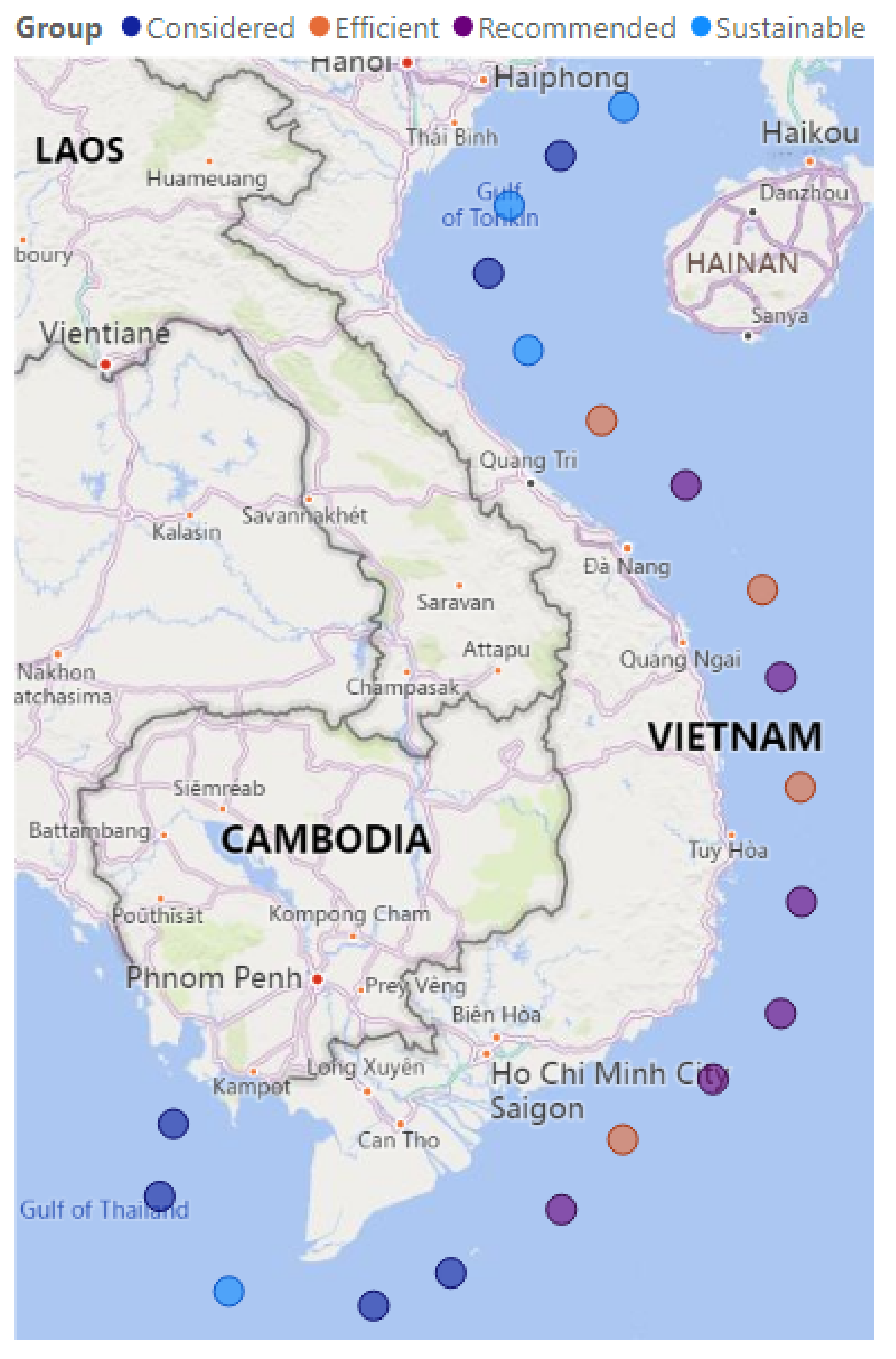
| Group | Locations |
|---|---|
| Recommended locations | WWS-7, WWS-9, WWS-11, WWS-12, WWS-13, WWS-15 |
| Sustainable locations | WWS-1, WWS-3, WWS-5, WWS-18 |
| Efficient locations | WWS-6, WWS-8, WWS-10, WWS-14 |
| Considered locations | WWS-2, WWS-4, WWS-16, WWS-17, WWS-19 |
Publisher’s Note: MDPI stays neutral with regard to jurisdictional claims in published maps and institutional affiliations. |
© 2022 by the authors. Licensee MDPI, Basel, Switzerland. This article is an open access article distributed under the terms and conditions of the Creative Commons Attribution (CC BY) license (https://creativecommons.org/licenses/by/4.0/).
Share and Cite
Le, M.-T.; Nhieu, N.-L. An Offshore Wind–Wave Energy Station Location Analysis by a Novel Behavioral Dual-Side Spherical Fuzzy Approach: The Case Study of Vietnam. Appl. Sci. 2022, 12, 5201. https://0-doi-org.brum.beds.ac.uk/10.3390/app12105201
Le M-T, Nhieu N-L. An Offshore Wind–Wave Energy Station Location Analysis by a Novel Behavioral Dual-Side Spherical Fuzzy Approach: The Case Study of Vietnam. Applied Sciences. 2022; 12(10):5201. https://0-doi-org.brum.beds.ac.uk/10.3390/app12105201
Chicago/Turabian StyleLe, Minh-Tai, and Nhat-Luong Nhieu. 2022. "An Offshore Wind–Wave Energy Station Location Analysis by a Novel Behavioral Dual-Side Spherical Fuzzy Approach: The Case Study of Vietnam" Applied Sciences 12, no. 10: 5201. https://0-doi-org.brum.beds.ac.uk/10.3390/app12105201