The Impact of Ensemble Techniques on Software Maintenance Change Prediction: An Empirical Study

Abstract

Various prediction models have been proposed by researchers to predict the change-proneness of classes based on source code metrics. However, some of these models suffer from low prediction accuracy because datasets exhibit high dimensionality or imbalanced classes. Recent studies suggest that using ensembles to integrate several models, select features, or perform sampling has the potential to resolve issues in the datasets and improve the prediction accuracy. This study aims to empirically evaluate the effectiveness of the ensemble models, feature selection, and sampling techniques on predicting change-proneness using different metrics. We conduct an empirical study to compare the performance of four machine learning models (naive Bayes, support vector machines, k-nearest neighbors, and random forests) on seven datasets for predicting change-proneness. We use two types of feature selection (relief and Pearson’s correlation coefficient) and three types of ensemble sampling techniques, which integrate different types of sampling techniques (SMOTE, spread sub-sample, and randomize). The results of this study reveal that the ensemble feature selection and sampling techniques yield improved prediction accuracy over most of the investigated models, and using sampling techniques increased the prediction accuracy of all models. Random forests provide a significant improvement over other prediction models and obtained the highest value of the average of the area under curve in all scenarios. The proposed ensemble feature selection and sampling techniques, along with the ensemble model (random forests), were found beneficial in improving the prediction accuracy of change-proneness.

1. Introduction

Numerous changes are applied to software systems during their development and maintenance, and predicting those classes that have a higher chance of being subjected to change in the future is a fundamental step in controlling and managing software development and in the creation of successful software products. Additionally, an early prediction of those changes assists software project managers and practitioners to manage resources and support decision-making [1]. Consequently, numerous prediction models have been created to predict change-proneness based on various source code metrics.

Change-proneness is an essential external quality attribute that can impact on the costs of maintenance and the quality of source code [2]. This paper considers change-proneness as a dependent variable to reflect that a change that has been performed in a given class (e.g., a line of code has been inserted, removed, or edited). Change-proneness is a Boolean variable that has the value TRUE if a change was made on the class (regardless of the type or number of changes) or FALSE if no change was made [3]. A number of studies have been conducted for predicting change-proneness using machine learning models which make use of source code metrics as dependent variables [4,5], but investigations are relatively rare compared with other software maintainability measurements [3].

Ensemble models, which combine several models instead of using just an individual model, have been applied in machine learning to improve performance. These models have an ability to decrease variance and have been proven to be of great practical value in various areas of software engineering [4,5,6]. However, there are few studies of prediction change-proneness using ensemble models [3].

Feature selection (FS) techniques have been introduced to address the problem of high-dimensional datasets, where the number of features is more than the number of observations. These techniques have the potential to increase prediction accuracy, reduce the time of model building, and identify the most vital features that affect the target attribute. Many studies have investigated various types of FS in software quality prediction and conclude that the ensemble FS techniques, which integrate the output of several FS strategies, are able to improve prediction accuracy [7], but, again, there is limited application of ensemble FS techniques in studies of software quality prediction [7].

Class imbalance is another dataset problem, where one class of the dataset has a small number of instances compared to the others, and machine learning models which fail to account for this end up predicting only from the majority class and ignoring the minority class. Several sampling techniques may be used to resolve this problem by adjusting the class distribution. These techniques are generally classified into three types: oversampling to increase the observations of the minority class (e.g., SMOTE [8] and UPSAMPLE [9]); undersampling to decrease the observations of the majority class (e.g., spread sub-sample [10] and random undersampling [11]), and ensemble sampling to combine the results of over- and undersampling (e.g., SMOTE and bootstrap sampling [12]). Although ensemble sampling techniques have been proven to increase the prediction accuracy, their application in software quality prediction is also relatively rare [9].

This study aims to investigate the performance of ensemble models, FS, and sampling techniques on the problem of predicting change-proneness using source code metrics. In order to achieve this aim, we examine four different scenarios on change-proneness datasets as follows: (a) datasets without FS and sampling techniques, (b) datasets with FS and without sampling, (c) datasets without FS and with sampling, and (d) datasets with FS and sampling. For this purpose, two types of filter-based feature-ranking techniques, namely, relief and Pearson’s correlation coefficient, were combined using the ensemble concept to determine the best metrics and tackle the problem of high dimensionality. The sampling techniques (i.e., SMOTE, spread sub-sample, and randomize) were also combined together in an ensemble to address the imbalance class problem.

Finally, three individual models (naive Bayes (NB), support vector machine (SVM), k-nearest neighbors (KNN)) and one ensemble model (random forest (RF)) were employed to predict change-proneness. These models were applied on seven publicly available datasets (i.e., antlr4, junit, MapDB, mcMMO, mct, oryx, and titan) extracted from open-source software systems [13]. The performance of the predicted models was compared and evaluated using the area under curve (AUC). The four research questions (RQs) were focused to accomplish the objectives of this paper:

• RQ1. What is the impact of ensemble FS techniques on the performance of prediction models?
• RQ2. What is the impact of ensemble sampling techniques on the performance of prediction models?
• RQ3. What is the impact of applying both ensemble FS and sampling techniques on the performance of prediction models?
• RQ4. What is the performance of the individual model and does the ensemble model (RF) outperform individual models?
• RQ5. What is the impact of the MTRY parameter tuning on RF?

The key contributions of this study are the following:

• The capability of the ensemble models, FS, and sampling techniques on predicting of change-proneness was evaluated using four different scenarios. To the best of the authors’ knowledge, this is the first study to investigate aspects such as the ensemble model, ensemble FS, and ensemble sampling techniques in predicting change-proneness. The most important finding was that RF provided a significant improvement over other prediction models and obtained the highest value of AUC in all scenarios.
• More informative and recommended measure was used for skewed datasets (i.e., AUC) to evaluate prediction accuracy (rather than using only measures based on accuracy such as precision or recall), and statistical test and effect size were performed on the results to evaluate the performance of the model.
• To make our predictive models refutable, conformable, and repeatable, the study used recent public datasets published in [13] and available on the PROMISE repository [14]. Two of these datasets are large and contain more than 1000 classes (i.e., mct and titan). Furthermore, a comprehensive replication package was provided which includes the new version of the datasets adapted for this study.
• The impact of MTRY parameter tuning in RF was explored using grid search.

The rest of the paper is organized as follows: Section 2 reviews the related work, Section 3 describes the research methodology, Section 4 presents the experimental design and setup, Section 5 discusses and analyzes the obtained results, Section 6 reports threats that could impact on the validity of this study, and Section 7 concludes this study with some directions for future work.

2. Related Work

The related work falls into four areas: studies that used change-proneness metrics, the role of ensemble prediction models in various area of software engineering problems, the use of feature selection to resolve the issue of high dimensionality, and sampling strategies to address the problem of imbalanced classes.

2.1. Change-Proneness Metrics

Metrics are measures of software engineering attributes, and several research studies have explored the use of source code metrics as independent variables when predicting change-proneness [3]. Most of the studies [5,15] have only used the Chidamber and Kemerer (C&K) metrics: weighted methods per class (WMC), depth of inheritance tree (DIT), number of children (NOC), coupling between object classes (CBO), response for a class (RFC), and lack of cohesion in methods (LCOM) [16]. These studies reveal that the C&K metrics are good predictors of change-proneness [5,15]. Catolino and Ferrucci investigated various metrics (product, process, and developer-related factors) to predict change-proneness and observed that the models created using developer-related factors outperformed the other models that were built using product and process metrics [4]. Malhotra and Khanna explored the effectiveness of a set of source code metrics in predicting change-proneness based on different features of the software, such as size, coupling, cohesion, and inheritance [17]. In addition to this study, they examined the relationship between object-oriented metrics and change proneness and found that this relationship occurred and machine learning models performed better than the statistical methods [18]. Kumar et al. used ten source code metrics and performed FS techniques to determine the best metrics with an objective to increase the prediction accuracy of predicting change-proneness. They found that these metrics are able to predict change-proneness accurately [19]. Lu et al. employed 62 different object-oriented metrics, involving 20 coupling metrics, 7 size metrics, 17 inheritance metrics, and 18 cohesion metrics on 102 Java systems to predict change-proneness [20]. The results obtained from this study indicate that size metrics achieved high prediction accuracy, whereas coupling and cohesion metrics produced low prediction accuracy, and inheritance metrics attained poor performance to predict change-proneness [20]. From these various studies, a clear association between object-oriented metrics and change-proneness emerges and it is safe to conclude that these metrics can be used as predictors for change-proneness.

2.2. Ensemble Prediction Models

One of the main benefits of the ensemble models is to reduce the prediction variance that is a common factor in machine learning models [21]. Several studies have explored the application of ensemble models in fault or defect prediction problems and recorded high accuracy from using approaches such as random forest [4,22], bagging and boosting [23], and adaptive selection of classifiers in bug prediction [6]. Previous studies have also stated the success of using ensemble models to predict effort estimation using techniques such as bagging [24]; ensembles of linear methods [25]. Ensemble models have also been used to predict change-proneness, such as hard instance ensemble classifier [5], random forest [4], and majority voting [19]. Among several ensemble models implemented in studies of the software engineering field, a number of these studies emphasized that RF outperforms other prediction models and produces a high improvement in the prediction accuracy [4,22]. These findings motivate us to use ensemble models (and RF in particular) in this study. Although several studies have used RF with default parameter settings [4,22], there is no theoretical justification to apply these default values [26]. As the performance of RF depends on parameter values, it is necessary to investigate RF tuning based on the parameters [26]. Therefore, the impact of MTRY parameter tuning in RF using the grid search was investigated in this study.

2.3. Ensemble Feature Selection Techniques

The major purpose of FS is to identify the best subset of attributes (i.e., independent variables) to predict the target attribute (i.e., dependent variable). A range of various FS techniques have been used in the domain of software engineering prediction (e.g., defect, change metric, maintainability index, and change-proneness) [7]. Previous work by the authors also used FS techniques to achieve better prediction accuracy [7]. Moreover, using ensemble FS techniques, which combines the output of several FS techniques, outperformed individual FS techniques in three studies [7].

2.4. Ensemble Sampling Techniques

Imbalanced classes occur when the quantity of one class in the dataset is far less than that of another. This problem can cause machine learning models to bias their predictions towards majority classes and ignore minority classes, resulting in a high prediction accuracy on the majority class at the expense of the minority class. To resolve this issue, sampling techniques can be used and have been applied successfully in various fields. Within the software engineering domain, synthetic minority oversampling technique (SMOTE) has been used in refactoring prediction [8]. Sampling techniques can divided into three types: oversampling to increase the observations of the minority class (e.g., SMOTE [8] and UPSAMPLE [9]); undersampling to decrease the observations of the majority class (e.g., spread sub-sample [10] and random undersampling [11]), and ensemble sampling to combine the results of over- and undersampling (e.g., SMOTE and bootstrap sampling [12]). These ensemble sampling techniques were found to be particularly effective in improving the performance of prediction models [9]. Table 1 summarizes the related work.

To fill the gaps in these previous studies, the empirical study was designed to predict change-proneness using three individual models and one ensemble model. Additionally, ensemble FS techniques were used, including relief and Pearson’s correlation, which are the most popular FS techniques used in [7]. To make the predictive models refutable, confirmable, and repeatable, recent public datasets published in [13] and available on the PROMISE Repository [14] were used.

Table 1. Summary of the related work.

The Area of Related Work	Ref.	Advantages	Disadvantages	Contributions of This Study
Change-proneness metrics	[5,15]	A limited number of metrics have been used by previous studies as predictors of change-proneness.	Several metrics have not been investigated by previous studies.	This study explores a total of 102 metrics.
Ensemble prediction models	[4,22]	Ensemble models have yielded improved prediction accuracy over individual models.	Limited previous studies used ensemble models to predict change-proneness,	This study investigates the performance of RF and the impact of the influence of Mtry parameter tuning using the grid search.
Ensemble feature selection techniques	[7]	Using ensemble FS techniques outperformed individual FS techniques.	No previous studies used ensemble FS to predict change-proneness.	This study performs ensemble FS (i.e., relief and Pearson’s correlation coefficient).
Ensemble sampling techniques	[8,9]	Using ensemble sampling techniques performed better than individual sampling techniques.	No previous studies used ensemble sampling to predict change-proneness.	This study applies ensemble sampling (i.e., SMOTE, spread sub-sample and randomize).

Table 1. Summary of the related work.

The Area of Related Work	Ref.	Advantages	Disadvantages	Contributions of This Study
Change-proneness metrics	[5,15]	A limited number of metrics have been used by previous studies as predictors of change-proneness.	Several metrics have not been investigated by previous studies.	This study explores a total of 102 metrics.
Ensemble prediction models	[4,22]	Ensemble models have yielded improved prediction accuracy over individual models.	Limited previous studies used ensemble models to predict change-proneness,	This study investigates the performance of RF and the impact of the influence of Mtry parameter tuning using the grid search.
Ensemble feature selection techniques	[7]	Using ensemble FS techniques outperformed individual FS techniques.	No previous studies used ensemble FS to predict change-proneness.	This study performs ensemble FS (i.e., relief and Pearson’s correlation coefficient).
Ensemble sampling techniques	[8,9]	Using ensemble sampling techniques performed better than individual sampling techniques.	No previous studies used ensemble sampling to predict change-proneness.	This study applies ensemble sampling (i.e., SMOTE, spread sub-sample and randomize).

3. Research Methodology

The main aim of this study is to evaluate the impact of ensemble models (RF), ensemble FS (relief and Pearson’s correlation coefficient), and ensemble sampling techniques (SMOTE, spread sub-sample, and randomize) on the performance of change-proneness prediction models. The interaction between feature selection and sampling is examined via the following four scenarios:

• First scenario: datasets without FS and sampling techniques.
• Second scenario: datasets with FS and without sampling techniques.
• Third scenario: datasets without FS and with sampling techniques.
• Fourth scenario: datasets with FS and sampling techniques.

Table 2. Scenarios in the empirical study.

	Feature Selection Techniques	Sampling Techniques
First scenario	NO	NO
Second scenario	YES	NO
Third scenario	NO	YES
Fourth scenario	YES	YES

illustrates the scenarios explored in the empirical study. These scenarios were studied because the datasets present two problems: (I) high dimensionality and (II) imbalanced classes. This poses a difficulty regarding which model to apply first: the FS for the high dimensionality or sampling techniques for the imbalanced classes. Consequently, these scenarios help to evaluate and compare the impact of ensemble FS and sampling techniques separately in the second and third scenarios, and together in the fourth scenarios. The sampling and FS techniques are discussed later in Section 4.1.4: Data Preprocessing.

3.1. Framework of the Research Method

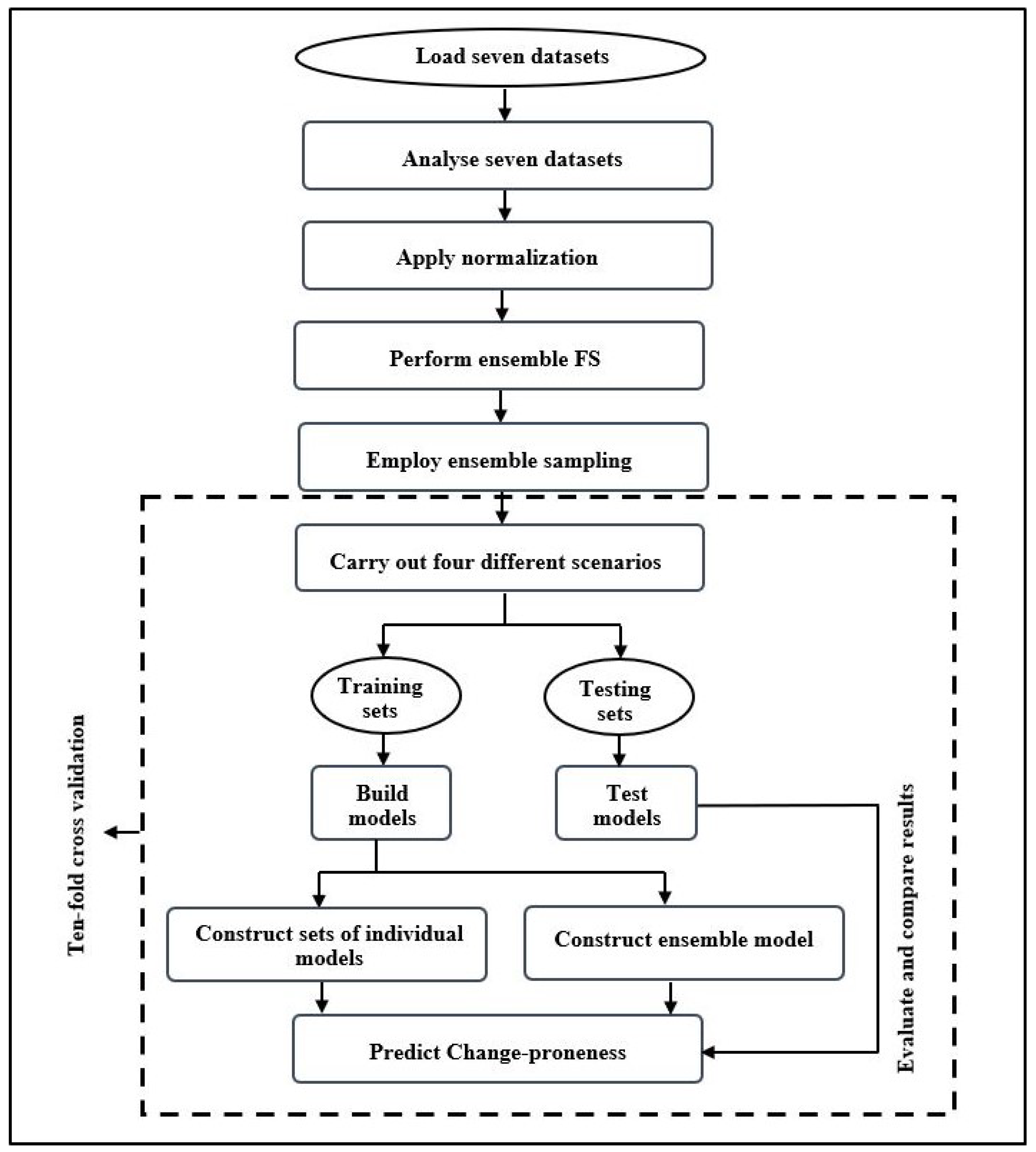
Figure 1 shows the framework of the research method, which contains several steps:

• Step 1. We load the datasets, details of which, along with independent and dependent variables are described in Section 4.1.
• Step 2. We analyze the datasets to eliminate any metrics which contain empty values, and redundant metrics that are strongly correlated with each other. This step is performed using descriptive statistics and Spearman correlation.
• Step 3. We apply normalization to the bring the values of the dataset into the range 0 to 1.

  Figure 1. Framework of the research method.

  Figure 1. Framework of the research method.
• Step 4. We perform ensemble FS using the relief and Pearson’s correlation coefficients to select the best ten metrics (independent variables) from each dataset.
• Step 5. We employ ensemble sampling techniques, namely, SMOTE, to perform oversampling by increasing the number of the minority class, and spread sub-sample to perform undersampling by decreasing the number of the majority class, and randomization to rearrange the instances randomly. The main reason for applying this randomization is to avoid overfitting in ten-fold cross-validation because SMOTE inserts the additional instances at the end of the dataset.
• Step 6. We conduct four different scenarios across seven change-proneness datasets (see Table 1) as follows: First scenario (i.e., Step 1, Step 2, and Step 3), Second scenario (i.e., Step 1, Step 2, Step 3, and Step 4), Third scenario (i.e., from Step 1, Step 2, Step 3, and Step 5 without Step 4) and Fourth scenario (i.e., Step 1, Step 2, Step 3, Step 4, and Step 5) (see Figure 2).
• Step 7. We divide the datasets into training and test sets using ten-fold cross-validation.
• Step 8. We construct the prediction models, which encompass three individual models (NB, SVM, and KNN) and one ensemble model (RF).
• Step 9. We predict change-proneness and evaluate and compare the results of the four prediction models across the four scenarios to determine the most accurate prediction model using AUC as the measure of comparison.

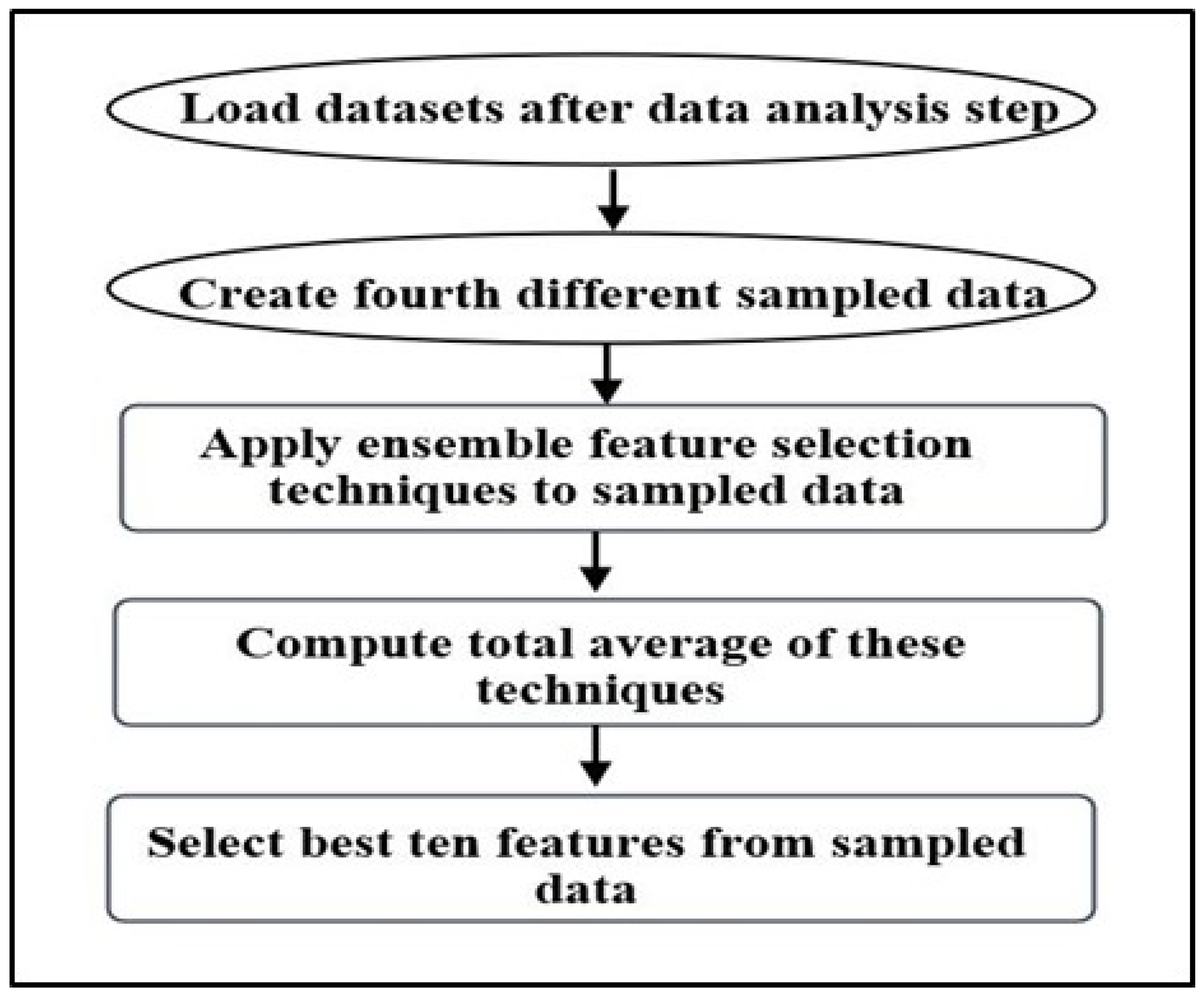
3.2. Framework of the Fourth Scenario

The fourth scenario is designed to resolve both problems (high dimensionality and imbalanced class) and to avoid biased results from the sampling techniques in the fourth scenario. Therefore, the ensemble FS techniques were applied using different sampled data purely for the purpose of providing effective FS techniques. Figure 2 illustrates the framework for the fourth scenario that include five primary steps.

• Step 1. We load seven datasets after the data analysis step (Step 2 in previous section).
• Step 2. We create a fourth set of differently sampled data purely for the purpose of performing FS techniques:

  1.

  Datasets without sampling.

  2.

  Datasets with SMOTE sampling.

  3.

  Datasets with SMOTE and spread sub-sample with the parameter set to 1, where these parameters define the distribution spread ratio between the majority and minority classes as 50:50.

  4.

  Datasets with SMOTE and spread sub-sample with the parameter set to 2.1, where these parameters define the distribution spread ratio between the majority and minority classes as 35:65.

• Step 3. We apply ensemble FS using two filter-based feature ranking techniques, namely relief and Pearson’s correlation coefficient on all sampled data in Step 2.
• Step 4. We compute the average of the feature ranking techniques in Step 3 across all sampled data in Step 2.
• Step 5. We select the best ten features that have the highest ranking from the sampled datasets in the third scenario. Therefore, the main difference between the third and fourth scenario is performing ensemble FS techniques in the fourth scenario. However, both the third and fourth scenarios used the same ensemble sampling techniques, namely, SMOTE, spread sub-sample with 2.1 ratio, and randomize.

4. Experimental Design and Setup

The following subsections present a description of the datasets used in this empirical study, along with the explanation of the dependent and independent variables. They also provide details about the dataset analysis using descriptive statistics and Spearman correlation. Finally, they explain the data preprocessing that includes normalization, FS, and sampling.

4.1. Datasets

In this empirical study, we used seven publicly available datasets containing details of source code metrics and refactoring collected from a total of 37 subsequent releases of systems from seven open-source Java systems located in GitHub [27]. These are combined into one manually validated dataset for each of the seven systems [13]. We select these datasets particularly because many research studies have explored the utilization of prediction models in software maintainability. Most of these studies have predicted change maintenance effort using CHANGE metric and maintainability index, but little progress has been made in predicting change-proneness in software maintainability [1]. In addition, these datasets are the only datasets available on the PROMISE repository and suitable for predicting change-proneness. To the best of the author’s knowledge, these datasets are considered the newest datasets in software maintainability prediction and have not been utilized in previous studies to predict change-proneness.

Table 3. Summary of the datasets.

Dataset Name	# Classes	# Release	Time Interval	URL
antlr4	436	5	21 January 2013–22 January 2015	https://github.com/antlr/antlr4 (accessed on 4 June 2020)
junit	657	8	13 April 2012–28 December 2014	https://github.com/junit-team/junit (accessed on 4 June 2020)
MapDB	439	6	1 April 2013–20 June 2015	https://github.com/jankotek/MapDB (accessed on 4 June 2020)
mcMMO	301	5	24 June 2012–29 March 2014	https://github.com/mcMMO-Dev/mcMMO (accessed on 4 June 2020)
mct	2162	3	30 June 2012–27 September 2013	https://github.com/nasa/mct (accessed on 4 June 2020)
oryx	536	4	11 November 2013–10 June 2015	https://github.com/cloudera/oryx (accessed on 4 June 2020)
titan	1486	6	7 September 2012–13 February 2015	https://github.com/thinkaurelius/titan (accessed on 4 June 2020)

provides a summary of the datasets used in this study, which includes the dataset name, number of classes, number of releases, time interval, and URL [13].

The datasets were initially collected to investigate the impact of code refactoring (changes made to the structure of the internal source code which do not affect the functionality or external behavior of the code [8]) on maintainability, and the original datasets contain source code metrics including refactoring metrics, along with a score for maintainability at both method and class levels [13] We removed some metrics to convert the refactoring datasets into ones that are suitable to predict change-proneness at the class level. To achieve this, we performed three steps:

• Step 1. We removed the relative maintainability index (RMI), which is the dependent variable in the original datasets, because it is a derived variable (from some of the independent variables which will cause any machine learning model to just learn the function that defines it) and also not an accurate reflection of maintenance effort.
• Step 2. We convert the total number of refactoring changes in each class (Refact_Sum) to a binary variable (Change_Prone) that indicates whether a change has taken place in each class during the maintenance period. Refact_Sum contains the total number of source code refactoring operations that have been applied in each class in a certain observation period. The reason for this is that the number of refactoring is very low, ranging from 0 to 8 with a median of zero in all datasets (see Table 4). Change_Prone is set to TRUE if any refactoring changes were made on the class (regardless of the number) or FALSE if no refactoring changes were made.

  Table 4. Descriptive statistics of Refact_Sum.

  	MIN	MAX	Standard Deviation	Average	Median
  antlr4	0	8	0.70	0.13	0
  junit	0	3	0.21	0.02	0
  MapDB	0	2	0.13	0.01	0
  mcMMO	0	2	0.18	0.02	0
  mct	0	5	0.18	0.01	0
  oryx	0	6	0.35	0.05	0
  titan	0	3	0.13	0.01	0

  Table 4. Descriptive statistics of Refact_Sum.

  	MIN	MAX	Standard Deviation	Average	Median
  antlr4	0	8	0.70	0.13	0
  junit	0	3	0.21	0.02	0
  MapDB	0	2	0.13	0.01	0
  mcMMO	0	2	0.18	0.02	0
  mct	0	5	0.18	0.01	0
  oryx	0	6	0.35	0.05	0
  titan	0	3	0.13	0.01	0

• Step 3. We remove 23 refactoring metrics from the independent variables in the refactoring datasets. These are related to specific refactoring changes that have taken place and are not relevant for the prediction of change proneness and would also prejudice the outcome of the study as they identify when a change has been made.

After applying these steps, we are left with (Supplementary C in the reproduction package) a new version of the refactoring datasets, referred to as the change-proneness datasets, which contain 102 metrics as independent variables and Change_Prone metric as dependent variable. The explanation of independent and dependent variables will be presented in the next two sections.

4.1.1. Dependent Variable: Change-Prone

As already mentioned, Change_Prone is used in this study as dependent variable to reflect that a change (insertion, removal, or edit) has been performed on a given class for a version of the system.

Table 5. Number of true and false values in the change-proneness attribute.

Dataset Name	# Instances	# True Value	% True Value	# False Value	% False Value	Category of Difference between True and False
antlr4	436	23	5.28%	413	94.72%	Small
junit	657	9	1.37%	648	98.63%	Medium
MapDB	439	4	0.91%	435	99.09%	Large
mcMMO	301	4	1.33%	297	98.67%	Medium
mct	2162	15	0.69%	2147	99.31%	Large
oryx	536	15	2.80%	521	97.20%	Small
titan	1486	13	0.87%	1473	99.13%	Large

summarizes the number of true and false values for the variable, which demonstrates the imbalance between the two values. We categorized this difference between values into small, medium, and large according to the percentage of true values in our datasets, where values less than 1% correspond to a large difference, values less than 2% are a medium difference, and values out of these ranges are a small difference. However, it should be pointed out that all the percentages of true values in Table 4 are very small, ranging from 0.69% to 5.28%.

4.1.2. Independent Variables: Source Code Metrics

The independent variables include 125 metrics, which can be grouped into ten categories as follows: cohesion, complexity, coupling, documentation, inheritance, size, code duplication, warning, rules, and refactoring.

Table 6. Metrics used as independent variables and their category.

Category	Metrics
Cohesion	LCOM5
Complexity	NL, NLE and WMC
Coupling	CBO, CBOI, NII, NOI and RFC
Documentation	AD, CD, CLOC, DLOC, PDA, PUA, TCD, and TCLOC
Inheritance	DIT, NOA, NOC, NOD and NOP
Size	LOC, LLOC, NA, NG, NLA, NLG, NLM, NLPA, NLPM, NLS, NM, NPA, NPM, NS, NOS, TLOC, TLLOC, TNA, TNG, TNLA, TNLG, TNLM, TNLPA, TNLPM, TNLS, TNM, TNPA, TNPM, TNS and TNOS
Code duplication	CCL, CCO, CC, CI, CLC, CLLC, LDC and LLDC
Warning	WarningBlocker, WarningCritical, WarningInfo, WarningMajor and WarningMinor
Rules	Android Rules, Basic Rules, Brace Rules, Clone Implementation Rules, Clone Metric Rules, Code Size Rules, Cohesion Metric Rules, Comment Rules, Complexity Metric Rules, Controversial Rules, Coupling Metric Rules, Coupling Rules, Design Rules, Documentation Metric Rules, Empty Code Rules, Finalizer Rules, Import Statement Rules, Inheritance Metric Rules, J2EE Rules, JUnit Rules, Jakarta Commons Logging Rules, Java Logging Rules, JavaBean Rules, MigratingToJUnit4 Rules, Migration Rules, Migration13 Rules, Migration14 Rules, Migration15 Rules, Naming Rules, Optimization Rules, Security Code Guideline Rules, Size Metric Rules, Strict Exception Rules, String and StringBuffer Rules, Type Resolution Rules, Unnecessary and Unused Code Rules and Vulnerability Rules’

lists metrics used as independent variables and their category (the refactoring metrics are excluded as they were removed in the data preprocessing step so we are left with 102 metrics), where the description of the abbreviation of these metrics is provided in Supplementary C in the reproduction package). All the independent variables are numeric and they were collected using the SourceMeter static code analysis tool [28]. Hegedűs et al. describe how they extracted these metrics [13], and they are also defined on the tool’s website [28].

4.1.3. Dataset Analysis

The primary objective of the dataset analysis is to detect any attributes that contain values that might cause problems when building any prediction models and produce skewed or misleading results. The descriptive statics of these metrics are presented in Supplementary A in the reproduction package. The minimum values are zero or one in all datasets. In contrast, the maximum values are 575 in CLOC metric in antlr4 dataset, 662 in TNM metric in junit dataset, 11,272 in LLOC metric in MapDB dataset, 1160 in LOC metric in mcMMO dataset, 1390 in WarningInfo metric in mct dataset, 179 in NII metric in oryx dataset, and 1104 in WarningMinor metric in titan dataset. Thus, there was a considerable difference between the minimum and maximum values in all datasets. For this reason, normalization was applied, which will be described in the next section. Another important finding was that the average values of WarningInfo metrics were high in all datasets, ranging from 8 to 15. The remaining metrics have different values of descriptive static, which suggests that the datasets have varying characteristics.

Firstly, we drop metrics that have zero values (Supplementary B in the reproduction package), and therefore cannot be used as predictors (see Briand et al. [29]). In total, 21 metrics were removed from some of the datasets, and 7 metrics were removed from all datasets (see summary metrics removed in the Supplementary A in the reproduction package).

Secondly, we calculate the Spearman correlation, which is a well-known statistical measurement to compute the strength (i.e., strong or weak) and the direction (i.e., positive or negative) of relationship between two ranked variables [30]. Spearman correlation was selected in this study because it is appropriate for the monotonic relationship, which indicates that if one variable increases, the other variable either increases or decreases. From this, we create a correlation matrix to identify the dependence between variables (Supplementary B in the reproduction package). This correlation was used to remove redundant variables and prevent multicollinearity that occurs when one independent variable in a prediction model can be predicted from other independent variables with a high accuracy [31]. We eliminate one of a pair of variables that have a high strong correlation. In Supplementary B, a green color in the correlation matrix refers to the high strong correlation, where the correlation coefficient is over than +0.9. Supplementary B also provides the results of the strong correlations and shows the attributes that were removed using Spearman correlation. This analysis results in between 31 and 38 metrics being removed from the datasets (the correlations were not completely consistent between the datasets, hence the different values—see

Table 7. Number of metrics removed in each data analysis technique.

Analysis Technique	Description of Metrics Removed	Datasets
		antl4	junit	MapDB	mcMMO	mct	oryx	titan
		Number of metrics removed
Descriptive statistics	Remove metrics with zero values	13	15	14	17	9	15	12
Spearman correlation	Remove metrics with a strong correlation with others	35	32	31	37	33	32	38
		Number of metrics remained
		54	55	57	48	60	55	52

), leaving between 48 and 60 attributes.

4.1.4. Data Preprocessing

Data preprocessing is an important data mining technique performed to resolve issues related to the datasets, such as incorrect, missing, imbalanced, and inconsistent data [32]. The datasets used in this chapter had several problems that required the application of some of the data preprocessing techniques. Initially, the values in the independent variables have a different range, so we apply normalization to bring them all into the range 0 to1. Additionally, there are the problems of high dimensionality and class imbalance mentioned earlier which require the application of feature selection and sampling techniques. These three techniques are described in the next sections.

Normalization

Normalization is a common technique employed when the values of numeric data have very different scales. It is also essential for the application of some machine learning models that use scale-sensitive distance metrics, such as KNN, which uses Euclidean distance to identify the nearest neighbors. In this study, the dataset is linearly rescaled using min-max normalization to normalize all numeric values in our datasets to the interval [0, 1] [32]. Equation (1) defines min–max normalization, where min and max are the minimum and maximum values in the datasets, respectively, and value is the value being normalized:

$$\mathrm{Min}-\mathrm{Max} \mathrm{Normalization} =\frac{\mathrm{value}-\min }{\max -\min }$$

(1)

Feature Selection

Having identified and addressed any multicollinearity problems, FS is performed in the second and fourth scenarios as an additional step to improve the quality of the dataset as it still contains numerous attributes.

In this study, we use the ensemble method to determine the best features using two types of filter-based feature ranking techniques, namely, relief and Pearson’s correlation coefficient. We chose these types because relief is the most frequently used in the selected primary studies proposed in [7] and the Pearson’s correlation coefficient is the second most popular. First, we apply these techniques on the datasets that assign a score to each feature; then we calculate the average of the two techniques and select the ten highest-scoring features (there is no clear evidence in the literature on a suitable number of features to select [11], so the number of features chosen was determined by previous studies either by identifying the number of features [33] or employing a cut-off value [34]). We apply these techniques using WEKA with the parameters set to the default values.

Sampling

In this study, all the datasets have a very small minority of true values (see Table 5) which can lead to the creation of biased prediction models. To resolve the class imbalance problem, sampling techniques are introduced, including oversampling to increase the observations of the minority class and undersampling to decrease the observations of the majority class. The main advantage of oversampling is to maintain all the observations of both the majority and minority classes, but this may lead to overfitting. In contrast, undersampling eliminates some observations and may remove essential observations. However, there was no clear indication of which technique performs better [35], and so ensemble sampling techniques are carried out in this study to resolve the imbalanced class problem and improve the overall performance. We apply sets of three sampling techniques that involve SMOTE for oversampling, spread sub-sample for undersampling, and randomize for mixing the order of the instances. Ensemble sampling integrates the results of over- and undersampling, where SMOTE inserts more true values, and spread sub-sample removes some false values.

4.2. Prediction Models

The choice of the individual models was based on their popularity and performance. Based on the authors’ systematic review [7], we selected the most frequently used individual and ensemble models that are suitable for the software quality classification problems. These include three individual models (i.e., NB, SVM, and KNN), and one ensemble model, RF. These models are considered among the best five models for classification problems [36], but also have their own strengths and weaknesses. The main advantage of NB is its ability to estimate the parameters and a model from a smaller proportion of the dataset, and then it produces means and variances of the variables for each class. Nevertheless, the disadvantage of NB is to assume all features independent from each other [37]. SVMs have efficient execution without dependence on the dimensionality of the input space and superior performance with excellent accuracy prediction [38,39]. KNN is simple to perform and easy to understand, but it does not work well if the datasets have outliers, noisy, or missing values neighbors [40]. RF is less sensitive to the parameter used, so it creates easily. RF are less sensitive to the parameter used, so are easy to create. In addition, RF can resolve the overfitting problem more efficiently and can perform tree pruning faster than individual decision trees [26]. The open-source Waikato Environment for Knowledge Analysis (Weka) tool is used to construct prediction models, and the default values of the models’ parameters were used [41]. More details of the models are outlined in the following sections.

4.2.1. ZeroR

ZeroR is a very simple classifier based on the dependent variable only (i.e., change-proneness) that disregards other independent variables and bases the prediction on the majority classes (i.e., the mode values) [42]. It is performed purely to identify a baseline that is used as a benchmark to evaluate the performance of the machine learning models (which, ideally, should be of higher accuracy than ZeroR) [43]. Equation (2) defines mode, where “L” “H1” is the size of the class interval, “Fm” is the frequency of the modal class, “F1” is the frequency of the class preceding the modal class, and “F2” is the frequency of the class succeeding the modal class [44]:

$$Mode = L + H \frac{(Fm - F1)}{\left(Fm - F1\right) + (Fm - F2)}$$

(2)

4.2.2. Naive Bayes

NB is a probabilistic algorithm that relies on Bayes theorem to predict the class for each row. NB applies independence assumptions, which consider features to be independent of each other. NB uses estimator classes, and this estimation is performed using the maximum likelihood method [45]. Equation (3) represents the Bayes theorem, where P(c|x) is the posterior probability of class, P(x) is the prior probability of predictor, P(c) is the prior probability of class, and P(x|c) is the likelihood which is the probability of predictor specific class [37].

$$P\left(c\left|\phantom{cx}\right. x\right)= \frac{P\left(x\left|\phantom{xc}\right. c\right)P\left(c\right)}{P\left(x\right)}$$

(3)

4.2.3. K-Nearest Neighbors

KNN, which is called instance-based learning (IBK), is classified as a lazy learner. First, KNN is calculated by selecting the closest neighbors in the training data to generate the target data with regard to the feature space. This selection is employed using the Euclidean (or other specified) distance measure. After that, majority voting, or another decision rule, can be performed to categorize the new instances [40].

4.2.4. Support Vector Machine

SVM is considered a category of generalized linear classifiers that convert the original dataset training to a higher dimension using a nonlinear mapping [32]. Then, it creates the linear optimal separating hyperplane to separate the dataset into two classes. Furthermore, there are two lines that create a maximal margin hyperplane, which makes the boundary line, where the instances lie on the margins of the maximum margin hyperplane. We used sequential minimal optimization (SMO) in Weka as the implementation for SVM, and this has several features, such as the ability to handle very large datasets and faster model creation for sparse datasets and linear SVM [46]. Additionally, it has the ability to handle complex nonlinear decision boundaries and is less prone to overfitting than other models. These features help SVM to reduce prediction error and improve overall prediction accuracy [32].

4.2.5. Random Forest

Random forest is an ensemble model that build a forest of numerous unpruned decision trees from the training dataset. Then, it uses the mode of the classes of the individual trees on the testing dataset to make a prediction. RF integrates tree predictors that depend on the values of a random vector sampled individually, along with the same distribution for the whole trees in the forest. Applying this random selection of features leads to higher error rates than those in AdaBoost [47], but the random forest is better in terms of dealing with noisy data [48]. Moreover, this algorithm performs bagging on features based on majority voting and selects the dependent variables which have the highest votes [48]. In this study, random forest integrates algorithms of the same types (i.e., decision trees), so it can be classified as a homogeneous ensemble model. RF depends on four parameters: the number of trees to grow, the sub-sample size common to each tree, the tree depth, and the number of variables randomly sampled for splitting [26]. We used the default parameters in Weka, where Weka creates a forest of several decision trees as the base models and initializes this forest to 100 tree instances [49].

4.3. Prediction Accuracy Measures

The following subsections provide the explanation of the performance measures used in this empirical study, along with the description of the statistical tests and effect size.

4.3.1. Performance Measures

Several measures have been proposed in the literature to evaluate the accuracy of the prediction models in software engineering problems [50]. In this study, only one prediction accuracy measure, which is AUC, is used to evaluate and compare the performance of prediction models. AUC is based on the ROC (receiver operating characteristic) that graphs the true positive rate (TPR) on the y-axis against the false positive rate (FPR) on the x-axis at different threshold settings [51]. AUC ranges from 0 to 1, where the greater value indicates better results and 1 is the optimal result (a perfect classifier). Additionally, 0.5 indicates no discrimination, a value from 0.7 to 0.8 indicates an acceptable result, a value from 0.8 to 0.9 is recognized as excellent, and any values greater than 0.9 are considered outstanding results [52].

According to a study published in [7], AUC was the principle and most frequently evaluation measure used for classification problems in software quality prediction. In addition, it is considered well-known and commonly employed in software maintainability prediction along with change-proneness prediction [13].

Equation (4) calculates the value of $AUC$, where i represents observations, $\left(1-\beta \right)$ represents the TPR = $\frac{TP}{TP + FN}$, $\alpha$ represents the FPR =$\frac{FP}{FP + TN}$, and these values are extracted from the confusion matrix presented in Table 8.

$$AUC= \sum _i\left\{\left( 1-{\beta }_i . \Delta \alpha \right)+\frac{1}{2}[\Delta \left(1-\beta \right).\Delta \alpha ]\right\}$$

(4)

$\Delta \left(1-\beta \right)$ indicates $\left( 1-{\beta }_i \right)- \left( 1-{\beta }_{i-1} \right)$, and $\Delta \alpha$ indicates ${\alpha }_{i }-{\alpha }_{i-1}$

Table 8. Confusion matrix.

	Predicted Class (No)	Predicted Class (Yes)
Actual class (No)	True negatives (TN)	False positive (FP)
Actual class (Yes)	False negative (FN)	True positive (TP)

Table 8. Confusion matrix.

	Predicted Class (No)	Predicted Class (Yes)
Actual class (No)	True negatives (TN)	False positive (FP)
Actual class (Yes)	False negative (FN)	True positive (TP)

4.3.2. Statistical Tests and Effect Size

Test of significance is used in this study to validate the results according to a defined hypothesis. We carried out a one-way analysis of variance (ANOVA) F test [53] on the performance of AUC. We selected ANOVA because there are more than one pair (i.e., four prediction models). Therefore, this test is performed to investigate if there exists a significant difference between the group population means (i.e., performance of the prediction models). Statistical significance is defined in this study as ($\alpha$ = 0.05) and we evaluate and compare the p-value with this defined value. If the p-value is smaller than $\alpha$ then the H${}_0$ (the null hypothesis, that there is not a statistically significant difference between all the group population means) is rejected.

In addition, to further understand the strength of a result, the effect size is used in this study too, which is considered an essential component to complement significance tests [54]. From the various effect size measures introduced in the literature, eta-squared ($\eta$${}^2$) is selected in this study because this is a suitable measure for ANOVA [54]. Cohen proposed the standard classifications of the effect sizes, which are small (≈0.01), medium (≈0.06), and large (≈0.14) [55]. Equation ((5)) computes the value of $\eta$${}^2$.

$${\eta }^2=\frac{SS \mathrm{effect}}{SS \mathrm{total}}$$

(5)

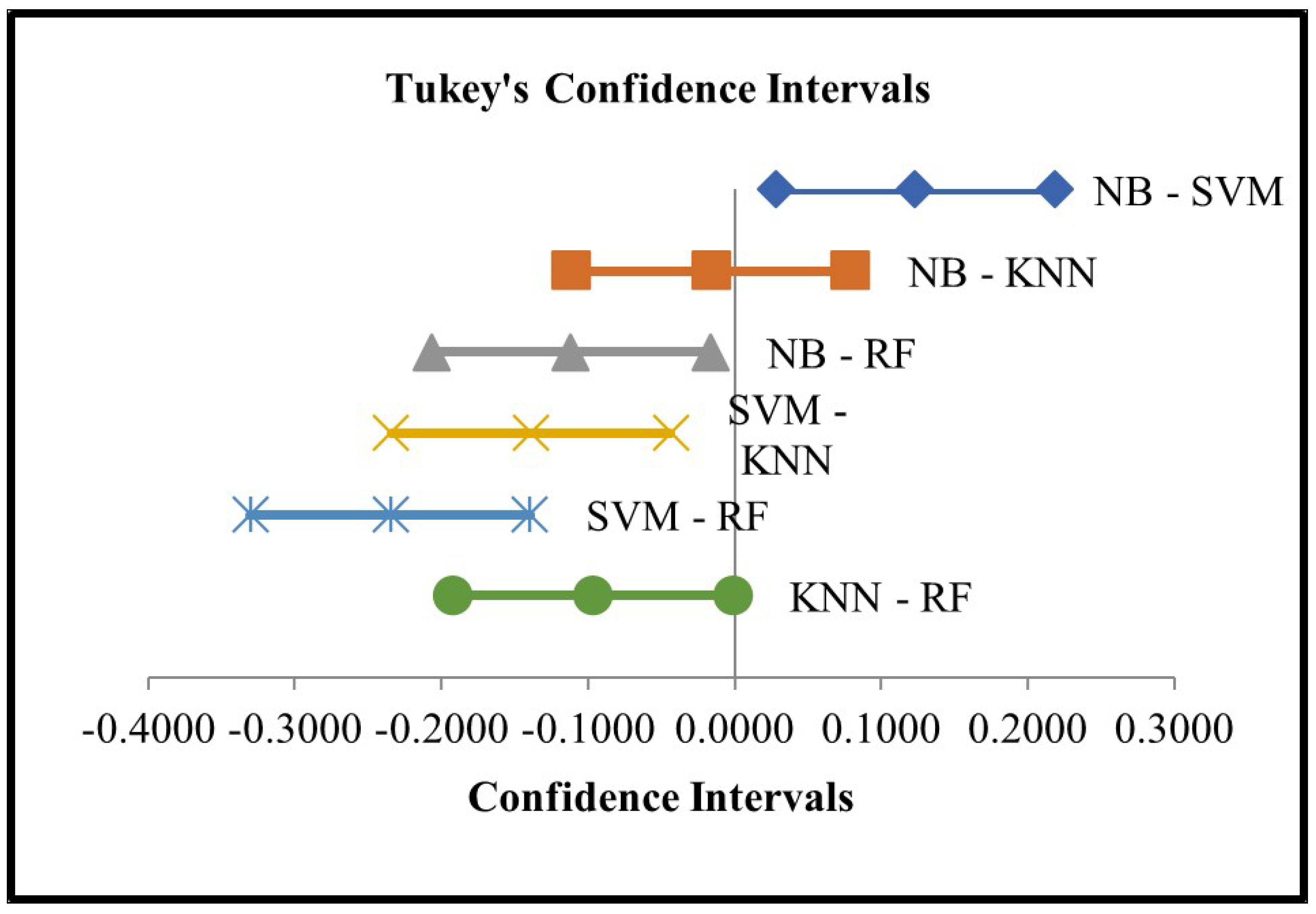
SSeffect is the sum of squares of the effect, and SStotal is the total sum of squares [54]. Additionally, If H${}_0$ is rejected, we apply multiple comparisons using a plot chart of Tukey’s confidence intervals [53] to identify which pairs are significantly different. If a confidence interval does not include 0 then the pair is significantly different.

4.3.3. Grid Search

Parameter tuning is performed on RF using a grid search with ten-fold cross-validation. Grid search is the process of exploring the search space of the hyperparameter values with the specification of parameter pairs and evaluation measurement (e.g., AUC). This process is iterated via ten-fold cross-validation until the optimal hyperparameters are determined, which results in the highest prediction accuracy [56]. Grid search is created using the tunegrid function in R, along with the randomForest, mlbench, and caret packages to build the RF model. RF depends on four parameters: the number of trees to construct, the sub-sample size common to each tree, the tree depth, and the number of variables randomly sampled for splitting [26]. However, only the last parameter was tuned (i.e., the number of variables randomly sampled for splitting), using Mtry variable in R. The rationale for focusing on just the Mtry parameter is because there is no clear indication or theory of which value of this parameter is more appropriate under most circumstances [26]. Therefore, the grid search used in Section 5.3.7 is considered a linear search, in which the vector of candidate values ranges from 1 to 15. These values were initialized because there is no recommendation to select the number Mtry parameter [26].

5. Results and Analyses

This section provides the answers to the RQs and discusses the results obtained. First, we present the results of applying ensemble feature selection. Then, we provide the results of applying ensemble sampling. After that, we compare and evaluate the prediction accuracy of four prediction models in terms of AUC across four different scenarios and determine the best prediction models.

5.1. Feature Selection

Table 9. Best ten metrics using ensemble FS method.

Metrics	Datasets
	antl4	junit	MapDB	mcMMO	mct	oryx	titan
CC	√	√
LCOM5	√					√
PUA	√	√				√
NM	√
WarningInfo	√	√					√
WarningMajor	√		√		√
Clone Metric Rules	√
JUnit Rules	√		√				√
String and StringBuffer Rules	√				√		√
Type Resolution Rules	√
NOI		√			√
RFC		√			√		√
LLOC		√	√
TNM		√
TNOS		√
WarningCritical							√
Cohesion Metric Rules		√		√		√
Type Resolution Rules		√
WarningMinor			√	√			√
Basic Rules			√	√
Complexity Metric Rules			√		√
Controversial Rules			√
Migration Rules			√
Naming Rules			√		√
Strict Exception Rules			√
NL				√	√
CBOI				√
NII				√
NA				√
NLA				√
Empty Code Rules				√			√
Strict Exception Rules				√
CBO					√
Coupling Metric Rules					√
Optimization Rules					√
AD						√
CD						√
NLG						√
NLM						√
NLPM						√
NPM						√
Documentation Metric Rules						√	√
TNLPM							√
Size Metric Rules							√

provides the results of the best ten metrics across seven datasets using the ensemble FS method. Relief and Pearson’s correlation coefficient techniques in the ensemble FS evaluate each feature or metric and assign a rank to them. Thus, the average of these techniques was calculated and the best ten metrics across seven datasets that impact on change-proneness were selected, which are provided in Table 9. The overall results from this table demonstrate two things. First, there were different metrics subsets obtained from each dataset, and second, no more than three of the seven datasets ever had any metrics in common.

5.2. Sampling

We employ sets of three sampling techniques, namely SMOTE, spread sub-sample, and randomize, then we integrate their results together using an ensemble concept.

Table 10. Results before and after applying SMOTE.

	Before Applying SMOTE					% of SMOTE	After Applying SMOTE
Dataset Name	# Classes	# True Values	% True Values	# False Values	% False Values		# Classes	# True Values	% True Values	# False Values	% False Values
antlr4	436	23	5.28%	413	94.72%	%100	459	46	10.02	413	89.98
junit	657	9	1.37%	648	98.63%	%200	675	27	4	648	96
MapDB	439	4	0.91%	435	99.09%	%300	451	16	3.55	435	96.45
mcMMO	301	4	1.33%	297	98.67%	%200	309	12	3.88	297	96.12
mct	2162	15	0.69%	2147	99.31%	%300	2207	60	2.72	2147	97.28
oryx	536	15	2.80%	521	97.20%	%100	551	30	5.44	521	94.56
titan	1486	13	0.87%	1473	99.13%	%300	1525	52	3.41	1473	96.59

provides the number of true and false values before and after applying SMOTE, along with their percentage.

The values in Table 10 indicate that even though after applying SMOTE, the classes in the dependent variable are still imbalanced. Although the classes in Table 10 were still imbalanced, the differences between the number of true and false values decreased compared with the differences in Table 5. In sequence, the spread sub-sample technique was applied to decrease the number of instances in the majority class. The spread value (default parameter) was changed from zero to 2.1, which indicates that the maximum ratio between the majority and minority classes is 35:65. The results of this technique are presented in

Table 11. Scenarios in the empirical study.

	Before Applying Spread Sub-sample					After Applying Spread Sub-sample
Dataset Name	# Classes	# True Values	%True Values	# False Values	% False Values	# Classes	# True Values	%True Values	# False Values	% False Values
antlr4	459	46	10.02	413	89.98	142	46	32.39	96	67.61
junit	675	27	4.00	648	96.00	83	27	32.53	56	67.47
MapDB	451	16	3.55	435	96.45	49	16	32.65	33	67.35
mcMMO	309	12	3.88	297	96.12	37	12	32.43	25	67.57
mct	2207	60	2.72	2147	97.28	186	60	32.26	126	67.74
oryx	551	30	5.44	521	94.56	93	30	32.26	63	67.74
titan	1525	52	3.41	1473	96.59	161	52	32.30	109	67.70

.

Finally, applying SMOTE inserts additional classes (rows) at the end of each dataset, which leads to overfitting in ten-fold cross-validation. Thus, randomization was performed to rearrange the rows and avoid the overfitting problem.

5.3. Prediction Models

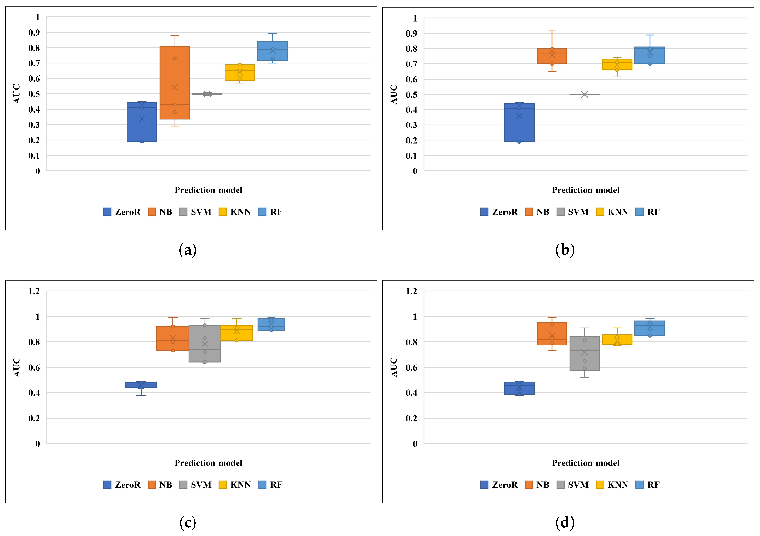
In this section, the results of the empirical study are presented and analyzed. Four prediction models involving three individual models (i.e., NB, SVM, and KNN) and one ensemble model (RF) were employed on seven datasets. Each prediction model was constructed using four different datasets extracted from the four scenarios analyzed (see Table 1). Therefore, the total number of prediction models was 112:7 datasets × 4 scenarios × 4 prediction models.

Figure 3 shows the box plots of the AUC of each prediction model across the seven datasets for the four scenarios (see Table 2). The mean value of the AUC values is indicated by an “X”, the upper and lower lines of the box represent the first and third quartile, and the middle horizontal line across the box represents the middle quartile. The prediction model which has the highest “X” values and the spread of the box is considered to be preferable. It is important to mention that because of the way that the scenarios were constructed, the test sets used for evaluating sampling methods in the third and fourth scenarios were different from those used for the non-sampling methods in the first and second scenarios. For this reason, the comparison between these two distinct groups of scenarios (first and second versus third and fourth) has not been carried out as it would be invalid. It is observed in Figure 3 that across all four scenarios, RF attained the highest prediction accuracy.

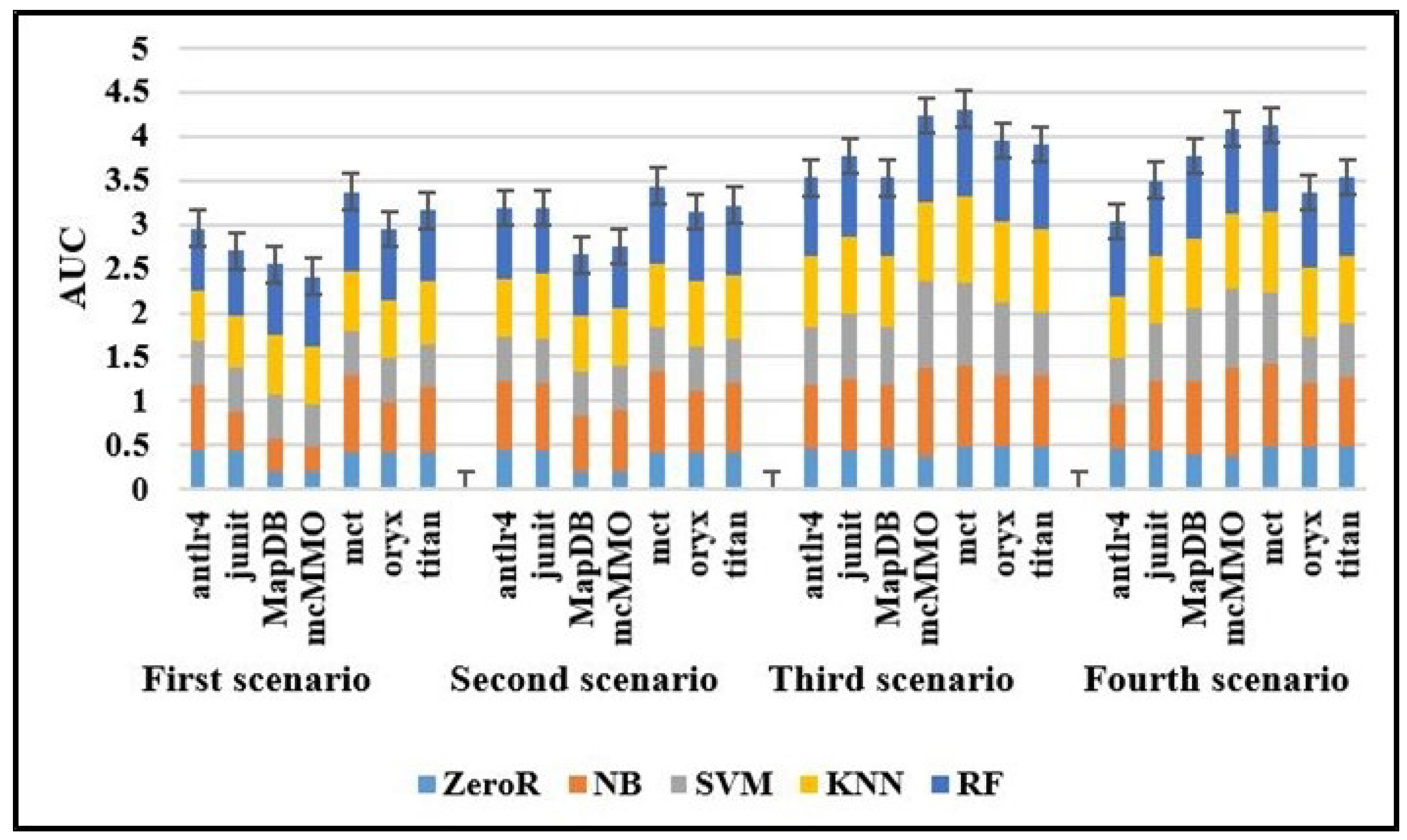
Figure 4 illustrates the AUC results obtained from each prediction model across seven datasets in four scenarios, in which the higher AUC value indicates the better result. The results of the third scenario provide valuable insights into the positive influence of ensemble sampling techniques to improve the prediction accuracy of prediction models. The basic findings are consistent with research showing that the sampling techniques improved the overall performance [8,9]. Regarding the overall results of the datasets, mcMMO and mct datasets achieved the highest prediction accuracy in both the third and fourth scenarios.

Table 12, Table 13, Table 14 and Table 15 present the results of AUC for prediction models across seven datasets in the first, second, third, and fourth scenarios, respectively. The prediction accuracy in terms of AUC measurement was evaluated, and the results of each scenario were presented separately in these tables considering the following aspects. First, the performance of the investigated prediction model was compared with the baseline, which is based on the dependent variable only (i.e., change-proneness) and predicts the mode value of this variable. Second, the best model in each dataset was identified (the highest AUC) using boldface. Third, the best model in all datasets was identified using boldface with underlined values. Finally, we investigate the impact of applying ensemble FS, sampling, and both ensemble FS and sampling techniques on the performance of prediction models, and the best model to predict change-proneness was determined.

5.3.1. Baseline

A baseline is provided in Table 12, Table 13, Table 14 and Table 15 for all scenarios. All the investigated models except NB in junit dataset in the first scenario (Table 15) achieved better prediction accuracy than the baseline. Consequently, these models have higher AUC values than those in the baseline model (i.e., ZeroR).

5.3.2. First Scenario: Datasets without FS or Sampling

Table 12 provides the results of AUC values for prediction models in seven datasets in the first scenario. These results indicate that RF outperformed all other prediction models, as RF provided higher AUC values in all datasets except antlr4, in which NB achieved a slightly better prediction accuracy (only 0.03 higher). KNN achieved the best performance among individual models and was the second-best prediction model.

Table 12. AUC values for performance evaluation of prediction models across seven datasets in the first scenario.

Models	Change-Proneness Dataset
	antlr4	junit	MapDB	mcMMO	mct	oryx	titan
First Scenario
ZeroR	0.45	0.44	0.19	0.19	0.41	0.41	0.41
NB	0.73	0.43	0.38	0.29	0.88	0.58	0.74
SVM	0.51	0.5	0.5	0.49	0.5	0.5	0.5
KNN	0.57	0.6	0.69	0.65	0.69	0.65	0.7
RF	0.7	0.73	0.79	0.79	0.89	0.81	0.81

Table 12. AUC values for performance evaluation of prediction models across seven datasets in the first scenario.

Models	Change-Proneness Dataset
	antlr4	junit	MapDB	mcMMO	mct	oryx	titan
First Scenario
ZeroR	0.45	0.44	0.19	0.19	0.41	0.41	0.41
NB	0.73	0.43	0.38	0.29	0.88	0.58	0.74
SVM	0.51	0.5	0.5	0.49	0.5	0.5	0.5
KNN	0.57	0.6	0.69	0.65	0.69	0.65	0.7
RF	0.7	0.73	0.79	0.79	0.89	0.81	0.81

5.3.3. Second Scenario: Datasets with FS and without Sampling

Table 13 presents the AUC values for prediction models across seven datasets in the second scenario. This scenario presents the prediction accuracy using ensemble FS mentioned in Section 4.1.4. Comparing the performance of the second scenario in Table 13 with that of the first scenario (without FS and sampling techniques) in Table 12, it is clear that FS improved the prediction accuracy in NB and KNN models except for one case (KNN in MapDB). In contrast, no impact was observed on SVM and RF compared to other prediction models. Additionally, FS produced either the same or an inferior performance to RF compared to the scenario without applying FS, except in antlr4 and junit. Although FS had no effect on RF, there was a clear competition between RF and NB to obtain the best prediction model in each dataset. Therefore, NB performed better than other individual models in terms of prediction accuracy, and achieved the best AUC value (0.92) in the mct dataset, which is considered outstanding according to the published criteria [52].

Table 13. AUC values for performance evaluation of prediction models across seven datasets in the second scenario.

Models	Change-Proneness Dataset
	antlr4	junit	MapDB	mcMMO	mct	oryx	titan
Second Scenario
ZeroR	0.45	0.44	0.19	0.19	0.41	0.41	0.41
NB	0.77	0.77	0.65	0.7	0.92	0.7	0.8
SVM	0.5	0.5	0.5	0.5	0.5	0.5	0.5
KNN	0.66	0.73	0.62	0.66	0.72	0.74	0.71
RF	0.81	0.75	0.7	0.7	0.89	0.8	0.8

Table 13. AUC values for performance evaluation of prediction models across seven datasets in the second scenario.

Models	Change-Proneness Dataset
	antlr4	junit	MapDB	mcMMO	mct	oryx	titan
Second Scenario
ZeroR	0.45	0.44	0.19	0.19	0.41	0.41	0.41
NB	0.77	0.77	0.65	0.7	0.92	0.7	0.8
SVM	0.5	0.5	0.5	0.5	0.5	0.5	0.5
KNN	0.66	0.73	0.62	0.66	0.72	0.74	0.71
RF	0.81	0.75	0.7	0.7	0.89	0.8	0.8

5.3.4. Third Scenario: Datasets without FS and with Sampling

Table 14 shows the AUC values for prediction models across seven datasets in the third scenario. This scenario provides the prediction accuracy using ensemble sampling techniques mentioned in Section 4.1.4. From Table 14, it is evident that the AUC values were extremely high. This good performance was achieved because the datasets were modified with sampling techniques proposed in Section 4.1.4 without applying FS. However, some features were excluded after applying data analysis. The most interesting finding from this scenario was that applying ensemble sampling techniques on the datasets that exclude improper features (i.e., features that have zero values and correlated with each other) in Section 4.1.3 is enough to reach a high prediction accuracy. Another notable result is that sampling techniques in third scenarios in Table 14 had a great impact on SVM. The result of SVM in the first and second scenarios was 0.5, which indicates no discrimination according to the published criteria [52]. Furthermore, RF achieved the best prediction accuracy in all datasets except NB in mcMMO, and RF in mct attained the close to optimal results of 0.99. KNN was the second-best prediction model and outperformed other individual models.

Table 14. AUC values for performance evaluation of prediction models across seven datasets in the third scenario.

Models	Change-Proneness Dataset
	antlr4	junit	MapDB	mcMMO	mct	oryx	titan
Third Scenario
ZeroR	0.46	0.44	0.46	0.38	0.49	0.48	0.48
NB	0.73	0.80	0.73	0.99	0.92	0.82	0.81
SVM	0.64	0.74	0.64	0.98	0.93	0.83	0.72
KNN	0.81	0.88	0.81	0.91	0.98	0.9	0.93
RF	0.89	0.92	0.89	0.98	0.99	0.92	0.97

Table 14. AUC values for performance evaluation of prediction models across seven datasets in the third scenario.

Models	Change-Proneness Dataset
	antlr4	junit	MapDB	mcMMO	mct	oryx	titan
Third Scenario
ZeroR	0.46	0.44	0.46	0.38	0.49	0.48	0.48
NB	0.73	0.80	0.73	0.99	0.92	0.82	0.81
SVM	0.64	0.74	0.64	0.98	0.93	0.83	0.72
KNN	0.81	0.88	0.81	0.91	0.98	0.9	0.93
RF	0.89	0.92	0.89	0.98	0.99	0.92	0.97

5.3.5. Fourth Scenario: Datasets with Both FS and Sampling

Table 15 provides the results of AUC for prediction models across seven datasets in the fourth scenario. This scenario lists the prediction accuracy using both the FS and sampling techniques. The main difference between the fourth scenario compared with the third scenario is using different metrics, but they used the same sampling method. Overall, the results of the fourth scenario indicate that the performance of machine learning models in most cases performed well. However, the results in this scenario are worse than the previous scenario. This suggests that applying both ensemble FS and sampling techniques decreased the prediction accuracy and using only sampling techniques was adequate to achieve high prediction accuracy. Again, RF outperformed other prediction models in all datasets except NB in mcMMO dataset, where the values of AUC range from 0.85 to 0.98, which is recognized as a good result. As in the first and second scenarios, KNN also was the second-best prediction model and performed better than other individual models.

Table 15. Scenarios in the empirical study.

Models	Change-Proneness Dataset
	antlr4	junit	MapDB	mcMMO	mct	oryx	titan
ZeroR	0.46	0.43	0.39	0.38	0.49	0.48	0.48
NB	0.51	0.79	0.84	0.99	0.94	0.73	0.8
SVM	0.51	0.65	0.82	0.91	0.81	0.52	0.59
KNN	0.71	0.78	0.78	0.84	0.91	0.78	0.77
RF	0.85	0.85	0.95	0.96	0.98	0.85	0.9

Table 15. Scenarios in the empirical study.

Models	Change-Proneness Dataset
	antlr4	junit	MapDB	mcMMO	mct	oryx	titan
ZeroR	0.46	0.43	0.39	0.38	0.49	0.48	0.48
NB	0.51	0.79	0.84	0.99	0.94	0.73	0.8
SVM	0.51	0.65	0.82	0.91	0.81	0.52	0.59
KNN	0.71	0.78	0.78	0.84	0.91	0.78	0.77
RF	0.85	0.85	0.95	0.96	0.98	0.85	0.9

5.3.6. Statistical Tests

We apply a one-way ANOVA to answer RQ4 by comparing all prediction models across four scenarios using AUC, where Factor A in the ANOVA test is the prediction model (NB, SVM, KNN, and RF). The results are shown in

Table 16. Scenarios in the empirical study.

Source	Sum of Squares	Degrees of Freedom	Mean Square	F	p-Value	Eta-Squared
Factor A	0.78	3.00	0.26	13.95	0.00	0.28
Error	2.02	108.00	0.02
Total	2.80	111.00

. We rejected H0 because all p-values in the table are less than $\alpha$ (0.05). According to the standards classifications of Cohen proposed in Section 4.3.2, the results of eta squared reveal that the effect size was large [57].

Additionally, multiple comparisons were performed using Tukey’s confidence intervals [53] (see Figure 5). In the chart, it is possible to identify which pairs of Factor A (prediction models) significantly differ across scenarios. If a confidence interval does not include 0, then the pair is significantly different. The results obtained from Figure 5 revealed that there were significant differences between ensemble models (RF) and all individual models (NB, SVM, and KNN). Similarly, there were significant differences between NB–SVM and SVM–KNN.

5.3.7. Impact of Parameter Tuning for Random Forests

In

Table 17. Scenario AUC values for performance evaluation of RF with default and Mtry parameter tuning.

Scenario	First			Second			Third			Fourth
	Mtry	AUC-T	AUC-D	Mtry	AUC-T	AUC-D	Mtry	AUC-T	AUC-D	Mtry	AUC-T	AUC-D
antlr4	3	0.81	0.7	2	0.84	0.81	6	0.94	0.89	1	0.87	0.85
junit	15	0.84	0.73	3	0.81	0.75	5	0.95	0.92	5	0.89	0.85
MapDB	2	0.90	0.79	10	0.72	0.7	8	0.96	0.89	2	0.98	0.95
mcMMO	11	0.89	0.79	2	0.89	0.7	6	1.00	0.98	5	0.98	0.96
mct	2	0.96	0.89	4	0.96	0.89	1	0.99	0.99	14	0.99	0.98
oryx	8	0.82	0.81	1	0.85	0.8	6	0.94	0.92	14	0.90	0.85
titan	8	0.90	0.81	6	0.85	0.8	15	0.99	0.97	2	0.93	0.9
Average	NA	0.87	0.79	NA	0.85	0.78	NA	0.97	0.94	NA	0.93	0.91
% of change	NA	10.13%		NA	8.97%		NA	3.19%		NA	2.20%

, the performance of AUC for RF with default parameters was compared with that of Mtry parameter tuning. Boldface values in the table highlight the best results among each dataset in each scenario, whereas AUC-T refers to the AUC for parameter tuning and AUC-D refers to the AUC for default parameters. The comparison of the results indicated that AUC-T outperformed AUC-D across all datasets in all scenarios, except mct dataset in the third scenario, which achieved the same result of AUC-D (0.99). AUC-T reached the optimal result (1.00) in the mcMMO dataset in the third scenario, and the average of AUC-T in all datasets in this scenario provided the highest prediction accuracy. Additionally, the grid search method provided different Mtry values for different datasets, which indicates that this method is an alternative to save time and effort instead of trying different parameters manually. The percentage of change between the average AUC-T and AUC-D across all datasets was 10.13%, 8.97%, 3.19%, and 2.20 in the first, second, third, and fourth scenarios, respectively. This indicates that tuning the Mtry parameter in RF had a positive influence in each scenario. However, this influence was higher in the original datasets (e.g., without FS or sampling in the first scenario) and lower in the edited datasets (e.g., with FS and sampling in the fourth scenario). Additionally, there is a good agreement between the findings in this section and those in the previous section, in which the third scenario achieved considerable performance.

5.3.8. Discussion and Answers to Research Questions

This section provides the discussion of the results presented above and answers the RQs for this study.

RQ1. What is the impact of ensemble FS techniques on the performance of prediction models?

Ensemble FS techniques in the second scenario improved the prediction accuracy of NB and KNN models. Analyzing the likely reasons behind this finding, firstly, NB is called naive because it creates conditional assumptions, which are independent from the features [37]. Second, using the Euclidean measure,

KNN determines the closest neighbors, which are also independent from the features [40]. Therefore, these models may have performed well with FS techniques because they do not perform attribute selection [45]. However, ensemble FS techniques had no clear impact on the overall performance of SVM and RF. This result may be explained by the fact that SVM algorithm includes the C parameter that selects the number of features, and the kernel function creates a suitable feature space [32]. Regarding the RF result, this occurs because RF has multiple decision trees that apply the same concept of FS using a top-down greedy search algorithm to choose the best feature at each step [58]. Therefore, SVM and RF algorithms already perform the FS concept during their creation. Additionally, RF includes many decision trees, which perform adequately with an imbalanced dataset because they tend to build several tests to recognize the difference between the minority and majority classes [59]. For this reason, RF achieved the best prediction accuracy in the second scenario.

RQ2. What is the impact of ensemble sampling techniques on the performance of prediction models?

The machine learning models with ensemble sampling techniques achieved good performance. Again, RF achieved the best results of AUC values across all the datasets except mcMMO. These findings may help us to conclude that performing ensemble sampling techniques and removing inappropriate features in the data analysis step without applying ensemble FS is sufficient to predict change proneness accurately. This is consistent with what has been found in a series of recent studies [8,9] that used several types of sampling techniques: SMOTE [8], UPSAMPLE, SMOTE and RUSBoost [9], and emphasizes the effect of these techniques to improve the performance of the prediction models.

Interestingly, ensemble sampling techniques in this particular case increased the prediction accuracy of SVM and RF. This supports the findings in the previous question indicting that SVM and RF algorithms can deal with FS during their creation. Consequently, these algorithms respond to sampling techniques more than FS techniques.

RQ3. What is the impact of applying both ensemble FS and sampling techniques on the performance of prediction models?

Applying both ensemble FS and sampling techniques improved the performance of the prediction models, and RF achieved the best performance across all datasets except mcMMO. These findings corroborate the ideas of Kumar and Sureka, who used the same datasets to predict refactoring and performed principal component analysis and SMOTE techniques to extract the best features and resolve the imbalanced data problem [8]. Their results indicated that the prediction accuracy with the SMOTE technique was better than that without SMOTE, and the prediction accuracy of all metrics was better than that with FS. A possible explanation for these results may be the lack of adequate datasets, and the rank of the best ten features selected is considered low (the average ranking of the best ten metrics ranges from 0.1 to 0.6), whereas the difference before and after applying sampling techniques is high (see Table 10 and Table 11).

RQ4. What is the performance of the individual model and do the ensemble models (i.e., RF) outperform individual models?

KNN achieved the best prediction accuracy among most cases. RF outperformed other individual models and achieved the best result in terms of average AUC value (see Figure 3) across all scenarios. The results of the ANOVA test reveal that there were significant differences between RF and all individual models (see Figure 5). In addition, the results of the effect size were large (see Table 16). Therefore, applying ensemble sampling techniques on RF produced the highest accuracy to predict change-proneness. This finding is in accordance with previous studies, in which RF provided the best performance to predict change-proneness [4], software faults [60], and maintenance changes [61].

RQ5. What is the impact of the Mtry parameter tuning in RF?

Mtry parameter tuning in RF using grid search method, along with RF, mlbench, and caret packages, improved prediction accuracy. This improvement increased in the original datasets (e.g., without FS or sampling) and decreased in the edited datasets (e.g., with FS and sampling in the fourth scenario). The findings of this RQ are consistent with those of Fernández-Delgado et al., who stated that RF created using caret package in R was the best model among 179 models applied on 121 original datasets [62]. Furthermore, the Mtry parameter differed from various datasets, and this difference was behind the study showing that there are no suggestions to choose the specific number of the Mtry parameter [26]. In addition, this supports the use of automatic parameters tuning to simply and effectively improve performance [63,64]. Based on these findings, it is recommended to tune the Mtry parameter automatically to save time and efforts and improve the results. In future work, a statistical test will be used to investigate the performance difference between RF without and with parameter tuning.

6. Threats to Validity

The threats to validity usually emerge in any experimental software engineering study [65]. This section describes the threats to validity using four categories: external, conclusion, internal, and constructed, and also provides an explanation of how they are resolved and handled.

6.1. External Validity

External validity indicates the degree of generalization of results outside the empirical study setting [65]. Publicly available datasets extracted from open-source software systems were used to enable reprehensibility and comparison with other empirical studies that used the same datasets. However, these datasets were collected from only a particular programming language (i.e., Java), and therefore additional research requires to be conducted for other programming languages (e.g., C++ and C#). Moreover, we believe that the datasets used in this study are likely to be valid in terms of the number of classes and number of releases. We also emphasize that the application of the results can be generalized by considering other releases of the same projects or using method level instead of the class level that used in this study. Additionally, the ensemble FS and sampling techniques used in this study can be easily implemented to other change-proneness datasets.

6.2. Conclusion Validity

Conclusion validity relates to the statistical relationship between the results and the output of the experiment, which impacts on the capability to reach the right conclusion [66]. To avoid the threat of conclusion validity, ten-fold cross validation was performed to reduce potentially biased results by selecting tests from the entire dataset. This validation is repeated ten times to generate statistically reliable results and avoid the conclusion threat. In addition, we only used AUC to evaluate and compare the prediction models because AUC is more effective for imbalanced datasets than other measurements (e.g., precision or recall). Moreover, the conclusions are dependent on statistical tests for significance. We used ANOVA test, which is a parametric statistical test that requires some assumptions, such as normal distribution for the datasets and independent observations of each other. However, these assumptions were met and one of the main advantages of the parametric statistical test is to provide more reliable results with both non-normally and continuous datasets. Hence, the threat to conclusion validity may exist due to using a parametric statistical test.

6.3. Internal Validity

Internal validity is the ability to present the results with different experimental variables [66]. In order to prevent threat of internal validity, we explore the effectiveness of ensemble FS and sampling techniques on the performance of the prediction models using several source code metrics across four scenarios. Nevertheless, evaluating the impact of each metric on predicting change-proneness was outside the scope of this study but could be explored as future work. Four prediction models were built, and these models were the most frequently used in [7] and appropriate for classification problems. In addition, Weka, which is an established and frequently employed tool, is used to select features, perform sampling, and build prediction models [41]. Therefore, there are no threats to internal validity in term of selection of prediction models and tool.

6.4. Construct Validity

Construct validity measures the relationship between the dependent and independent variables [67]. In this study, we create machine learning models depending on 125 metrics that were manually validated and extracted from class-level to capture several features of the software product [13]. Some of these metrics were eliminated before conducting empirical study (see Section 4.1) and some of them were removed by applying data analysis and ensemble FS in Section 4.1.3 and Section 4.1.4, respectively. However, many of these metrics are used for the first time to predict change-proneness and we can conclude that the metrics used in this study are investigated recently, so there is threat to construct validity of these metrics. Furthermore, other validity concerns relate to the dependent variable (i.e., change-proneness), which is a Boolean variable that reflects changes of refactoring (i.e., changes of the structure of the internal source code without affecting the functionality of source code [8]). The prediction of change-proneness variable has been investigated in several studies and it is considered as good indicator [5,15]. However, this study did not recognize the types of changes (i.e., adaptive, corrective, preventive, or perfective). Therefore, we are aware that this can threaten the construct validity of the dependent variable. However, we still used change-proneness as a dependent variable as recommended by [2], because limited studies considered the types of the change proneness [4].

7. Conclusions and Future Work

Ensemble FS and sampling techniques play a vital role for improving the prediction accuracy of machine learning models. However, the application of these techniques on software maintainability is limited. In this study, we apply three individual models, NB, SVM, and KNN, along with one ensemble model, RF, on seven publicly available datasets collected from open-source software systems. We evaluated and compared the effectiveness of ensemble FS and ensemble sampling techniques on the performance of prediction change-proneness. This study presents many insights, which are based on comprehensive experimentation and analyses:

• The results obtained from this study provide empirical evidence of the positive impact of ensemble FS in improving the performance of some of the prediction models (KNN and NB). However, ensemble FS techniques had no clear effect on the overall performance of SVM and RF because these models have FS techniques as a part of the model’s creation.
• This study also showed the good performance of applying ensemble sampling methods on all prediction models and that there was a clear improvement in SVM and RF.
• Across all scenarios, the ensemble model (RF) achieved the best performance in predicting change-proneness compared to other models, and there were significant differences between RF and all individual models. In addition, the effect size was large. A possible explanation of the good performance of RF in both high-dimensional and imbalanced datasets is that RF performs the concept of FS through the creation of several decision trees. It also involves many decision trees that perform well with the imbalanced dataset.
• The experimental results in this empirical study showed that the performance of the ensemble models for predicting change-proneness is significantly improved, and the effect size was large in all prediction models.

Indeed, the results obtained from this study provide empirical evidence of the positive impact of ensemble FS and sampling techniques in improving the performance of the prediction models to predict change-proneness. We observed that the ensemble model (RF) achieved the best performance in predicting change-proneness compared to other models. Moreover, the proposed ensemble FS and sampling techniques improved the prediction accuracy of change-proneness. In future work, we will investigate the combination of different FS and sampling techniques to achieve more consistent results. Moreover, we will employ different prediction models on various software maintainability datasets, and the study can also be extended to recognize the most suitable metrics to indicate change-proneness.

References

- Alsolai, H. Predicting Software Maintainability in Object-Oriented Systems Using Ensemble Techniques. In Proceedings of the 2018 IEEE International Conference on Software Maintenance and Evolution (ICSME), Madrid, Spain, 23–29 September 2018; pp. 716–721. [Google Scholar]
- Koru, A.; Tian, J. Comparing high-change modules and modules with the highest measurement values in two large-scale open-source products. IEEE Trans. Softw. Eng. 2005, 31, 625–642. [Google Scholar] [CrossRef]
- Alsolai, H.; Roper, M. A Systematic Literature Review of Machine Learning Techniques for Software Maintainability Prediction. Inf. Softw. Technol. 2020, 119, 106214. [Google Scholar] [CrossRef]
- Catolino, G.; Ferrucci, F. An extensive evaluation of ensemble techniques for software change prediction. J. Softw. Evol. Process 2019, 31, 1–15. [Google Scholar] [CrossRef]
- Malhotra, R.; Khanna, M. Particle Swarm Optimization-Based Ensemble Learning for Software Change Prediction. Inf. Softw. Technol. 2018, 102, 65–84. [Google Scholar] [CrossRef]
- Nucci, D.; Palomba, F.; Oliveto, R.; Lucia, A. Dynamic Selection of Classifiers in Bug Prediction: An Adaptive Method. IEEE Trans. Emerg. Top. Comput. Intell. 2017, 1, 202–212. [Google Scholar] [CrossRef]
- Alsolai, H.; Roper, M. A Systematic Review of Feature Selection Techniques in Software Quality Prediction. In Proceedings of the International Conference on Electrical and Computing Technologies and Applications, Ras Al Khaimah, United Arab Emirates, 19–21 November 2019; pp. 1–5. [Google Scholar]
- Kumar, L.; Sureka, A. Application of LSSVM and SMOTE on Seven Open Source Projects for Predicting Refactoring at Class Level. In Proceedings of the Asia-Pacific Software Engineering Conference, Nanjing, China, 4–8 December 2017; pp. 90–99. [Google Scholar]
- Kumar, L.; Satapathy, S.; Murthy, L. Method Level Refactoring Prediction on Five Open Source Java Projects using Machine Learning Techniques. In Proceedings of the India Software Engineering Conference, Pune, India, 14–16 February 2019; pp. 1–10. [Google Scholar]
- Loyola-González, O.; García-Borroto, M.; Medina-Pérez, M.; Martínez-Trinidad, J.; Carrasco-Ochoa, J.; Ita, G. An Empirical Study of Oversampling and Undersampling Methods for Lcmine An Emerging Pattern Based Classifier. In Mexican Conference on Pattern Recognition; Springer: Berlin/Heidelberg, Germany, 2013; pp. 264–273. [Google Scholar]
- Khoshgoftaar, T.; Gao, K.; Napolitano, A.; Wald, R. A Comparative Study of Iterative and Non-Iterative Feature Selection Techniques for Software Defect Prediction. Inf. Syst. Front. 2014, 16, 801–822. [Google Scholar] [CrossRef]
- Liu, Y.; An, A.; Huang, X. Boosting Prediction Accuracy on Imbalanced Datasets with SVM Ensembles; Springer: Berlin/Heidelberg, Germany, 2006. [Google Scholar]
- Hegedűs, P.; Kádár, I.; Ferenc, R.; Gyimóthy, T. Empirical Evaluation of Software Maintainability Based on a Manually Validated Refactoring Dataset. Inf. Softw. Technol. 2018, 95, 313–327. [Google Scholar] [CrossRef]
- Cukic, B. Guest Editor’s Introduction: The Promise of Public Software Engineering Data Repositories. IEEE Softw. 2005, 22, 20–22. [Google Scholar] [CrossRef]
- Elish, M.; Al-Khiaty, M. A suite of metrics for quantifying historical changes to predict future change-prone classes in object-oriented software. J. Softw. Evol. Process 2013, 25, 407–437. [Google Scholar] [CrossRef]
- Chidamber, S.; Kemerer, C. Towards a Metrics Suite for Object Oriented Design. In Proceedings of the Conference Proceedings on Object-Oriented Programming Systems, Languages, and Applications, Phoenix, AZ, USA, 6–11 October 1991; pp. 197–211. [Google Scholar]
- Malhotra, R.; Khanna, M. Inter Project Validation for Change Proneness Prediction using Object Oriented Metrics. Softw. Eng. Int. J. 2013, 3, 21–31. [Google Scholar]
- Malhotra, R.; Khanna, M. Investigation of relationship between object-oriented metrics and change proneness. Int. J. Mach. Learn. Cybern. 2013, 4, 273–286. [Google Scholar] [CrossRef]
- Kumar, L.; Rath, S.; Sureka, A. Empirical analysis on effectiveness of source code metrics for predicting change-proneness. In Proceedings of the 10th Innovations in Software Engineering Conference, Jaipur, India, 5–7 February 2017; pp. 4–14. [Google Scholar]
- Lu, H.; Zhou, Y.; Xu, B.; Leung, H.; Chen, L. The Ability of Object-Oriented Metrics to Predict Change-Proneness: A Meta-Analysis. Empir. Softw. Eng. 2012, 17, 200–242. [Google Scholar] [CrossRef]
- Ueda, N.; Nakano, R. Generalization Error of Ensemble Estimators. Proceedings of International Conference on Neural Networks 1996, Washington, DC, USA, 3–6 June 1996; Volume 1, pp. 90–95. [Google Scholar]
- Wang, T.; Li, W.; Shi, H.; Liu, Z. Software defect prediction based on classifiers ensemble. J. Inf. Comput. Sci. 2011, 8, 4241–4254. [Google Scholar]
- Zhang, Y.; Lo, D.; Xia, X.; Sun, J. An Empirical Study of Classifier Combination for Cross-Project Defect Prediction. In Proceedings of the Annual Computer Software and Applications Conference, Taichung, Taiwan, 1–5 July 2015; pp. 264–269. [Google Scholar]
- Minku, L.; Yao, X. Ensembles and Locality: Insight on Improving Software Effort Estimation. Inf. Softw. Technol. 2013, 55, 1512–1528. [Google Scholar] [CrossRef] [Green Version]
- Azzeh, M.; Nassif, A.; Minku, L. An Empirical Evaluation of Ensemble Adjustment Methods for Analogy-Based Effort Estimation. J. Syst. Softw. 2015, 103, 36–52. [Google Scholar] [CrossRef] [Green Version]
- Scornet, E. Tuning Parameters in Random Forests. ESAIM 2017, 60, 144–162. [Google Scholar] [CrossRef] [Green Version]
- Github. The Largest Open Source Community in The World. Available online: https://github.com/ (accessed on 5 May 2017).
- SourceMeter Static Code Analysis Tool. Available online: https://www.sourcemeter.com/resources/java/ (accessed on 8 June 2019).
- Briand, L.; Wüst, J.; Daly, J.; Porter, D. Exploring the Relationships Between Design Measures and Software Quality in Object-Oriented Systems. J. Syst. Softw. 2000, 51, 245–273. [Google Scholar] [CrossRef]
- Corder, G.; Foreman, D. Nonparametric Statistics: A Step-by-Step Approach; Wiley: Hoboken, NJ, USA, 2014; p. 288. [Google Scholar]
- Badr, W. Why Feature Correlation Matters...A Lot! Available online: https://towardsdatascience.com/why-feature-correlation-matters-a-lot-847e8ba439c4 (accessed on 6 May 2020).
- Han, J.; Pei, J.; Kamber, M. Data Mining: Concepts and Techniques; Elsevier: Amsterdam, The Netherlands, 2011; p. 744. [Google Scholar]
- Gao, K.; Khoshgoftaar, T.; Wald, R. Combining Feature Selection and Ensemble Learning for Software Quality Estimation. In Proceedings of the International Florida Artificial Intelligence Research Society Conference, Beach, FL, USA, 21–23 May 2014; pp. 47–52. [Google Scholar]
- Brownlee, J. Machine Learning Mastery with Weka; Ebook, Ed.; Available online: https://machinelearningmastery.com/machine-learning-mastery-weka/ (accessed on 9 July 2019).
- Chawla, N. Data Mining for Imbalanced Datasets: An Overview. In Data Mining and Knowledge Discovery Handbook; Springer: Berlin/Heidelberg, Germany, 2009; pp. 875–886. [Google Scholar]
- Wolff, R. Classification Algorithms in Machine Learning: How They Work. Available online: https://monkeylearn.com/blog/classification-algorithms/ (accessed on 7 April 2020).
- John, G.; Langley, P. Estimating Continuous Distributions in Bayesian Classifiers. In Proceedings of the Conference on Uncertainty in Artificial Intelligence, Montreal, QC, Canada, 18–20 August 1995; pp. 338–345. [Google Scholar]
- Shevade, S.; Keerthi, S.; Bhattacharyya, C.; Murthy, K. Improvements to the SMO algorithm for SVM regression. IEEE Trans. Neural Netw. 2000, 11, 1188–1193. [Google Scholar] [CrossRef] [Green Version]
- Awad, M.; Khanna, R. Support Vector Regression. In Efficient Learning Machines: Theories, Concepts, and Applications for Engineers and System Designers; Apress: Berkeley, CA, USA, 2015; pp. 67–80. [Google Scholar]
- Aha, D.; Kibler, D.; Albert, M. Instance-Based Learning Algorithms. Mach. Learn. 1991, 6, 37–66. [Google Scholar] [CrossRef] [Green Version]
- Witten, I.; Frank, E.; Trigg, L.; Hall, M.; Holmes, G.; Cunningham, S. Weka: Practical Machine Learning Tools and Techniques with Java Implementations; University of Waikato, Department of Computer Science: Hamilton, New Zealand, 1999. [Google Scholar]
- Aher, S.; Lobo, L. Data Mining in Educational System Using Weka. In Proceedings of the International Conference on Emerging Technology Trends, Kollam, India, 21–22 October 2016; Volume 3, pp. 20–25. [Google Scholar]
- Venkatesh, A.; Jacob, S. Prediction of Credit-Card Defaulters: A Comparative Study on Performance of Classifiers. Int. J. Comput. Appl. 2016, 145, 36–41. [Google Scholar]
- Mean Median Mode Formula. Available online: https://www.cuemath.com/mean-median-mode-formula/ (accessed on 25 March 2022).
- Gao, K.; Khoshgoftaar, T.; Wang, H.; Seliya, N. Choosing Software Metrics for Defect Prediction: An Investigation on Feature Selection Techniques. Softw. Pract. Exp. 2011, 41, 579–606. [Google Scholar] [CrossRef] [Green Version]
- Zhi-Qiang, Z.; Hong-Bin, Y.; Hua-Rong, X.; Yan-Qi, X.; Ji, G. Fast Training Support Vector Machines Using Parallel Sequential Minimal Optimization. In Proceedings of the International Conference on Intelligent System and Knowledge Engineering, Xiamen, China, 17–19 November 2008; Volume 1, pp. 997–1001. [Google Scholar]
- Freund, Y.; Schapire, R. Experiments With A New Boosting Algorithm. In Proceedings of the International Conference on International Conference on Machine Learning, Bari, Italy, 3–6 July 1996; pp. 148–156. [Google Scholar]
- Breiman, L. Random Forests. Mach. Learn. 2001, 45, 5–32. [Google Scholar] [CrossRef] [Green Version]
- Hall, M.; Frank, E.; Holmes, G.; Pfahringer, B.; Reutemann, P.; Witten, I. The WEKA Data Mining Software: An Update. ACM SIGKDD Explor. Newsl. 2009, 11, 10–18. [Google Scholar] [CrossRef]
- Conte, S.; Dunsmore, H.; Shen, V. Software Engineering Metrics and Models; Benjamin-Cummings Publishing Co., Inc.: San Francisco, CA, USA, 1986; p. 396. [Google Scholar]
- Bradley, A. The Use of the Area Under the ROC Curve in the Evaluation of Machine Learning Algorithms. Pattern Recognit. 1997, 30, 1145–1159. [Google Scholar] [CrossRef] [Green Version]
- Hosmer, D., Jr.; Lemeshow, S.; Sturdivant, R. Applied Logistic Regression; John Wiley & Sons: Hoboken, NJ, USA, 2013; p. 528. [Google Scholar]
- Berenson, M.; Levine, D.; Goldstein, M. Intermediate Statistical Methods and Applications: A Computer Package Approach; Prentice-Hall, Inc.: Hoboken, NJ, USA, 1983; p. 579. [Google Scholar]
- Lakens, D. Calculating and Reporting Effect Sizes to Facilitate Cumulative Science: A Practical Primer for T-Tests and ANOVAs. Front. Psychol. 2013, 4, 863. [Google Scholar] [CrossRef] [Green Version]
- Cohen, J. Statistical Power Analysis for the Behavioral Sciences; Routledge: London, UK, 2013. [Google Scholar]
- Osman, H.; Ghafari, M.; Nierstrasz, O. Hyperparameter Optimization to Improve Bug Prediction Accuracy. In Proceedings of the Workshop on Machine Learning Techniques for Software Quality Evaluation 2017, Klagenfurt, Austria, 21–21 February 2017; pp. 33–38. [Google Scholar]
- Cohen, J. A Power Primer. Psychol. Bull. 1992, 112, 155. [Google Scholar] [CrossRef]
- He, H.; Garcia, E. Learning from Imbalanced Data. IEEE Trans. Knowl. Data Eng. 2009, 21, 1263–1284. [Google Scholar]
- Batista, G.; Prati, R.; Monard, M. A Study of the Behavior of Several Methods for Balancing Machine Learning Training Data. ACM SIGKDD Explor. Newsl. 2004, 6, 20–29. [Google Scholar] [CrossRef]
- Catal, C.; Diri, B. Investigating the Effect of Dataset Size, Metrics Sets, and Feature Selection Techniques on Software Fault Prediction Problem. Inf. Sci. 2009, 179, 1040–1058. [Google Scholar] [CrossRef]
- Kaur, A.; Kaur, K.; Pathak, K. Software Maintainability Prediction by Data Mining of Software Code Metrics. In Proceedings of the International Conference on Data Mining and Intelligent Computing, Delhi, India, 5–6 September 2014; pp. 1–6. [Google Scholar]
- Fernandez-Delgado, M.; Cernadas, E.; Barro, S.; Amorim, D. Do we need hundreds of classifiers to solve real world classification problems? J. Mach. Learn. Res. 2014, 15, 3133–3181. [Google Scholar]
- Fu, W.; Menzies, T.; Shen, X. Tuning for Software Analytics: Is it Really Necessary? Inf. Softw. Technol. 2016, 76, 135–146. [Google Scholar] [CrossRef] [Green Version]
- Tantithamthavorn, C.; McIntosh, S.; Hassan, A.; Matsumoto, K. Automated Parameter Optimization of Classification Techniques for Defect Prediction Models. In Proceedings of the International Conference on Software Engineering 2016, Austin, TX, USA, 14–22 May 2016; pp. 321–332. [Google Scholar]
- Wright, H.; Kim, M.; Perry, D. Validity Concerns in Software Engineering Research. In Proceedings of the FSE/SDP Workshop on Future of Software Engineering Research, Santa Fe, NM, USA, 7–8 November 2010; pp. 411–414. [Google Scholar]
- Khoshgoftaar, T.; Seliya, N.; Sundaresh, N. An Empirical Study of Predicting Software Faults with Case-Based Reasoning. Softw. Qual. J. 2006, 14, 85–111. [Google Scholar] [CrossRef]
- Pai, G.; Dugan, J. Empirical Analysis of Software Fault Content and Fault Proneness Using Bayesian Methods. IEEE Trans. Softw. Eng. 2007, 33, 675–686. [Google Scholar] [CrossRef]