
Automatic Intersection Extraction Method for Urban Road Networks Based on Trajectory Intersection Points


1
Beijing Key Laboratory of Urban Road Traffic Intelligent Control Technology, North China University of Technology, Beijing 100144, China
2
School of Information Science and Technology, North China University of Technology, Beijing 100144, China
*
Author to whom correspondence should be addressed.
Appl. Sci. 2022, 12(12), 5873; https://0-doi-org.brum.beds.ac.uk/10.3390/app12125873
Submission received: 23 March 2022
/
Revised: 20 May 2022
/
Accepted: 6 June 2022
/
Published: 9 June 2022
(This article belongs to the Special Issue Transportation Big Data and Its Applications)
Abstract
:Automatic intersection identification and extraction are an important foundation for urban road network updates and traffic network analysis and modeling. Existing intersection extraction methods based on steering angles and stopping points suffer from inadequate sampling amounts and threshold settings. To address this problem, we propose a road network intersection automatic extraction method based on vehicle trajectory intersection clustering. First, the continuous trajectory segments are extracted from trajectory data based on the sampling interval. Second, the maximum reconstruction error method is developed to extract straight-line trajectory segments from continuous trajectory segments. The overlapped straight-line trajectory segments belonging to the same direction are merged to reduce the number of segments and enhance road network patterns. To further improve the calculation efficiency of the intersection points of straight-line segments, bounding box filtering and orthogonal filtering are used to filter the straight-line trajectory segments that do not have an intersection relationship. Finally, the obtained straight-line segment intersection points are clustered using a density peak clustering algorithm. The road intersections are automatically extracted using the clustering center. The experimental results on real vehicle trajectories in Lianyungang City show that the proposed method performs well on intersection recognition and calculation efficiency.
1. Introduction
Intersections are important junctions of urban traffic road networks, as well as bottlenecks of traffic flow and key nodes of urban traffic management. The automatic extraction and identification of intersection location and structure are of fundamental importance for road network map updates, network traffic flow analysis, urban traffic management, and critical path identification. Existing extraction research on intersections mostly relies on data sources such as remote sensing images [1], historical map images [2], multi-sensor combinations, GPS trajectory data, and so on. Among them, methods based on remote sensing images are sensitive to factors such as weather, lighting, and road environment, resulting in inaccurate intersection processing. Methods based on multi-sensor combinations are limited by the spatial coverage of the sensors and are only effective within a certain range.
With the rapid development of intelligent vehicle terminals, autonomous driving, and 5G communication technology, vehicle GPS trajectory data are becoming more accessible, with higher accuracy and richer feature information. Mousavizadeh et al. [3] estimate the real-time vehicle turning rate using floating car data in road intersections. Sun et al. [4] predict traffic congestion based on GPS trajectory using a deep learning method. Tang et al. [5] present an automatic method for the detection and update of newly added roads based on the common low-quality trajectory data. The authors used a point-to-segment matching algorithm to acquire line segment road network structure but did not take advantage of trajectory information. Wang et al. [6] used low-sample frequency data to reconstruct vehicle trajectories through road intersections. The trajectory was adjusted microscopically using a probability method; these studies all focus on intersections as the core area. The location extraction and structure recognition of road network intersections based on trajectory data is the first part or kernel problem of such studies, and it is increasingly becoming a current research hotspot.
By using trajectory data, the intersection extraction is based on the characteristics of trajectories within the intersection area. There is much literature on intersection extraction by clustering the characteristics of each sampling point in a single trajectory. The widely used characteristic is the steering angle, which is used by Deng et al. [7] and Tang et al. [8]. Some studies try to use different clustering algorithms to improve performance. Wang et al. [9] used a mean-shift algorithm for the clustering steering angle. Hu et al. [10] detected the traffic intersection using floating car data; they used the angle of the direction difference for detecting the traffic intersection, and a density clustering algorithm (DBSCAN) for identifying traffic intersections. Gao et al. [11] improved the density peak clustering algorithm. Some studies enhance the steering point feature by integrating multiple features. Huang et al. [12] detected road intersections from large-scale vehicle trajectories by clustering turning points and then removing the false detections using direction discrepancy and turning discrepancy. Chen et al. [13] detected road intersections by proposing a novel turn-point position compensation in order to improve the concentration of selected turn-points under low sampling rates, and indeed there are also studies using other single-trajectory characteristics. Zourlidou et al. [14] determined the location and area of the intersection using density-based clustering on vehicle stop points. Zhou et al. [15] proposed a geospatial method to extract functionally critical network location (FCNL) as road intersections from trajectories. The FCNL has multiple characterizations, such as a large number of activity trajectories, and is traversed by trajectories exhibiting diverse patterns; however, among the existing research, the intersection extraction method based on characteristics of the single trajectory is influenced by the trajectory sampling amount, which is leading to ignoring road intersections with low sampling amounts.
There are also some studies based on the properties of multiple trajectories within the grid of a small area; C.Wang et al. [16] extracted an intersection and stop bar from crowdsourced GPS trajectories. They gridded the target area and calculated the entropy of the moving direction within each grid to identify intersection areas. Keler et al. [17] introduced a method for intersecting vehicle trajectories and extracting their intersection points for selected rush hours in urban environments. In J.Wang [18]’s study on generating routable road maps from vehicle GPS traces, the authors detected conflict points in the grid and clustered these trajectory conflict points to extract road intersection information. Fathi et al. [19] introduced a local shape descriptor to represent the distribution of the GPS trajectory in a circular area and constructed an intersection detector based on the local shape descriptor by introducing an intersection detector that uses a localized shape descriptor to represent the distribution of GPS traces around a point. Although the methods based on grids are less influenced by the sample amount, the grid size is difficult to determine when facing the uneven distribution of trajectory density in a large-scale road network. One study attempted to automatically set up grids. Zhao et al. [20] proposed an automatic calibration method for road intersection topology using trajectories and determined the location and coverage of road intersections by employing a top-down quad-tree-based cell division method; however, the geometric structure relationship between trajectories has not been effectively utilized. Li et al. [21] proposed a regularized mean-shift algorithm to refine GPS scattered points and road segments were extracted from these refined points to represent road network structure. In our approach, however, we extract straight-line segments from each single trajectory directly.
We propose an intersection extraction method from GPS trajectory data. Compared to previous work in this field, our method directly extracts straight-line segments from each single trajectory. Then, we use the intersection points of all straight-line segments to identify road intersections. The algorithm for separating line segments from GPS trajectories is an important part of our approach.
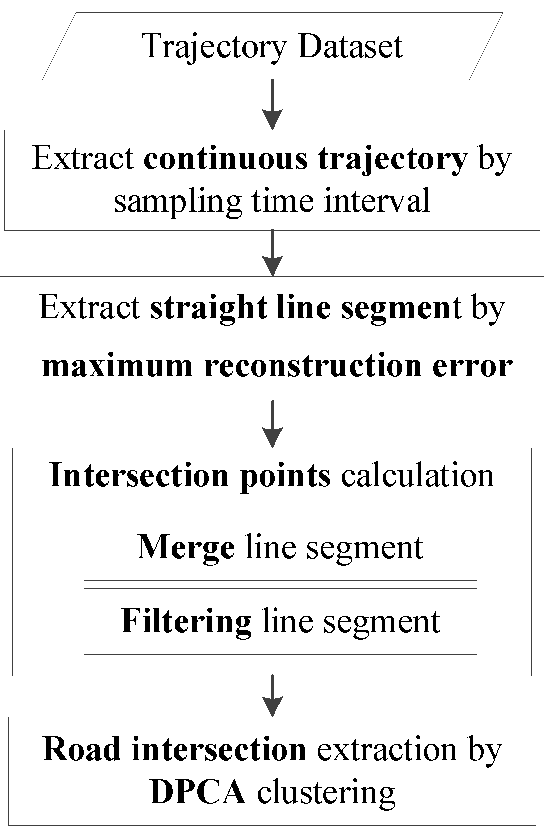
The intersection points of vehicle straight-line trajectories mostly occur in road intersection areas. We use the geometrical structure of the road network carried by the trajectory and propose an intersection extraction method based on clustering the trajectory straight-line segment intersection points. The workflow for extracting road intersections is shown in Figure 1.
First, the original trajectory dataset is segmented according to sampling time interval to extract spatial–temporal continuous trajectories. Second, the maximum reconstruction error method is proposed to extract straight-line trajectory segments from spatial–temporal continuous trajectories. The overlapped straight-line segments belonging to the same direction are merged to reduce the number of segments and enhance the straight-line road pattern. The amount of calculation at the intersection of a straight-line segment is significantly reduced by bounding box overlapping filtering and orthogonal filtering. The intersection points are calculated for any two filtered straight-line segments. Finally, the intersection points are clustered using the density peaking algorithm [22] and the cluster centers are used as the location of the intersections. The proposed method was verified using real trajectory data in Lianyungang City in China and the experimental results show that this method can automatically extract intersection locations effectively and efficiently.
The following section provides the proposed method. Section 2.1 provides a continuous trajectory segment extraction. Section 2.2 gives a detailed description of the algorithm for the extraction of straight trajectory segments using the maximum reconstruction error. Section 2.3 and Section 2.4 describe the method for calculating the intersection point and extracting intersection information by clustering. Experimental results and discussions are presented in Section 3. Conclusions are given in Section 4.
2. Proposed Method
2.1. Continuous Trajectory Extraction
To better illustrate the method of this paper, the following basic definitions are given.
Definition 1.
Location point: A tuple consisting of latitude and longitude, which represents the spatial location of a vehicle and is denoted by, where x is longitude and y is latitude.
Definition 2.
Trajectory sampling points: A tuple is formed by adding the vehicle identifier vid and sampling time t to the location points, denoted by.
Definition 3.
Trajectory: A sequence of all trajectory sampling points of a vehicle within a certain period of time in the order of the sampling time, denoted as , where represents the amount of sampling points contained in a given trajectory T.
Definition 4.
Continuous trajectory: A sub-trajectory of a trajectory T, which satisfies the sampling interval of adjacent trajectory sampling points less than a given threshold , is denoted as
satisfyingfor any adjacent sampling pointsand.
Due to some large sampling time intervals existing in the original trajectory data, which leads to a reduction in the trajectories’ confidence, the original trajectory needs to be divided by the location points with large sampling time intervals to obtain a continuous trajectory.
When dividing the original trajectory, it is important to select a proper sampling time interval threshold. A sampling time interval threshold that is too large will retain some original trajectories with a large sampling interval, thus reducing the effectiveness of the segmentation. A threshold that is too small will make the divided trajectory segments too fragmented and risk losing the original trajectory information.
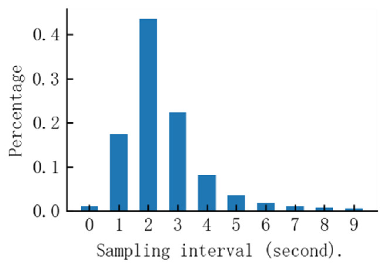
Therefore, it is necessary to set a sampling time interval threshold for continuous trajectories based on prior experience and the distribution characteristics of the experimental data. In this paper, the dataset is BaiduMap’s vehicle trajectory data in Lianyungang City in China. The general GPS sampling interval of this navigation map is 2 s. The distribution of the sampling time interval of all the sampling points of the dataset used in this paper is shown in Figure 2.
As can be seen from Figure 2, most of the original trajectory data sampling time interval is less than 5 s; therefore, we set the continuous trajectory sampling time interval threshold to 5 s and about 95% of all sampling points. The continuous trajectory amount after segmentation by this threshold is about 10 times the original trajectory amount.
After time interval segmentation, on the other hand, there are trajectories with few sampling points (short trajectories) in the segmented continuous trajectory segment. These short trajectories should be removed as noise to obtain a valid continuous trajectory, and are removed according to the amount of sampling points. When the number of sampling points of a continuous trajectory is less than a preset threshold of 3, this continuous trajectory is to be removed. The final amount of valid continuous trajectories is about half the total amount of continuous trajectories. At the same time, the sampling points of all the valid continuous trajectories cover 93% of the sampling points of the original trajectories, indicating that the final continuous valid trajectories retain most of the information of the original trajectories.
2.2. Straight-Line Segment Extraction
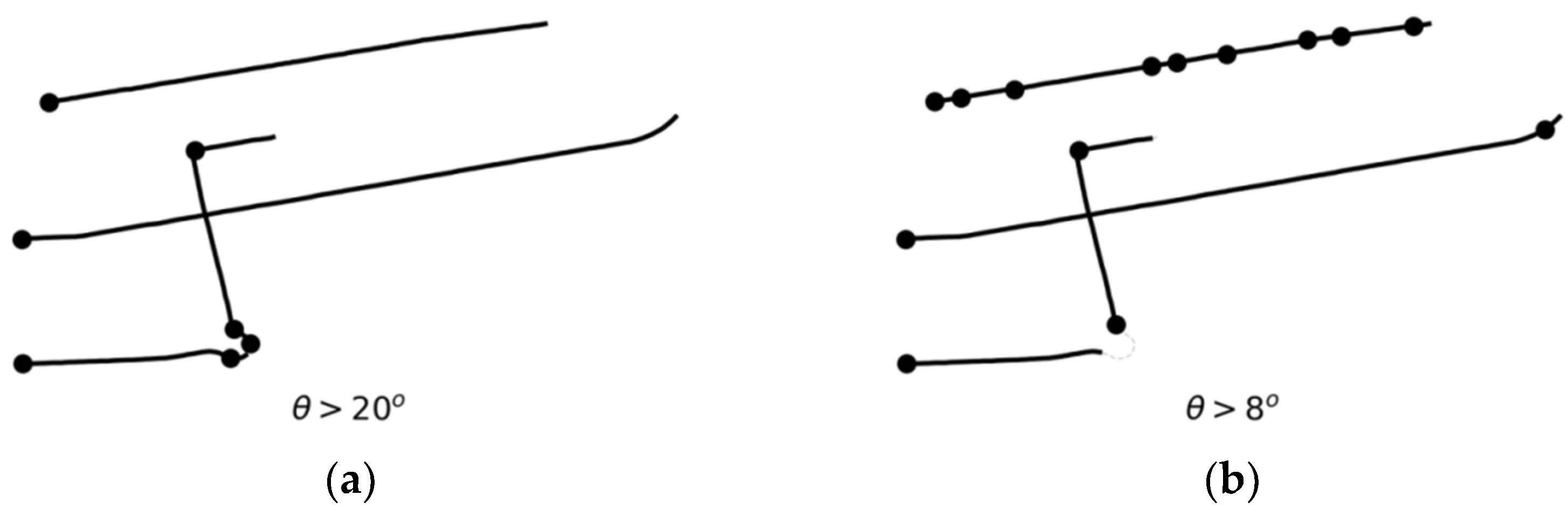
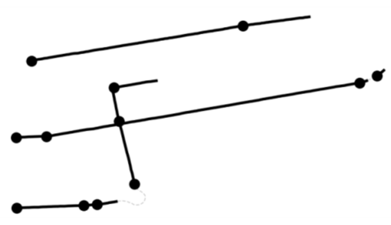
The main basis for identifying intersections in this paper is the fact that straight-line trajectory intersection points mostly occur in the road intersection. In order to better calculate straight-line trajectory intersection points, the straight-line segments of trajectories need to be extracted from the continuous trajectory segments. The most straightforward way to separate straight-line segments from continuous trajectories is to divide them according to the steering angle of each sample point and when the steering angle is greater than a preset threshold, the original continuous trajectory is separated by this sample point and the first half of the separated trajectory forms a straight-line segment; however, it is difficult to use this method of separation based on steering angle threshold to determine a suitable global threshold value and the separation result is very sensitive to this steering angle threshold. When the threshold is too large, trajectories with gradual steering cannot be separated effectively and trajectories with gradual steering behavior are treated as straight-line segments. On the other hand, when the threshold is too small, the separated straight-line trajectory segments are too fragmentary and some trajectories with lane-changing behavior are separated into several straight-line segments, thus losing the original trajectory characteristics. As shown in Figure 3, the lines represent the straight-line segments separated by different steering angle thresholds and the dots are the starting points of the straight-line segments.
To address the difficulty of using the steering angle method to determine a reasonable threshold, this paper proposes a method based on the maximum reconstruction error to extract straight-line segments from the trajectory.
The proposed method assumes that the behavior pattern of the trajectory can be approximated by a spline curve. If a trajectory is fitted well by a spline curve, then the spline and the trajectory have the same pattern; therefore, if a trajectory could be fitted well to a straight-line segment, then this trajectory can be regarded as straight.
The original continuous trajectory is reconstructed as a straight line and the reconstruction errors for whole sampling points are calculated. When the maximum reconstruction error is low enough, the trajectory could be regarded as straight-line.
Let the continuous trajectory with m sampling points be and perform a linear segment reconstruction for TS at the first and last sampling point. The equation of the approximated linear segment about the i-th sampled point after the reconstruction can then be written as
where denotes the position of the i-th sampling point, is the mapping value of the i-th trajectory point in the reconstructed straight-line segment, and is the ratio of the length of the trajectory from the starting sampling point to the i-th sampling points of the total length of the trajectory and has , denoted as
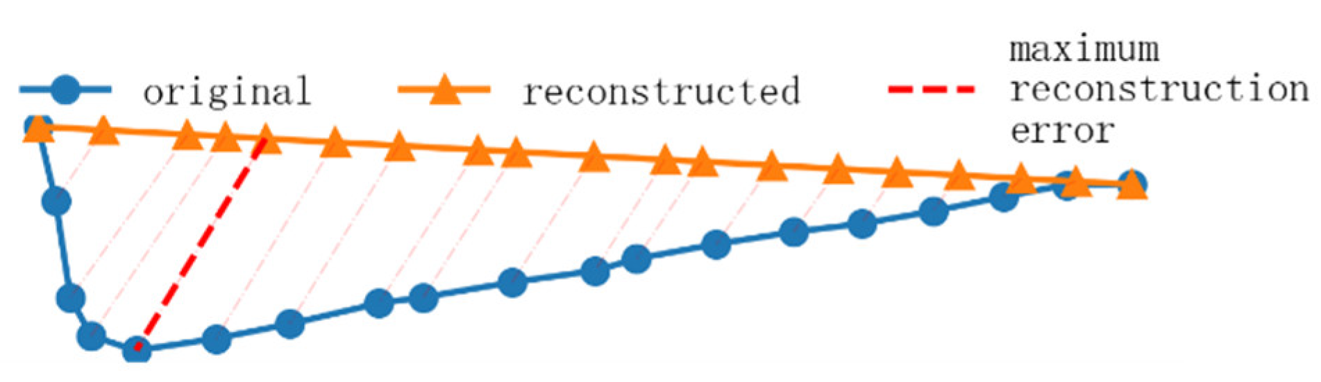
The reconstruction error for a sampling point is the distance between the position in a continuous trajectory and the reconstructed straight-line segment. The reconstruction error for the i-th sampling point is calculated as follows:
The maximum reconstruction error is the maximum value of each reconstruction error and is the position of the maximum reconstruction error value that first occurs from the start of the trajectory. Algorithm 1 is the calculation process of maximum reconstruction error.
| Algorithm 1 Calculate maximum reconstruction error |
| Input: Trajectory sequence Output: , 1. Calculate local distance sequence , where . 2. Calculate cumulative distance sequence , where . 3. Calculate ratio parameter sequence , where . 4. Calculate reconstruction sequence , where . 5. Calculate reconstruction error sequence , where . 6. . 7. For i = 2 to n 8. If : 9. return , . |
The reconstruction error is shown as a dashed line in Figure 4.
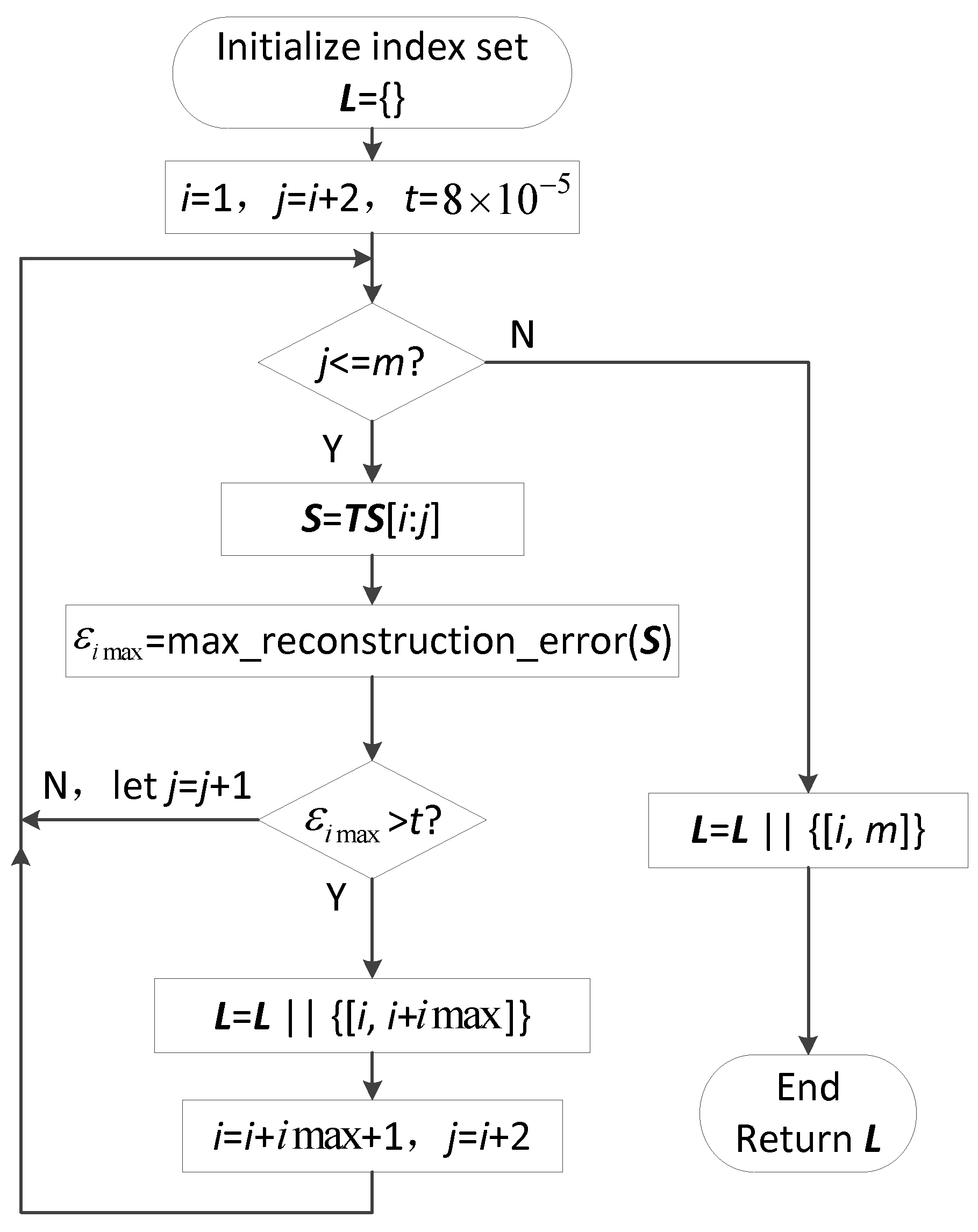
Based on the maximum reconstruction error, the process for separating straight-line segments of a continuous trajectory TS with m sampling points is as Figure 5.
L is used to store the index results of the start and end points of each straight-line segment after separation and S is the sub-trajectory of the continuous trajectory TS. When calculating the maximum reconstruction error for a sub-trajectory S, the index of the maximum reconstruction error in S, denoted as , is also obtained. t is the separation threshold; when the maximum reconstruction error is greater than this threshold, the trajectory is separated by the location of the maximum reconstruction error. The separation threshold t indicates the distance between two locations expressed by latitude and longitude in the mid-latitude (30 to 60 Degrees) range, with the default value indicating approximately 10 m. Algorithm 2 is the process of separating straight-line segment.
| Algorithm 2 Separating straight-line segment |
| Input: Trajectory sequence , threshold Output: Line segment index SegIdxs = 1. Initialize SegIdxs = [] and i = 1. 2. While True: 3. For j = i + 2 to n: 4. , = Algorithm_1 () 5. If : 6. SegIdxs.append() 7. 8. Break for 9. If j > = n: break while 10. SegIdxs.append([i,m]) 11. Return SegIdxs |
The straight-line segment results of separating trajectories using the reconstruction error method are shown in Figure 6, where the lines represent the separated straight-line segments and the dots are the start points of the line segments.
As can be seen from Figure 6, the maximum reconstruction error method is able to separate progressive steering trajectories well and is unaffected by driving behavior, such as lane changes in straight-line trajectories. After straight-line segment extraction, each straight-line trajectory segment is denoted by the position of the start and end points.
2.3. Intersection Points Calculation
There is a large number of similar patterns in the straight-line segments of the trajectory obtained based on the maximum reconstruction error method. To speed up the intersection point calculation process and enhance the road network pattern, this paper first merges the straight-line segments with similar patterns. Then, the pairs of segments that do not have the possibility of intersection points are excluded using bounding box filtering and orthogonal filtering. Finally, the intersection points are calculated in the filtered set of straight-line segments.
2.3.1. Straight-Line Segment Merging
After all continuous trajectories have been separated, there is a large number of similar patterns in the line segments, leading to a large redundancy in calculating the intersection point of line segments. By combining these straight-line segments, not only can the number of straight-line segments to be calculated be effectively reduced, but the combined straight-line segments can better reflect the structure of the road network; therefore, before calculating the intersection point of straight-line segments, we first merge the separated straight-line segments.
The basis for the merging of each straight-line segment is the overlapping straight-line segments that have the same direction and are on the same line; therefore, the specific steps for the merging of straight-line segments consist of three parts: classifying the straight-line segment to the same direction, clustering the co-linear straight-line segment and merging overlapped segments in the same straight line.
- (1)
- Classify straight-line segment in the same direction
In this paper, a hard separation is used to divide the two-dimensional plane into 360-directional clusters and each straight-line segment trajectory is divided into a certain directional cluster. The specific process is to use the unit vector of the vector formed by the position of the start and end points of each straight-line trajectory segment as the direction vector of that straight-line segment trajectory. The cluster unit vector corresponding to each angle in the 360 degrees from 0 to 359 degrees is calculated as the unit direction of each directional cluster. The cluster unit vector is defined as .
To classify the directional clusters of a linear segment trajectory, the inner product of the unit direction vector of the linear segment trajectory to the unit vector of each directional cluster is calculated and then the linear segment trajectory is divided into the directions corresponding to the maximum of the inner product. Let the unit direction of a straight-line segment trajectory be ; the cluster of directions corresponding to deg that maximize is then the cluster of directions in which this straight-line segment trajectory lies.
- (2)
- Clustering of the co-linear straight-line segment
For each directional cluster, the line segments are further divided into co-lines clusters according to distance. A co-line cluster is based on the co-normal distance relationship of the line segments within the same directional cluster and the line segments with a small distance are combined into the same line clusters. In order to automatically determine the amount of co-linear clusters and to avoid truncation caused by hard separation, we used density clustering DBSCAN [23] for co-linear clusters. We set the clustering parameter EPS to and parameter MinPts to 1. The clustering results can well represent the proximity of straight-line segments within a certain co-linear cluster.
- (3)
- Merging overlapped segments in the same straight-line
After Step 2, straight-line segments within the same co-linear cluster are on the same line. These straight-line segments can be merged according to whether there is an overlapped relationship between the intervals of each straight-line segment. To simplify determining the overlap of straight-line segments, all the straight-line segments in a directional cluster are first rotated toward the horizontal direction. Let a be the angle from the positive x-axis to the line segment’s unit direction vector; the unit direction vector can then be written as [cosa, sina]. The rotation transformation matrix is
By performing a rotation transformation with Q for each start and end point of the line segment, the two-dimensional common line segment merging problem is converted to a one-dimensional interval merging problem. The merging process can be completed by traversing all line segments in the collinear cluster once; then, each start and end point of the merged one-dimensional line segment is rotated in QT to transform back to the original two-dimensional space.
2.3.2. Bounding Box and Orthogonal Filtering
This paper calculates the intersection point of any two straight-line segments that have been merged, using the intersection point as the key point in the intersection area; however, there are two problems with calculating the intersection point directly from the merged straight-line segments: (1) there are still too many straight-line segments to calculate the intersection point, resulting in a large amount of computation; (2) the trajectories of the two straight-line segments may have parallel relationships, resulting in a solution that is not unique or does not exist when calculating the intersection point. In order to solve these two problems, we performed two filtering methods on pairs of straight-line segments—bounding box filtering and orthogonality filtering—to remove most of the pairs of straight-line segments without an intersection relationship in advance.
- (1)
- Bounding box filtering. Filter out pairs of straight-line segments for which it is impossible to have an intersection based on two-dimensional spatial relationships. In this paper, an axis-aligned bounding box (AABB) is used for filtering. In two-dimensional space, the axis-aligned bounding box is described aswhere represent, respectively, the minimum longitude, maximum longitude, minimum latitude, and maximum latitude for the start and end points of a line segment. Straight-line segments may intersect only if their bounding boxes intersect; therefore, to determine whether straight-line trajectory segments intersect, first determine whether the bounding box in which each lies intersects. Given two rectangular bounding boxes, RA and RB,
In two dimensions, the condition for the rectangles to intersect must be that they intersect on both of the two axes, as shown in Figure 7.
Therefore, when there is an intersection of two straight-line segments, the rectangular bounding box corresponding to each of the two straight-line segments should satisfy the condition: , , and . We used this condition to quickly filter out a large number of straight-line segments without intersection relationships.
- (2)
- Orthogonality filtering. In this paper, it is assumed that the two straight-line trajectories intersecting at the road intersection are approximately perpendicular to each other, so the angle between the direction vectors of the two straight-line segments can be used to further filter the trajectory segments. When the absolute value of the inner product of the unit direction vectors of the two straight-line segments is greater than the orthogonality threshold (0.5), the angle between the two straight-line segments is small (less than 60 degrees) and the intersection calculation of the trajectories of these two straight-line segments can be filtered out directly. The orthogonality filtering not only further reduces the computation of the intersection point of straight-line segments, but also removes straight-line segments that have parallel relationships, thus ensuring the existence and uniqueness of the solution when computing the intersection of straight-line segments.
2.3.3. Calculating Intersection Points
The intersection point calculation of straight-line segments can be translated into the calculation of the intersection of lines. Let the start and end points of two straight-line segments in the two-dimensional plane be and , respectively. Two real scalar parameters, u and v, satisfy and . Then, the position points and on the two straight-line segments can be expressed in terms of the parametric equations for u and v, respectively.
The intersection of straight lines must satisfy , which can be achieved by solving the linear equation directly:
The solution is obtained for the values of u and v for the parameter corresponding to the intersection of the lines. The existence and uniqueness of the solution is guaranteed because it is filtered for orthogonality. The intersection point of the line segments exists when the parameter values satisfy and the intersection point is .
2.4. Road Intersection Extraction
The intersection points of straight-line segments already reflect the spatial location of the road intersections well, but there is a large number of duplicate intersections; therefore, it is necessary to further cluster the intersections of the straight-line segments. We used a density peaking algorithm to cluster the intersection points and the final road intersection locations were identified by the center of each cluster.
For density peak clustering, where the number of class clusters can be determined automatically, the key hyper-parameter is the cutoff distance used to calculate the local density of each sample. In this paper, the cutoff distance was determined to be 5e-4 based on the Euclidean distance distribution of the latitude and longitude between the intersection points of each straight-line segment. On the other hand, the cutoff distance set in this method is somewhat general, as it has a practical physical meaning, i.e., it represents the smallest possible distance between the two intersections, which is about 60 m.
A Gaussian kernel function was used in the calculation of the local density for each sample. The standard deviation bandwidth of the Gaussian kernel was set to , which is approximately one-third of the cutoff distance, based on the assumption of a normal distribution.
When filtering the decision diagram, in some low-flow or poorly sampled road intersections, there will be few trajectory intersection points, i.e., very little local density and these road intersections will be missed. Therefore, in this paper, local density is not filtered. Global threshold filtering is used for the minimum distance only and the threshold is the cutoff distance. The overall clustering process is described as follows.
In Algorithm 3, first calculate the distance matrix between each line intersection point. Second, calculate the local density of each intersection point based on the cutoff distance and a Gaussian kernel.
| Algorithm 3 Line segment intersection points DPCA |
| Input: Line intersection points matrix , where . Cutoff distance threshold . Gaussian kernel bandwidth . Output: Road Intersection set C |
|
Then, calculate the index sequence which is sorted by local density. Our density peak clustering implementation proposes this sorted index; it avoids the problem caused by the same local density when calculating the minimum distance and improves the calculation efficiency.
Furthermore, calculate the minimum distance from each intersection point to any other higher-density intersection point. Finally, select the sample with the minimum distance greater than the cutoff distance as the center of each road intersection.
Since only the minimum distance needs to be filtered when determining the cluster centers, it is more concise compared to the traditional density peaking algorithm.
3. Experiment
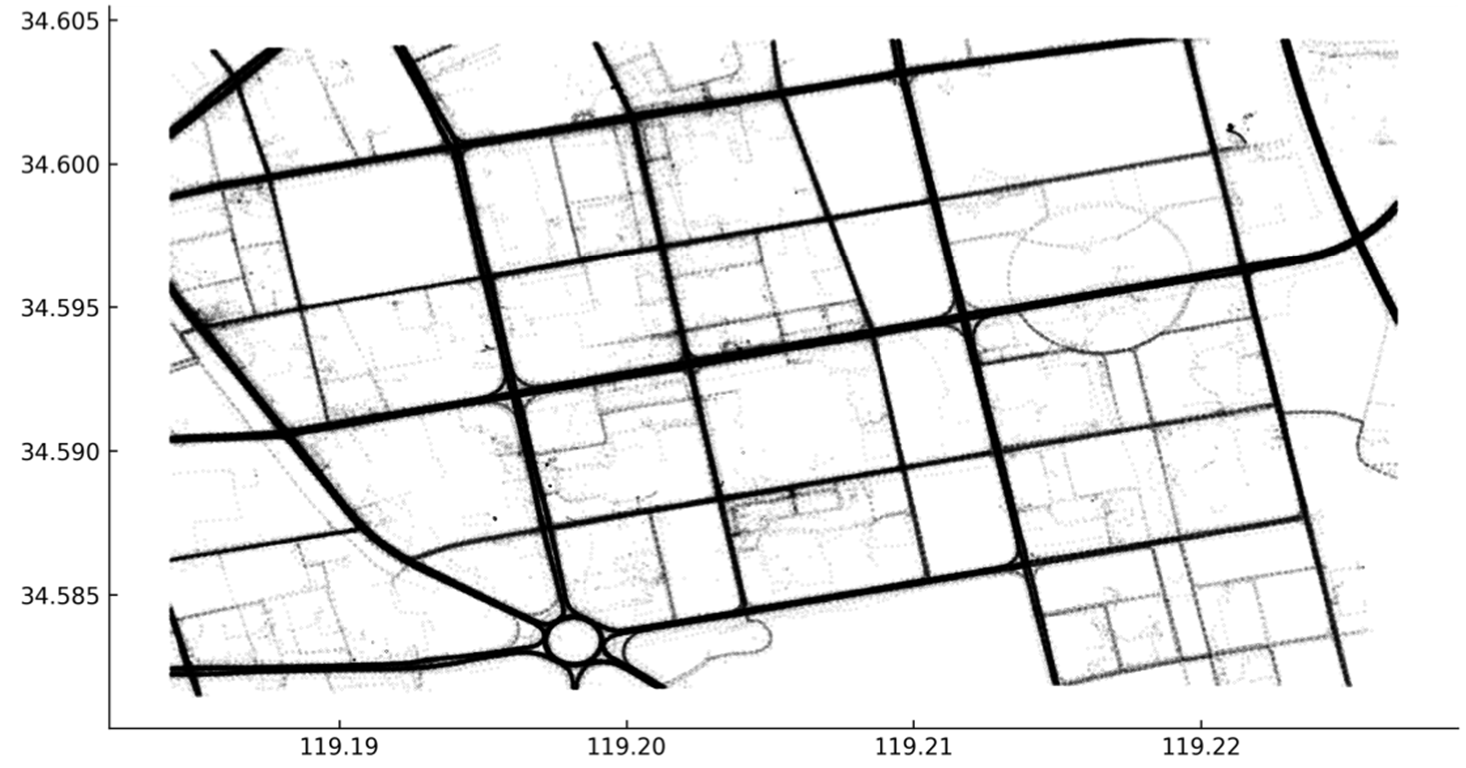
To validate the method in this paper, the road intersections in an area were automatically extracted. The trajectory dataset was from Baidu Map navigation data for the Haizhou district of Lianyungang City in China. The data time covered the whole day of 1 January 2019; this dataset contained a total of about 5 × 10⁵ sampling points and about 5 × 10³ raw trajectories, and contained fields for vehicle identification, sampling time, longitude and latitude. The spatial distribution of all sampling points is shown in Figure 8.
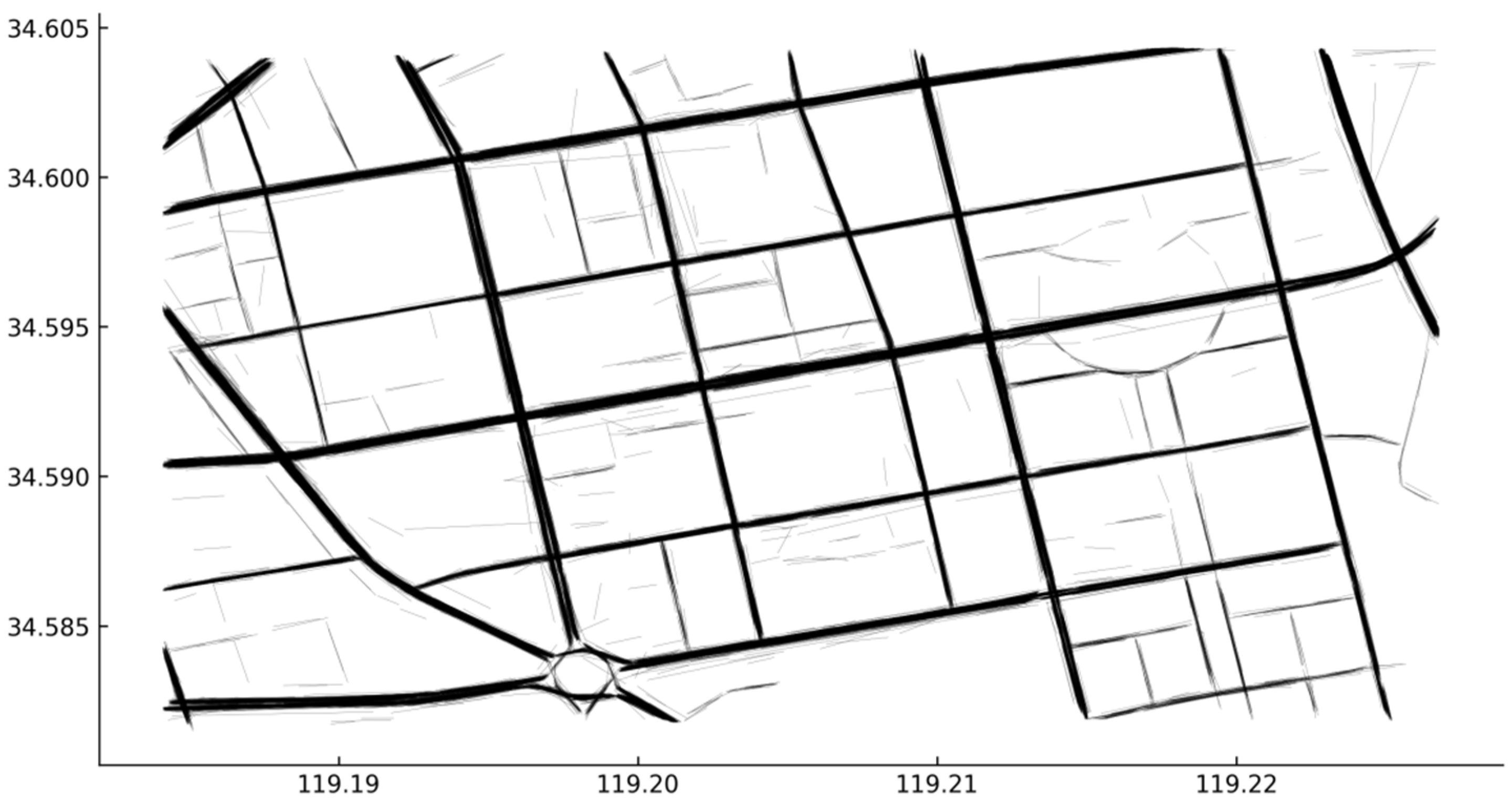
From the original trajectory dataset, 53,960 continuous trajectories were extracted, of which 25,373 were valid continuous trajectories. The maximum reconstruction error method was used to extract 28,399 straight-line segments from the valid continuous trajectory. These extracted straight-line segments are shown in Figure 9.
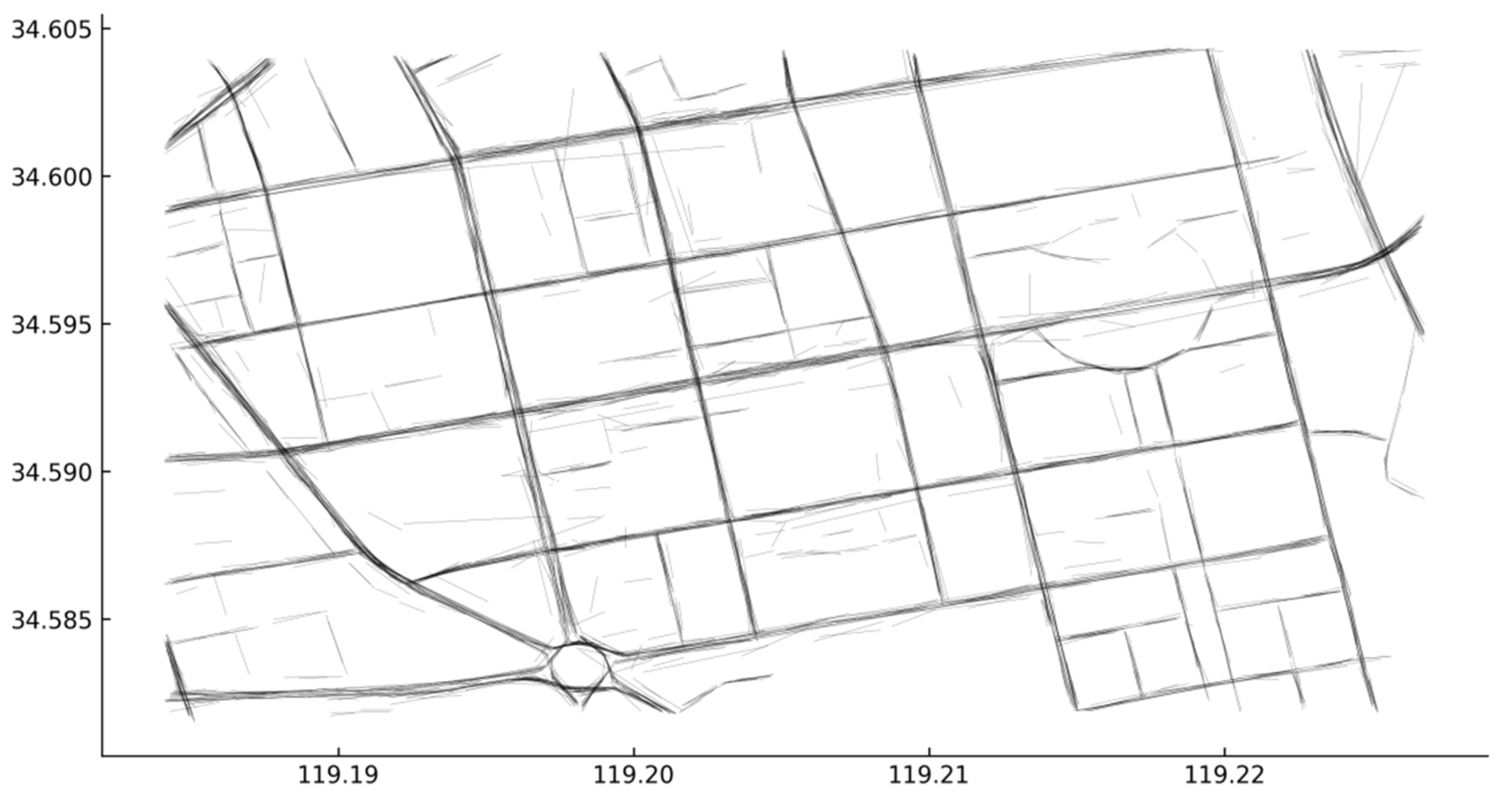
The merged straight-line segments amount was 2502, only about 10% of the total amount of extracted straight-line segments; it not only reduced the amount of data to be calculated for the intersections, but also enhanced the structure of the road network represented by the individual line segments. These merged line segments are shown in Figure 10.
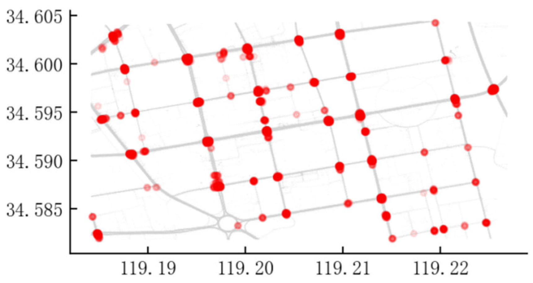
When calculating the intersection points using the merged trajectories, we removed the short trajectories and the actual number of line segments involved in the intersection point calculation was 1243. The intersection of any two straight lines requires 1243 × (1243−1)/2 (about 7.7 × 10⁵) intersections. Through the bounding box filter and orthogonality filter, the intersection point calculation is reduced by 96.3%, requiring only 2.8 × 10⁴ calculations (of which the bounding box filter reduced the calculation by about 90% and the orthogonality filter reduced the calculation by about 6%). As the complexity of the filtering calculation is much less than that of the intersection calculation of straight-line segments and as multiple lines can be filtered simultaneously by vector operations, the total calculation time was reduced by 94.3%, which significantly improved the efficiency of the calculation. The final number of intersection points was 4273 and the spatial distribution of all intersection points are shown in Figure 11 as red dots.
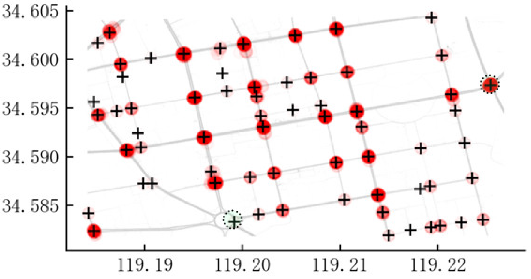
Finally, after clustering the calculated intersection points by spatial location, adaptive thresholding was used for intersection extraction and 65 intersections were extracted, with the results shown in Figure 12. The black crosses are extracted road intersections.
Compared with intersection extraction methods based on features such as trajectory steering angles and stopping points, the method in this paper is less affected by trajectory sampling amount; it can identify intersections with lower sampling amounts and, at the same time, be well suited to the situation where the density of trajectories is unevenly distributed in a wide range of road networks.
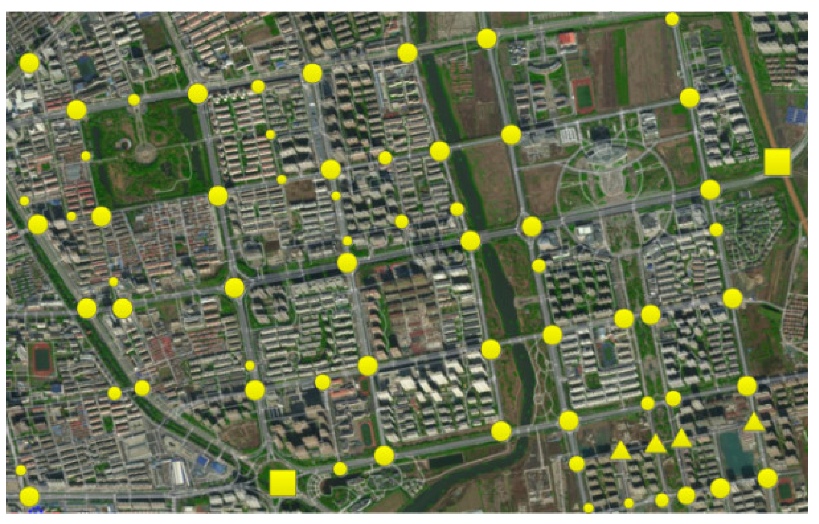
The real locations and number of intersections in the study area are shown in Figure 13, where the dots are the intersections successfully identified in this paper, but there were still some road intersections that were not identified (triangles) for the following reason: the road intersections were T-junctions and straight-line trajectories did not have direct intersection points. The square locations in the figure are the roundabouts and overpasses, respectively, which were misidentified as intersections, corresponding to the circular dashed boxed area in Figure 12.
To further validate the method in this paper, the density peak clustering method based on vehicle turning point features proposed by GAO [11] was compared with the global threshold (DPCA).
As can be seen from Table 1, the recognition accuracy of the method in this paper is better than the benchmark method.
4. Conclusions
In this paper, the geometric structure of trajectories is used to achieve the automatic extraction of urban road intersections using extract straight-line segments and calculating their intersection points. The main conclusions obtained are as follows.
- (1)
- Compared with research methods in intersection extraction that use the vehicle steering angle and stopping point as trajectory features, this paper uses trajectory line segment intersection points for intersection extraction, which are less affected by the distribution of sampling data amount, and which can effectively identify intersections in low-traffic or low-sampling areas.
- (2)
- A maximum reconstruction error method is proposed to extract straight-line segments, which can effectively avoid the problem that the threshold value of the steering angle is difficult to determine and can effectively segment the progressive steering trajectory, while at the same time eliminating the fluctuations in the trajectory caused by lane changing and drift.
- (3)
- By merging straight-line segments, the road network structure pattern represented by straight-line segment trajectories is effectively enhanced, the confidence of intersection calculation is improved and the number of straight-line segments to be calculated for intersections can be reduced by 90%. The use of orthogonal and bounding box filtering using the spatial relationship of straight-line segments reduced the intersection calculation by 96%.
However, besides cross-type intersections, there are other types of intersections, such as T-intersection, Y-intersection and roundabouts and our approach only identifies intersections with angles formed of legs greater than 60°; therefore, there is a need to further improve our method for identification of intersections of different types. There is another limitation of our approach. We assume that the minimum distance between intersections is about 60 m; therefore, when distances of multiple adjacent intersections are all less than 60 m, only one intersection can be identified. In our approach, the straight-line segments are directly extracted from each single trajectory; therefore, the greater the amount of valid trajectory, the more straight-line segments would be extracted; however, a greater number of straight-line segments would involve unexpected behavior leading to misidentification. Such limitations will be considered in future work.
Author Contributions
Conceptualization, J.L.; Data curation, J.Y.; Investigation, L.W.; Methodology, L.G. All authors have read and agreed to the published version of the manuscript.
Funding
This research was funded by Beijing Social Science Foundation grant number 21XCC013.
Data Availability Statement
The data presented in this study are available on request from the corresponding author.
Conflicts of Interest
The authors declare no conflict of interest.
References
- Dai, J.; Wang, Y.; Li, W.; Zuo, Y. Automatic Method for Extraction of Complex Road Intersection Points From High-Resolution Remote Sensing Images Based on Fuzzy Inference. IEEE Access 2020, 8, 39212–39224. [Google Scholar] [CrossRef]
- Saeedimoghaddam, M.; Stepinski, T.F. Automatic extraction of road intersection points from USGS historical map series using deep convolutional neural networks. Int. J. Geogr. Inf. Sci. 2020, 34, 947–968. [Google Scholar] [CrossRef]
- Mousavizadeh, O.; Keyvan-Ekbatani, M.; Logan, T.M. Real-time turning rate estimation in urban networks using floating car data. Transp. Res. Part C Emerg. Technol. 2021, 133, 103457. [Google Scholar] [CrossRef]
- Sun, S.; Chen, J.; Sun, J. Traffic congestion prediction based on GPS trajectory data. Int. J. Distrib. Sens. Netw. 2019, 15, 155014771984744. [Google Scholar] [CrossRef]
- Tang, J.; Deng, M.; Huang, J.; Liu, H.; Chen, X. An Automatic Method for Detection and Update of Additive Changes in Road Network with GPS Trajectory Data. ISPRS Int. J. Geo-Inf. 2019, 8, 411. [Google Scholar] [CrossRef] [Green Version]
- Wang, H.; Gu, C.; Ochieng, W.Y. Vehicle Trajectory Reconstruction for Signalized Intersections with Low-Frequency Floating Car Data. J. Adv. Transp. 2019, 2019, 9417471. [Google Scholar] [CrossRef]
- Deng, M.; Huang, J.; Zhang, Y.; Liu, H.; Tang, L.; Tang, J.; Yang, X. Generating urban road intersection models from low-frequency GPS trajectory data. Int. J. Geogr. Inf. Sci. 2018, 32, 2337–2361. [Google Scholar] [CrossRef]
- Tang, J.; Deng, M.; Huang, J.; Liu, H. A Novel Method for Road Intersection Construction From Vehicle Trajectory Data. IEEE Access 2019, 7, 95065–95074. [Google Scholar] [CrossRef]
- Wang, J.; Wang, C.; Song, X.; Raghavan, V. Automatic intersection and traffic rule detection by mining motor-vehicle GPS trajectories. Comput. Environ. Urban Syst. 2017, 64, 19–29. [Google Scholar] [CrossRef]
- Hu, R.; Xia, Y.; Hsu, C.-Y.; Chen, H.; Xu, W. Traffic Intersection Detection Using Floating Car Data. In Proceedings of the 2020 5th IEEE International Conference on Big Data Analytics (ICBDA), Xiamen, China, 8–11 May 2020; IEEE: Xiamen, China, 2020; pp. 116–120. [Google Scholar]
- Gao, L.; Wei, L.; Yang, J.; Li, J. Automatic Recognition of Intersections Based on Vehicle Trajectory Turning Points Clustering. In Proceedings of the 2021 IEEE 4th International Conference on Computer and Communication Engineering Technology (CCET), Beijing, China, 13–15 August 2021; pp. 48–52. [Google Scholar]
- Huang, T.; Sharma, A. Intersection Identification Using Large-scale Vehicle Trajectory Data. In Proceedings of the 5th Conference of Transportation Research Group of India, Bhopal, India, 18–21 December 2019. [Google Scholar]
- Chen, B.; Ding, C.; Ren, W.; Xu, G. Extended Classification Course Improves Road Intersection Detection from Low-Frequency GPS Trajectory Data. ISPRS Int. J. Geo-Inf. 2020, 9, 181. [Google Scholar] [CrossRef] [Green Version]
- Zourlidou, S.; Sester, M. Intersection Detection Based on Qualitative Spatial Reasoning on Stopping Point Clusters. ISPRS-Int. Arch. Photogramm. Remote Sens. Spat. Inf. Sci. 2016, XLI-B2, 269–276. [Google Scholar] [CrossRef] [Green Version]
- Zhou, Y.; Fang, Z.; Thill, J.-C.; Li, Q.; Li, Y. Functionally critical locations in an urban transportation network: Identification and space–time analysis using taxi trajectories. Comput. Environ. Urban Syst. 2015, 52, 34–47. [Google Scholar] [CrossRef]
- Wang, C.; Hao, P.; Wu, G.; Qi, X.; Lyu, T.; Barth, M. Intersection and Stop Bar Position Extraction from Crowdsourced GPS Trajectories. In Proceedings of the Transportation Research Board Annual Meeting 2017, Washington, DC, USA, 8–12 January 2017. [Google Scholar]
- Keler, A.; Krisp, J.M.; Ding, L. Detecting vehicle traffic patterns in urban environments using taxi trajectory intersection points. Geo-Spat. Inf. Sci. 2017, 20, 333–344. [Google Scholar] [CrossRef] [Green Version]
- Wang, J.; Rui, X.; Song, X.; Tan, X.; Wang, C.; Raghavan, V. A novel approach for generating routable road maps from vehicle GPS traces. Int. J. Geogr. Inf. Sci. 2015, 29, 69–91. [Google Scholar] [CrossRef]
- Fathi, A.; Krumm, J. Detecting Road Intersections from GPS Traces. In Geographic Information Science; Lecture Notes in Computer Science; Fabrikant, S.I., Reichenbacher, T., van Kreveld, M., Schlieder, C., Eds.; Springer: Berlin/Heidelberg, Germany, 2010; Volume 6292, pp. 56–69. ISBN 978-3-642-15299-3. [Google Scholar]
- Zhao, L.; Mao, J.; Pu, M.; Liu, G.; Jin, C.; Qian, W.; Zhou, A.; Wen, X.; Hu, R.; Chai, H. Automatic Calibration of Road Intersection Topology using Trajectories. In Proceedings of the 2020 IEEE 36th International Conference on Data Engineering (ICDE), Dallas, TX, USA, 20–24 April 2020; IEEE: Dallas, TX, USA, 2020; pp. 1633–1644. [Google Scholar]
- Li, L.; Li, D.; Xing, X.; Yang, F.; Rong, W.; Zhu, H. Extraction of Road Intersections from GPS Traces Based on the Dominant Orientations of Roads. ISPRS Int. J. Geo-Inf. 2017, 6, 403. [Google Scholar] [CrossRef] [Green Version]
- Rodriguez, A.; Laio, A. Clustering by fast search and find of density peaks. Science 2014, 344, 1492–1496. [Google Scholar] [CrossRef] [PubMed] [Green Version]
- Ester, M.; Kriegel, H.-P.; Sander, J.; Xu, X. A Density-Based Algorithm for Discovering Clusters in Large Spatial Databases with Noise. In Proceedings of the 2nd International Conference on Knowledge Discovery and Data Mining (KDD-96), Portland, OR, USA, 2–4 August 1996; p. 6. [Google Scholar]
Figure 1.
The workflow for extracting road intersections.

Figure 2.
Distribution of the sampling interval of the original trajectory.

Figure 3.
(a) Straight segment (steering angle threshold > 20); (b) Straight segment (steering angle threshold > 8).
Figure 3.
(a) Straight segment (steering angle threshold > 20); (b) Straight segment (steering angle threshold > 8).

Figure 4.
Maximum reconstruction error.

Figure 5.
Flow diagram of straight-line segmentation.

Figure 6.
Straight-line segment extraction using the maximum reconstruction error method.

Figure 7.
Example of AABB overlapping.

Figure 8.
Scatter of original GPS data.

Figure 9.
Extracted straight-line segments.

Figure 10.
Merged straight-line segments.

Figure 11.
Scatter of intersection points.

Figure 12.
Results of intersection extraction (65).

Figure 13.
Location of real intersections in the area of the dataset.


Table 1.
Comparison of intersection extraction methods.
| Method | Extraction Total | Number of Misidentifications |
|---|---|---|
| Steering angle feature | 61 | 7 |
| This paper | 65 | 2 |
Publisher’s Note: MDPI stays neutral with regard to jurisdictional claims in published maps and institutional affiliations. |
© 2022 by the authors. Licensee MDPI, Basel, Switzerland. This article is an open access article distributed under the terms and conditions of the Creative Commons Attribution (CC BY) license (https://creativecommons.org/licenses/by/4.0/).
Share and Cite
MDPI and ACS Style
Gao, L.; Wei, L.; Yang, J.; Li, J. Automatic Intersection Extraction Method for Urban Road Networks Based on Trajectory Intersection Points. Appl. Sci. 2022, 12, 5873. https://0-doi-org.brum.beds.ac.uk/10.3390/app12125873
AMA Style
Gao L, Wei L, Yang J, Li J. Automatic Intersection Extraction Method for Urban Road Networks Based on Trajectory Intersection Points. Applied Sciences. 2022; 12(12):5873. https://0-doi-org.brum.beds.ac.uk/10.3390/app12125873
Chicago/Turabian StyleGao, Lei, Lu Wei, Jian Yang, and Jinhong Li. 2022. "Automatic Intersection Extraction Method for Urban Road Networks Based on Trajectory Intersection Points" Applied Sciences 12, no. 12: 5873. https://0-doi-org.brum.beds.ac.uk/10.3390/app12125873
Note that from the first issue of 2016, this journal uses article numbers instead of page numbers. See further details here.