
On the Resonant Vibrations Control of the Nonlinear Rotor Active Magnetic Bearing Systems

 ,
,  and
and 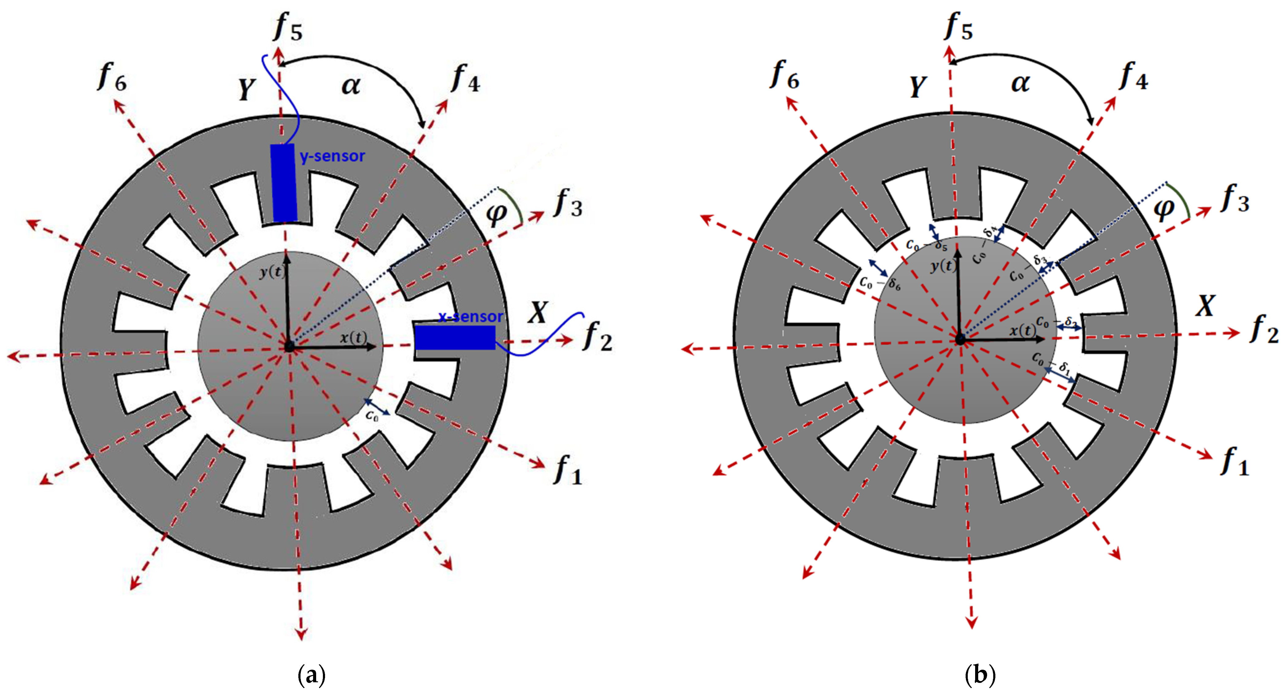
Abstract
:1. Introduction
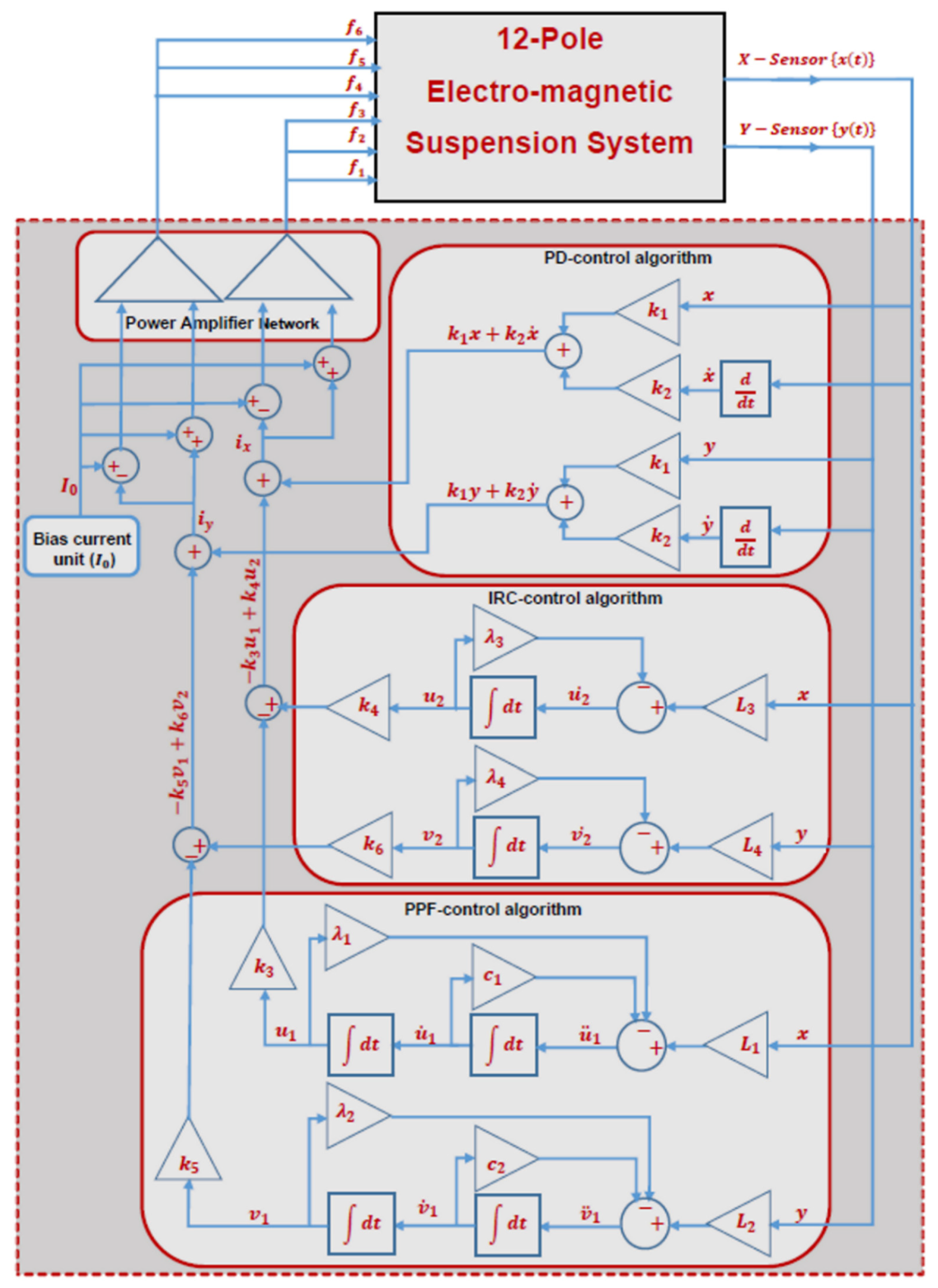
2. Equations of Motion
3. Analytical Investigations
4. Steady-State Oscillation and Bifurcation Analysis
4.1. System Dynamics in the Case of -Control Algorithm
4.2. System Dynamics in the Case of the -Control Algorithm
4.3. System Dynamics in the Case of the -Control Algorithm
4.4. System Dynamics in the Case of -Control Algorithm
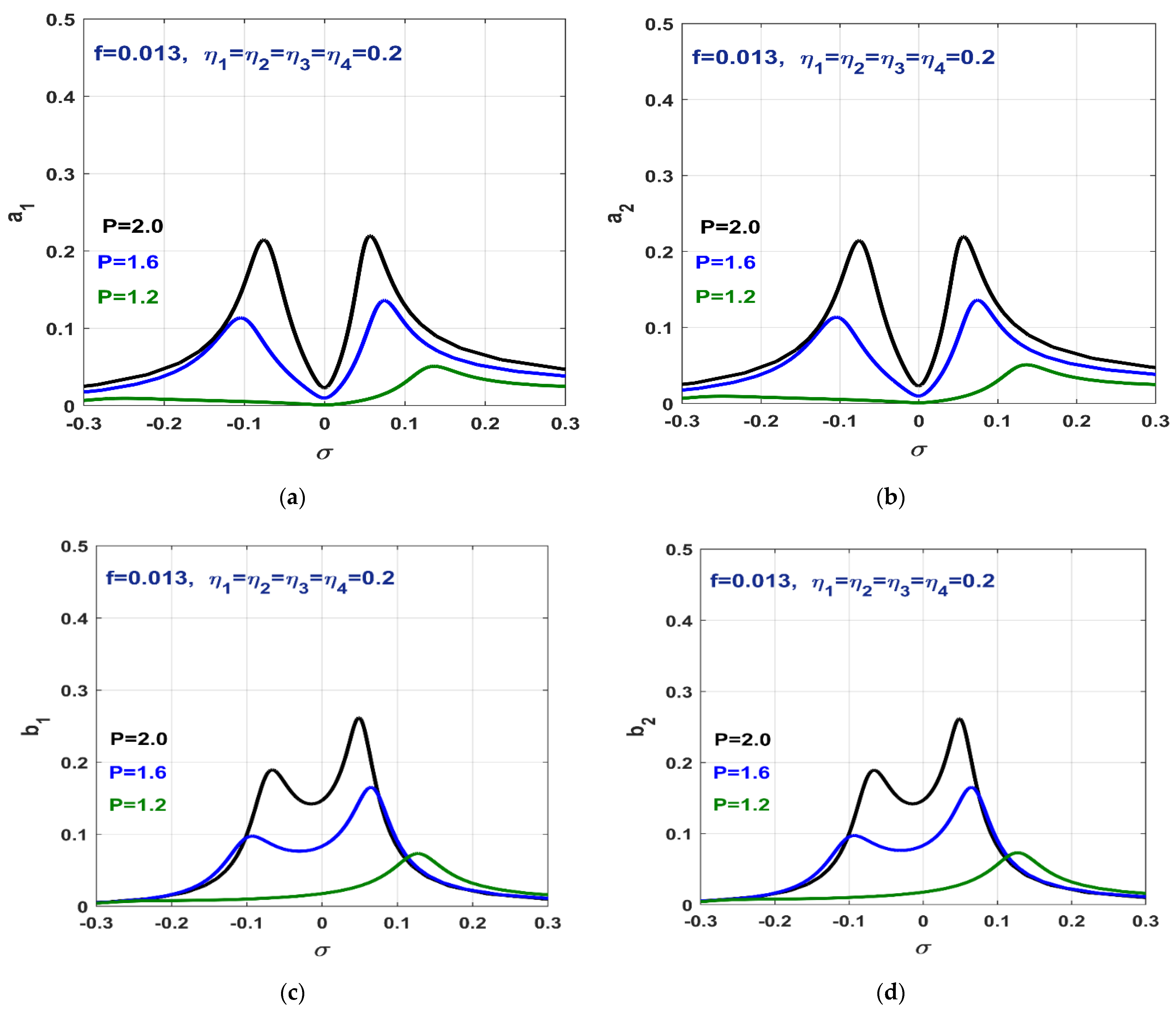
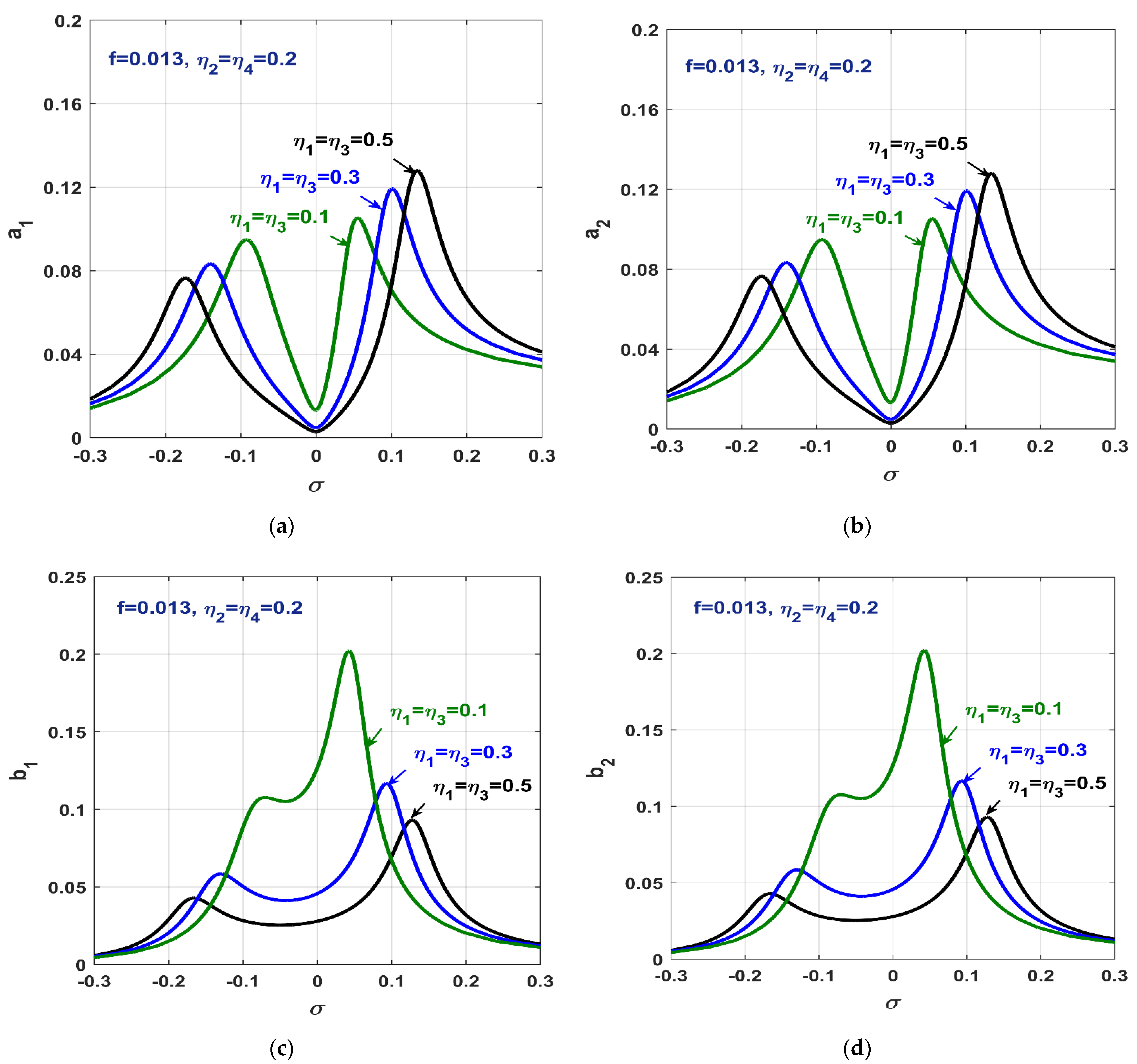
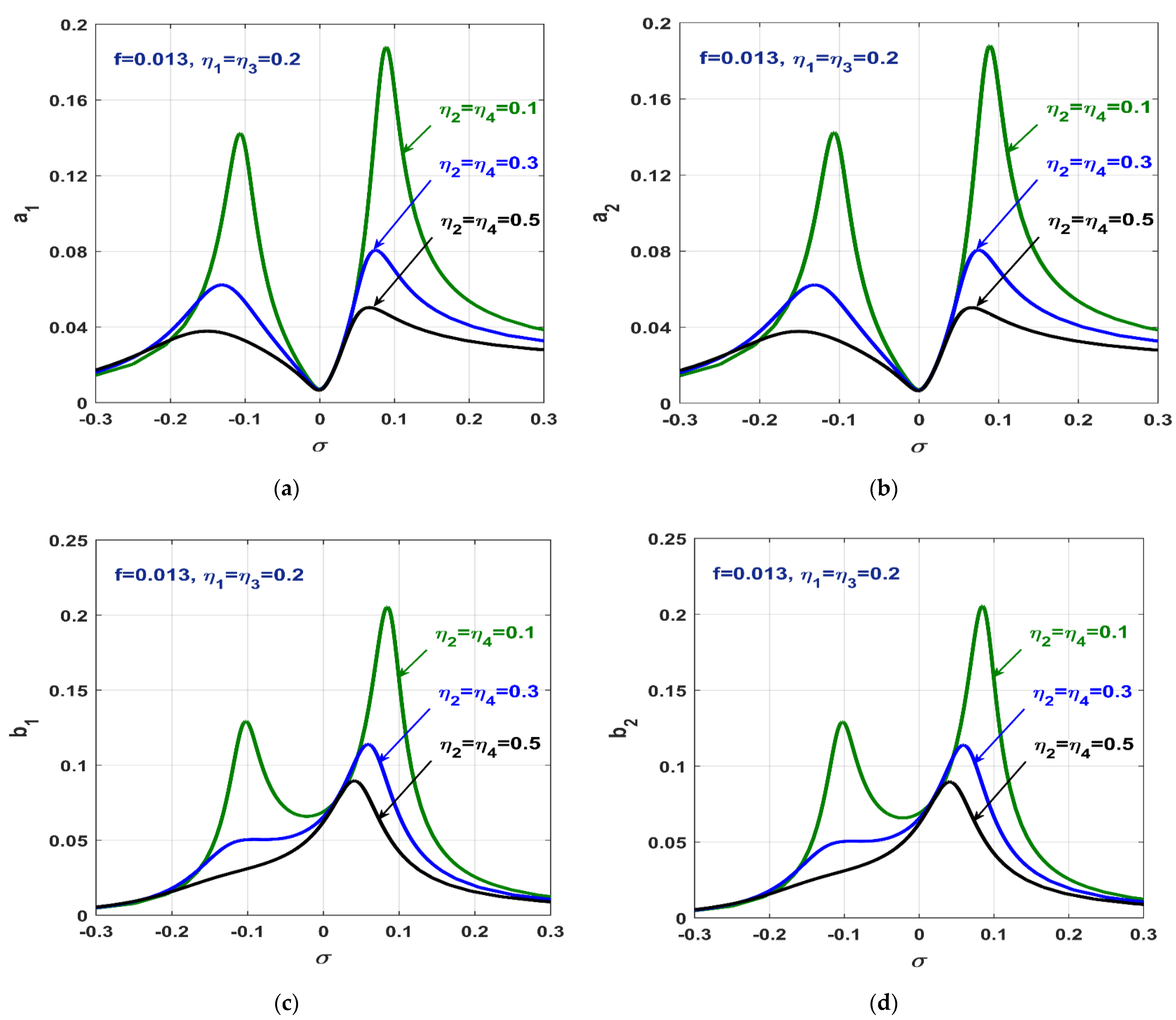
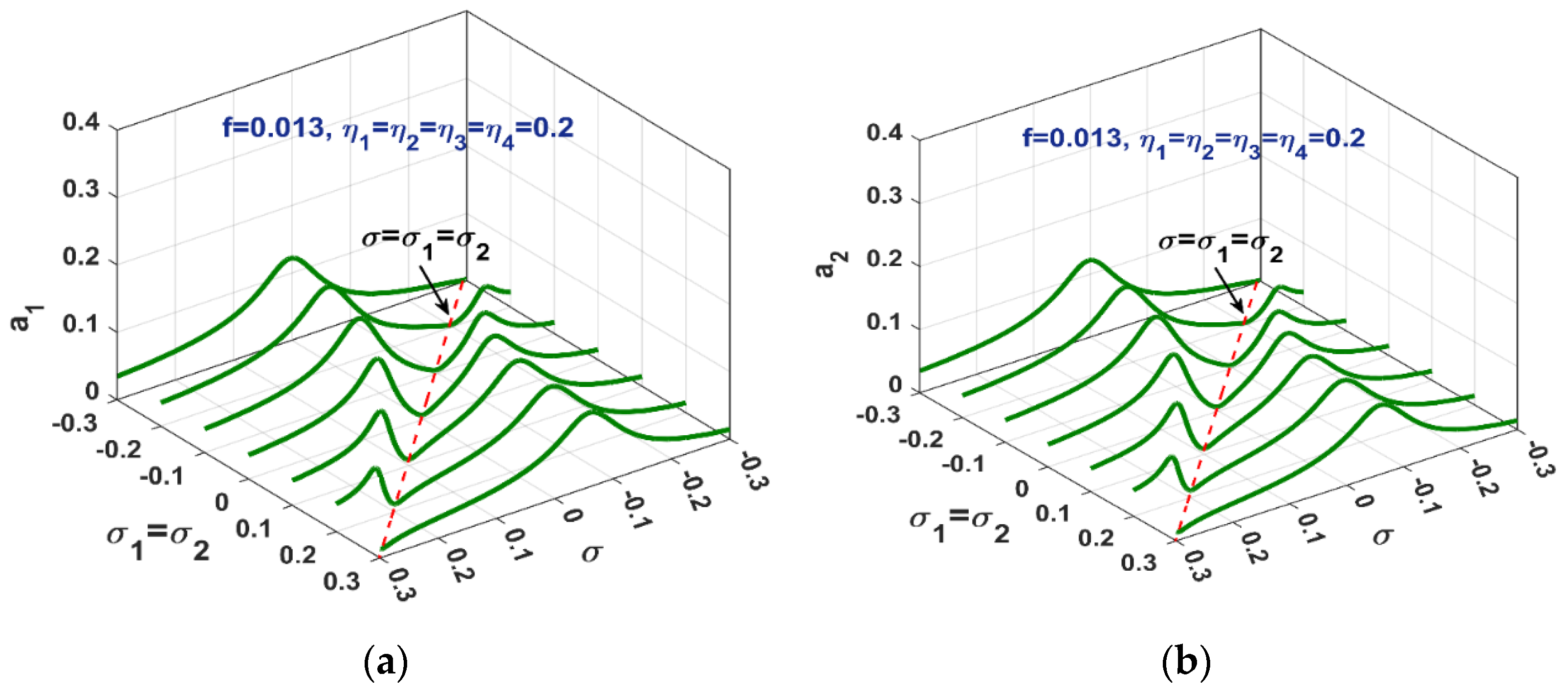
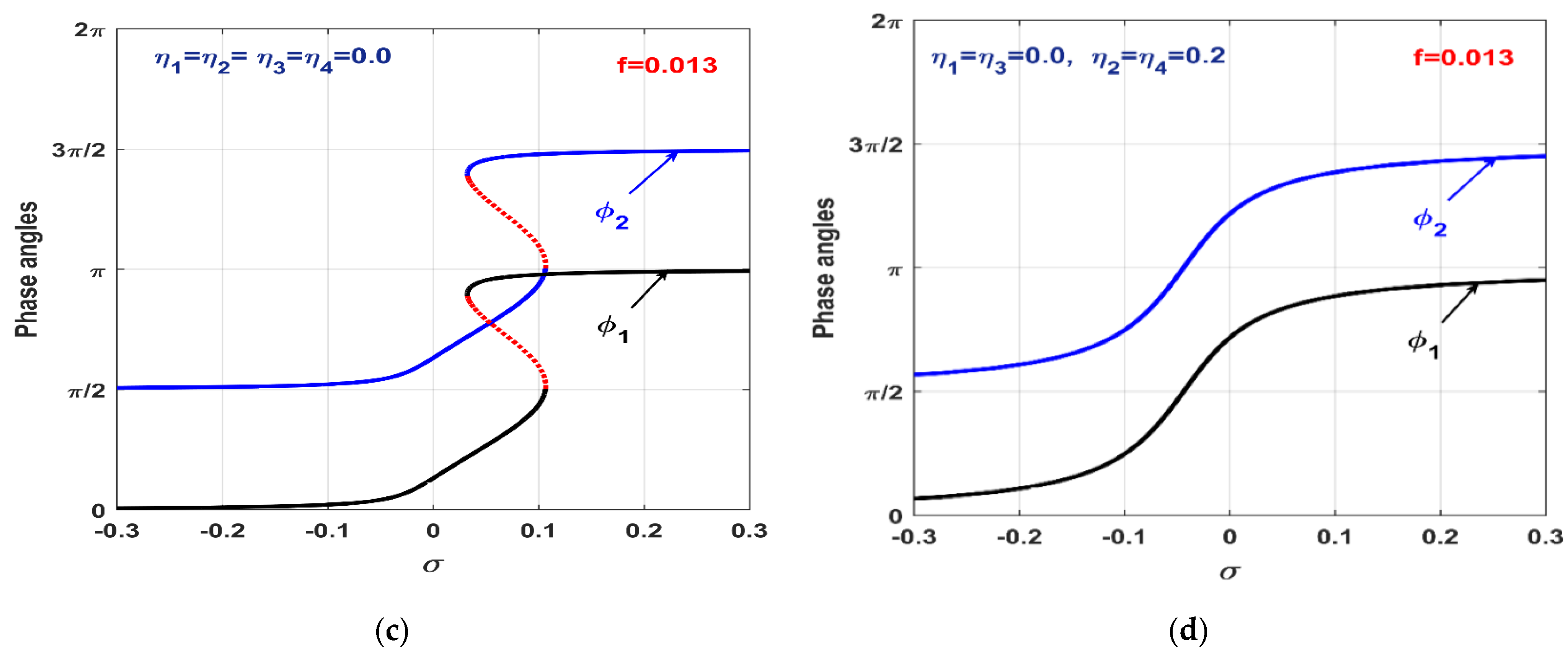
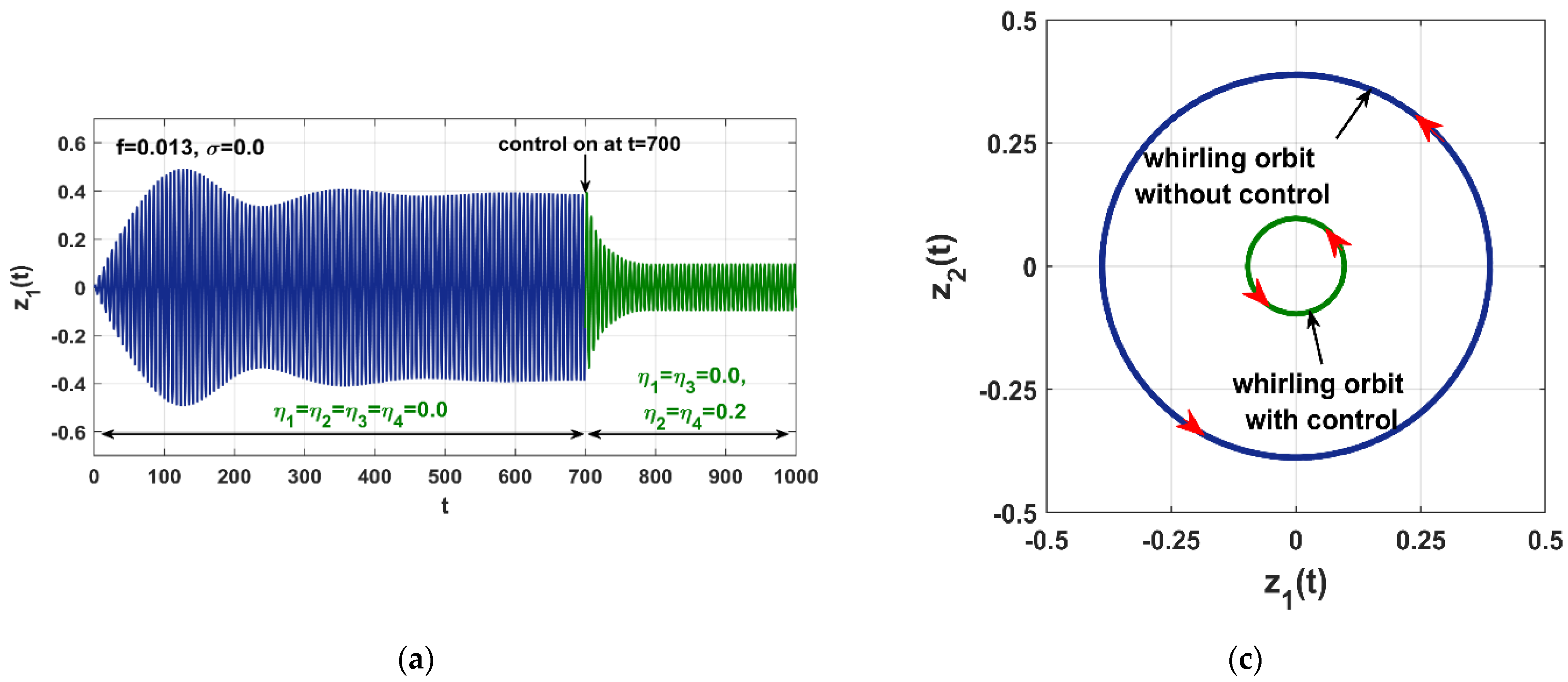
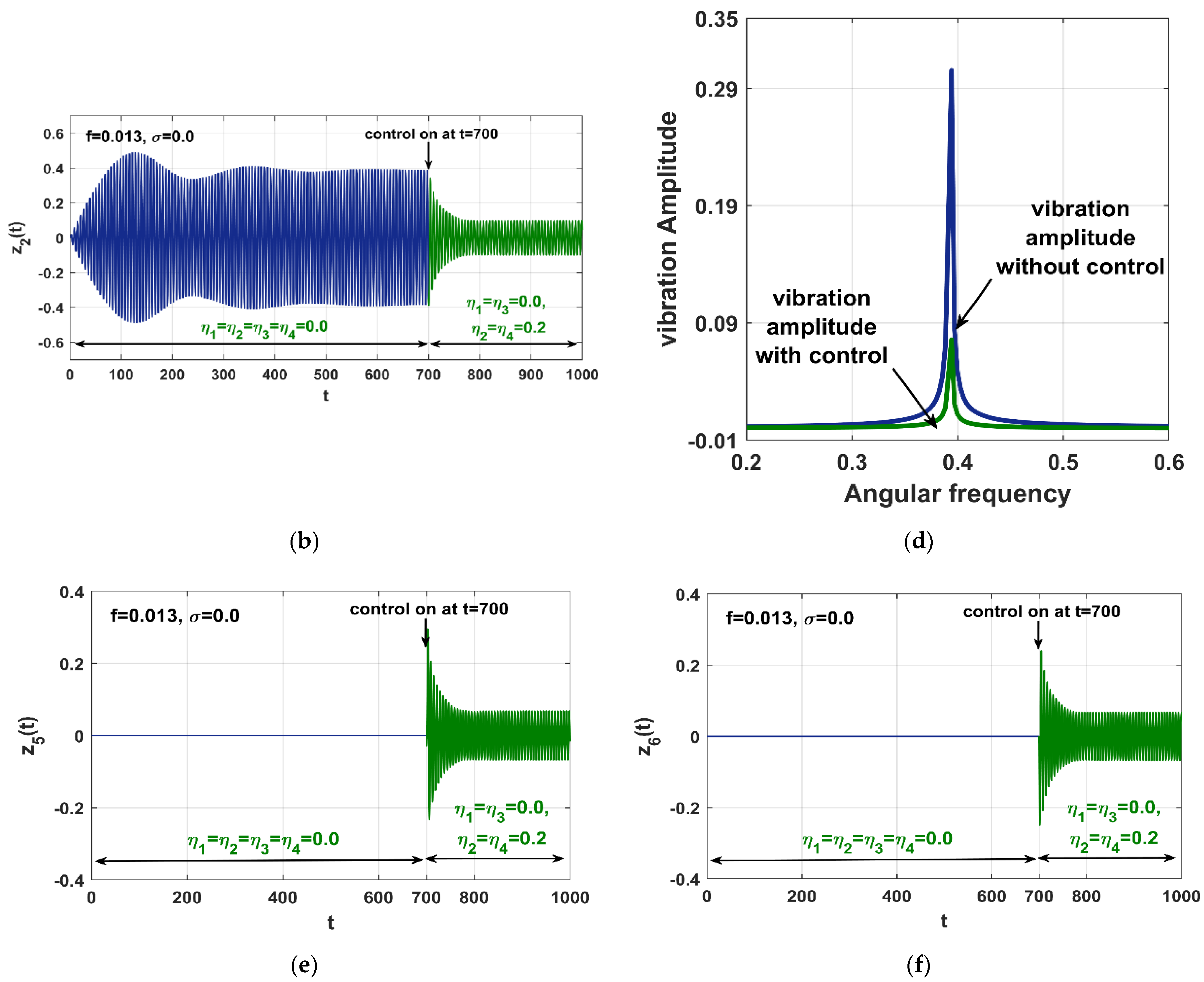
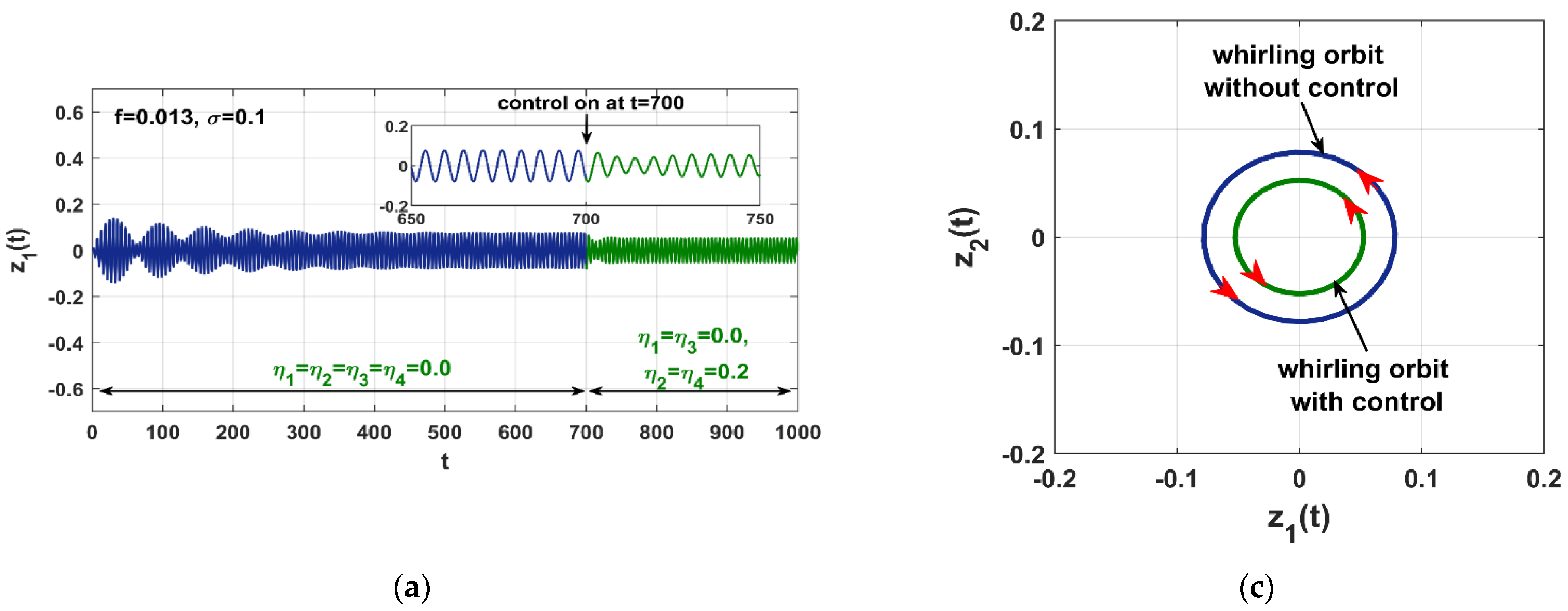
4.5. Sensitivity Analysis of the -Control Algorithm
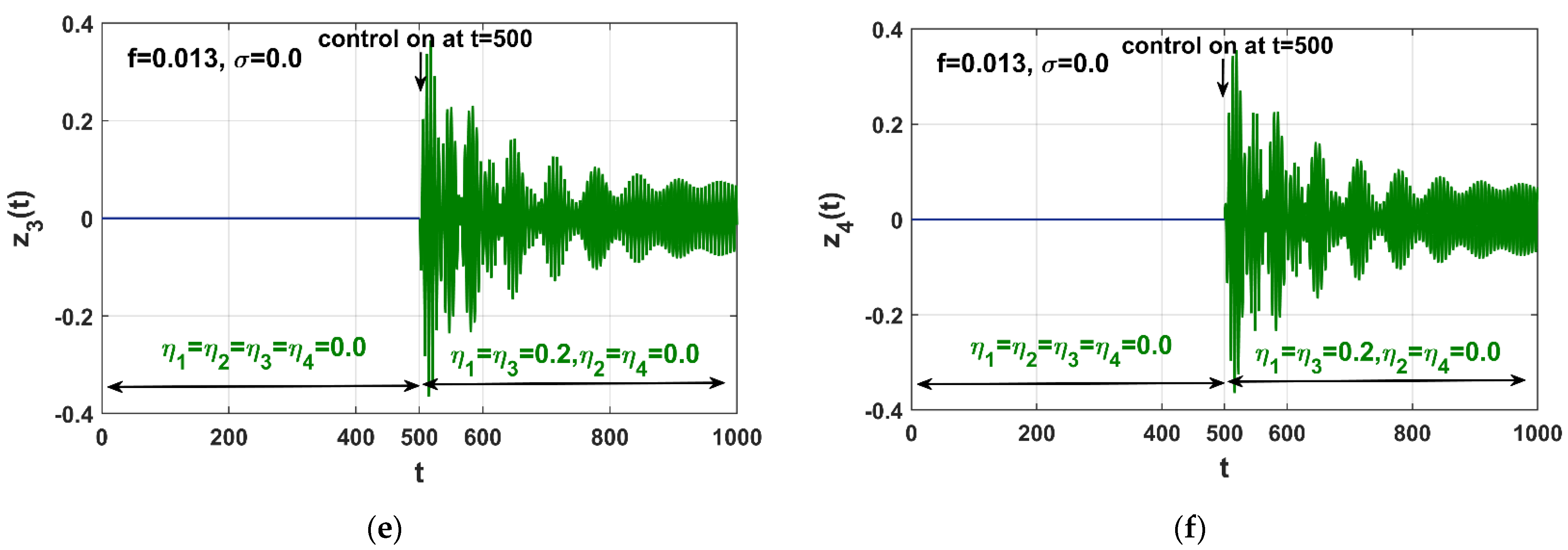
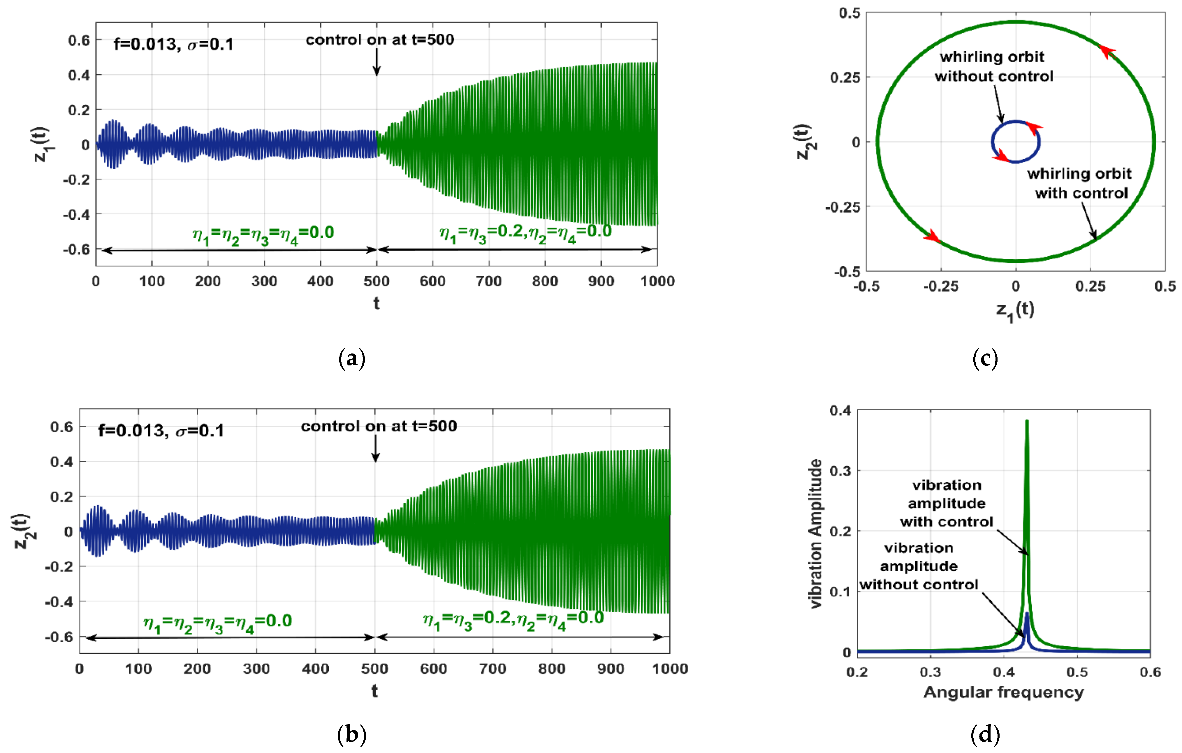
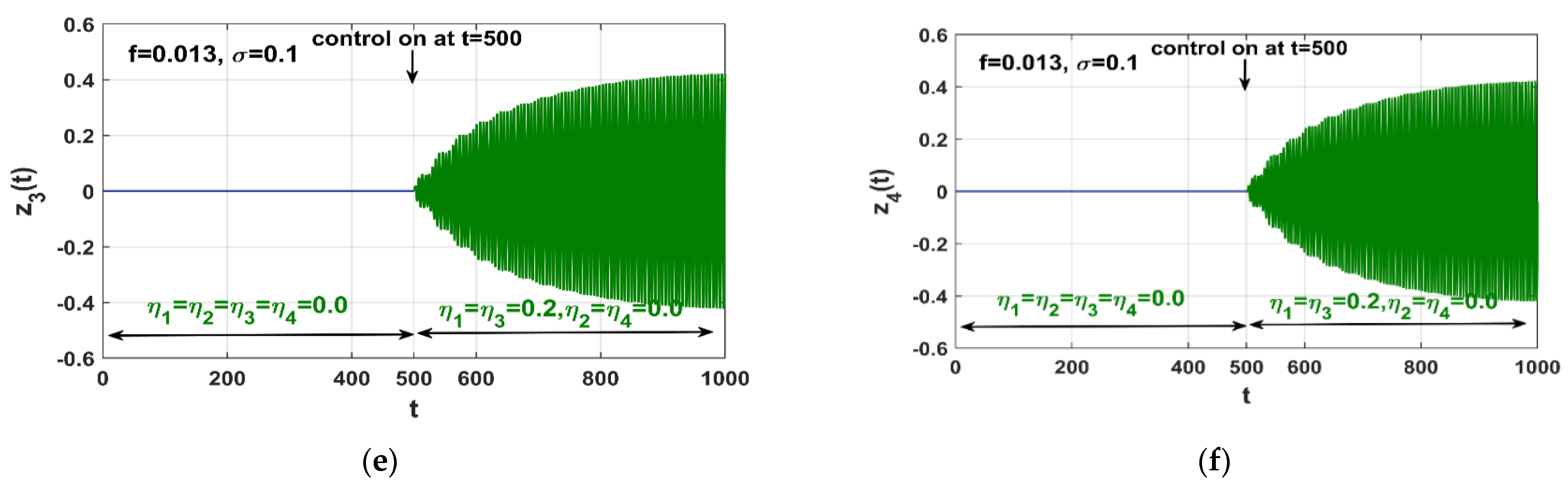
5. Numerical Simulations and Comparative Study
6. Conclusions
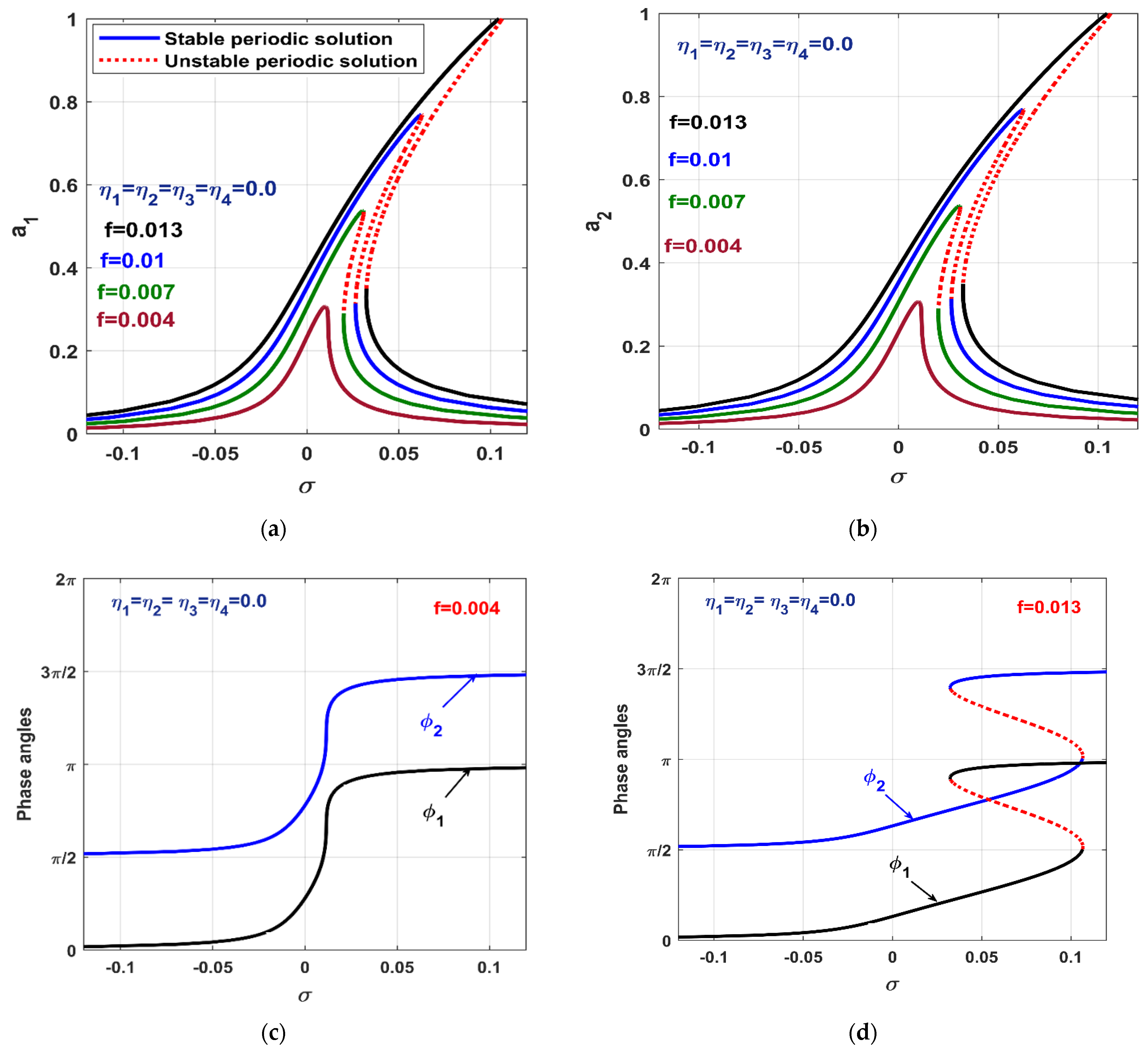
- The rotor system responds as a linear dynamical system with small vibration amplitudes in the case of the PD-control algorithm, as long as the excitation force .
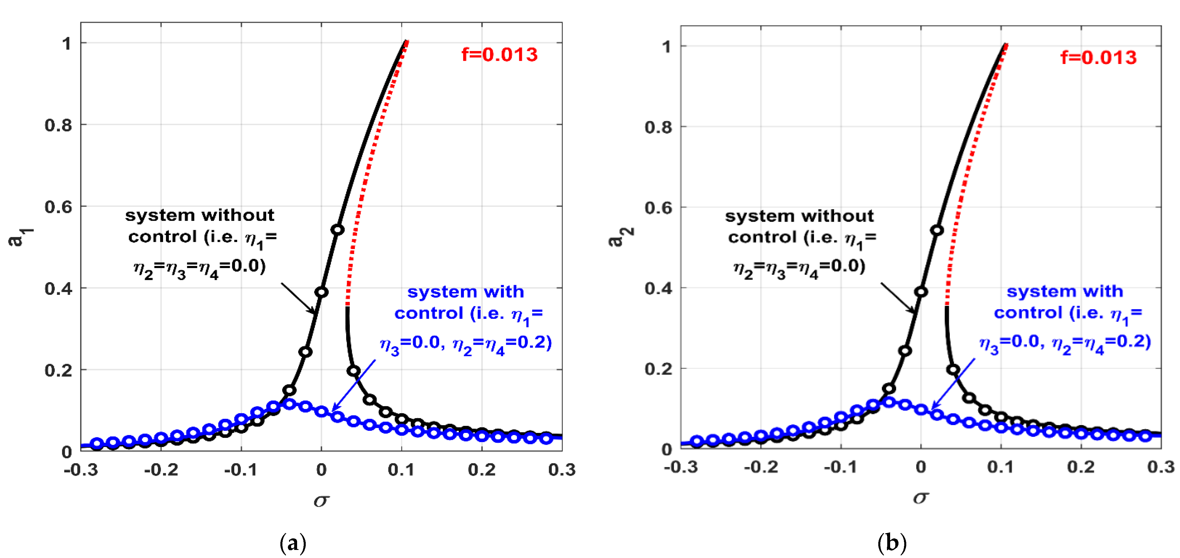
- When only the -control algorithm is activated, the twelve-poles rotor behaves like a hardening duffing oscillator, and the nonlinearities dominate its response when the rotor is exposed to a considerable excitation force amplitude (i.e., ) at the resonance condition. In addition, the electro-magnetic suspension system may suffer from rub and/or impact force between the rotor and the stator if in the case of -control algorithm.
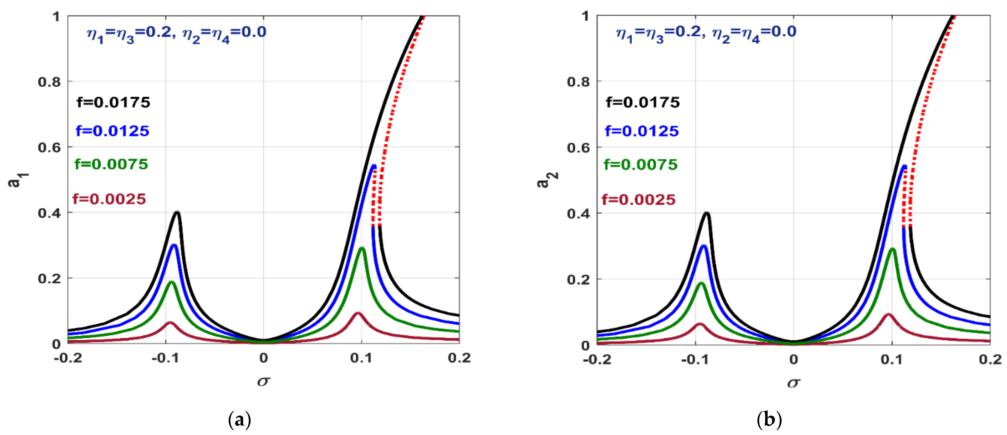
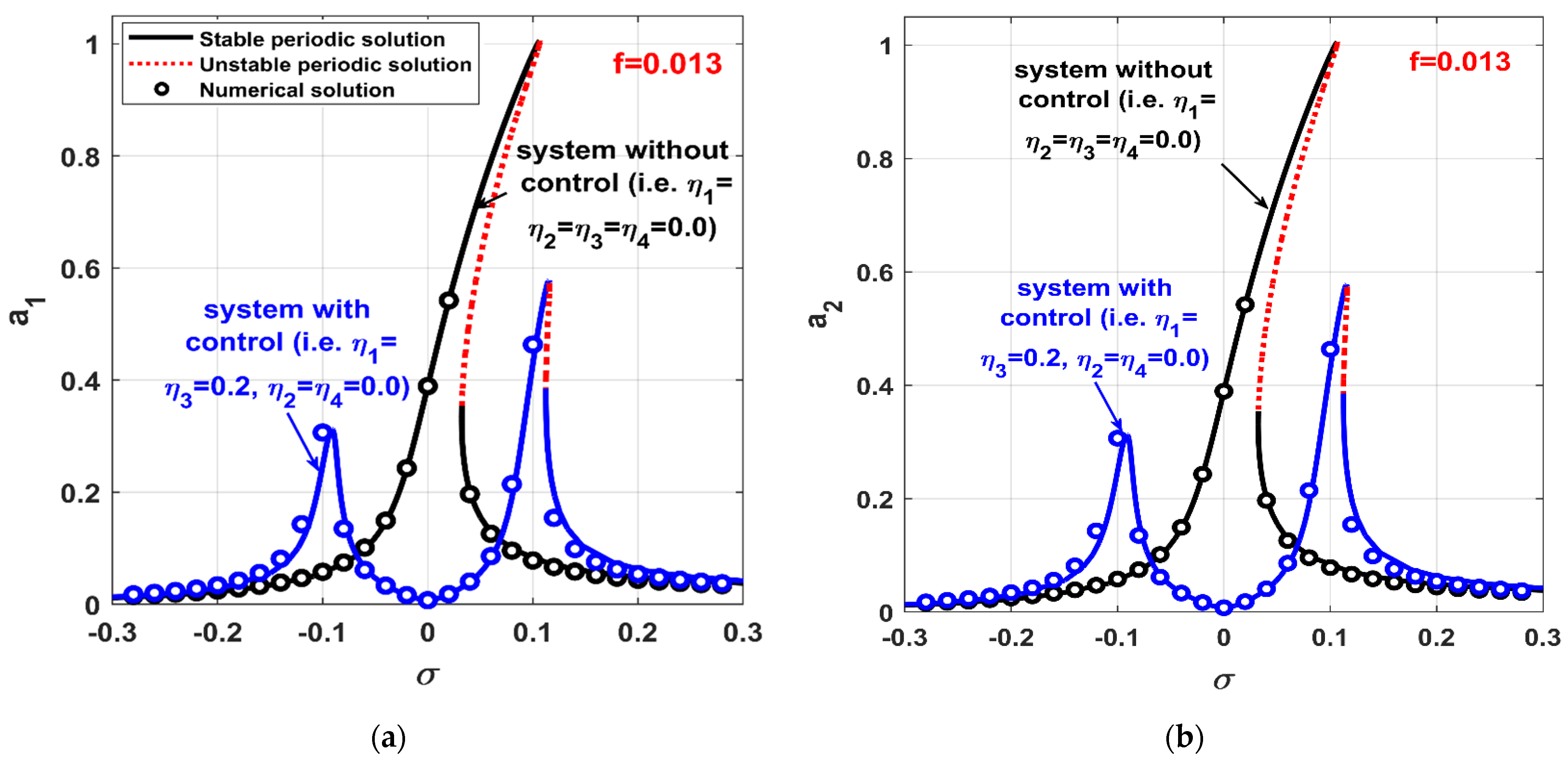
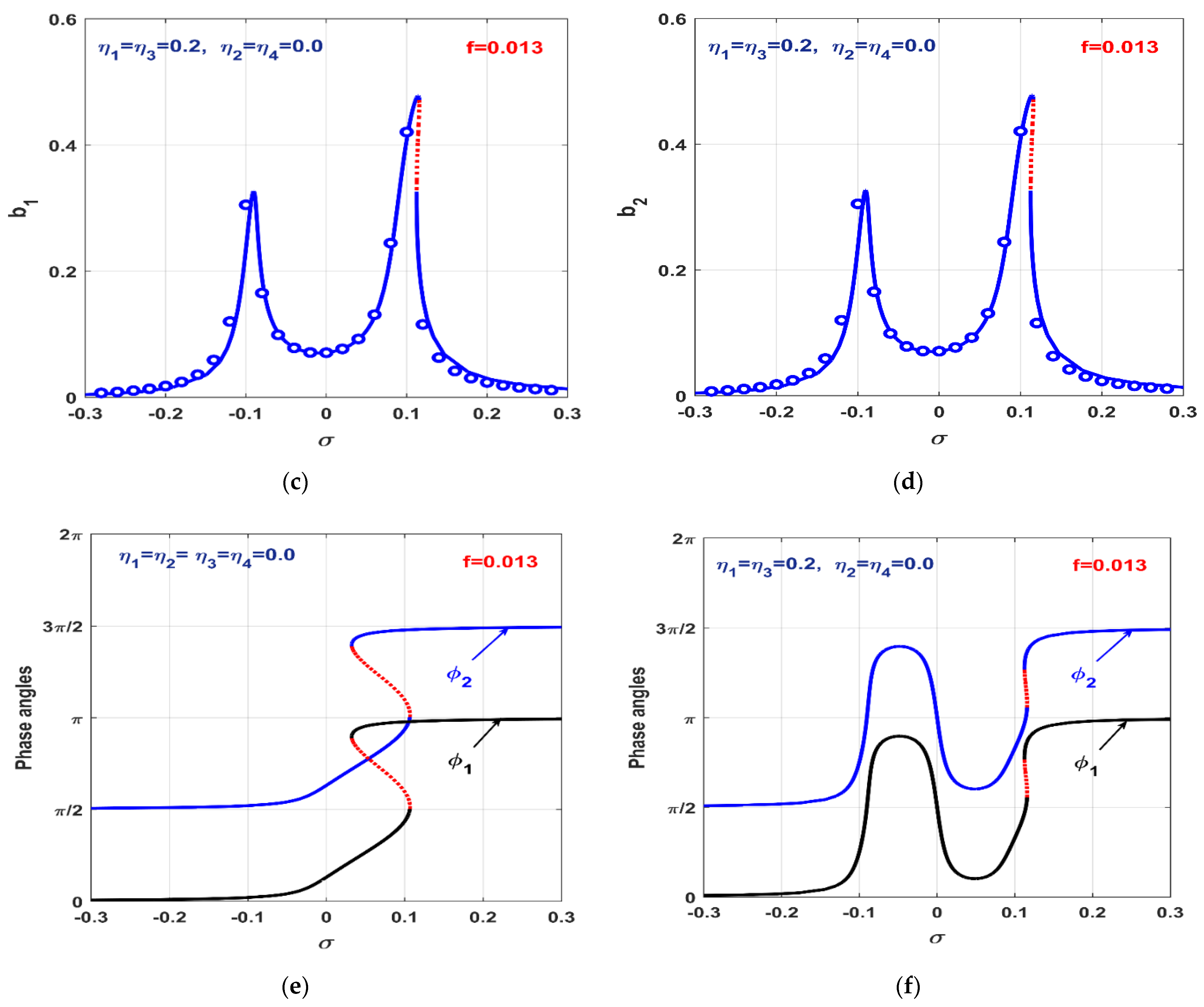
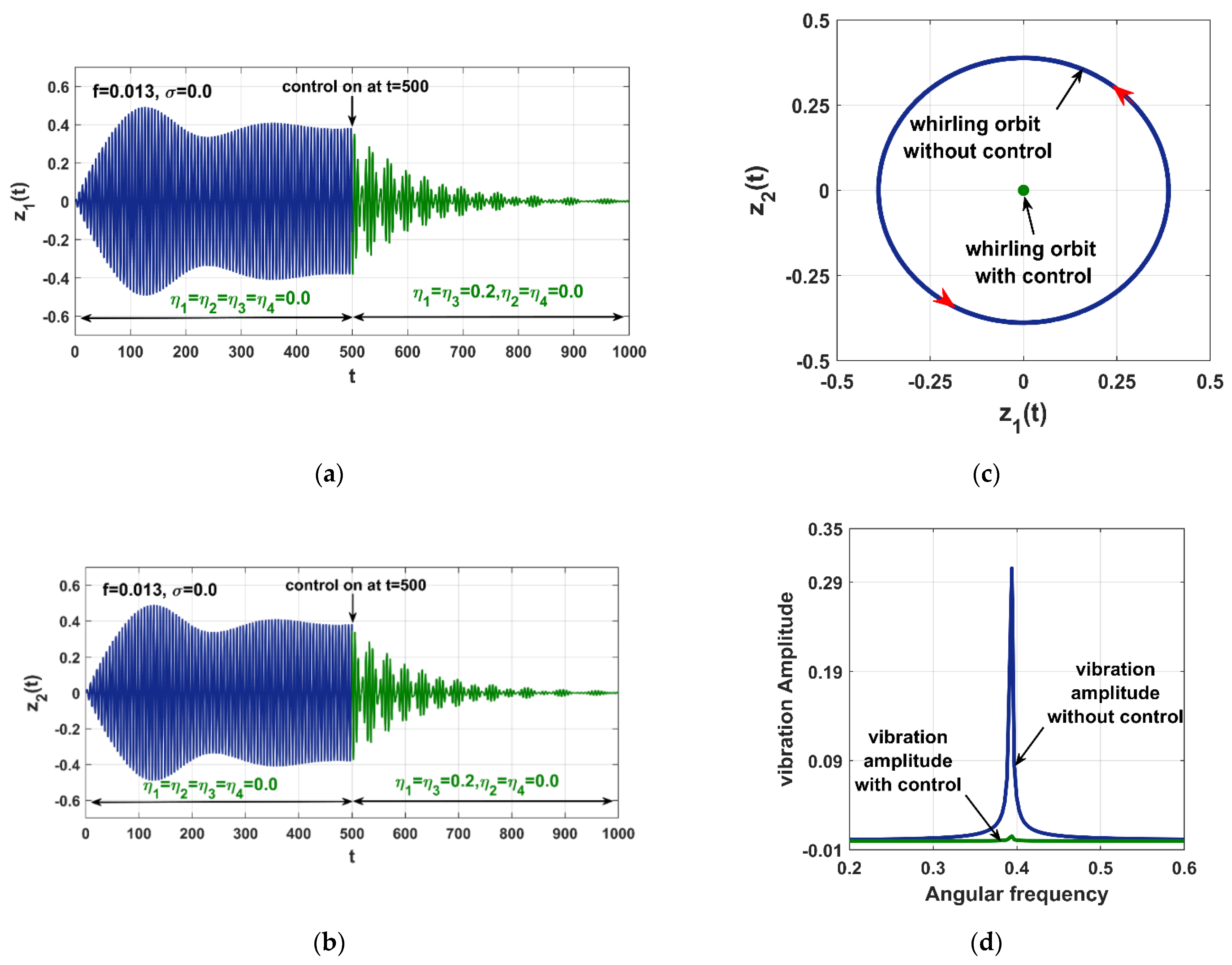
- Integrating the -control algorithm with -controller can eliminate the rotor’s undesired vibrations at the resonance condition (i.e., when ) to negligible oscillation amplitudes, regardless of the excitation force magnitude, but two undesired resonant peaks appear on both sides of that may result in high vibrations for the rotor system if the resonant condition is lost (i.e., if ).
- The -control algorithm can mitigate the undesired vibrations and eliminate the nonlinear bifurcation behaviors of the twelve-poles system. However, the main drawback of this controller is that the rotor may perform high oscillation amplitude at the perfect resonance (i.e., when ).
- Utilizing the three control algorithms (i.e., ) as one control strategy eliminated the high oscillation amplitudes of the rotor system close to zero at the perfect resonance conditions. In addition, the resonant peaks that appeared in the case of controller were also suppressed close to zero.
- The -control algorithm has all the advantages of the individual control algorithms, and , while avoiding their drawbacks.
- Although both the and -control algorithms can eliminate the nonlinear vibrations of the twelve-poles system at the perfect resonance condition, the has the advantage of having the short transient time in suppressing this undesired motion.
- Tuning the natural frequencies ( and ) of the -control algorithm to be close to or equal to the rotor angular speed () guarantees the elimination of the system’s lateral vibrations, regardless of the excitation force magnitude.
Author Contributions
Funding
Institutional Review Board Statement
Informed Consent Statement
Data Availability Statement
Acknowledgments
Conflicts of Interest
Abbreviations
| Normalized displacement, velocity, and acceleration of the twelve-poles system in the direction. | |
| Normalized displacement, velocity, and acceleration of the twelve-poles system in the direction. | |
| Normalized displacement, velocity, and acceleration of the -control algorithm that connected to the twelve-poles system in the direction. | |
| Normalized displacement, velocity, and acceleration of the -control algorithm that connected to the twelve-poles system in the direction. | |
| Normalized displacement, and velocity of the -control algorithm that connected to the twelve-poles system in the direction. | |
| Normalized displacement, and velocity of the -control algorithm that connected to the twelve-poles system in the direction. | |
| Normalized damping parameter of the twelve-poles rotor system. | |
| Normalized damping parameters of the -control algorithms. | |
| The normalized natural frequency of the twelve-poles rotor system. | |
| Normalized natural frequencies of the -control algorithms. | |
| Normalized Internal-loop feedback gains of the -control algorithms. | |
| The normalized angular speed of the twelve-poles rotor system. | |
| Normalized excitation force of the twelve-poles rotor system. | |
| Normalized proportional and derivative control gains of the -control algorithm, respectively. | |
| Normalized control gains of the -control algorithms. | |
| Normalized control gains of the -control algorithms. | |
| Normalized feedback gains of the -control algorithms. | |
| Normalized feedback gains of the -control algorithms. | |
| Normalized nonlinear coupling coefficients due to the -control algorithm. | |
| Normalized nonlinear coupling coefficients due to both the and control algorithms in the direction. | |
| Normalized nonlinear coupling coefficients due to both the and control algorithms in the direction. | |
| Normalized vibration amplitudes of the twelve-poles rotor system in the and directions, respectively. | |
| Phase angles of the twelve-poles rotor system in the and directions, respectively. | |
| Normalized vibration amplitudes of the -control algorithms in the and directions, respectively. | |
| Phase angles of the -control algorithms in the and directions, respectively. | |
| Difference between the angular speed () and the normalized natural frequency (: . |
Appendix A
Appendix B
Appendix C
References
- Ji, J.C.; Yu, L.; Leung, A.Y.T. Bifurcation behavior of a rotor supported by active magnetic bearings. J. Sound Vib. 2000, 235, 133–151. [Google Scholar] [CrossRef]
- Saeed, N.A.; Awwad, E.M.; El-Meligy, M.A.; Nasr, E.S.A. Radial Versus Cartesian Control Strategies to Stabilize the Non-linear Whirling Motion of the Six-Pole Rotor-AMBs. IEEE Access 2020, 8, 138859–138883. [Google Scholar] [CrossRef]
- Ji, J.C.; Hansen, C.H. Non-linear oscillations of a rotor in active magnetic bearings. J. Sound Vib. 2001, 240, 599–612. [Google Scholar] [CrossRef]
- Ji, J.C.; Leung, A.Y.T. Non-linear oscillations of a rotor-magnetic bearing system under superharmonic resonance conditions. Int. J. Non-Linear Mech. 2003, 38, 829–835. [Google Scholar] [CrossRef]
- El-Shourbagy, S.M.; Saeed, N.A.; Kamel, M.; Raslan, K.R.; Abouel Nasr, E.; Awrejcewicz, J. On the Performance of a Non-linear Position-Velocity Controller to Stabilize Rotor-Active Magnetic-Bearings System. Symmetry 2021, 13, 2069. [Google Scholar] [CrossRef]
- Saeed, N.A.; Mahrous, E.; Abouel Nasr, E.; Awrejcewicz, J. Non-linear dynamics and motion bifurcations of the rotor active magnetic bearings system with a new control scheme and rub-impact force. Symmetry 2021, 13, 1502. [Google Scholar] [CrossRef]
- Zhang, W.; Zhan, X.P. Periodic and chaotic motions of a rotor-active magnetic bearing with quadratic and cubic terms and time-varying stiffness. Nonlinear Dyn. 2005, 41, 331–359. [Google Scholar] [CrossRef]
- Zhang, W.; Yao, M.H.; Zhan, X.P. Multi-pulse chaotic motions of a rotor-active magnetic bearing system with time-varying stiffness. Chaos Solitons Fractals 2006, 27, 175–186. [Google Scholar] [CrossRef]
- Zhang, W.; Zu, J.W.; Wang, F.X. Global bifurcations and chaos for a rotor-active magnetic bearing system with time-varying stiffness. Chaos Solitons Fractals 2008, 35, 586–608. [Google Scholar] [CrossRef]
- Zhang, W.; Zu, J.W. Transient and steady non-linear responses for a rotor-active magnetic bearings system with time-varying stiffness. Chaos Solitons Fractals 2008, 38, 1152–1167. [Google Scholar] [CrossRef]
- Li, J.; Tian, Y.; Zhang, W.; Miao, S.F. Bifurcation of multiple limit cycles for a rotor-active magnetic bearings system with time-varying stiffness. Int. J. Bifurc. Chaos 2008, 18, 755–778. [Google Scholar] [CrossRef]
- Li, J.; Tian, Y.; Zhang, W. Investigation of relation between singular points and number of limit cycles for a rotor–AMBs system. Chaos Solitons Fractals 2009, 39, 1627–1640. [Google Scholar] [CrossRef]
- El-Shourbagy, S.M.; Saeed, N.A.; Kamel, M.; Raslan, K.R.; Aboudaif, M.K.; Awrejcewicz, J. Control Performance, Stability Conditions, and Bifurcation Analysis of the Twelve-pole Active Magnetic Bearings System. Appl. Sci. 2021, 11, 10839. [Google Scholar] [CrossRef]
- Saeed, N.A.; Kandil, A. Two different control strategies for 16-pole rotor active magnetic bearings system with constant stiffness coefficients. Appl. Math. Model. 2021, 92, 1–22. [Google Scholar] [CrossRef]
- Wu, R.; Zhang, W.; Yao, M.H. Analysis of non-linear dynamics of a rotor-active magnetic bearing system with 16-pole legs. In Proceedings of the International Design Engineering Technical Conferences and Computers and Information in Engineering Conference, Cleveland, OH, USA, 6–9 August 2017. [Google Scholar] [CrossRef]
- Wu, R.Q.; Zhang, W.; Yao, M.H. Non-linear dynamics near resonances of a rotor-active magnetic bearings system with 16-pole legs and time varying stiffness. Mech. Syst. Signal Process. 2018, 100, 113–134. [Google Scholar] [CrossRef]
- Zhang, W.; Wu, R.Q.; Siriguleng, B. Non-linear Vibrations of a Rotor-Active Magnetic Bearing System with 16-Pole Legs and Two Degrees of Freedom. Shock. Vib. 2020, 2020, 5282904. [Google Scholar]
- Ma, W.S.; Zhang, W.; Zhang, Y.F. Stability and multi-pulse jumping chaotic vibrations of a rotor-active magnetic bearing system with 16-pole legs under mechanical-electric-electro-magnetic excitations. Eur. J. Mech. A/Solids 2021, 85, 104120. [Google Scholar] [CrossRef]
- Ishida, Y.; Inoue, T. Vibration suppression of non-linear rotor systems using a dynamic damper. J. Vib. Control. 2007, 13, 1127–1143. [Google Scholar] [CrossRef]
- Saeed, N.A.; Awwad, E.M.; El-Meligy, M.A.; Nasr, E.S.A. Sensitivity analysis and vibration control of asymmetric non-linear rotating shaft system utilizing 4-pole AMBs as an actuator. Eur. J. Mech. A/Solids 2021, 86, 104145. [Google Scholar] [CrossRef]
- Saeed, N.A.; Eissa, M. Bifurcation analysis of a transversely cracked non-linear Jeffcott rotor system at different resonance cases. Int. J. Acoust. Vib. 2019, 24, 284–302. [Google Scholar] [CrossRef]
- Saeed, N.A.; Awwad, E.M.; El-Meligy, M.A.; Nasr, E.S.A. Analysis of the rub-impact forces between a controlled non-linear rotating shaft system and the electromagnet pole legs. Appl. Math. Model. 2021, 93, 792–810. [Google Scholar] [CrossRef]
- Srinivas, R.S.; Tiwari, R.; Kannababu, C. Application of active magnetic bearings in flexible rotordynamic systems—A state-of-the-art review. Mech. Syst. Signal Processing 2018, 106, 537–572. [Google Scholar] [CrossRef]
- Shan, J.; Liu, H.; Sun, D. Slewing and vibration control of a single-link flexible manipulator by positive position feedback (PPF). Mechatronics 2005, 15, 487–503. [Google Scholar] [CrossRef]
- Ahmed, B.; Pota, H.R. Dynamic compensation for control of a rotary wing UAV using positive position feedback. J. Intell. Robot. Syst. 2011, 61, 43–56. [Google Scholar] [CrossRef]
- Warminski, J.; Bochenski, M.; Jarzyna, W.; Filipek, P.; Augustyinak, M. Active suppression of non-linear composite beam vibrations by selected control algorithms. Commun. Nonlinear Sci. Numer. Simul. 2011, 16, 2237–2248. [Google Scholar] [CrossRef]
- Omidi, E.; Mahmoodi, S.N. Non-linear vibration suppression of flexible structures using non-linear modified positive position feedback approach. Nonlinear Dyn. 2015, 79, 835–849. [Google Scholar] [CrossRef]
- Saeed, N.A.; Kandil, A. Lateral vibration control and stabilization of the quasiperiodic oscillations for rotor-active magnetic bearings system. Nonlinear Dyn. 2019, 98, 1191–1218. [Google Scholar] [CrossRef]
- Diaz, I.M.; Pereira, E.; Reynolds, P. Integral resonant control scheme for cancelling human-induced vibrations in light-weight pedestrian structures. Struct. Control Health Monit 2012, 19, 55–69. [Google Scholar] [CrossRef]
- Al-Mamun, A.; Keikha, E.; Bhatia, C.S.; Lee, T.H. Integral resonant control for suppression of resonance in piezoelectric micro-actuator used in precision servomechanism. Mechatronics 2013, 23, 1–9. [Google Scholar] [CrossRef]
- Omidi, E.; Mahmoodi, S.N. Non-linear integral resonant controller for vibration reduction in non-linear systems. Acta Mech. Sin 2016, 32, 925–934. [Google Scholar] [CrossRef]
- MacLean, J.D.J.; Sumeet, S.A. A modified linear integral resonant controller for suppressing jump phenomenon and hysteresis in micro-cantilever beam structures. J. Sound Vib. 2020, 480, 115365. [Google Scholar] [CrossRef]
- Omidi, E.; Mahmoodi, S.N. Sensitivity analysis of the Non-linear Integral Positive Position Feedback and Integral Resonant controllers on vibration suppression of non-linear oscillatory systems. Commun. Nonlinear Sci. Numer. Simul. 2015, 22, 149–166. [Google Scholar] [CrossRef]
- Saeed, N.A.; El-Shourbagy, S.M.; Kamel, M.; Raslan, K.R.; Aboudaif, M.K. Nonlinear Dynamics and Static Bifurcations Control of the 12-Pole Magnetic Bearings System Utilizing the Integral Resonant Control strategy. J. Low Freq. Noise Vib. Act. Control 2022. [Google Scholar] [CrossRef]
- Saeed, N.A.; Moatimid, G.M.; Elsabaa, F.M.; Ellabban, Y.Y.; Elagan, S.K.; Mohamed, M.S. Time-Delayed Non-linear Integral Resonant Controller to Eliminate the Non-linear Oscillations of a Parametrically Excited System. IEEE Access 2021, 9, 74836–74854. [Google Scholar] [CrossRef]
- Saeed, N.A.; Mohamed, M.S.; Elagan, S.K.; Awrejcewicz, J. Integral Resonant Controller to Suppress the Non-linear Oscillations of a Two-Degree-of-Freedom Rotor Active Magnetic Bearing System. Processes 2022, 10, 271. [Google Scholar] [CrossRef]
- Ishida, Y.; Yamamoto, T. Linear and Non-Linear Rotordynamics: A Modern Treatment with Applications, 2nd ed.; Wiley-VCH Verlag GmbH & Co. KGaA: New York, NY, USA, 2012. [Google Scholar]
- Schweitzer, G.; Maslen, E.H. Magnetic Bearings: Theory, Design, and Application to Rotating Machinery; Springer: Berlin/Heidelberg, Germany, 2009. [Google Scholar]
- Nayfeh, A.H.; Mook, D.T. Non-Linear Oscillations; Wiley: New York, NY, USA, 1995. [Google Scholar]
- Nayfeh, A.H. Resolving Controversies in the Application of the Method of Multiple Scales and the Generalized Method of Averaging. Nonlinear Dyn. 2005, 40, 61–102. [Google Scholar] [CrossRef]
- Vlase, S.; Năstac, C.; Marin, M.; Mihălcică, M. A method for the study of the vibration of mechanical bars systems with symmetries. Acta Tech. Napoc. 2017, 60, 539–544. [Google Scholar]
- Slotine, J.-J.E.; Li, W. Applied Non-Linear Control; Prentice Hall: Englewood Cliffs, NJ, USA, 1991. [Google Scholar]
- Yang, W.Y.; Cao, W.; Chung, T.; Morris, J. Applied Numerical Methods Using Matlab; John Wiley & Sons, Inc.: Hoboken, NJ, USA, 2005. [Google Scholar]


Publisher’s Note: MDPI stays neutral with regard to jurisdictional claims in published maps and institutional affiliations. |
© 2022 by the authors. Licensee MDPI, Basel, Switzerland. This article is an open access article distributed under the terms and conditions of the Creative Commons Attribution (CC BY) license (https://creativecommons.org/licenses/by/4.0/).
Share and Cite
Saeed, N.A.; El-Shourbagy, S.M.; Kamel, M.; Raslan, K.R.; Awrejcewicz, J.; Gepreel, K.A. On the Resonant Vibrations Control of the Nonlinear Rotor Active Magnetic Bearing Systems. Appl. Sci. 2022, 12, 8300. https://0-doi-org.brum.beds.ac.uk/10.3390/app12168300
Saeed NA, El-Shourbagy SM, Kamel M, Raslan KR, Awrejcewicz J, Gepreel KA. On the Resonant Vibrations Control of the Nonlinear Rotor Active Magnetic Bearing Systems. Applied Sciences. 2022; 12(16):8300. https://0-doi-org.brum.beds.ac.uk/10.3390/app12168300
Chicago/Turabian StyleSaeed, Nasser A., Sabry M. El-Shourbagy, Magdi Kamel, Kamal R. Raslan, Jan Awrejcewicz, and Khaled A. Gepreel. 2022. "On the Resonant Vibrations Control of the Nonlinear Rotor Active Magnetic Bearing Systems" Applied Sciences 12, no. 16: 8300. https://0-doi-org.brum.beds.ac.uk/10.3390/app12168300