
Assessing the Seismic Demands on Non-Structural Components Attached to Reinforced Concrete Frames

 , , , and
Abstract
:1. Introduction
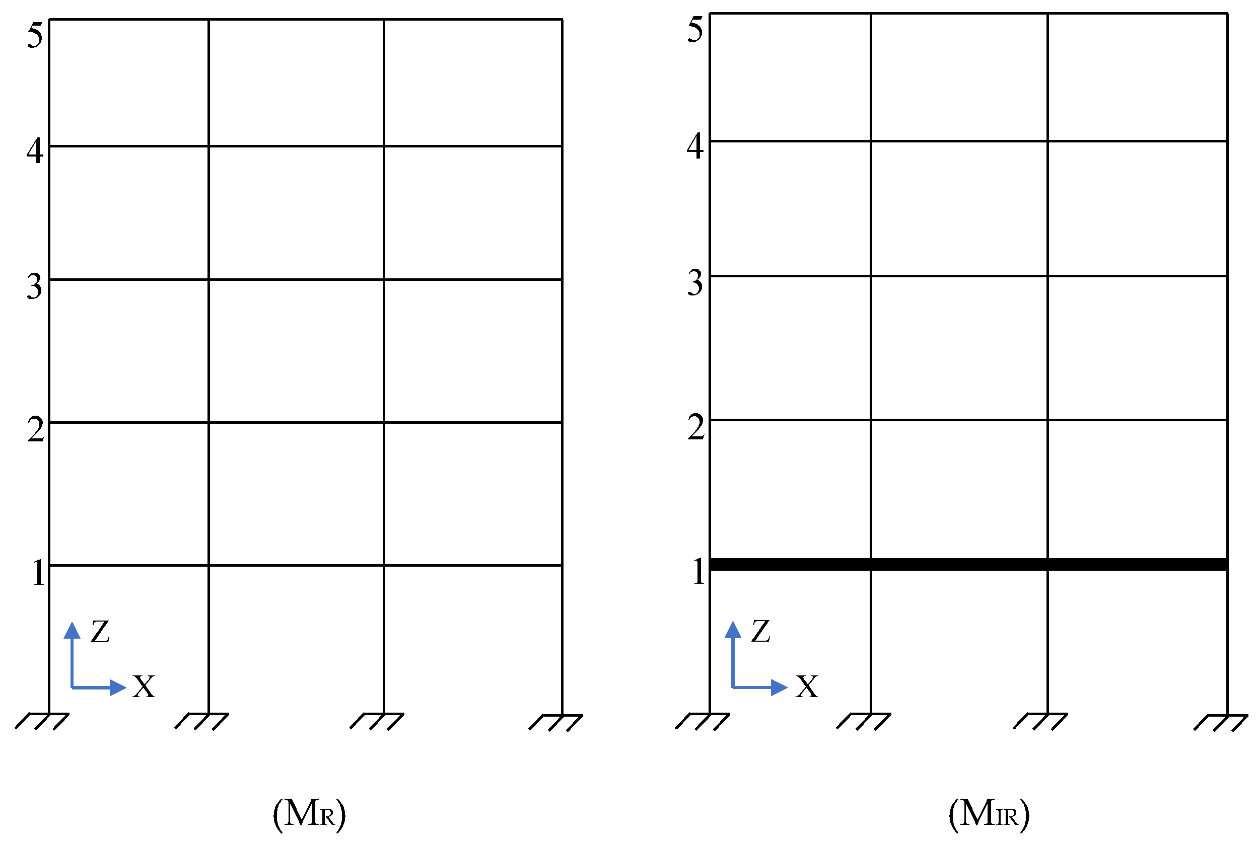
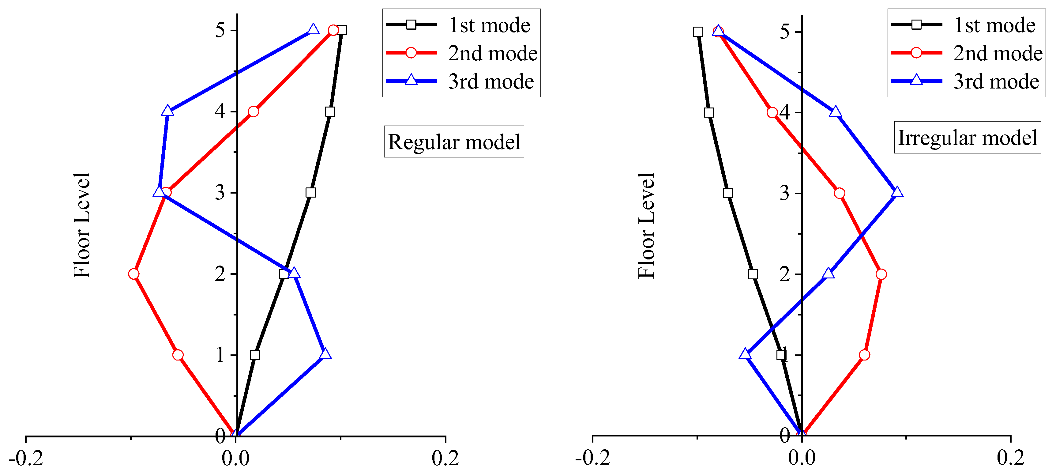
2. Modeling and Analysis of Buildings
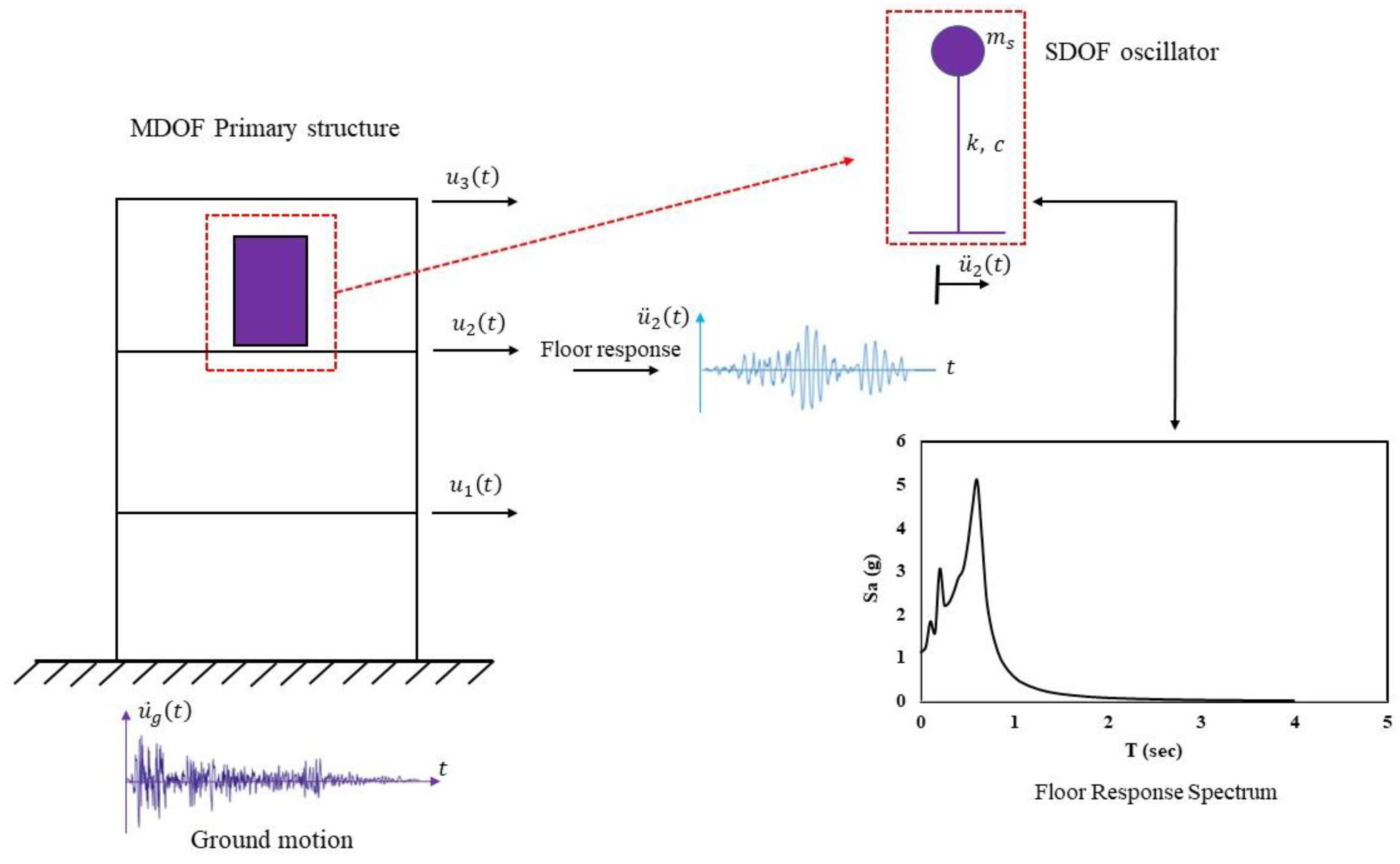
3. Generation of FRS
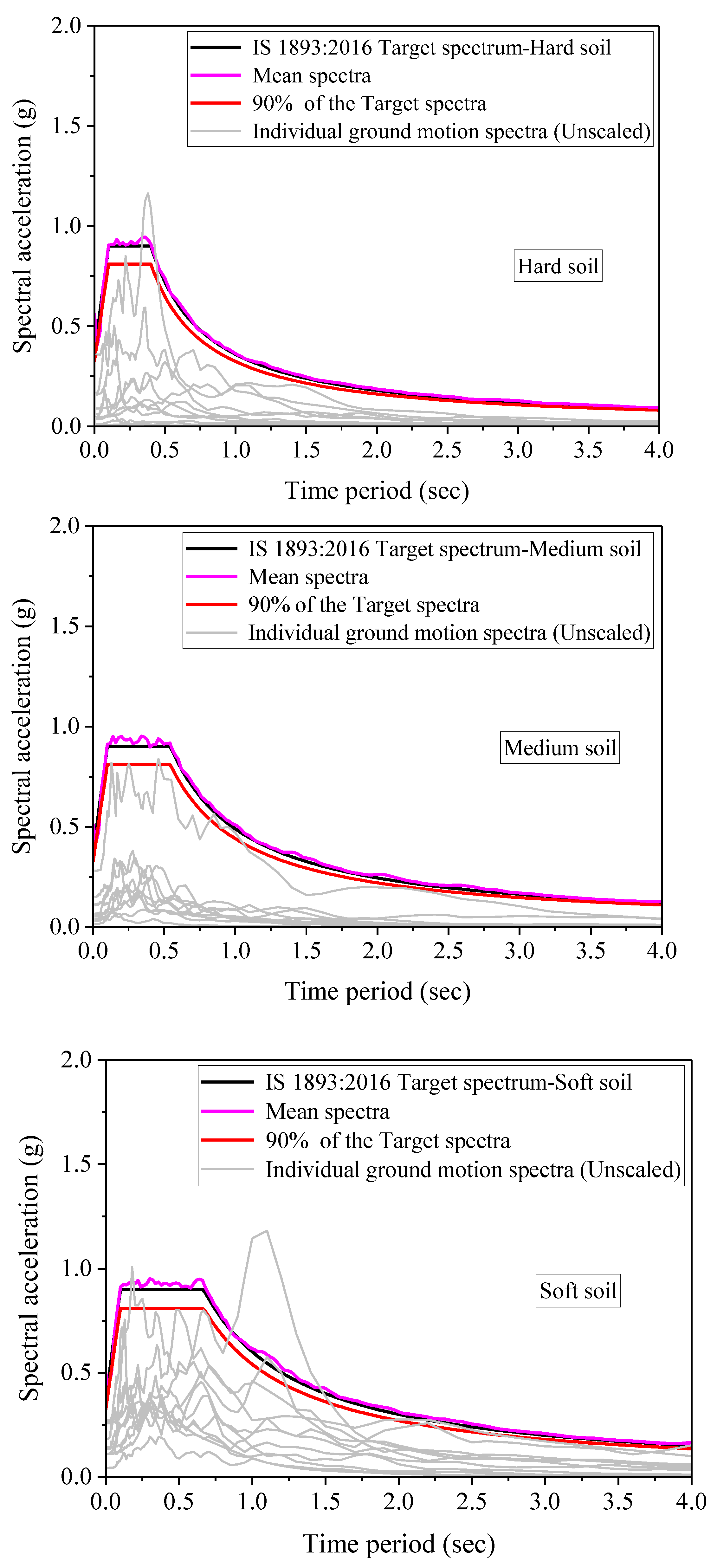
4. Selection and Scaling of Ground Motions
5. Results and Discussion
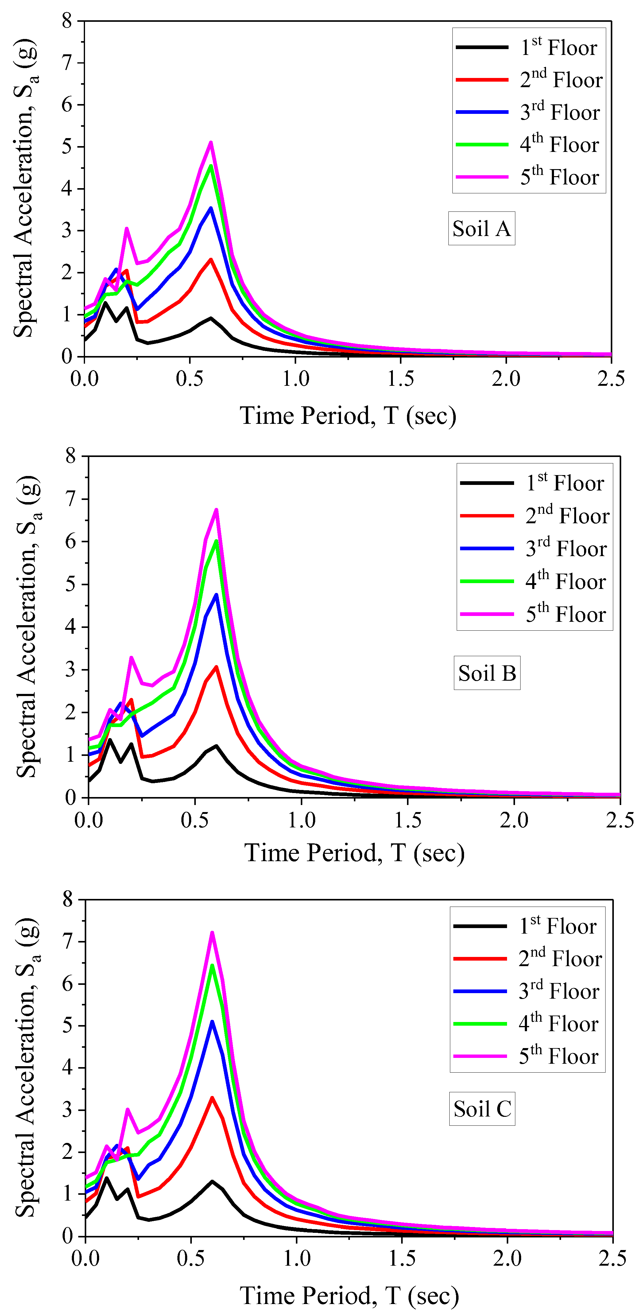
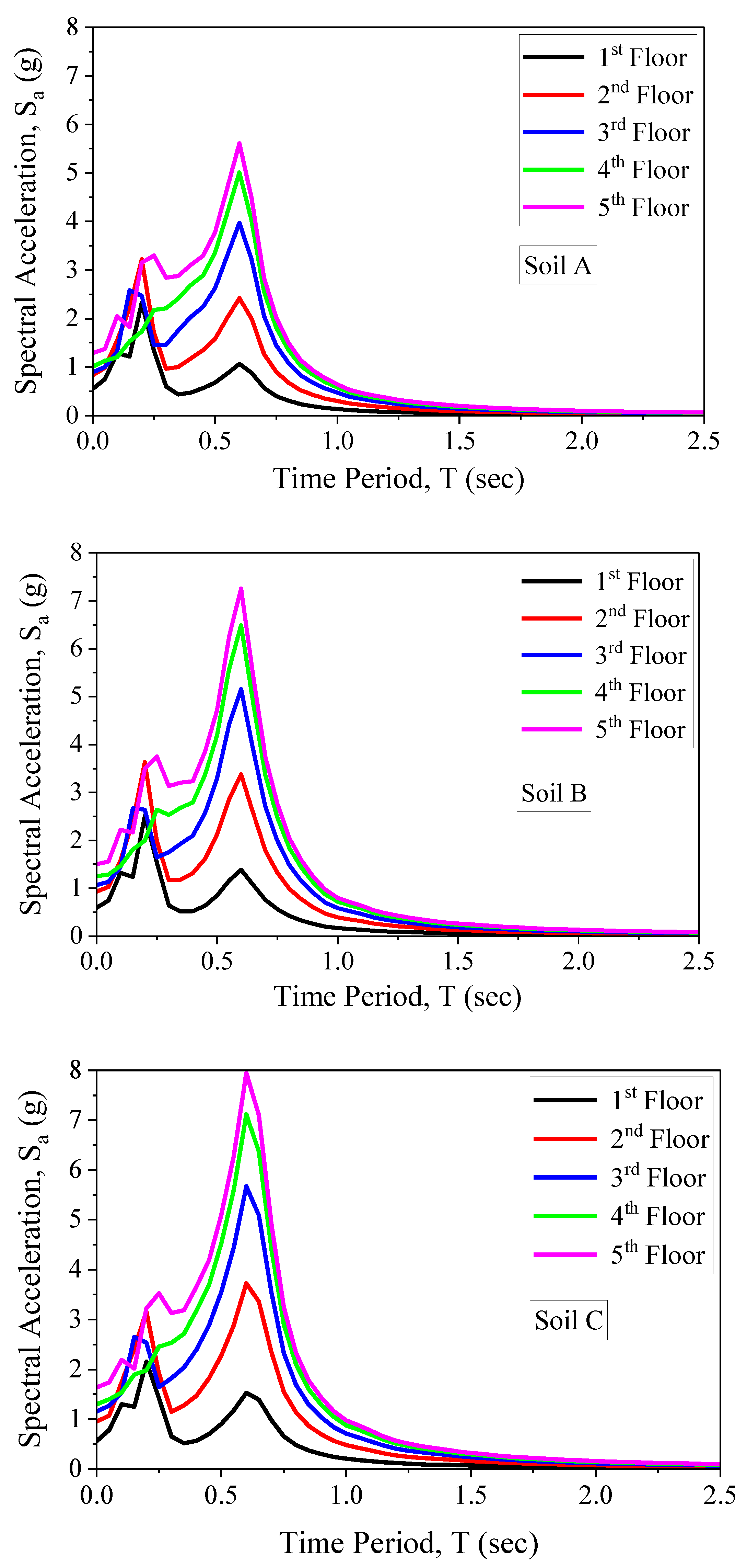
5.1. Elastic FRS for Regular and Irregular Buildings
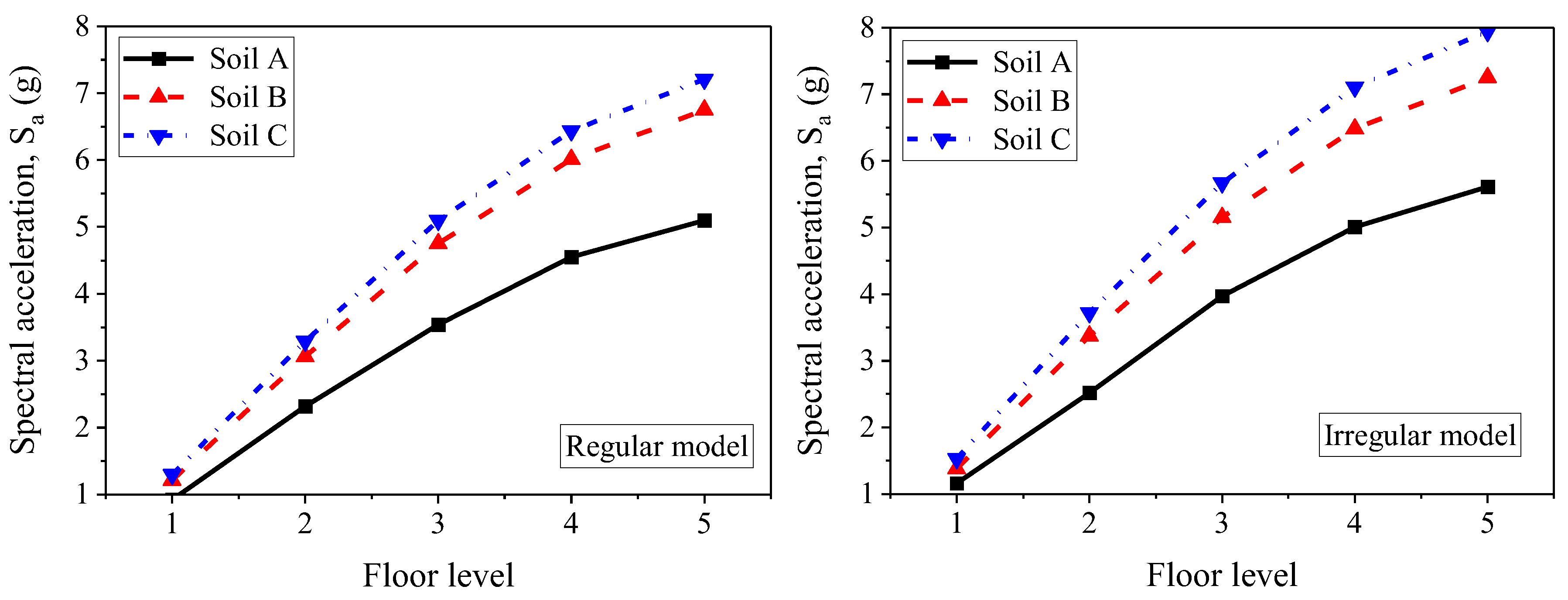
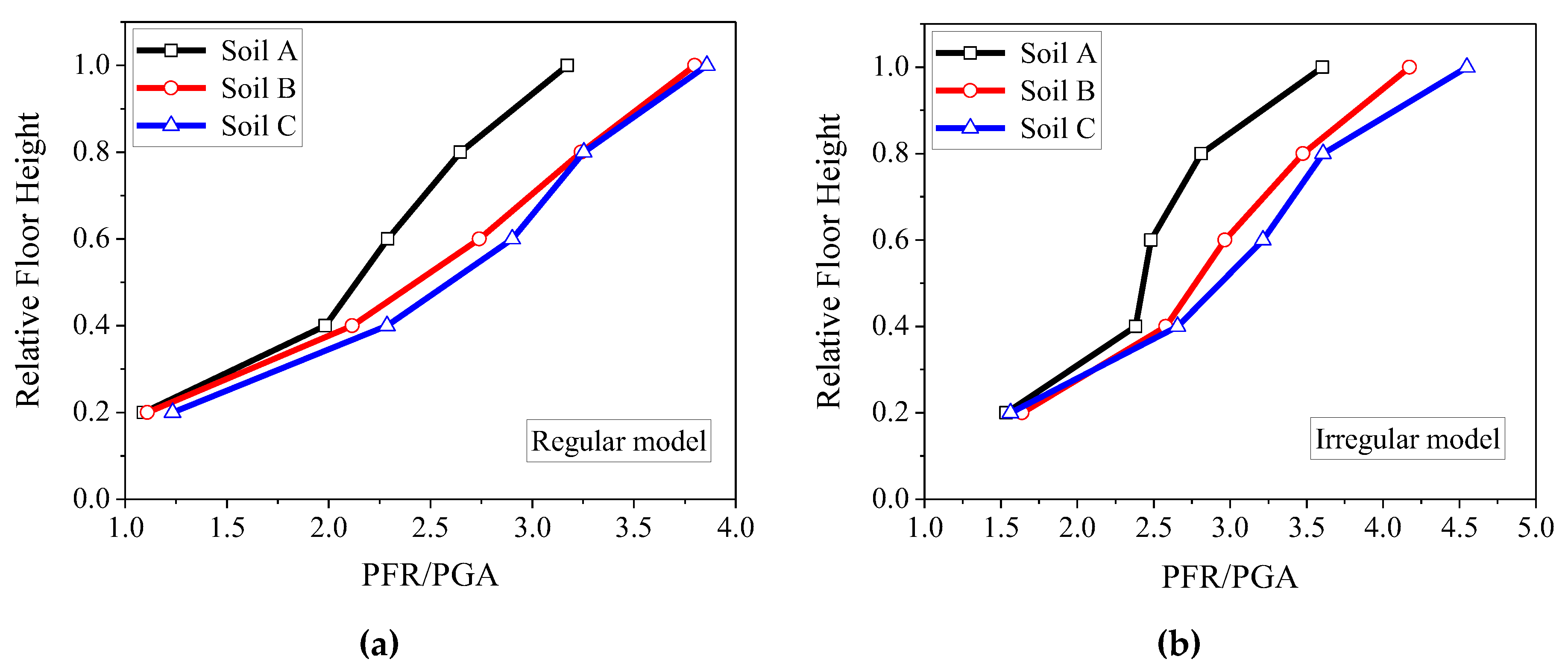
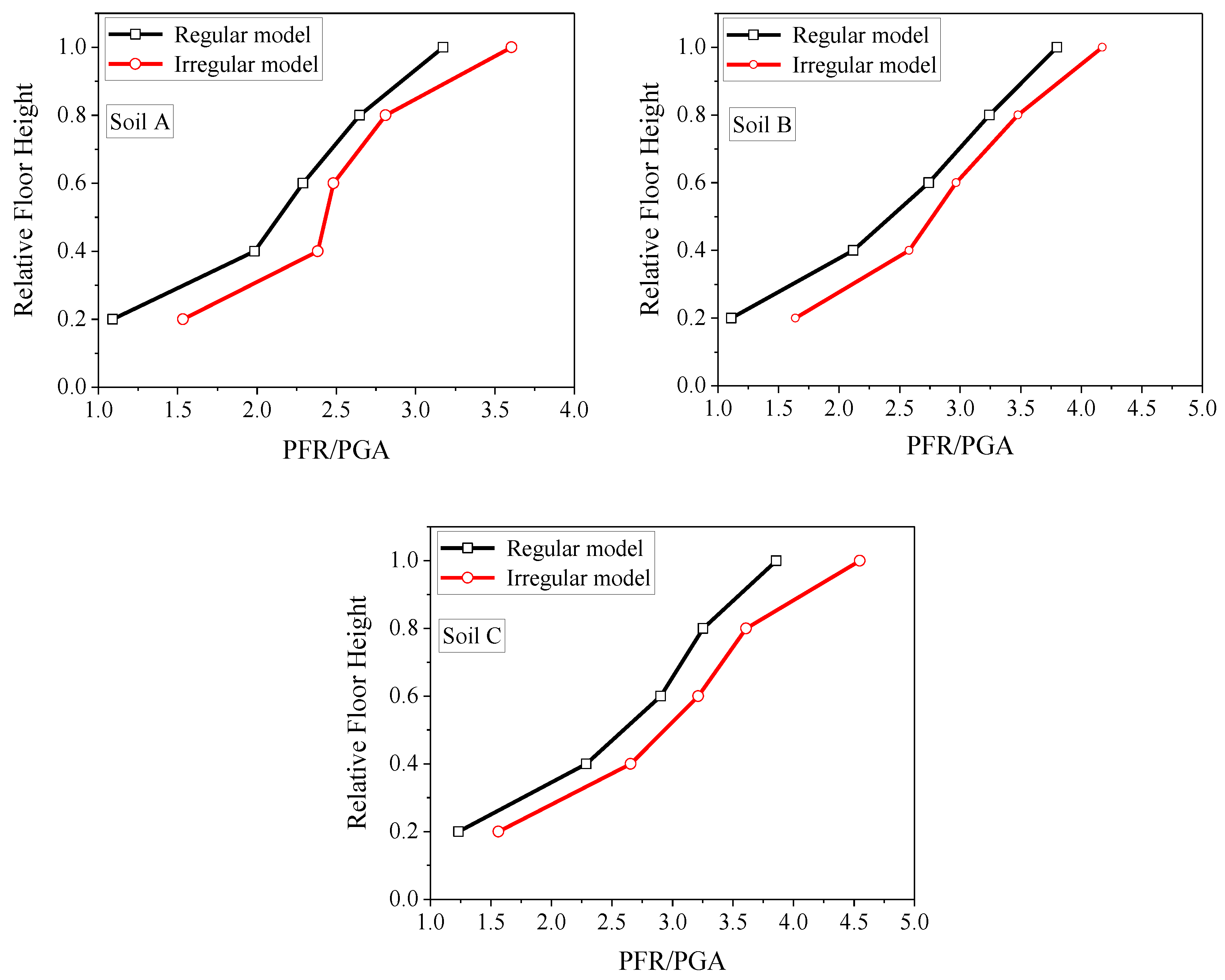
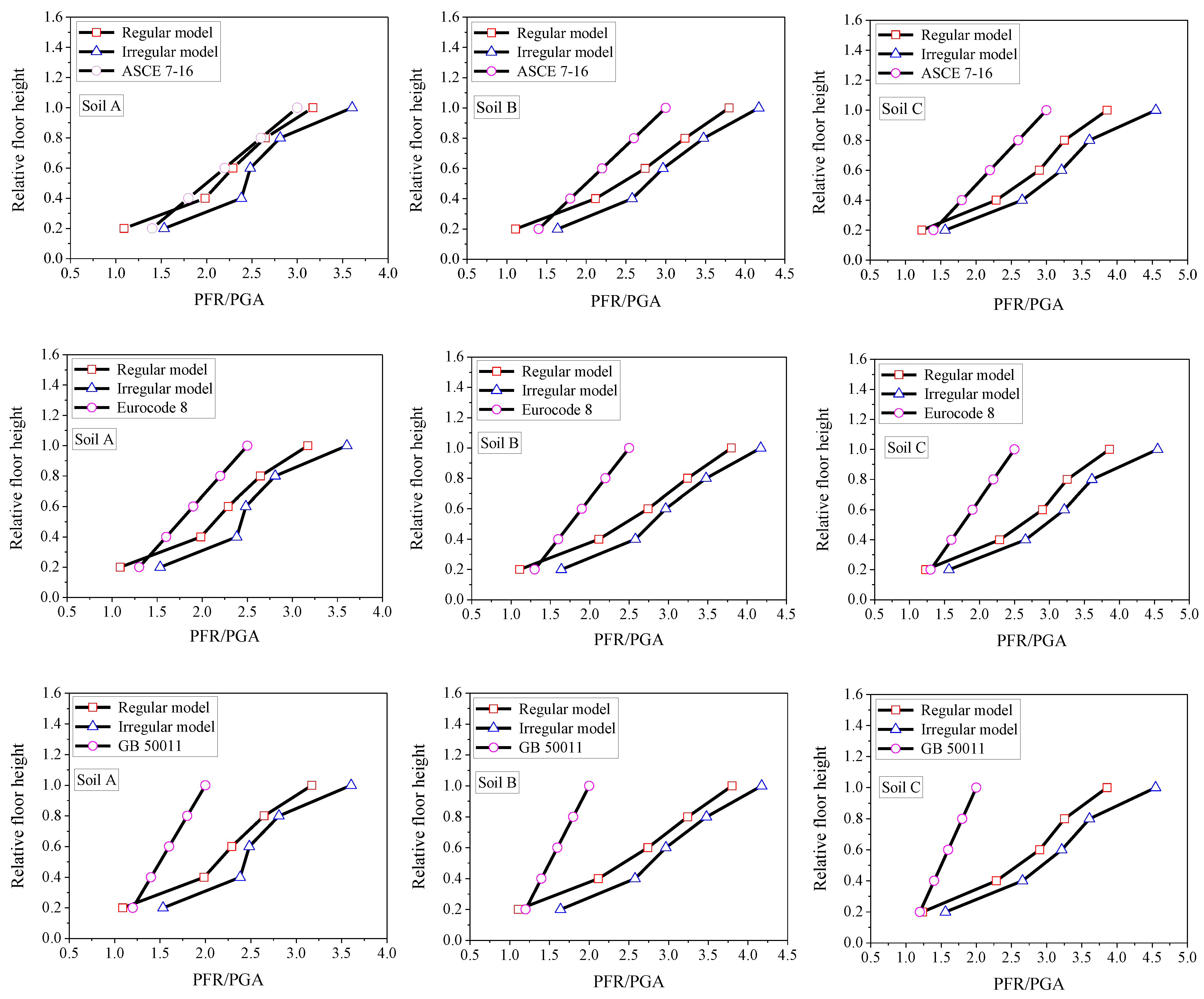
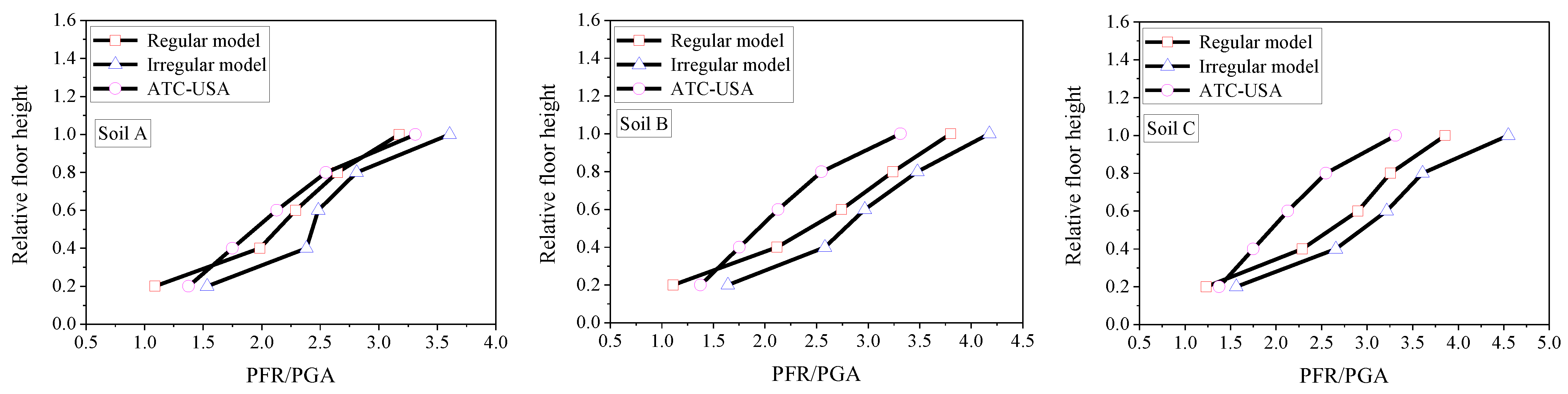
5.2. Normalized Floor Amplification
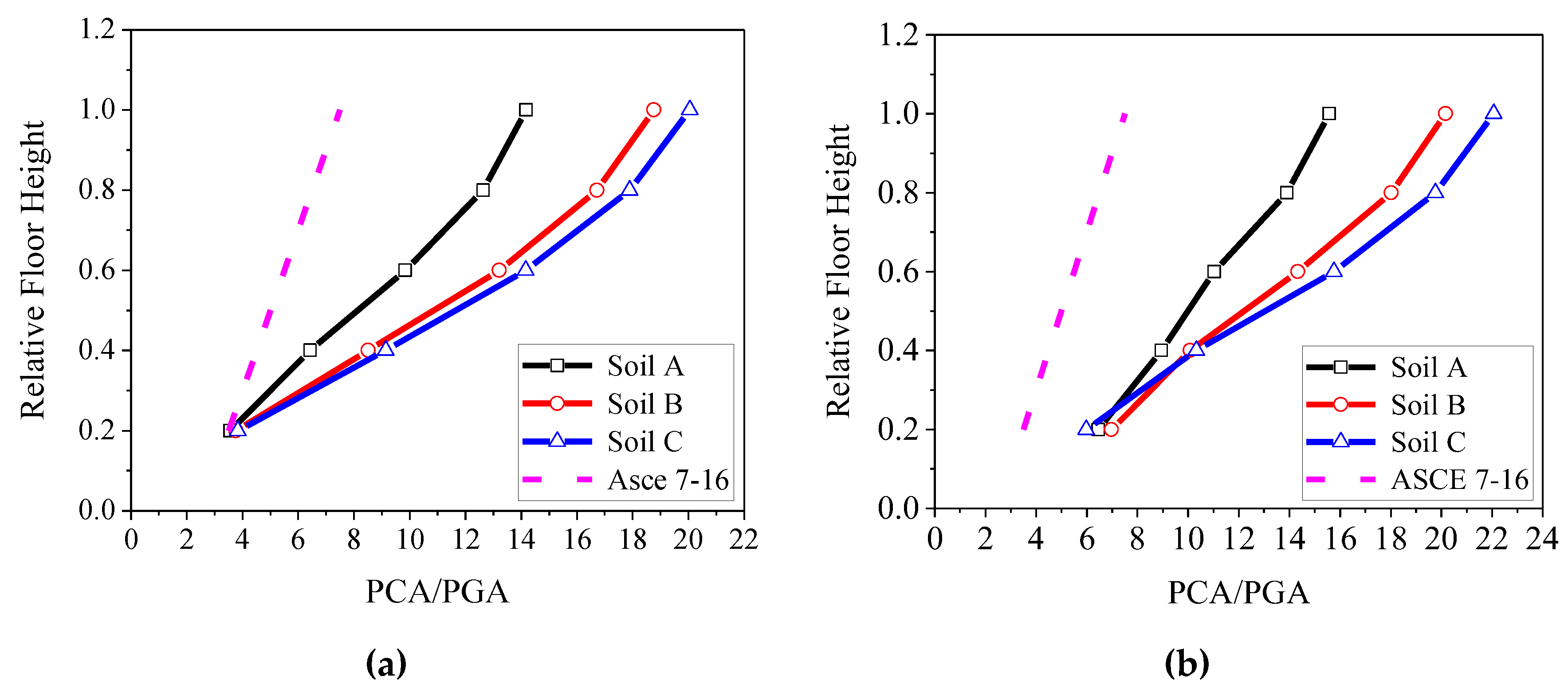
5.3. Peak Component Acceleration
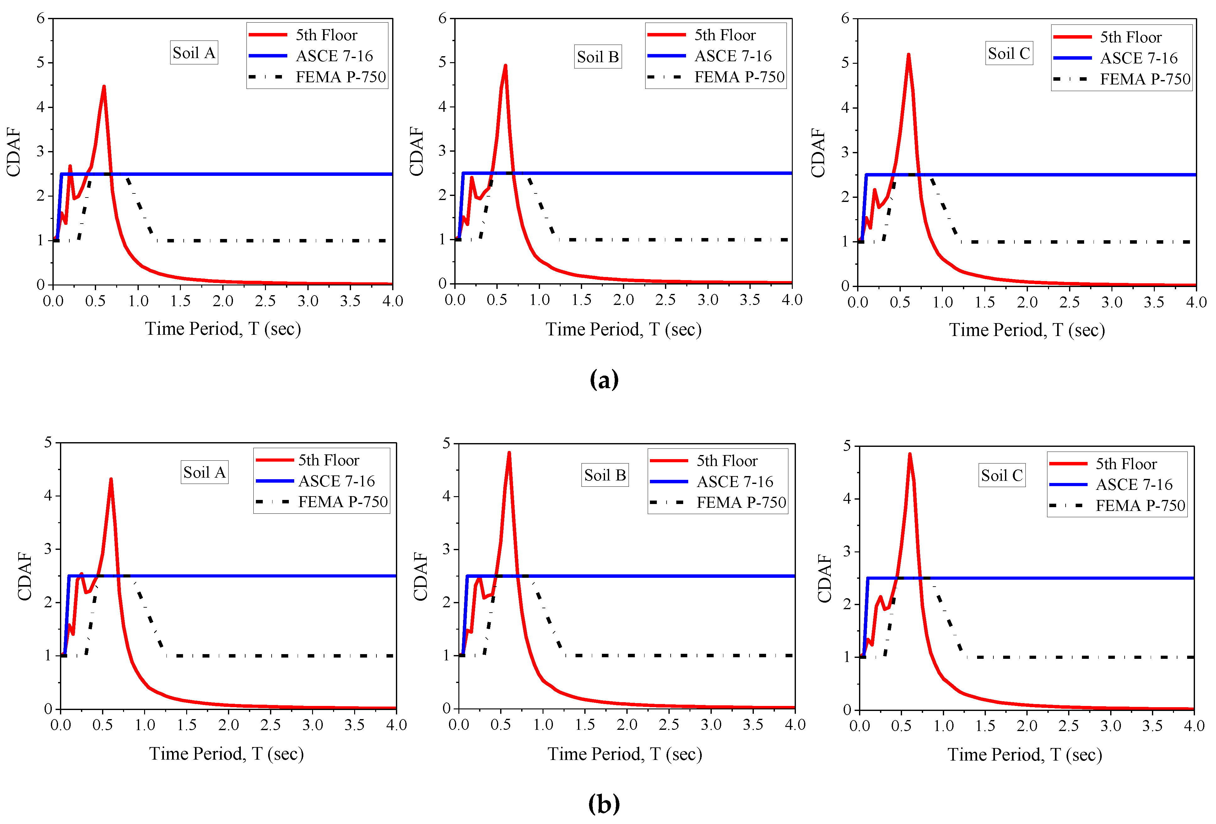
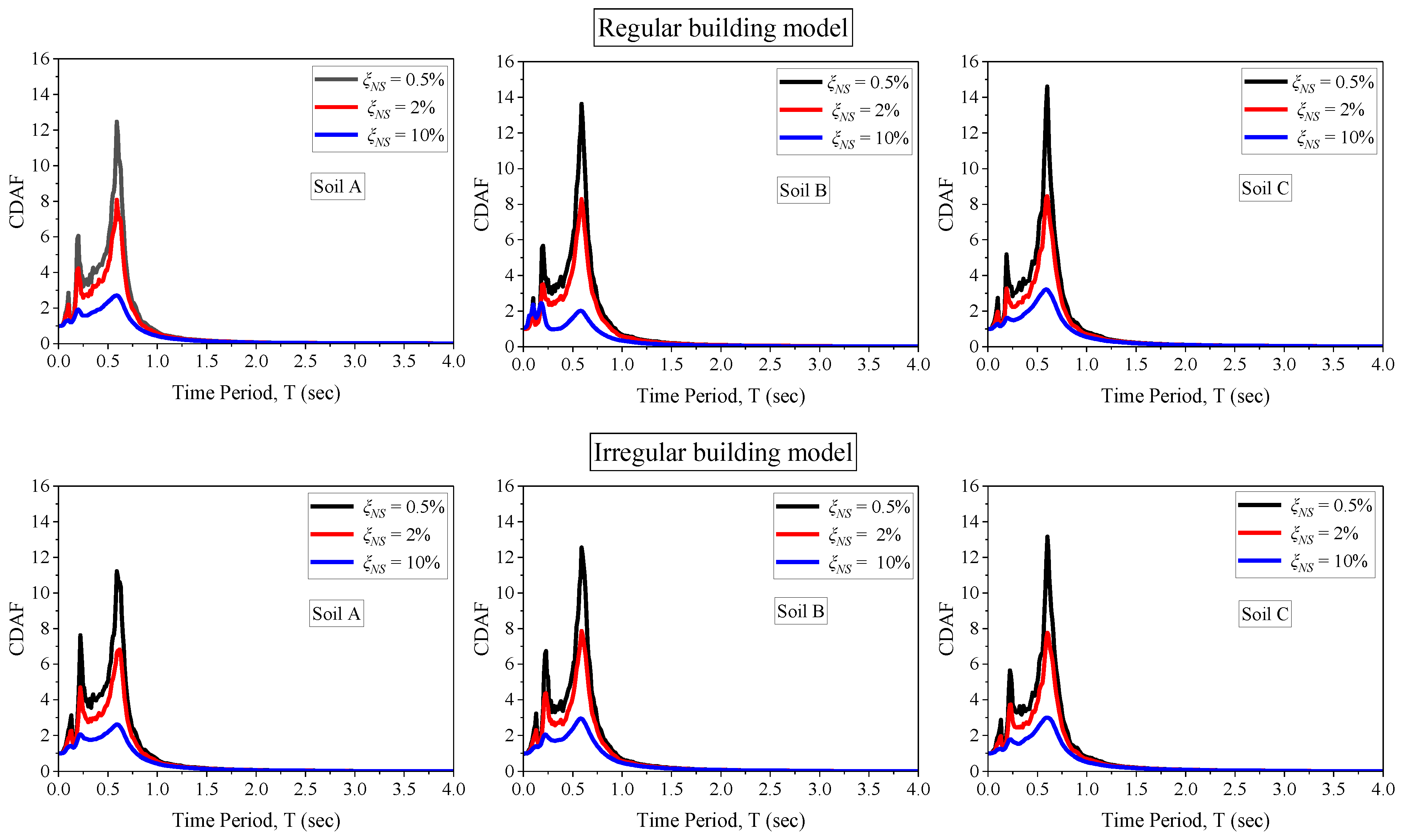
5.4. Component Dynamic Amplification Factor
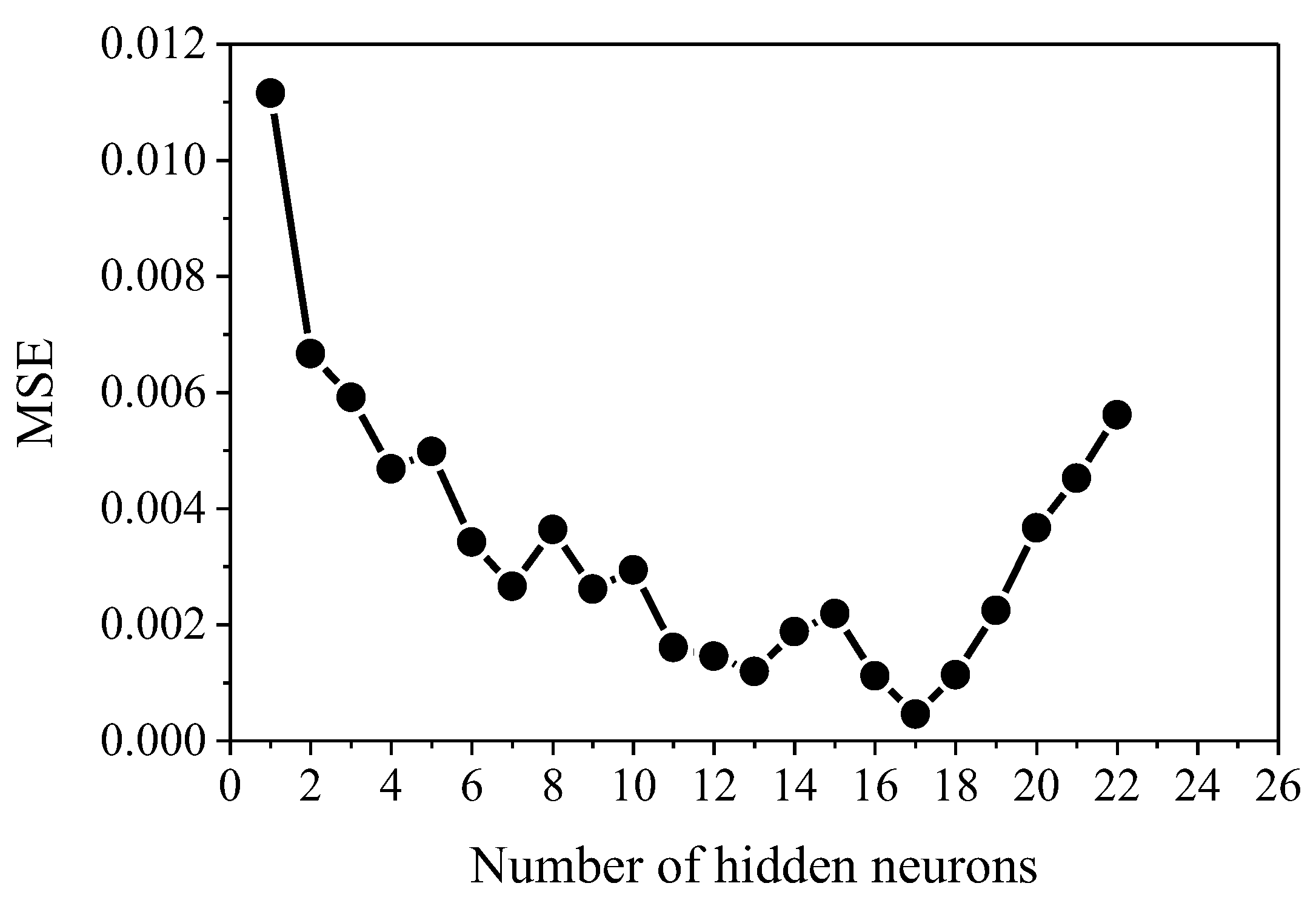
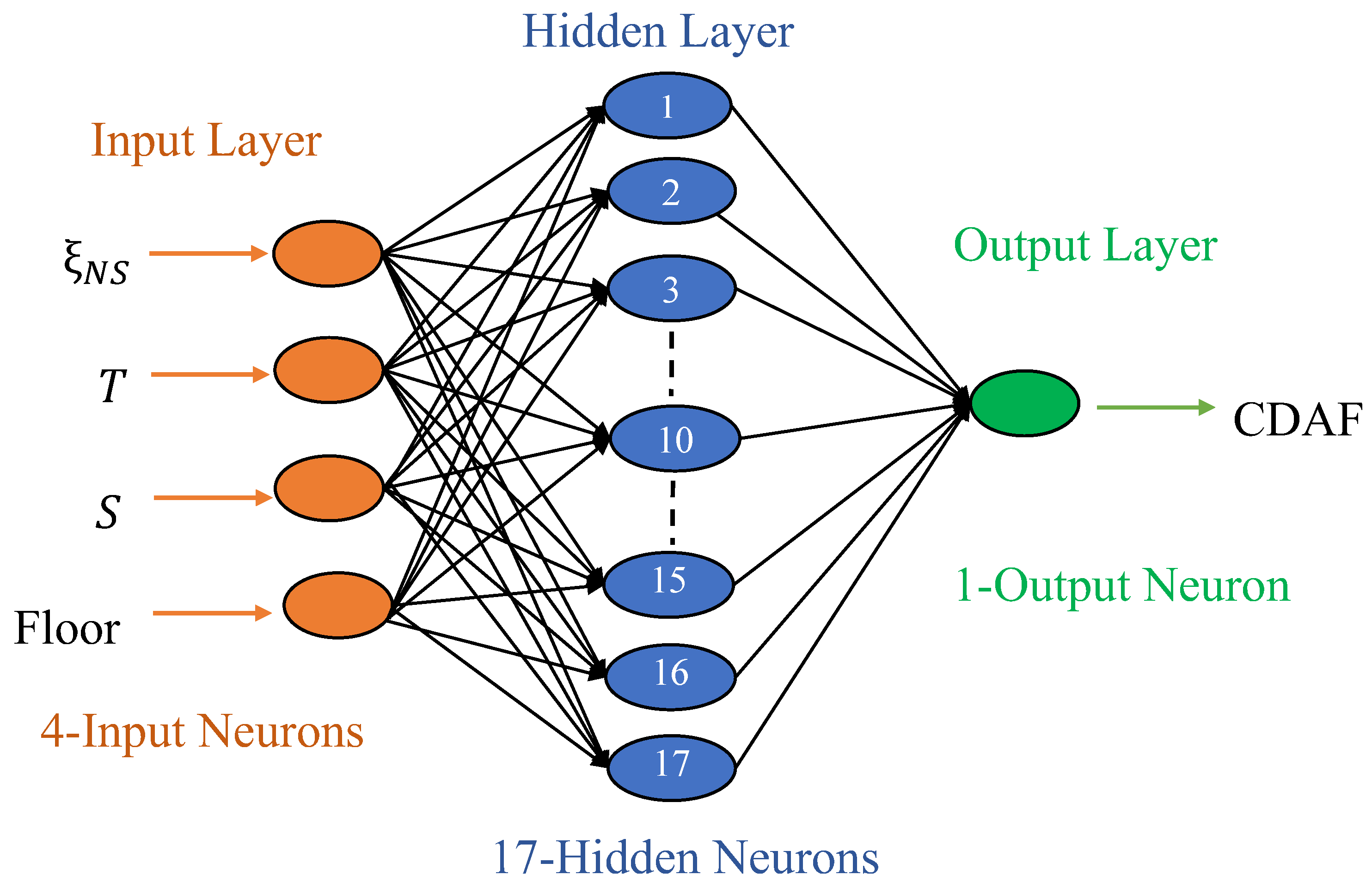
6. Artificial Neural Network (ANN) Model
6.1. Predictive Expression Using ANN Model
6.2. Validation of ANN-Based Predictive Expression
7. Summary and Conclusions
- The peaks observed in the floor response spectra correspond to the fundamental natural periods of the considered building models.
- The presence of mass irregularity at the lower story of the considered building models amplified the floor acceleration response at all floor levels for all soil types.
- Floor acceleration response increased in the irregular building by 26.1% and 10% at 1st and 5th floor levels for hard soil compared with the regular building.
- Floor spectral acceleration values increase with an increase in soil flexibility. In comparison with the hard soil, the floor spectral acceleration of a regular building’s 5th story increases by 32.4% in medium soil and by 41.3% in soft soil. Similarly, the floor spectral acceleration of an irregular building at the highest floor level (5th floor) increases by 29.2% in medium soil and 41.5% in soft soil compared with hard soil.
- Independent of building and soil type, it is found that the floor acceleration varies nonlinearly with building height. The values of the floor amplification factor increase with the building height and range from 1.08 to 3.85 for regular buildings and 1.53 to 4.55 for irregular buildings.
- The linear assumption in the code-based floor amplification formulation may lead to overestimation (first floor) and underestimation (second to fifth floor) of peak floor response demands.
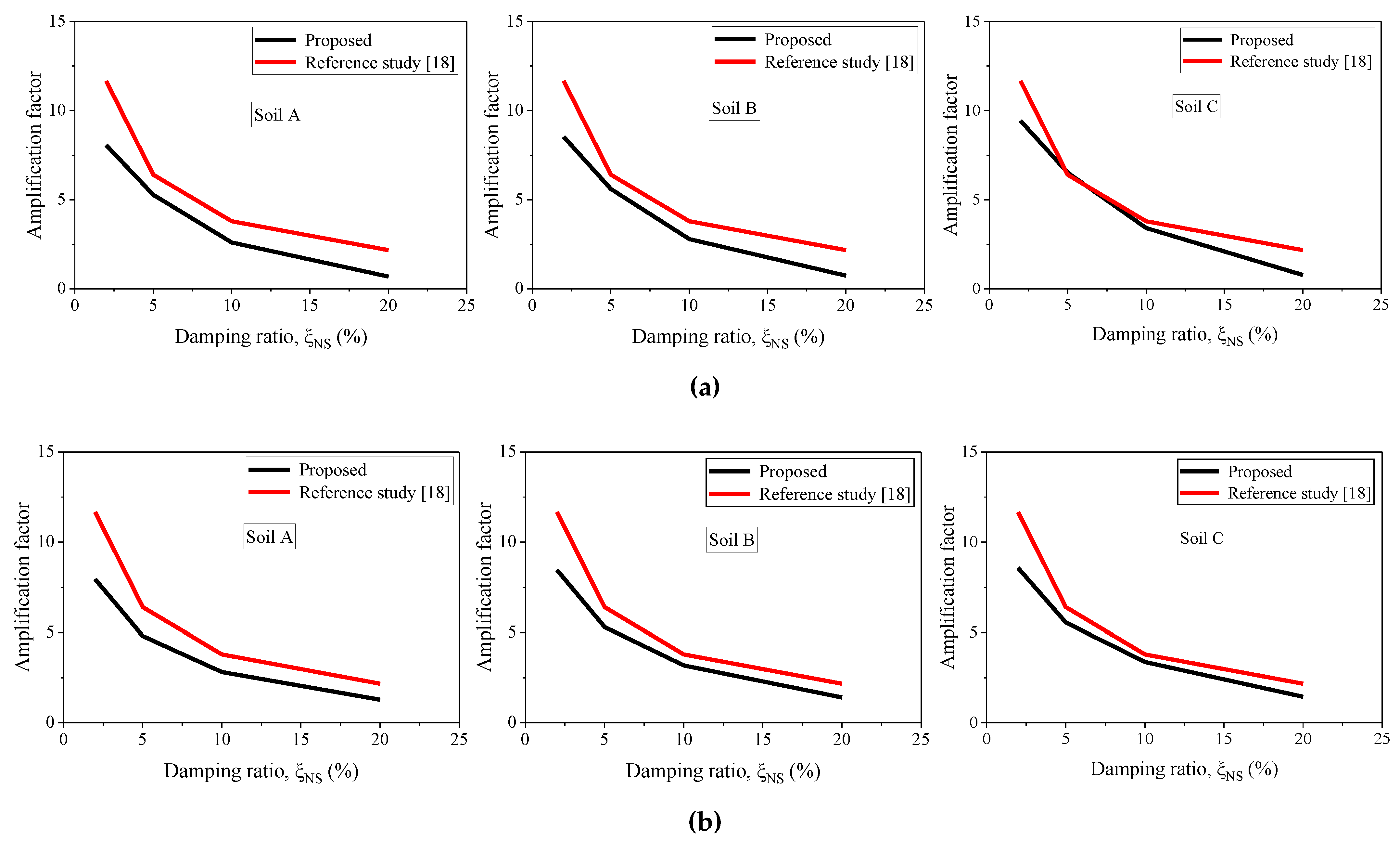
- The code definitions underestimate the peak component acceleration and dynamic amplification factors for all soil types.
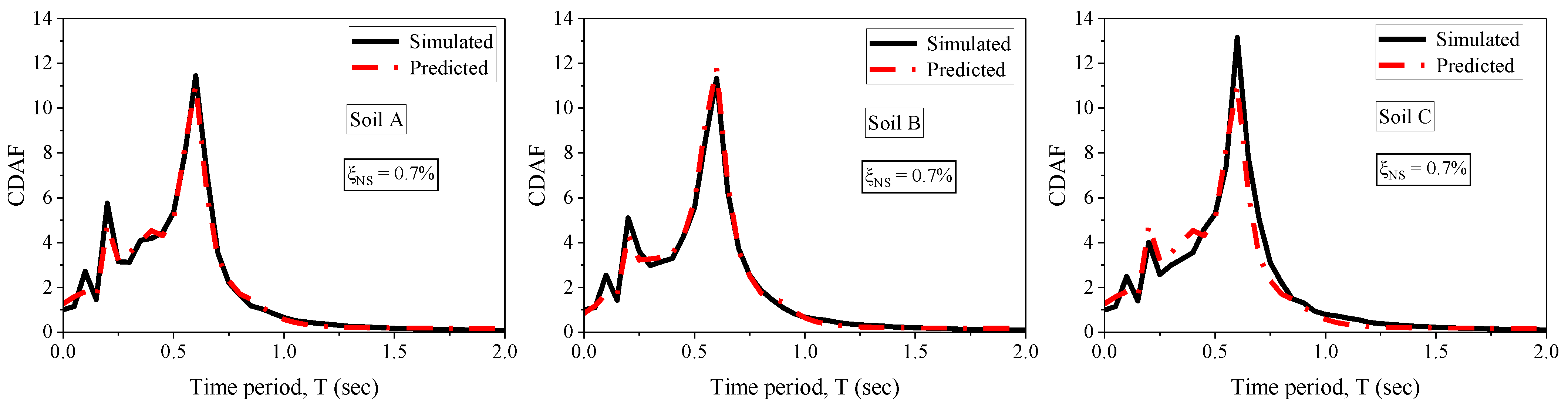
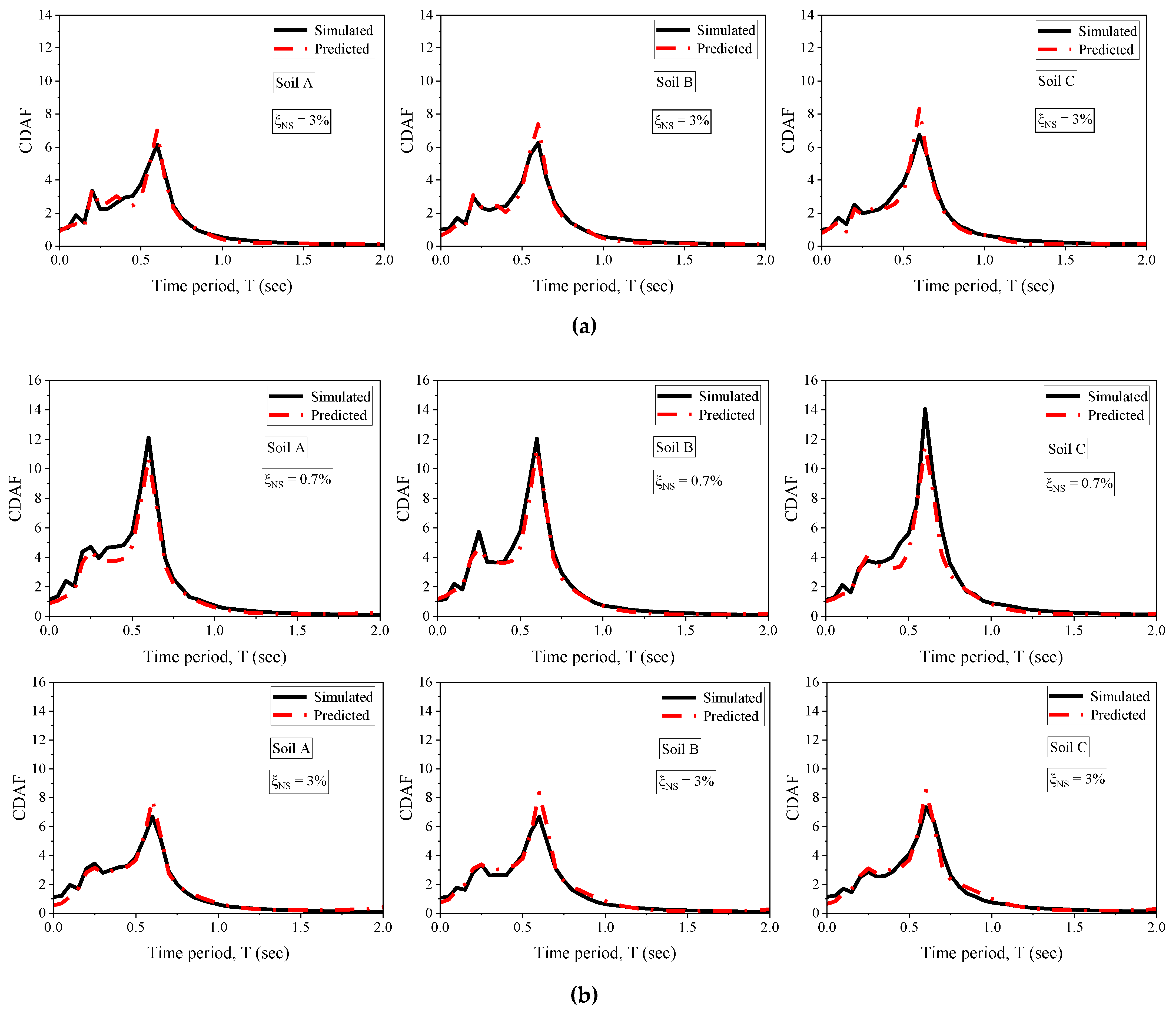
- The code definitions underestimate the CDAF for non-structural component periods closer to the vibration periods of the regular and irregular buildings for hard soil, while for medium and soft soil types, code definitions underestimate the CDAF for a non-structural component period closer to the fundamental vibration period of the building.
- The 4-17-1 ANN models developed in the present study can accurately predict the component dynamic amplification factors (CDAF) using various input parameters.
Author Contributions
Funding
Institutional Review Board Statement
Informed Consent Statement
Data Availability Statement
Conflicts of Interest
References
- Filiatrault, A.; Sullivan, T. Performance-based seismic design of nonstructural building components: The next frontier of earthquake engineering. Earthq. Eng. Eng. Vib. 2014, 13, 17–46. [Google Scholar] [CrossRef]
- Shang, Q.; Wang, T.; Li, J. Seismic fragility of flexible pipeline connections in a base isolated medical building. Earthq. Eng. Eng. Vib. 2019, 18, 903–916. [Google Scholar] [CrossRef]
- Di Sarno, L.; Magliulo, G.; D’Angela, D.; Cosenza, E. Experimental assessment of the seismic performance of hospital cabinets using shake table testing. Earthq. Eng. Struct. Dyn. 2019, 48, 103–123. [Google Scholar] [CrossRef] [Green Version]
- Anajafi, H.; Medina, R. Evaluation of ASCE 7 equations for designing acceleration-sensitive nonstructural components using data from instrumented buildings. Earthq. Eng. Struct. Dyn. 2018, 47, 1075–1094. [Google Scholar] [CrossRef]
- Suarez, L.E.; Singh, M.P. Floor response spectra with structure–equipment interaction effects by a mode synthesis approach. Earthq. Eng. Struct. Dyn. 1987, 15, 141–158. [Google Scholar] [CrossRef]
- Adam, C. Dynamics of Elastic–Plastic Shear Frames with Secondary Structures: Shake Table and Numerical Studies. Earthq. Eng. Struct. Dyn. 2001, 30, 257–277. [Google Scholar] [CrossRef]
- Menon, A.; Magenes, G. Definition of Seismic Input for Out-of-Plane Response of Masonry Walls: II. Formulation. J. Earthq. Eng. 2011, 15, 195–213. [Google Scholar] [CrossRef]
- Challagulla, S.P.; Bhargav, N.C.; Parimi, C. Evaluation of Damping Modification Factors for Floor Response Spectra via Machine Learning Model. In Structures; Elsevier: Amsterdam, The Netherlands, 2022; Volume 39, pp. 679–690. [Google Scholar]
- D’Angela, D.; Magliulo, G.; Cosenza, E. Seismic damage assessment of unanchored nonstructural components taking into account the building response. Struct. Saf. 2021, 93, 102126. [Google Scholar] [CrossRef]
- Vukobratović, V.; Fajfar, P. A method for the direct determination of approximate floor response spectra for SDOF inelastic structures. Bull. Earthq. Eng. 2015, 13, 1405–1424. [Google Scholar] [CrossRef]
- Jiang, W.; Li, B.; Xie, W.-C.; Pandey, M.D. Generate floor response spectra: Part 1. Direct spectra-to-spectra method. Nucl. Eng. Des. 2015, 293, 525–546. [Google Scholar] [CrossRef]
- Calvi, P.M.; Sullivan, T.J. Estimating floor spectra in multiple degree of freedom systems. Earthq. Struct. 2014, 7, 17–38. [Google Scholar] [CrossRef]
- Zhai, C.-H.; Zheng, Z.; Li, S.; Pan, X.; Xie, L.-L. Seismic response of nonstructural components considering the near-fault pulse-like ground motions. Earthq. Struct. 2016, 10, 1213–1232. [Google Scholar] [CrossRef]
- Petrone, C.; Magliulo, G.; Manfredi, G. Floor response spectra in RC frame structures designed according to Eurocode 8. Bull. Earthq. Eng. 2016, 14, 747–767. [Google Scholar] [CrossRef]
- Berto, L.; Bovo, M.; Rocca, I.; Saetta, A.; Savoia, M. Seismic safety of valuable non-structural elements in RC buildings: Floor Response Spectrum approaches. Eng. Struct. 2020, 205, 110081. [Google Scholar] [CrossRef]
- Landge, M.V.; Ingle, R.K. Comparative study of floor response spectra for regular and irregular buildings subjected to earthquake. Asian J. Civ. Eng. 2021, 22, 49–58. [Google Scholar] [CrossRef]
- Singh, M.P.; Suarez, L.E. Seismic response analysis of structure–equipment systems with non-classical damping effects. Earthq. Eng. Struct. Dyn. 1987, 15, 871–888. [Google Scholar] [CrossRef]
- Shang, Q.; Li, J.; Wang, T. Floor acceleration response spectra of elastic reinforced concrete frames. J. Build. Eng. 2022, 45, 103558. [Google Scholar] [CrossRef]
- Li, B.; Jiang, W.; Xie, W.-C.; Pandey, M.D. Generate floor response spectra, Part 2: Response spectra for equipment-structure resonance. Nucl. Eng. Des. 2015, 293, 547–560. [Google Scholar] [CrossRef]
- Dexter, A. Advances in characterization of soil structure. Soil Tillage Res. 1988, 11, 199–238. [Google Scholar] [CrossRef]
- Mercado, F.J.V.; Azizsoltani, H.; Gaxiola-Camacho, J.R.; Haldar, A. Seismic Reliability Evaluation of Structural Systems for Different Soil Conditions. Int. J. Geotech. Earthq. Eng. 2017, 8, 23–38. [Google Scholar] [CrossRef]
- Kumar, M.; Mishra, S.S. Study of seismic response characteristics of building frame models using shake table test and considering soil–structure interaction. Asian J. Civ. Eng. 2019, 20, 409–419. [Google Scholar] [CrossRef]
- Boulkhiout, R.; Messast, S. Effect of Soil on the Seismic Response of Structures Taking Into Consideration Soil-Structure Interaction. Int. J. Geotech. Earthq. Eng. 2020, 11, 72–90. [Google Scholar] [CrossRef]
- Hassan, A.; Pal, S. Effect of soil condition on seismic response of isolated base buildings. Int. J. Adv. Struct. Eng. 2018, 10, 249–261. [Google Scholar] [CrossRef] [Green Version]
- Jayalekshmi, B.R.; Chinmayi, H.K. Effect of soil stiffness on seismic response of reinforced concrete buildings with shear walls. Innov. Infrastruct. Solutions 2016, 1, 2. [Google Scholar] [CrossRef] [Green Version]
- Ceroni, F.; Sica, S.; Pecce, M.; Garofano, A. Effect of Soil-Structure Interaction on the Dynamic Behavior of Masonry and RC Buildings. In Proceedings of the 15th World Conference on Earthquake Engineering (WCEE), Lisbon, Portugal, 24–28 September 2012. [Google Scholar]
- Choi, Y.; Ju, H.; Jung, H.-J. Floor Response Spectrum of Nuclear Power Plant Structure Considering Soil-Structure Interaction. In Vibration Engineering for a Sustainable Future; Springer: Berlin/Heidelberg, Germany, 2021; pp. 161–166. [Google Scholar]
- Surana, M.; Singh, Y.; Lang, D.H. Effect of structural characteristics on damping modification factors for floor response spectra in RC buildings. Eng. Struct. 2021, 242, 112514. [Google Scholar] [CrossRef]
- Adam, C.; Furtmüller, T.; Moschen, L. Floor Response Spectra for Moderately Heavy Nonstructural Elements Attached to Ductile Frame Structures. In Computational Methods in Earthquake Engineering; Springer: Berlin/Heidelberg, Germany, 2013; pp. 69–89. [Google Scholar]
- Indian Standard (IS), IS 1893 (Part 1); Criteria for Earthquake Resistant Design of Structures, Part-1, General Provisions and Building. Sixth Revision. Bureau of Indian Standards: New Delhi, India, 2016.
- Indian Standard (IS), IS 875 (Part 2)–1987 (Reaffirmed 1997); Code of Practice for Design Loads (Other Than Earthquake) for Buildings and Structures, Part 2. Bureau of Indian Standards: New Delhi, India, 1998.
- SAP2000® Version 17; Integrated Software for Structural Analysis and Design, Computers and Structures, Inc.: Walnut Creek, CA, USA; New York, NY, USA, 2015.
- Surana, M.; Singh, Y.; Lang, D.H. Effect of irregular structural configuration on floor acceleration demand in hill-side buildings. Earthq. Eng. Struct. Dyn. 2018, 47, 2032–2054. [Google Scholar] [CrossRef]
- Biggs, J.M.; Rosset, J.M. Seismic Analysis of Equipment Mounted on a Massive Structure, Seismic Design for Nuclear Power Plants; Hansen, R.J., Ed.; Mass: Cambridge, UK, 1970. [Google Scholar]
- Bagheri, B.; Nivedita, K.A.; Firoozabad, E.S. Comparative Damage Assessment of Irregular Building Based on Static and Dynamic Analysis. Int. J. Civ. Struct. Eng. 2013, 3, 505. [Google Scholar]
- Senaldi, I.E.; Magenes, G.; Penna, A.; Galasco, A.; Rota, M. The Effect of Stiffened Floor and Roof Diaphragms on the Experimental Seismic Response of a Full-Scale Unreinforced Stone Masonry Building. J. Earthq. Eng. 2014, 18, 407–443. [Google Scholar] [CrossRef]
- PEER Ground Motion Database. Pacific Earthquake Engineering Research Center. University of California, Berkeley, CA, USA, 2013. Available online: http://ngawest2.berkeley.edu (accessed on 1 October 2022).
- American Society of Civil Engineers (ASCE). Minimum Design Loads and Associated Criteria for Buildings and Other Structures, ASCE 7-16; American Society of Civil Engineers: Reston, VA, USA, 2017. [Google Scholar]
- NEHRP Recommended Seismic Provisions for New Buildings and Other Structures (FEMA P-750); Federal Emergency Management Agency, Building Seismic Safety Council: Washington, DC, USA, 2009.
- Khy, K.; Chintanapakdee, C.; Wijeyewickrema, A.C. Application of Conditional Mean Spectrum in Nonlinear Response History Analysis of Tall Buildings on Soft Soil. Eng. J. 2019, 23, 135–150. [Google Scholar] [CrossRef]
- Al Atik, L.; Abrahamson, N. An Improved Method for Nonstationary Spectral Matching. Earthq. Spectra 2010, 26, 601–617. [Google Scholar] [CrossRef] [Green Version]
- Seismosoft. SeismoMatch—A Computer Program for Spectrum Matching of Earthquake Records, 2020. Available online: https://seismosoft.com/products/seismomatch/ (accessed on 1 October 2022).
- Eurocode 8: Design of Structures for Earthquake Resistance-Part 1: General Rules, Seismic Actions and Rules for Buildings; European Committee for Standardization: Brussels, Belgium, 2005.
- Chinese Standard 50011-2010; Code for Seismic Design of Buildings. Ministry of Housing and Urban-Rural Development: Beijing, China, 2010.
- Aragaw, L.F.; Calvi, P.M. Earthquake-Induced Floor Accelerations in Base-Rocking Wall Buildings. J. Earthq. Eng. 2021, 25, 941–969. [Google Scholar] [CrossRef]
- Flood, I.; Christophilos, P. Modeling construction processes using artificial neural networks. Autom. Constr. 1996, 4, 307–320. [Google Scholar] [CrossRef]
- Flood, I.; Kartam, N. Neural Networks in Civil Engineering. II: Systems and Application. J. Comput. Civ. Eng. 1994, 8, 149–162. [Google Scholar] [CrossRef]
- Jeng, D.S.; Cha, D.H.; Blumenstein, M. Application of Neural Network in Civil Engineering Problems. In Proceedings of the International Conference on Advances in the Internet, Processing, Systems and Interdisciplinary Research, Sveti Stefan, Montenegro, 5–11 October 2003. [Google Scholar]
- Shahin, M.A.; Jaksa, M.B.; Maier, H.R. Artificial Neural Network-Based Settlement Prediction Formula for Shallow Foundations on Granular Soils. Aust. Geomech. J. 2002, 37, 45–52. [Google Scholar]
- Challagulla, S.P.; Parimi, C.; Pradeep, S.; Farsangi, E. Estimation of dynamic design parameters for buildings with multiple sliding non-structural elements using machine learning. Int. J. Struct. Eng. 2021, 11, 147–172. [Google Scholar] [CrossRef]
- Challagulla, S.P.; Parimi, C.; Anmala, J. Prediction of Spectral Acceleration of a Light Structure with a Flexible Secondary System Using Artificial Neural Networks. Int. J. Struct. Eng. 2020, 10, 353–379. [Google Scholar] [CrossRef]
- Hornik, K.; Stinchcombe, M.; White, H. Multilayer feedforward networks are universal approximators. Neural Netw. 1989, 2, 359–366. [Google Scholar] [CrossRef]
- Acharyya, R.; Dey, A. Assessment of bearing capacity for strip footing located near sloping surface considering ANN model. Neural Comput. Appl. 2019, 31, 8087–8100. [Google Scholar] [CrossRef]
- Bhargav, N.C.; Challagulla, S.P.; Farsangi, E.N. Prediction Model for Significant Duration of Strong Motion in India. J. Appl. Sci. Eng. 2022, 26, 279–292. [Google Scholar]


| Earthquake | Year | Station | Mw | Rjb (km) | Vs30 (m/s) |
|---|---|---|---|---|---|
| Helena_ Montana-01 | 1935 | Carroll College | 6 | 2.07 | 593.35 |
| Helena_ Montana-02 | 1935 | Helena Fed Bldg | 6 | 2.09 | 551.82 |
| Kern County | 1952 | Pasadena, CIT Athenaeum | 7.36 | 122.65 | 415.13 |
| Kern County | 1952 | Santa Barbara Courthouse | 7.36 | 81.3 | 514.99 |
| Kern County | 1952 | Taft Lincoln School | 7.36 | 38.42 | 385.43 |
| Southern Calif | 1952 | San Luis Obispo | 6 | 73.35 | 493.5 |
| Parkfield | 1966 | Cholame, Shandon Array #12 | 6.19 | 17.64 | 408.93 |
| Parkfield | 1966 | San Luis Obispo | 6.19 | 63.34 | 493.5 |
| Parkfield | 1966 | Temblor pre-1969 | 6.19 | 15.96 | 527.92 |
| Borrego Mtn | 1968 | Pasadena, CIT Athenaeum | 6.63 | 207.14 | 415.13 |
| Borrego Mtn | 1968 | San Onofre, So Cal Edison | 6.63 | 129.11 | 442.88 |
| Earthquake | Year | Station | Mw | Rjb (km) | Vs30 (m/s) |
|---|---|---|---|---|---|
| Humbolt Bay | 1937 | Ferndale City Hall | 5.8 | 71.28 | 219.31 |
| Imperial Valley-01 | 1938 | El Centro Array #9 | 5 | 32.44 | 213.44 |
| Northwest Calif-01 | 1938 | Ferndale City Hall | 5.5 | 52.73 | 219.31 |
| Imperial Valley-02 | 1940 | El Centro Array #9 | 6.95 | 6.09 | 213.44 |
| Northwest Calif-02 | 1941 | Ferndale City Hall | 6.6 | 91.15 | 219.31 |
| Northern Calif-01 | 1941 | Ferndale City Hall | 6.4 | 44.52 | 219.31 |
| Borrego | 1942 | El Centro Array #9 | 6.5 | 56.88 | 213.44 |
| Imperial Valley-03 | 1951 | El Centro Array #9 | 5.6 | 24.58 | 213.44 |
| Northwest Calif-03 | 1951 | Ferndale City Hall | 5.8 | 53.73 | 219.31 |
| Kern County | 1952 | LA, Hollywood Stor FF | 7.36 | 114.62 | 316.46 |
| Northern Calif-02 | 1952 | Ferndale City Hall | 5.2 | 42.69 | 219.31 |
| Earthquake | Year | Station | Mw | Rjb (km) | Vs30 (m/s) |
|---|---|---|---|---|---|
| Imperial Valley-06 | 1979 | El Centro Array #3 | 6.53 | 10.79 | 162.94 |
| Imperial Valley-07 | 1979 | El Centro Array #3 | 5.01 | 14.54 | 162.94 |
| Coalinga-01 | 1983 | Parkfield, Cholame 2WA | 6.36 | 43.83 | 173.02 |
| Coalinga-01 | 1983 | Parkfield, Fault Zone 1 | 6.36 | 41.04 | 178.27 |
| Morgan Hill | 1984 | Foster City, APEEL 1 | 6.19 | 53.89 | 116.35 |
| Superstition Hills-02 | 1987 | Liquefaction Array | 6.54 | 23.85 | 179 |
| Superstition Hills-01 | 1987 | Liquefaction Array | 6.22 | 17.59 | 179 |
| Whittier Narrows-01 | 1987 | Carson, Water St | 5.99 | 26.3 | 160.58 |
| Loma Prieta | 1989 | Foster City, Menhaden Court | 6.93 | 45.42 | 126.4 |
| Loma Prieta | 1989 | Foster City, APEEL 1 | 6.93 | 43.77 | 116.35 |
| Loma Prieta | 1989 | APEEL 2, Redwood City | 6.93 | 43.06 | 133.11 |
| Regular Model | Irregular Model | |
|---|---|---|
| 1st mode | 0.603 | 0.612 |
| 2nd mode | 0.189 | 0.219 |
| 3rd mode | 0.104 | 0.130 |
| Mode | Regular Model | Irregular Model | ||
|---|---|---|---|---|
| 1st | 0.82 | 0 | 0.72 | 0 |
| 2nd | 0.93 | 0 | 0.94 | 0 |
| 3rd | 0.97 | 0 | 0.99 | 0 |
| 4th | 0.99 | 0 | 1.0 | 0 |
| 5th | 1.0 | 0.63 | 1.0 | 0.61 |
| 6th | 1.0 | 0.63 | 1.0 | 0.61 |
| 7th | 1.0 | 0.63 | 1.0 | 0.61 |
| 8th | 1.0 | 0.86 | 1.0 | 0.83 |
| 9th | 1.0 | 0.86 | 1.0 | 0.83 |
| 10th | 1.0 | 0.93 | 1.0 | 0.93 |
| 11th | 1.0 | 0.93 | 1.0 | 0.93 |
| 12th | 1.0 | 0.96 | 1.0 | 0.96 |
| Dataset | Regular Model | Irregular Model | ||
|---|---|---|---|---|
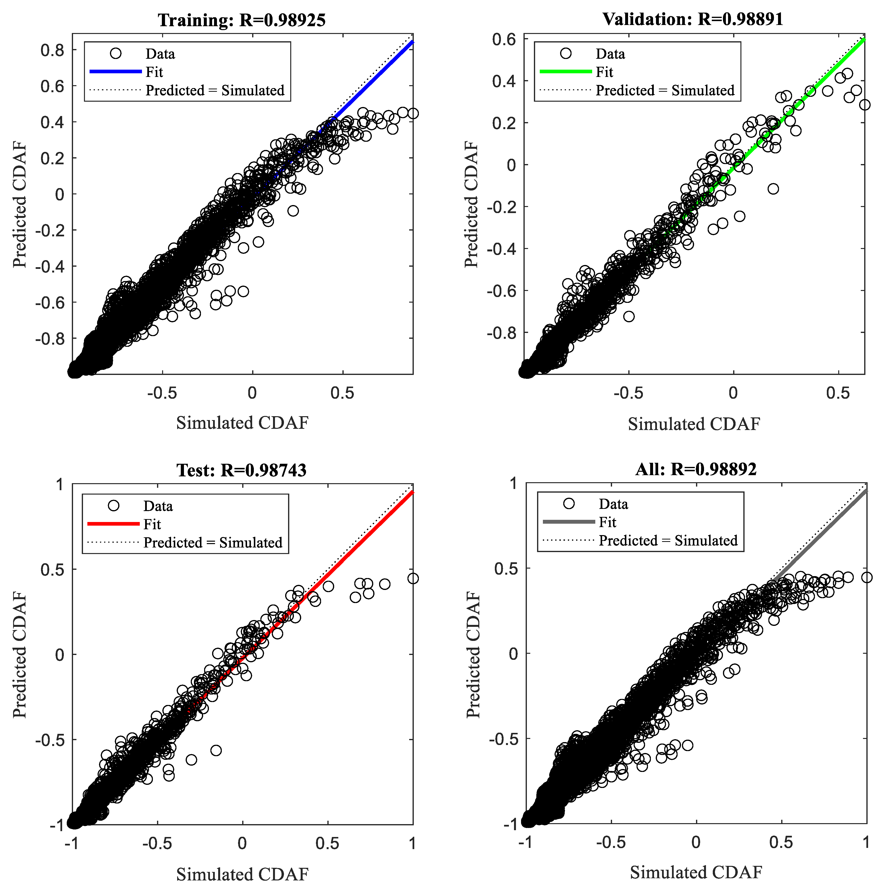
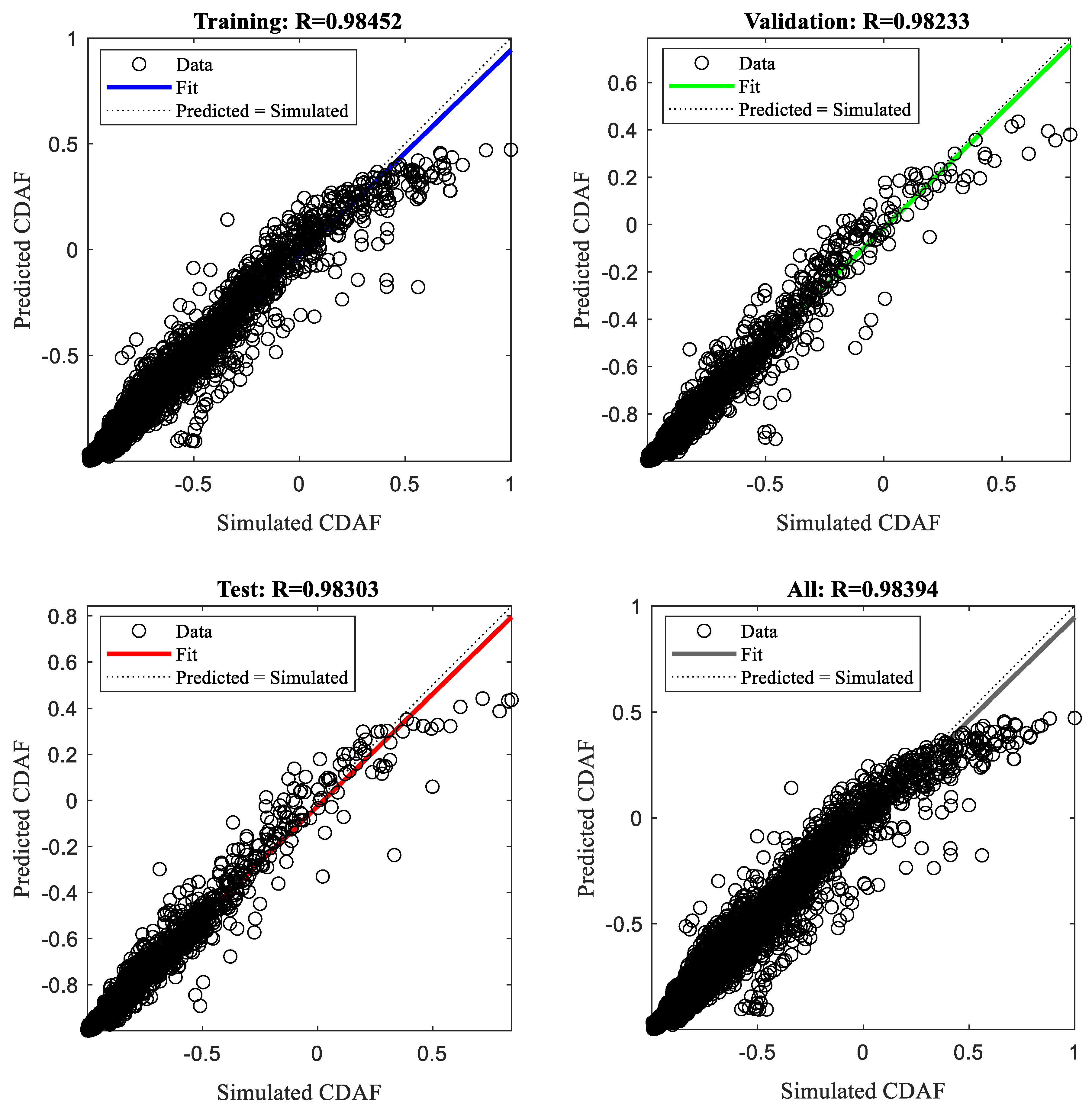
| Training | 0.989 | 0.00091 | 0.984 | 0.0012 |
| Testing | 0.987 | 0.00096 | 0.983 | 0.0019 |
| Hidden Neuron | Input-Hidden Weight | Hidden-Output Weight | Bias | ||||
|---|---|---|---|---|---|---|---|
| S | Floor | CDAF | Hidden | Output | |||
| 1 | −68.809 | −3.090 | 46.460 | −4.962 | −0.143 | −8.113 | 10.732 |
| 2 | 3.427 | 0.113 | −0.063 | −0.021 | −1.425 | 0.611 | |
| 3 | −68.642 | −6.979 | 11.368 | 0.189 | 0.053 | −34.320 | |
| 4 | 0.137 | 4.842 | 0.009 | 0.019 | −13.283 | 7.106 | |
| 5 | 22.380 | 0.396 | 8.460 | 1.107 | 0.130 | 11.461 | |
| 6 | −5.362 | −0.109 | 4.665 | −1.013 | 4.460 | −3.463 | |
| 7 | −32.567 | −1.630 | 28.505 | 27.228 | 0.044 | 25.297 | |
| 8 | −17.193 | −0.253 | 0.019 | −0.010 | 14.987 | −7.060 | |
| 9 | 17.085 | 0.202 | −0.018 | 0.015 | 15.110 | 7.019 | |
| 10 | 34.729 | 0.493 | 0.056 | −1.679 | 0.370 | 31.978 | |
| 11 | 5.423 | 0.078 | −4.727 | 1.190 | −8.203 | 4.012 | |
| 12 | −2.685 | 0.239 | −0.038 | 1.322 | −0.239 | −2.188 | |
| 13 | −5.118 | −0.085 | 4.431 | −1.058 | −12.737 | −3.639 | |
| 14 | 2.966 | 0.081 | 0.020 | 0.519 | 0.976 | 2.195 | |
| 15 | −46.845 | −43.367 | −0.059 | 0.496 | 0.078 | −60.467 | |
| 16 | −33.267 | −0.202 | −0.096 | −0.223 | −11.119 | −27.673 | |
| 17 | 30.736 | 0.220 | 0.099 | 0.261 | −11.738 | 25.571 | |
| Hidden Neuron | Input-Hidden Weight | Hidden-Output Weight | Bias | ||||
|---|---|---|---|---|---|---|---|
| S | Floor | CDAF | Hidden | Output | |||
| 1 | −1.823 | −7.929 | −0.136 | 0.233 | −2.726 | 4.917 | −3.109 |
| 2 | 1.926 | 13.893 | 0.032 | −0.192 | 1.251 | 3.018 | |
| 3 | −1.796 | 0.169 | 0.061 | −0.003 | 2.886 | 0.085 | |
| 4 | −5.367 | −0.440 | −6.494 | 2.704 | 0.118 | −1.311 | |
| 5 | −6.863 | 6.238 | 0.071 | −0.298 | 2.718 | 2.136 | |
| 6 | −6.562 | 5.712 | 0.081 | −0.301 | −2.957 | 1.885 | |
| 7 | 8.947 | −1.633 | 0.050 | 7.035 | −0.100 | −3.219 | |
| 8 | 20.749 | 2.468 | 0.057 | −0.922 | 0.482 | 20.907 | |
| 9 | 26.644 | 0.166 | 0.027 | 0.403 | −4.378 | 21.303 | |
| 10 | −14.638 | 0.262 | 0.007 | −0.020 | −8.095 | −5.555 | |
| 11 | 0.157 | 4.150 | 0.014 | −0.001 | 1.447 | 3.074 | |
| 12 | 7.773 | 0.332 | 11.839 | −7.140 | −0.103 | 13.698 | |
| 13 | −14.563 | 0.188 | 0.010 | −0.012 | 8.206 | −5.490 | |
| 14 | −36.300 | −1.397 | 0.126 | −3.951 | −0.289 | −26.922 | |
| 15 | 32.328 | 0.135 | 0.024 | 0.279 | 3.800 | 25.904 | |
| 16 | −0.177 | 0.404 | −0.010 | −0.005 | −14.903 | −0.063 | |
| 17 | 3.627 | −0.032 | 1.161 | −2.418 | −0.157 | −1.237 | |
| Input Parameters | Output Parameter | |||||
|---|---|---|---|---|---|---|
| (sec) | S | Floor | CDAF | |||
| Regular Model | Irregular Model | |||||
| Max | 2 | 20 | 2 | 5 | 20.545 | 19.504 |
| Min | 0 | 0.1 | 0 | 1 | 0.038 | 0.034 |
Disclaimer/Publisher’s Note: The statements, opinions and data contained in all publications are solely those of the individual author(s) and contributor(s) and not of MDPI and/or the editor(s). MDPI and/or the editor(s) disclaim responsibility for any injury to people or property resulting from any ideas, methods, instructions or products referred to in the content. |
© 2023 by the authors. Licensee MDPI, Basel, Switzerland. This article is an open access article distributed under the terms and conditions of the Creative Commons Attribution (CC BY) license (https://creativecommons.org/licenses/by/4.0/).
Share and Cite
Challagulla, S.P.; Kontoni, D.-P.N.; Suluguru, A.K.; Hossain, I.; Ramakrishna, U.; Jameel, M. Assessing the Seismic Demands on Non-Structural Components Attached to Reinforced Concrete Frames. Appl. Sci. 2023, 13, 1817. https://0-doi-org.brum.beds.ac.uk/10.3390/app13031817
Challagulla SP, Kontoni D-PN, Suluguru AK, Hossain I, Ramakrishna U, Jameel M. Assessing the Seismic Demands on Non-Structural Components Attached to Reinforced Concrete Frames. Applied Sciences. 2023; 13(3):1817. https://0-doi-org.brum.beds.ac.uk/10.3390/app13031817
Chicago/Turabian StyleChallagulla, Surya Prakash, Denise-Penelope N. Kontoni, Ashok Kumar Suluguru, Ismail Hossain, Uppari Ramakrishna, and Mohammed Jameel. 2023. "Assessing the Seismic Demands on Non-Structural Components Attached to Reinforced Concrete Frames" Applied Sciences 13, no. 3: 1817. https://0-doi-org.brum.beds.ac.uk/10.3390/app13031817