Adaptive λ-Control Strategy for Plug-In HEV Energy Management Using Fast Initial Multiplier Estimate

Abstract

This paper presents the application of the Lambda control strategy derived from Pontryagin’s Minimum Principle (PMP) for parallel PHEV. The proposed method has shown its efficiency for hybrid vehicles. It is here extended to the Plug-in hybrid vehicle case where reducing fuel consumption and ensuring optimal behavior of the state of charge of the battery are the specific, focused performance benchmarks. Offline PMP application requires the knowledge of the entire drive cycle to obtain optimal control, leading to the best engine energy consumption. Online, adapting this method requires a good estimation of the weighting parameter lambda value, which is not an obvious task. A fast initial estimation-based method is presented in this paper as a starting point for an adaptive L-control. The proposed method is then evaluated using standard driving cycles and compared with offline PMP results. Robustness study is also accomplished by testing method performances using mixed cycles.

1. Introduction

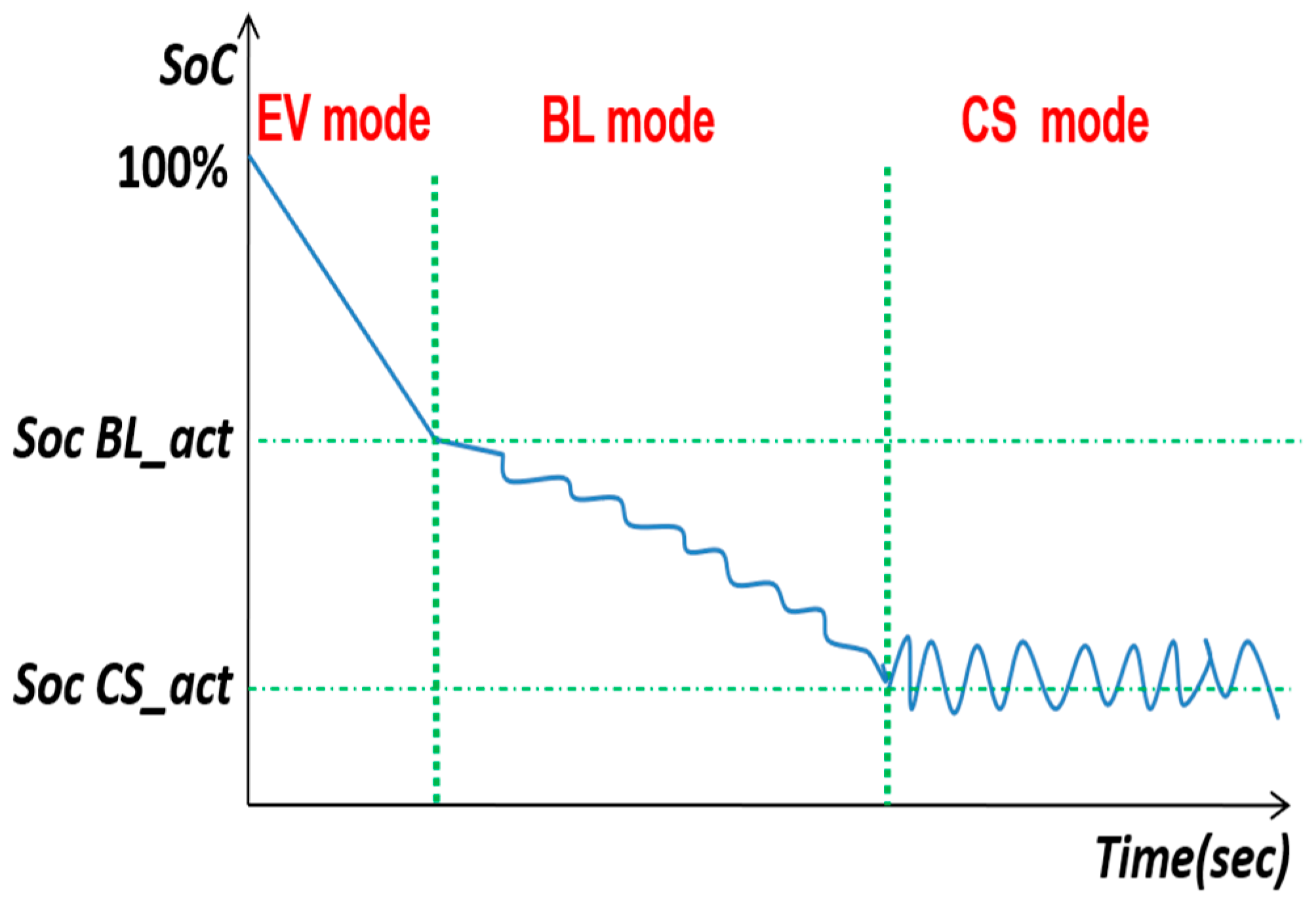
Hybridized vehicles are considered nowadays as an efficient technological solution to reduce gas emissions and non-renewable energy consumption. Plug-in hybrid vehicles are among the most studied alternatives to traditional vehicles as they allow the transfer of at least a part of the needed energy from fossil fuel to electricity. A plug-in hybrid electric vehicle (PHEV) is meanwhile a complex system as it combines two different energy sources: an internal combustion engine (ICE) with one or multiple electric motors (EM) powered by a rechargeable battery with important capacity providing zero gas emission (ZE) and an important all-electric-range (AER). The battery can be recharged via an external electrical outlet or powered either by the electric motor working as a generator during the deceleration and regenerative braking phase or by the internal combustion engine through a generator. During its use, the PHEV can operate on three modes generally depending on the state-of-charge (SoC) behavior which are:

-

Pure electric vehicle mode (EV), only the battery supplies the needed energy to the vehicle; the ICE is off.

-

Blended mode (BL): The ICE is on but supplies moderate power to allow the battery Soc depleting.

-

Charge-sustaining mode (CS): The ICE is the main energy source; the battery Soc is maintained at a given level.

These three modes are presented in Figure 1 [1].

Although the extensive use of EV mode results in simpler control and enhances electric energy consumption, studies and simulation results highlight the importance of blended mode in achieving energy savings in PHEV [2,3,4].

To ensure good battery management and optimal control, energy management strategy (EMS) algorithms are introduced to perform better power split between the two different sources of energy. They can be grouped in the literature into two categories: rule-based and optimization-based controllers. Rule-based algorithms consist of the implementation of a set of rules established from the PHEV operating modes (Figure 1) [1] while having expert knowledge of the system. While they are easy to implement, their establishment without prior knowledge of the road cycle does not present optimal results. A comparative study was introduced by [5,6] showing its limits for PHEV.

In [1], an application of a rule-based algorithm was introduced for parallel PHEV extended from the RL-based strategy for HEV. A parametric study was conducted pointing out the RL-based limitations and the variation effect of its dependent variables (SoC (state of charge) of the battery, LFS (Load Following Strategy) parameters) on fuel usage and initial trip battery level. The results show the combined importance of the selected phases of the PHEV (CD-CS), the battery Soc initial level, and the cycle driven in the efficiency of increasing the vehicle’s electric range and fuel economy.

On the other hand, optimization-based strategies are designed to achieve optimal control between the two energy sources via the minimization of a defined cost function in accordance with the required performances and the available parameters of the vehicle components. The optimization methods are grouped into two families. The first consists of global optimization controllers requiring a priori knowledge of the driving cycle (instantaneous speed profile), and a huge calculation capacity. The second uses real-time optimization controllers that rely on the real drive conditions without any prior cycle knowledge [2].

Several optimization strategies have been developed in the literature. The main algorithms are dynamic programming (DP) [7], equivalent fuel consumption minimization (ECMS) [8], simulated annealing (SA), genetic algorithms (GA), neural networks (NN) [9,10], slip mode control (SMC) [5], and model predictive control (MPC) [11,12]. Li in [13] uses PSO (Particle Swarm Optimization) algorithm to optimize rule-based control parameters for power-split Plug-in Hybrid Electric Vehicles. Haozhe in [14] presents a combination of fuzzy logic rules with a genetic algorithm to help save energy in the engine. Pu in [15] demonstrates an adaptive stochastic model predictive control strategy for a plug-in hybrid electric bus. A more detailed representation of energy management strategies has been introduced in [2,16].

Pontryagin’s Minimum Principle was extensively investigated and has proven its effectiveness in providing optimal fuel consumption for plug-in hybrid vehicles for the current decade. In [17,18], the map-based ECMS factor is adapted using a tan function for the required state of charge of the battery to be tracked according to the appropriate active mode, which manages the Chevrolet-volt engine on/off frequency. Each mode’s optimal control and speed are stored offline in tables and then controlled online using underestimated distance online. In [19], the authors provide a method to get lambda plots which present the LaGrange multiplier thresholds using dynamic programming to be applied after estimating its initial value on ECMS or PMP method on both series and parallel architectures. A comparison between EMS control using the PMP method with available drive pattern information or predictive driving information is introduced in [20] and applied to series-production vehicles where controllers have been developed to deal with uncertainty.

One of the most critical points of this method is the accurate calculation of the λ multiplier. Offline, when the driving cycle is entirely known, λ could be calculated precisely to achieve a targeted Soc at the end of the trip.

However, online this represents a real challenge as future use is never precisely known. This paper presents a derived method from optimization via the PMP algorithm commonly known as Lambda-control (λ-control). It aims to extend an λ-control strategy used for HEV in [21,22] and then developed here for a PHEV. Thus, the objective is to focus on the development of an efficient calculation of the initial value of the multiplier of the λ-control strategy, which is directly related to the evolution of the state of charge of the battery and the fuel flow. This is done by determining an estimated initial value calculated offline at the beginning of the trip yielding benchmark results, and subsequently correcting it online to ensure optimal control in real-time cases.

The article is structured as follows: Section 2 gives an overview of the modeling of the plug-in hybrid architecture: representation methods, driving cycle, simulation environments, and vehicle dynamics modeling. Then, in Section 3, the proposed λ-control algorithm is described, including both the offline and online calculation methods. Finally, strategy performances and robustness are tested using the appropriate tools implemented on MATLAB/Simulink with standardized driving cycles as inputs.

2. Plug-In Hybrid Architecture Modelling

The plug-in hybrid electric vehicle is a complex system whose energy management must be well-designed and evaluated to achieve the expected performance. The implementation of the global system optimal control is then necessary to ensure global control for effective management between the two energy sources. A systemic approach based on the modeling of the vehicle is considered where this multipart system is seen as a coupling of different subsystems interacting with each other and with the vehicle environment. Tools for modeling and representation are thus considered. Depending on the performance requirements and the objectives of the overall PHEV modeling, the direct model, also known as the “forward” model, makes it possible to determine the evolution of the dynamic system and the control strategy over time, deduced from the speed and acceleration as a function of the required torque.

Several representation methods have been introduced in the literature to facilitate modeling studies to design and control complex multi-physics systems, such as:

-

Bond graphs [23,24].

-

Energetic Macroscopic representation [25,26,27].

-

The mixed representation block diagram and graph bond is based on the representation of the subsystems in the form of block diagrams connected between them by energy variables.

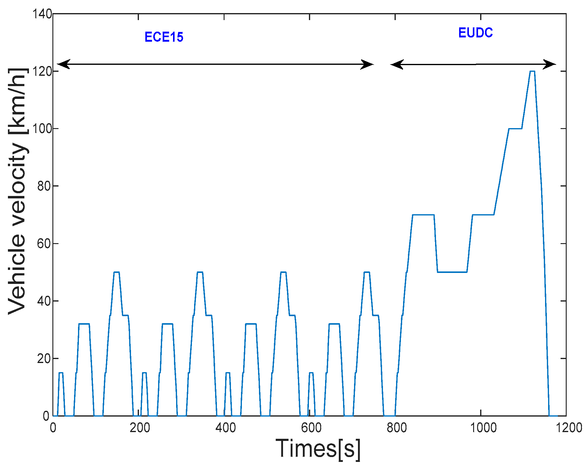
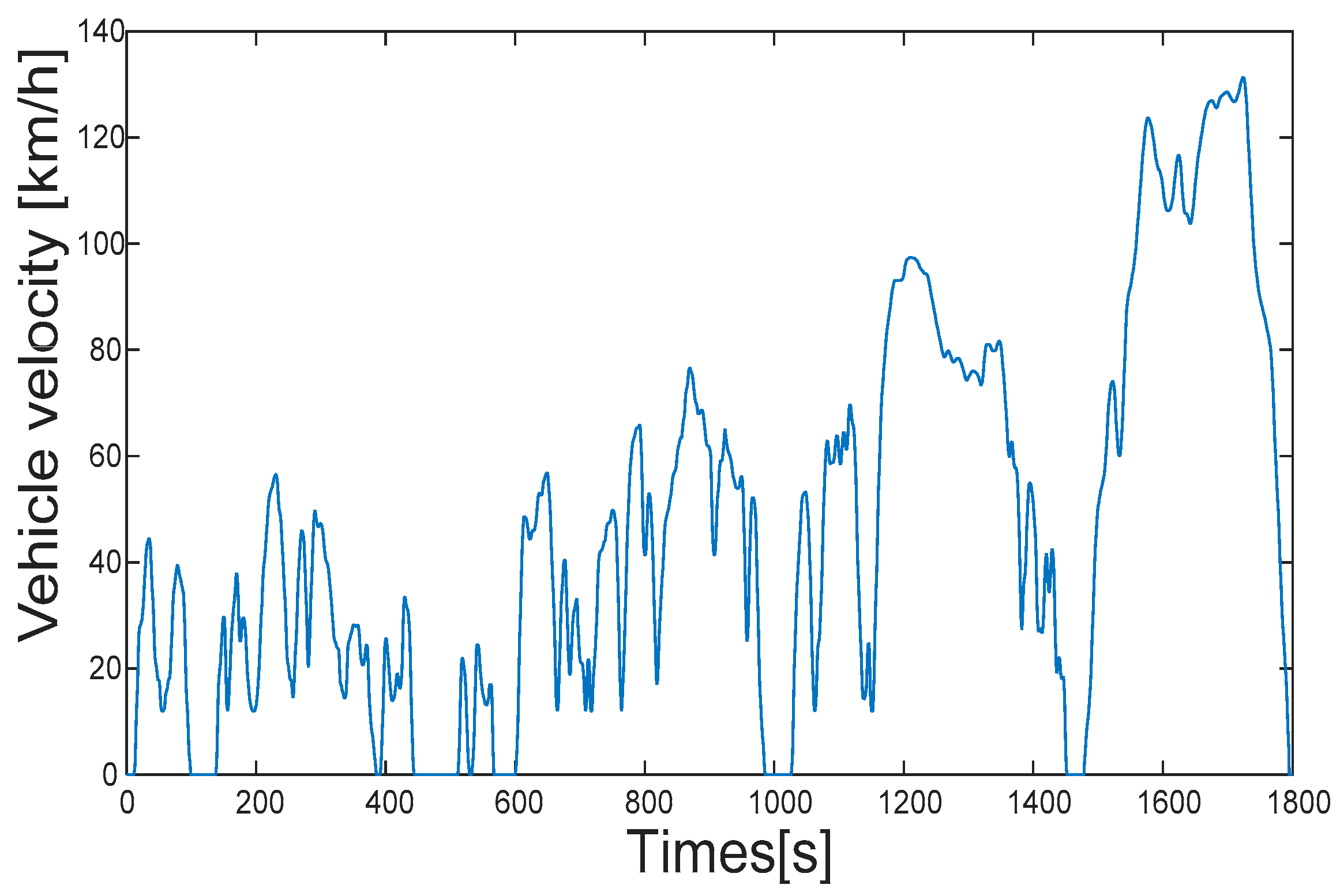
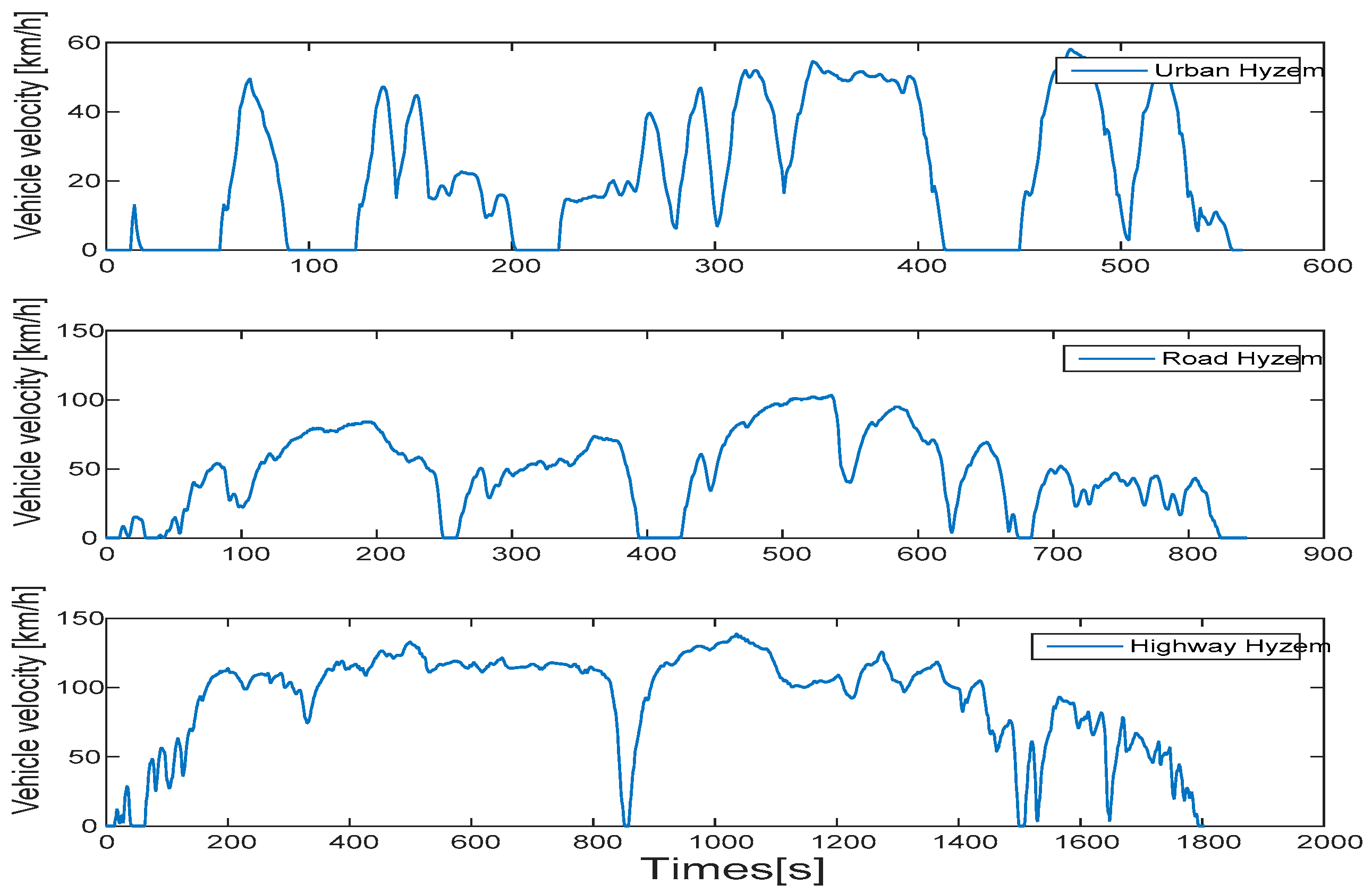
The implementation of an energy management strategy needs to be evaluated, and its performance assessed through the use of the driving cycle, which represents speed versus time and highly influences consumption and pollutant emissions. The most known in Europe are the standard cycles, such as the New European Driving Cycle (NEDC) (Figure 2, more recently replaced by WLTC (World Light vehicle Test Cycle) (Figure 3), and the real-life cycles based on experimental studies, such as Hyzem cycles (Figure 4).

There are many tools for simulating PHEVs’ behavior and validating their energy management. They depend on the type of approach and representations used for their modeling.

MATLAB/Simulink® seems to be one of the proper platforms to implement a mixed representation that allows various components models. VEHLIB, an open-source software developed by Gustave Eiffel University, uses this approach. Excepting the control, most of the models used for our PHEV come from this software [28,29,30].

In the context of technological developments, choosing the appropriate PHEV architecture is an important and cost-effective solution to achieve sustainable mobility and reduce the ecological footprint of the transport system. In this framework, the layout adopted is a parallel PHEV powertrain where a mechanical coupling is inserted between the ICE and the e-motor fitted in between the clutch and the gearbox. This link-up allows the thermal torque to be used in conjunction with the electric torque after the electrochemical energy conversion flow via the battery or separately. Thus, an all-electric self-driven mode can power the system, which meets the ecological requirements in urban areas.

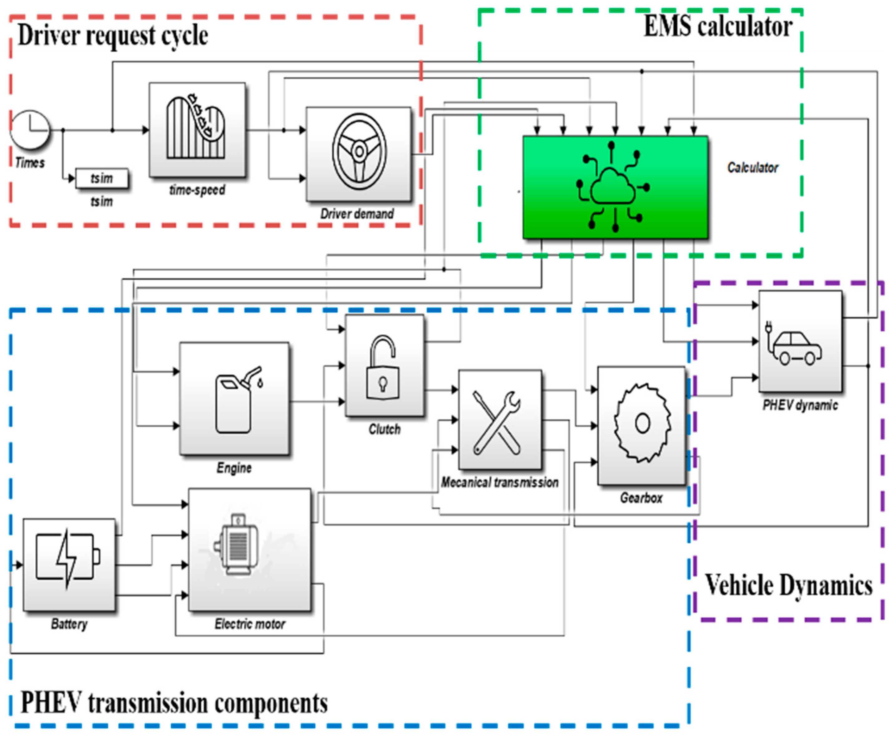
The global EMS-PHEV model consists of four main sub-blocks, as presented in Figure 5: the driver request cycle block, the EMS controller block, the PHEV transmission components block, and the vehicle Dynamics block.

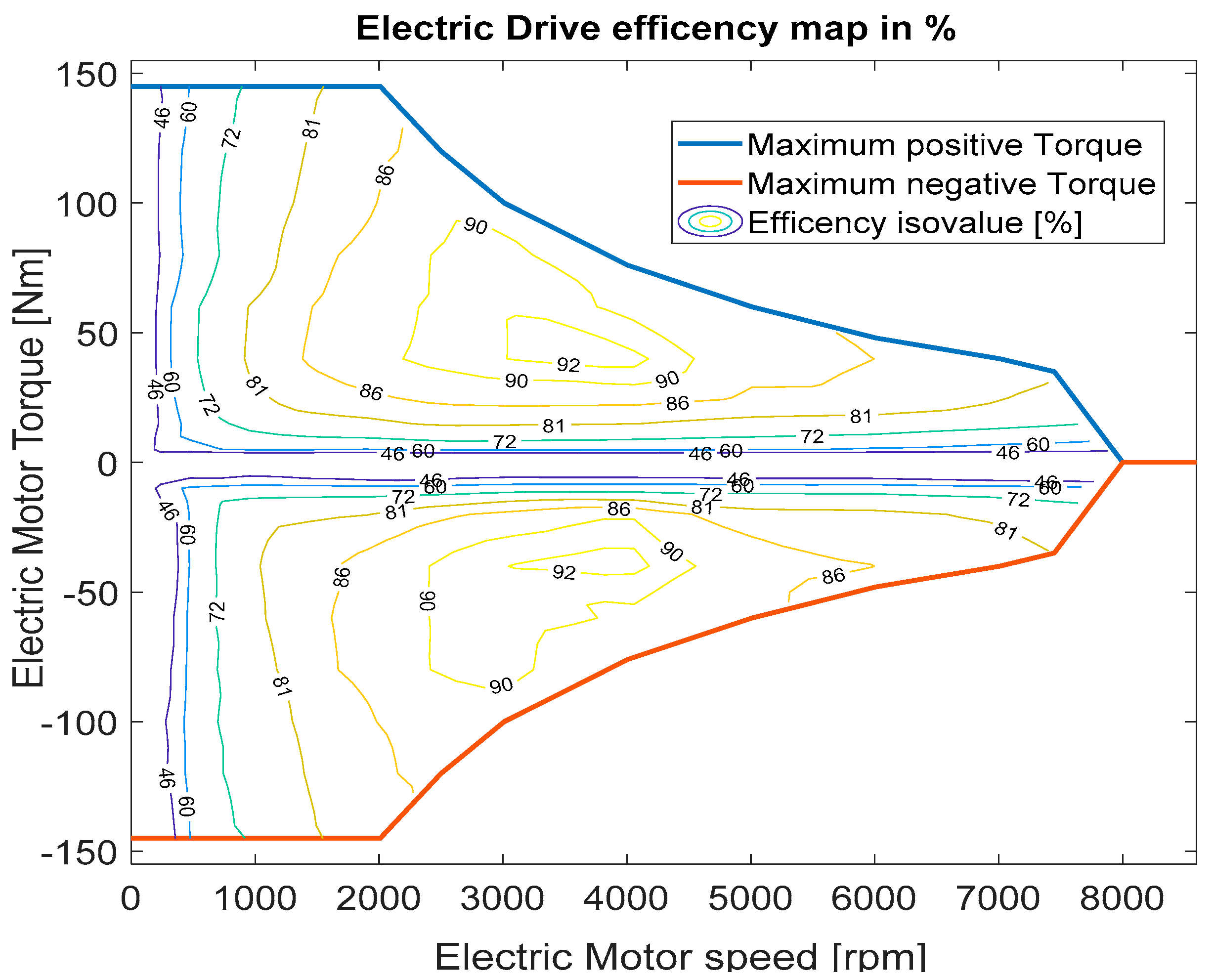
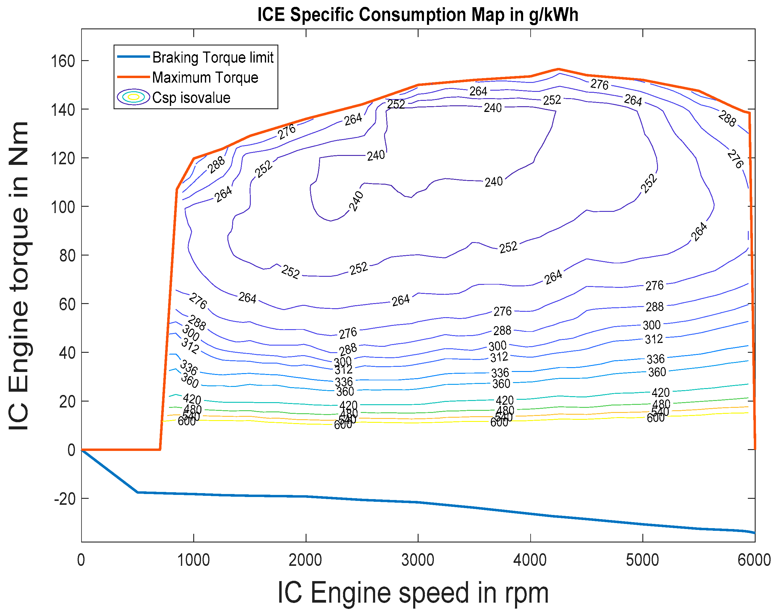
For the modeling of the powertrain, both the ICE engine and the electric drive parts that combines the electric motor with the converters are based initially on the efficiency operational maps (Figure 6 and Figure 7). In order to obtain mathematical models that could be easily used in our proposed EMS methods, these curves are approximated by polynomial expression. Equations (1) and (2) describe the fuel flow $S_{fuel}$ $(T_{ice}\left(k\right).W_{ice}$) and the required electric battery power $P_{BATT}$($T_{em}.W_{em}$) after operating the proposed interpolation.

$$\begin{gathered} S_{fuel}\left(k\right)=c_{1ice}.T_{ice}\left(k\right).W_{ice}{}^2+c_{2ce}.W_{ice}{}^2+c_{3ice}.T_{ice}{}^2\left(k\right).W_{ice}\left(k\right)+c_{4icec}.T_{ice}\left(k\right).W_{ice} \\ +c_{5ice}.W_{ice}\left(k\right).+c_{6ice}.T_{ice}{\left(k\right)}^2+c_{7ice}.T_{ice}\left(k\right)+c_{8ice} \end{gathered}$$

(1)

$$\begin{gathered} P_{BATT}\left(k\right)=T_{em}\left(k\right).W_{em}+c_{1em}.T_{em}\left(k\right).W_{em}{}^2+c_{2em}.W_{em}{}^2+c_{3em}.T_{em}{}^2\left(k\right).W_{em}\left(k\right)+c_{4em}.T_{em}\left(k\right).W_{em} \\ +c_{5em}.W_{em}\left(k\right).+c_{6em}.T_{em}{\left(k\right)}^2+c_{7em}.T_{em}\left(k\right)+c_{8em} \end{gathered}$$

(2)

where $T_{ice}$, $T_{em}$ are the engine and electric motor torques, $W_{ice}$, $W_{em}$ are the engine and electric motor speeds and $c_{Iice} \mathrm{and} c_{Iem}$ for $1\le I\le 8$ are the polynomial interpolation coefficients of the internal combustion engine and the electric motor.

The battery is a complex chemical device difficult to be mathematically described. In our case, it is modeled with a simple model of an equivalent electric circuit, which presents an open circuit voltage (OCV) connected in series with internal resistance, depending on the state of charge of the battery (SoC). As its evolution cannot be measured easily and accurately by sensors, SoC is defined as the ratio between the remaining capacity and its nominal capacity as presented in Equation (3) where $i_{batt}$ is the battery current, $C_n$ is the nominal capacity (Ah), and ${\eta }_F$ is the Faraday efficiency. The main battery characteristics are represented in

Table 1. Battery characteristics.

Component	Value (Unit)
Battery nominal capacity ($c_N$)	6.62 (Ah)
The terminal voltage of a cell	1.2 (V)
The terminal voltage of the battery pack	300 (V)
Number of cells in series Ns	40
Number of strings in parallel Np	4
Mass of a block	1.75 (kg)
Technology	NiMh

.

$$SoC\left(t\right)=SoC\left(t_0\right)-\frac{100{{\displaystyle \int }}_{t_0}^T{i}_{batt}\left(t\right){\eta }_F\left(sign i_{batt}\right)dt}{3600C_n}$$

(3)

$${\eta }_F\left(sign i_{batt}\right)=\{\begin{array}{c}0.95, i_{batt}<0\\ 1, i_{batt}\ge 0\end{array}$$

(4)

Furthermore, the vehicle is considered as an urban passenger car with a chassis, wheels, and the external environment (resistance forces) then, Equation (5) defines its longitudinal dynamics [22]. Here, the gearbox model considers a five-speed gearbox that can be changed instantly. The main vehicle parameters are depicted in

Table 2. Vehicle parameters.

Component	Value (Unit)
Unladen Vehicle mass (M)	1155 (kg)
Total Vehicle mass (Mv)	1479 (kg)
Aerodynamic drag coefficient (Cd)	0.35
The radius of the wheel (Rt)	0.29 (m)
Air density (Ρ)	1.18 (kg/m3)
The frontal area of the vehicle (Af)	1.92 (m2)
Internal combustion engine maximum power	86 (kW)
Motor maximum power	30 (kW)
Gearbox	Five ratios (k)

. The provided vehicle model and engine performance maps (Figure 7) allow for the calculation of speed and torque over time. Then the fuel consumption rate can be deduced using fuel flow projections $S_{fuel}$ $(T_{ice}\left(k\right).W_{ice}$).

$${\dot{w}}_{wh}\left(t\right)=\frac{1}{M_v{R}_t}\left(T_{wh}\left(t\right)-T_{res}\left(t\right)-T_{br}\left(\mathrm{t}\right)\right)$$

(5)

$$T_{res}=(m_{v}g(\sin \alpha +(a+b{v}^2)\cos \alpha )+\frac{1}{2}{\rho }_a{C}_d{A}_f{v}^2)R_t$$

(6)

where ${\dot{ w}}_{wh}$ is the angular acceleration of the wheels, $T_{wh}$ is the powertrain torque at the wheels (Nm) $(T_{wh}=R\left(k\right)(T_{ice}+\rho T_{em}))$, $T_{br}$ is the brake torque (Nm), $M_v$ is the total vehicle mass (kg) (covering the unladen vehicle mass (1155 kg), the mass of battery (280 kg), the engine (140 kg)) and the electric motor combined with the converters(59 kg)), R_t is wheel radius (m), $R\left(k\right)$ the gearbox speed ratio and $\rho$ reduction ratio between the electric and thermal motors, T_res is the resistant torque presented in Equation (6) [1], g is the gravity acceleration (m/s²), v is the vehicle velocity (m/s), A_f is the vehicle front area (m²), ρ is the air density (kg/m³), Cd is the aerodynamic drag coefficient, $\alpha$ is the road slope angle (rd) and a and b are rolling coefficients [1].

Moreover, the role of the supervision calculator EMS is to provide the system with the appropriate control of all the traction chain components: the electric torque, the thermal torque, the gearbox rate, and the brake command to the vehicle. For this purpose, the inputs are the required speed and torque, and the vehicle communicates accurate and timely status such as the estimated state of charge of the battery and the vehicle speed. To this extent, the calculator (ECU) must be carried out efficiently to well-coordinate the energy flow between the electric part and the thermal part according to the driver demand, preserving optimal control of the engine to improve engine energy efficiency. Furthermore, it has to select the proper active mode of the PHEV operations among the EV, the blended or the sustaining mode.

3. Proposed Optimization L-Control Strategy

3.1. Problem Formulation

This section provides an in-depth description of a PHEV’s studied energy management problem using an optimization-based control strategy. Considering the RL-based control strategy limitations, such as the need to have a good knowledge of the system operation and its sensitivity to several parameter fluctuations, the optimization-based EMS methods have more ability to track the optimum solution with its two basic options, i.e., global offline or online optimization (real-time optimization RT) [31].

Global offline optimization is most often achieved using dynamic programming, which is a time-consuming and thus cost-intensive numerical method or a faster method based on Pontryagin’s Minimum Principle (PMP) but with limitations in case of state variable saturation. These algorithms are used to evaluate the system performance, though the outcome is intended as a benchmark for the other real-time concepts and can be adapted to operate in this time scale [32].

For this purpose, the chosen algorithm for the EMS problem resolution in this work is the so-called λ-control which has been proven to ensure a good distribution of torques minimizing fuel consumption and pollutant emission. The λ-control is thus adapted from Pontryagin’s minimum principle in order to be reusable in real-driving conditions.

The basic idea is to approximate a one-time variable known as the Lagrange multiplier, on which depends a function H designated as the Hamiltonian, which is defined as a relation of the criterion to be minimized J, generally function of the control variable U, the system state variable x(t) as well as the multiplier λ. This function H has to be minimized by choosing the appropriate control variable U, yielding thus to a near-optimal solution. Appendix B presents more details about Pontryagin’s minimum principle (PMP) [32].

In this context, the aim of the strategy is:

-

To ensure optimal control achieving the minimum of the criterion chosen (see below).

-

To guarantee good PHEV-SoC battery management

-

To respect the drive-train components’ energy constraints.

-

To attain the transition from charge depleting mode (CD) to charge sustaining (CS) if the SoC reaches its minimum discharge limit value in order to keep it around there based on rule-based determined control; (If SoC reaches a predefined threshold, then, a certain selected mode is active).

To tackle this optimization problem according to the λ-control concept, a set of EMS steps must be identified in terms of the state variable to be controlled, the criteria that should be minimized, the control variable, and the constraints to be respected.

3.1.1. Identification of the State Variable

In order to manage well the electric energy storage system during the optimization process according to the PHEV mode of operations, the state of energy of the battery is the chosen state variable to be controlled. Its equation is as follows [32] where the $P_{BATT}$ is the delivered battery power:

$$X\left(t\right)=SoE\left(t\right)=SoE\left(t_0\right)-{{\displaystyle \int }}_{t_0}^t{P}_{BATT}dt$$

(7)

3.1.2. The Choice of the Criteria to Be Minimized

As the primary criteria to be evaluated is fuel consumption, the criteria providing the optimal solution is the specific fuel flow loss throughout the road cycle as expressed in Equation (8). For simplification and data provision, gas emissions are not considered in our case study. As the specific consumed fuel level depends on the internal combustion engine torque, this latter $T_{ice}$ is the control command yielding the best power split between the cross-over sources.

$$J={{\displaystyle \sum }}_0^{N-1}{\dot{S}}_{fuel} T_e$$

(8)

While considering efficiency and fuel consumption as the optimization criteria, some EMS could lead to intensive use of the battery. Therefore, in order to prolong battery lifetime, battery aging could be considered as the optimization criterion as depicted in [33] or one among the criteria of a multiobjective optimization [34]. This may be relevant in future studies as the proposed method could adapt to this issue.

3.1.3. Constraints

The developed approach must respect physical constraints basically related to the main powertrain components. Figure 6 illustrates the maximal and minimal electric motor torque ($T_{em}max$, $T_{em}min$) and maximal and minimal electric speed ($W_{em}\mathit{max}, W_{em}min$). Figure 7 presents the maximal, minimal and optimal engine torque ($T_{ice}\mathit{max}, T_{ice}\mathit{min}, T_{ice}opt$) as well as maximal and minimal engine speed $W_{ice}\mathit{max}, W_{ice}\mathit{min}.$

When the required vehicle power is negative (during the regenerative braking phase), it is assumed here that the energy recovery is only limited by the electric motor and the SoC charge acceptance (more precisely, the maximum negative battery current). In some studies [35], the sharing of electrical and mechanical braking according to the dynamical vehicle behavior is detailed. This could be introduced in the upcoming work in order to obtain more realistic results; however it is not in the scope of this article.

Furthermore, the battery constraints have bound the minimum and maximum current limitations as well as the minimum and maximum voltage as stated in Equations (9) and (10). These are considered to be the charging (I_batt < 0) and discharging (I_batt > 0) characteristics of the battery, which are reflected in its modeling.

$$I_{batt}min<I_{batt}<I_{batt}max$$

(9)

$$U_{batt}min<U_{batt}<U_{batt}max$$

(10)

On the other hand, a very significant concern of power monitoring is to control the electric energy storage system variation. In typical cases, this is carried out according to the active operating mode of the PHEV over the covered time path. In charge-depleting mode, the state of charge decreases up to a predefined limit ($So{C}_L$) to toggle then to the charge sustaining mode where the state of charge has to be maintained within this limit to the end of the trip operating as a conventionnel hybrid vehicle or plug into a socket. Equation (11) writes down the battery constraints to be respected in accordance with the state of energy variation ∆SOE in either CD or CS mode.

$${\displaystyle \sum }_{i=0}^{N-1}{P}_{batt}=\Delta SOE$$

(11)

3.1.4. Application of the λ-Control in EMS Problem

For the selected parameters, the Hamiltonian to be minimized can be expressed in Equation (12):

$$H\left(X\left(t\right),U\left(t\right), \lambda \left(t\right),t\right)={\dot{S}}_{fuel}\left(U\left(t\right),t\right)+\lambda \left(t\right)P_{BATT}$$

(12)

The first optimality condition applied to this case study at each point of time leads to Equations (13) and (14).

$$\frac{\partial H\left(k\right)}{\partial \lambda \left(k\right)}=SoE\left(k+1\right)$$

(13)

$$\frac{\partial H\left(k\right)}{\partial SoE\left(k\right)}=-\lambda \left(k+1\right)$$

(14)

Equation (14) referred to as the adjoint equation conducts to searching the initial unique lambda value that leads to the desired SoE over the considered time frame under the assumption that the state of charge of that battery doesn’t have a direct impact on the battery power before reaching its limits [32].

Furthermore, as the driving conditions are considered to be known in the global optimization approach, and the parameter λ has a direct impact on the Soc variation of the battery, the optimal control problem resides in finding the initial unique lambda value that leads to the desired SoE over the considered time frame.

For these purposes, the optimal control problem is answered with two sub-solutions verifying Equation (15) which are:

-

Off-line: resolute using the dichotomy principle based on the variation of the desired soc at the end of the trip as a function of $\lambda \left(0\right)$.

-

Online: Lagrange multiplier estimation: using the initial calculated value on offline mode under a cycle reference to be estimated later continuously or periodically using a closed-loop block for real-time driving conditions.

$$\Delta So{E}_{req} =f \left(\lambda \left(0\right)\right)$$

(15)

3.1.5. Determination of the Optimal Thermal Torque

The third optimality condition aims to find the optimal command vector $T_{ice}opt$ that can minimize the Hamiltonian H. In [21,22], the optimal thermal torque is solved for the charge-sustaining case study. If the initial value of the multiplier is considered to be known $\lambda \left(0\right)$, the application of the optimality conditions leads to the Equations (16)–(18). Since both the fuel rate and the power loss curves are approximated, implementing Equations (1) and (2) in the Hamiltonian Equations (17) and (18) leads to the expression of the optimal engine torque value that minimizes every single time the Hamiltonian H as it is defined in Equation (19) [22].

$$\frac{\partial H\left(k\right)}{\partial T_{ice}}=0$$

(16)

$${\frac{\partial H\left(k\right)}{\partial T_{ice}{}^2}}^2\ge 0$$

(17)

$$\frac{\partial H\left(k\right)}{\partial T_{ice}}=\frac{\partial S_{fuel}\left(k\right)+\lambda \left(0\right)P_{BATT}\left(k\right)}{\partial T_{ice}}$$

(18)

$$T_{ice}opt=\frac{A\left(k\right)\lambda \left(0\right)+C\left(k\right)}{B\left(k\right)\lambda \left(0\right)+D\left(k\right)}$$

(19)

where $A(k$), $C(k$), $B\left(k\right)$ and $D(k$) are functions of $W_{ice}\left(k\right)$ and the polynomial interpolation coefficients of the internal combustion engine and electric motor $c_{Iice} \mathrm{and} c_{Iem}$ for $1\le I\le 8$(Expressions are given in the Appendix A).

3.2. Offline Calculation Solution: λ(0)

The goal is to apply the dichotomy method to find the co-state $\lambda \left(0\right)$ providing an optimal solution that minimizes the fuel usage and best power split on the blended mode.

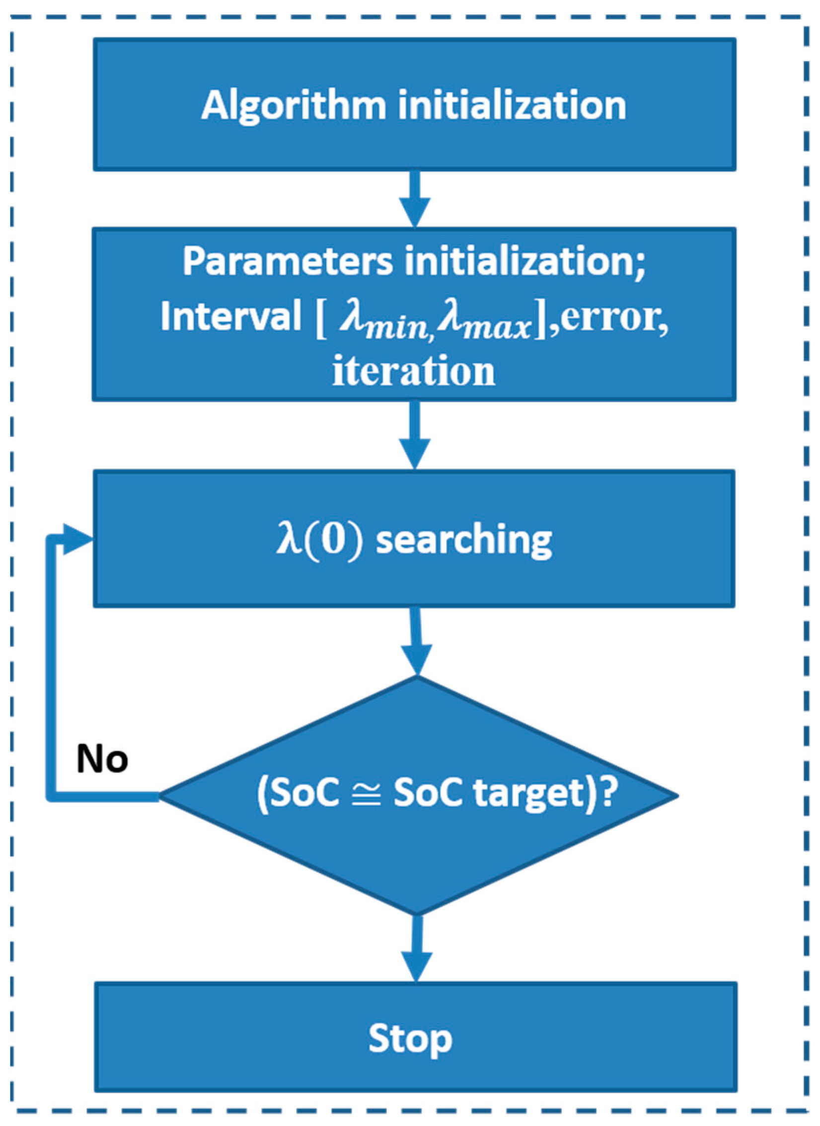
For this purpose, the proposed assumption is that for a given cycle, each value of λ(0) leads to a final state of charge in offline mode. In this framework, the optimal control is sought that leads to a minimum value of fuel consumption in order to reach a predefined minimum discharge value of 30% using a fully charged pack at the beginning. Figure 8 shows the proposed scheme of an offline L-Control calculation by the bisection method. To apply the bisection method, sets of steps have to be defined as the primary initialization parameters. In that case, λ(0) is selected to be included between [${\lambda }_{min},{\lambda }_{max}$]. Since the expected lambda value must satisfy an optimal control in blended mode, both boundaries fulfill the desired lambda values in electric-only mode and sustaining mode for an initial fully charged battery. As a consequence, the minimum lambda value ${\lambda }_{min},$ is set at the value where the system performs in all-electric mode throughout the journey. Whereas, to recall, in sustaining mode, the battery must support its state of charge within a pre-established band where the initial value must be balanced with the final value reached by the end of the trip, then the maximum value ${\lambda }_{max}$ is determined from the dichotomy technique for a zero Soc battery balance variation. On the other hand, the number of iterations, as well as the error, need to be deliberated in order to satisfy the trade-off between producing less fuel and reaching the desired SoE variation Equation (15).

For the sake of completeness, the obtained unique value of λ(0) in offline mode is introduced into the Hamiltonian algorithm using a prior known cycle as a benchmark to deliver the optimal control of the engine and the electric motor control according to Equation (12).

3.3. Online Calculation Solution: LaGrange Multiplier

As in real-time conditions, the drive pattern is considered to be not known. The aim is to estimate the lambda value in a continuous manner yielding to the near-optimal control of the combustion engine that makes the best energy saving according to pre-defined desired SoE variation.

3.3.1. Determination of the Estimated Initial Lambda Value: LaGrange Estimator

As mentioned above, the EMS problem should be resolved considering the constraint related to SoE variation of the battery ($\Delta So{E}_{req}$) during the trip cycle presented in Equation (11).

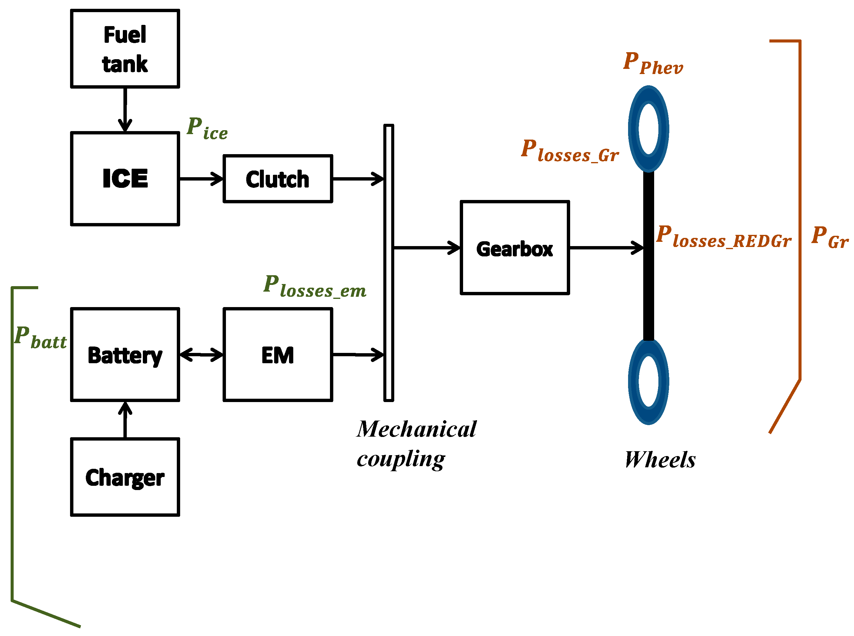
Figure 9 indicates the input/output power energy balance of a plug-in hybrid vehicle in a parallel configuration, and it is detailed in the following equations:

$$P_{batt}-P_{losses\_em}+P_{ice}=P_{Gr}$$

(20)

On the other hand,

$$P_{Gr}=P_{Phev}+P_{losses\_Gr}+P_{losses\_REDGr}$$

(21)

where $P_{batt}$ is the battery power, $P_{losses\_em}$ is the electrical losses power, $P_{Gr}$ is the Gearbox resultant power, $P_{ice}$ is the internal combustion engine power, $P_{VEH}$ is the plug-in hybrid electric vehicle power on the wheels, $P_{losses\_BV}$ are the Gearbox power losses and $P_{losses\_REDGr }$ is the reduction gear power losses.

Considering the powers expressions explained in Appendix A, Equation (11) presenting the state of energy variation is then depicted in Equation (22) in the function of the rolling conditions, the optimal engine torque, the engine speed, and both the gearbox and differential efficiency ratios.

$${\displaystyle \sum }_{i=0}^N{P}_{batt}={\displaystyle \sum }_{i=0}^N\left(T_{wh }{W}_{wh}\gamma \right)-{\displaystyle \sum }_{i=0}^N\left(T_{ice}opt W_{ice}\right){\alpha }_{ELEC}{}^{-S\left(i\right)}$$

(22)

$$\gamma ={\alpha }_{REDGr}{}^{-S\left(i\right)}{\alpha }_{Gr}{}^{-S\left(i\right)}$$

(23)

where, $T_{wh }$ is the powertrain torque at the wheels, $W_{wh}$ is the powertrain speed at the wheels, ${\alpha }_{ELEC}$ is the mean electrical efficiency ratio, ${\alpha }_{REDGr}$ is the differential reduction efficiency ratio, and ${\alpha }_{Gr}$ is the gearbox efficiency ratio.

Using Equations (11), (19), and (22), the resulting initial estimated lambda value is then as displayed in Equation (24).

$$\check{{\lambda }_{in{i}_{estimated}}\left(i\right)}=\frac{({{\displaystyle \sum }}_{i=0}^{N}C\left(i\right) W_{ice}\left(I\right){\alpha }_{ELEC}{}^{-s\left(i\right)}-{{\displaystyle \sum }}_{i=0}^N\left(T_{wh }{W}_{wh}\gamma D\left(i\right)\right))N+abs\left(\Delta SoE\right){{\displaystyle \sum }}_{i=0}^{N}D\left(i\right)}{({{\displaystyle \sum }}_{i=0}^{N}A\left(i\right) W_{ice}\left(i\right){\alpha }_{ELEC}{}^{-\mathrm{s}\left(\mathrm{i}\right)}-{{\displaystyle \sum }}_{i=0}^N(T_{wh }{W}_{wh}\gamma B\left(i\right){\alpha }_{ELEC}{}^{-s\left(i\right)}))N-abs\left(\Delta SoE\right){{\displaystyle \sum }}_{i=0}^{N}B\left(i\right) }$$

(24)

where S(i) is the sign of the power supplied by the gearbox, the electric motor and the gearbox to the wheels (S(i) = 1: propulsion, S(i) = −1: braking).

3.3.2. Adaptative λ-Control

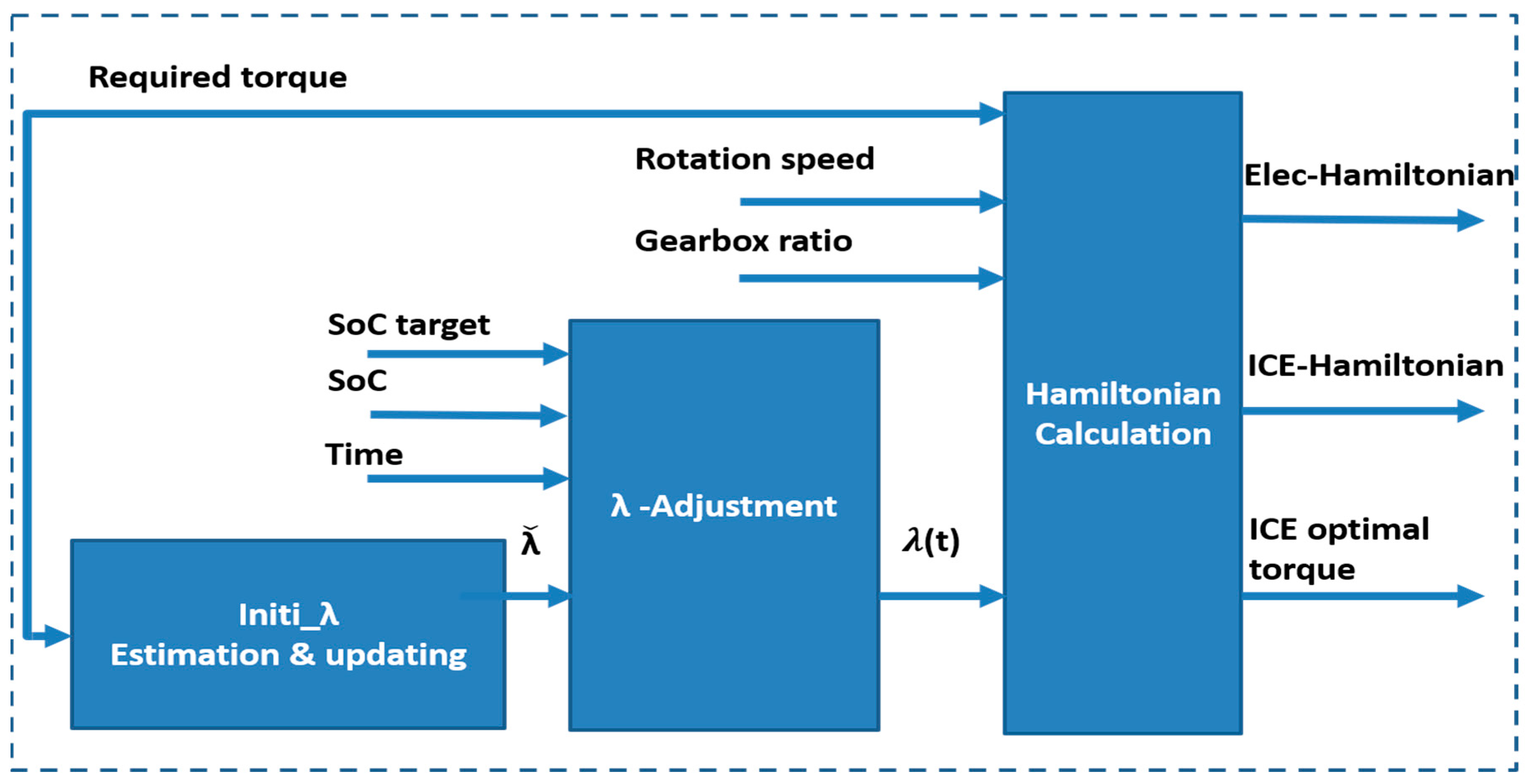
Operating with an open-loop structure usually leads, in the context of real-time control, to uncontrolled battery depletion, especially when the drive cycle is not known. For this reason, closed-loop control is prescribed. Figure 10 illustrates the proposed model of an efficient-adaptive lambda control in online computing. The principal inputs are the required vehicle torque, the required speed ($T_{wh }$, $W_{wh }$), the gearbox ratio, and the calculated lambda value estimated over the time-covered cycle in which the Hamiltonian function depends. The feedforward loop is then added to adjust this forecasted latter to further ensure that the evolution of the battery SoC does not deviate from the initial deployed required target while the driver is performing the journey. The proposed settlement is inspired by the similar controllers used in [36] for the various HEV powertrain architectures and also adopted in [22,32,37,38] to deal with parallel HEV for the EMS online optimization problem. It has been then extended in this article to resolve battery management of the different PHEV modes of operations.

Hence, a PI controller is implemented to correct the error between the SoC of the battery and the targeted SoC. In that case, the new calculated tuning factor λ over the time-variation is set in Equation (25). The required SoC of the battery $So{C}_{required}\left(d\left(t\right), \alpha , \beta \right)$ is a distance-dependent function where $\alpha$ and $\beta$ are parametric coordinates that differ according to the initial SoC of the battery and the final desired SoC value and the nature of the driving model that is involved. Here, the proposed desired SoC is a linear profile scheme that can be presented as a time or distance-based travel pattern.

On the other hand, the studies conducted in [39] revealed that the addition of the PID controller might cause occasional deviations in the expected performances regarding the tracking of the requested SoC of the battery by the time-current SoC and consequently on the engine optimal control. Therefore, the initial estimated value of lambda needs to be updated over time, as was mentioned in [32,38] according to the periodic update $N_{\lambda }$ parameter.

$$\lambda \left(t\right)={\lambda }_{in{i}_{estimated}}+K_P\left(SO{C}_{required}\left(d\left(t\right), \alpha , \beta \right)-SOC\left(t\right)\right)+K_I({\displaystyle \int }SO{C}_{required}\left(t, \alpha , \beta \right)-SoC\left(t\right)$$

(25)

To assess the process, it is then crucial to select these indicators properly. The latter are selected either through trial and error or through algorithmic optimization [24]. To this extent, ref. [40] adopted Equation (26) if SoC gets to its maximum value to justify the horizon parameter in the case of optimization using the model predictive control MPC. By determining the relevant initial estimated and updated lambda value, it is possible to calculate the Hamiltonian function and thus deliver the system with economic electrical and thermal control.

$$K_P\le \frac{\lambda \left(0\right)}{\left|So{C}_{required}-So{C}_{max}\right|}$$

(26)

4. Simulation Results and Discussion

The Global EMS parallel-PHEV model simulation is conducted using MATLAB/Simulink, as depicted in Figure 2, where the proposed EMS calculators are implemented. To test the latter efficiency, the driver demand is assumed under several consecutive NEDC cycles when the electric power supply system is initially fully laden.

Here, the total amount of test distance is 10,932 km for both Offline and online calculator calculations. As λ-control is also cycle-dependent, NEDC results can be interrupted easily compared with the proposed RL- based strategy in [1].

4.1. Offline Results

To confirm the proposed controller in the offline calculation, the search interval for the Lagrange multiplier is bounded to within the following two maximum and minimum values ${\lambda }_{min}$ = 5 × 10⁻⁵ and ${\lambda }_{max}$= 7.0114 × 10⁻⁵.

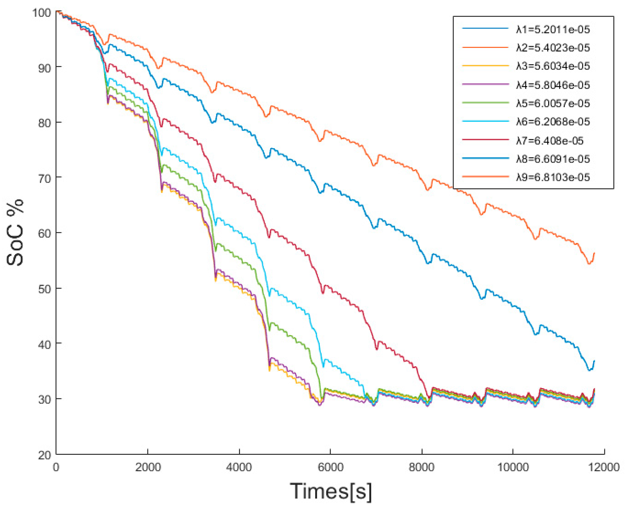
Before setting the primary initialization parameters of the bisection method, the trial-and-error method was applied to the global PHEV model in order to ensure the existence of the desired co-state and to confirm the choice of the boundary search interval. Figure 11 illustrates the state of the charge of the battery variation according to λ-Control parameters iteration in the offline calculation.

It reveals that the searched multiplier meeting the above hypothesis can be localized between the two parameters ${\lambda }_7$ and ${\lambda }_8$ for a fuel consumption rate of less than or equal to 1.95 L per 100 km.

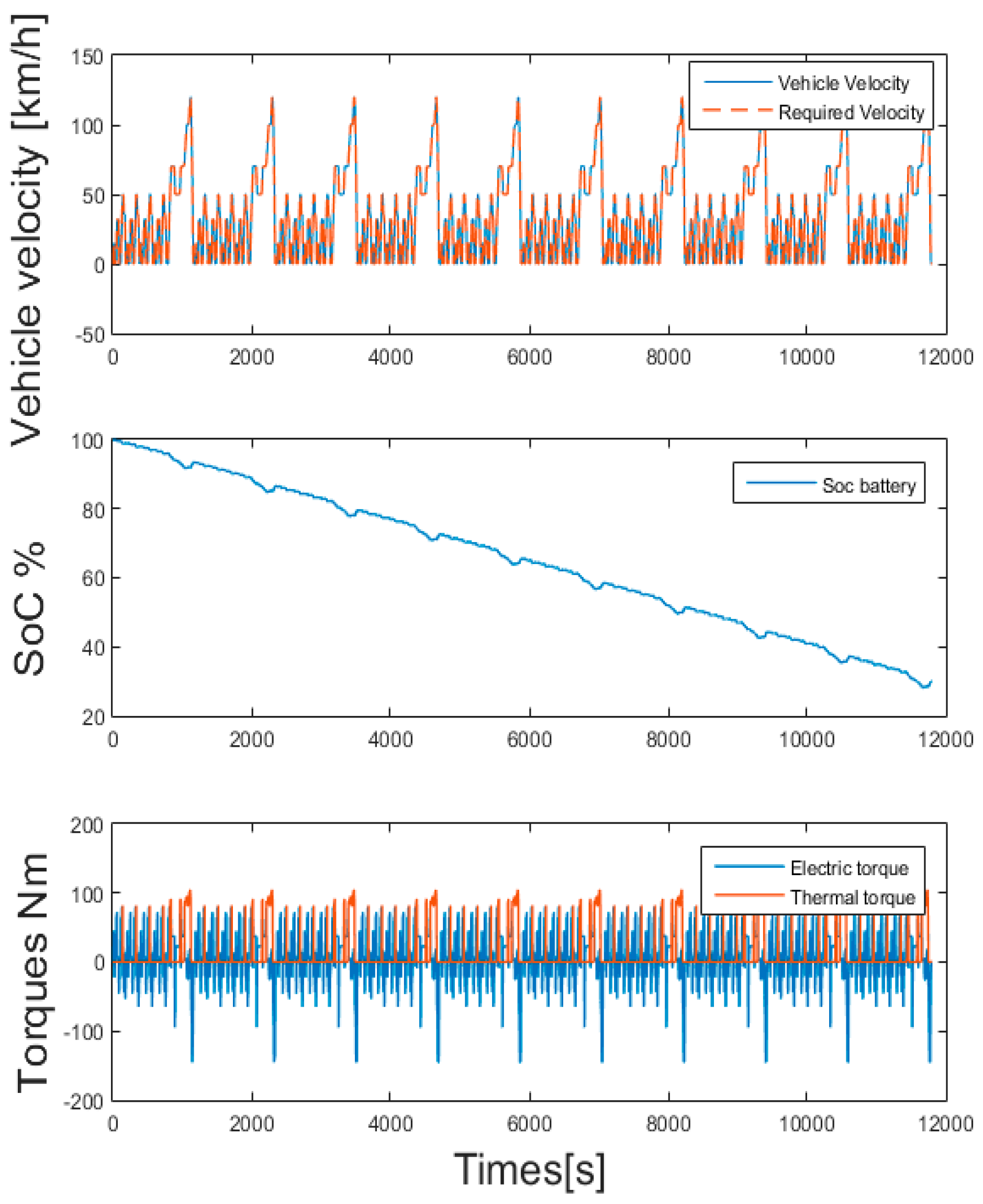
The co-state search problem λ(0) is solved after 25 iterations with an allowable ΔSoE tolerance error of 0.05 and a 0.1 s sampling period. After running through iterations, the found value λ(0) for ten consecutive NEDC driving cycles is equal to 6.5505 × 10⁻⁵. Thus, it is assumed to be the most effective value leading to optimal control results (in terms of fuel consumption) in blended mode with the target SoC performance of around 30% at the end of the trip. The resulting value is then fed into the system to test its evolution as well as the SoC variation and the use of the fuel rate. Figure 12 represents the vehicle velocity, the required vehicle velocity, the state of charge, and ICE and EM torques for the proposed offline λ-control algorithm for PHEV using the Bisection Method on the blended mode.

It proves good speed tracking and good SoC battery management over the journey. The third curve below presents the distributed energy flow of the thermal (red) and electric parts (blue). The system favors the use of the ICE in high energy demand to delay the earlier complete discharge of the battery and reach its required SoC value towards the end of the drive pattern. Only the electric motor supplies the negative power demand and allows the energy storage system to recharge during deceleration and braking phases.

It has been mentioned that throughout the system performance test, it is necessary to make a well-balanced compromise between the required set objectives. In this case, it can be assumed that the obtained λ(0) value assisted the system in improving the fuel economy rate to 1.86 L per 100 km for a final SoC found at the end of the trip close to the set target SoC balance value −70.02% $\left(\Delta SoC=So{C}_{final}-So{C}_{initial}\right)$.

4.2. Online Results

This section aims at validating the effectiveness of the proposed online controller mentioned above. The objective is to test the achievement of results as close as possible to those obtained offline, considered as reference solutions since in real-time, the driver behavior is not known.

The resulting initial estimated ${\lambda }_{in{i}_{estimated}}\left(0\right)$ value is equal to 5.0825 × 10⁻⁵ for a required SoE balance ΔSoE 70% of around 5338.368 Wh. The self-selected parametric coordinates of the required SoC to be tracked giving a final SoC of about 30% for an electric energy storage system with a full initial charge are (α = −0.0059 and β = 100).

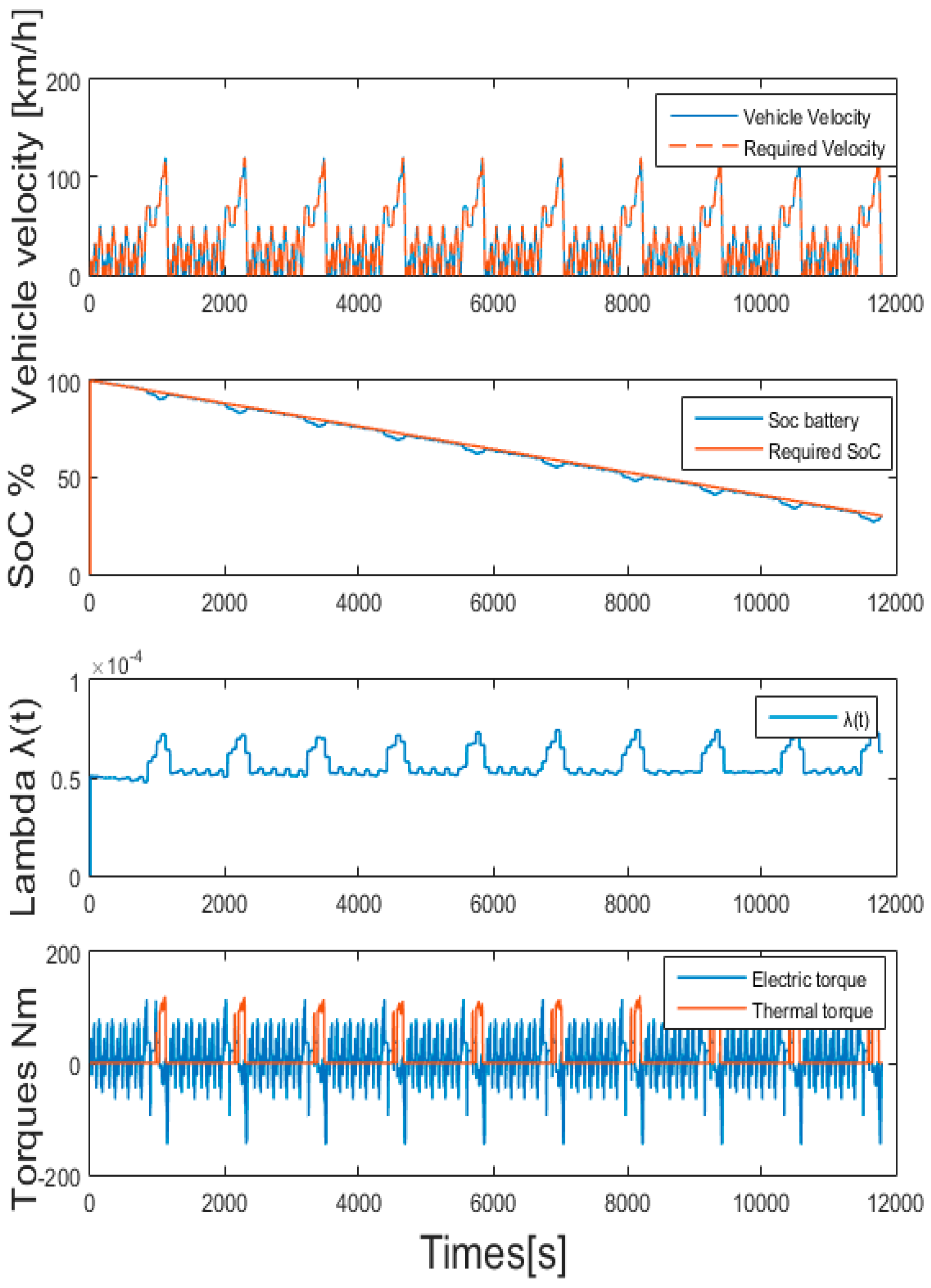
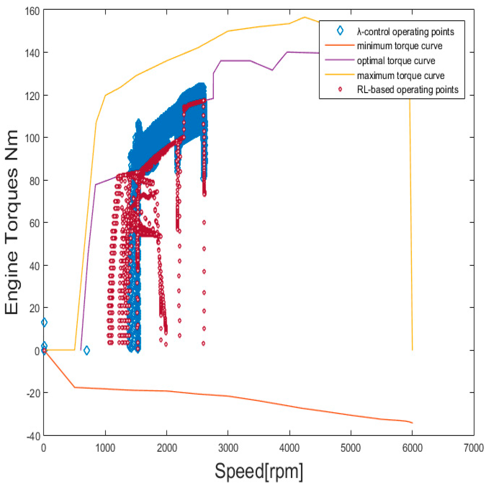
Figure 13 depicts the vehicle velocity, the required vehicle velocity, the state of charge, the required SoC, the multiplier variation, and ICE and EM torques for the proposed online λ-control algorithm for PHEV in the blended mode. Figure 14 presents the resulting ICE operating points within its optimal, maximum, and minimum torque curves. Table 2 outlines the impact of varying λ-control parameters on the engine energy consumption and battery balance for 10 NEDC cycles.

Figure 13 shows both good SoC management and tracking for the desired target as well as for the vehicle speed. The fuel consumption is equal to 1.90 L per 100 km for a Soc balance value of around −70.20%, and it is the near-optimal solution compared with the offline calculation results.

Figure 14 reveals that for the PMP method, ICE operating points build a cloud surrounding the engine economic area since it is designed to globally optimize the value of the optimal torque. In counterpart, it is noted that for the rule-based strategies in our previous work [1], the optimization is done instantaneously since its construction is based on a comparison at each given time of the power demand with the optimal thermal torque.

Table 3. Fuel consumption rate and battery balance results during L-Control variation for 10 Nedc cycles.

${\mathit{N}}_{\mathit{\lambda }}$	${\mathit{K}}_{\mathit{P}}$	ΔSoC (%)	Fuel Rate (L/100 km)
20	0.2 × 10−5	−76.3	1.74
20	0.3 × 10−5	−73.69	1.81
20	0.4 × 10−5	−71.82	1.85
65	0.65 × 10−5	−70.20	1.90

reveals that λ-Control parameters condition the final SoC value and thus the fuel efficiency. The optimal fuel rate is obtained for a periodic update frequency $N_{\lambda }$ equal to 65 s and $K_P$ equal to 0.65 × 10⁻⁵ by balancing the battery energy to the targeted value as closely as possible.

λ-Control Robustness Assessment

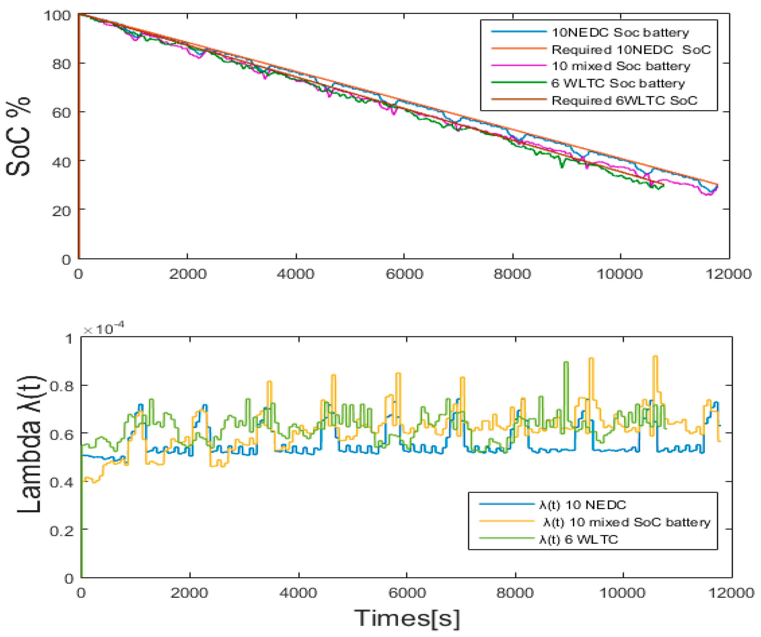
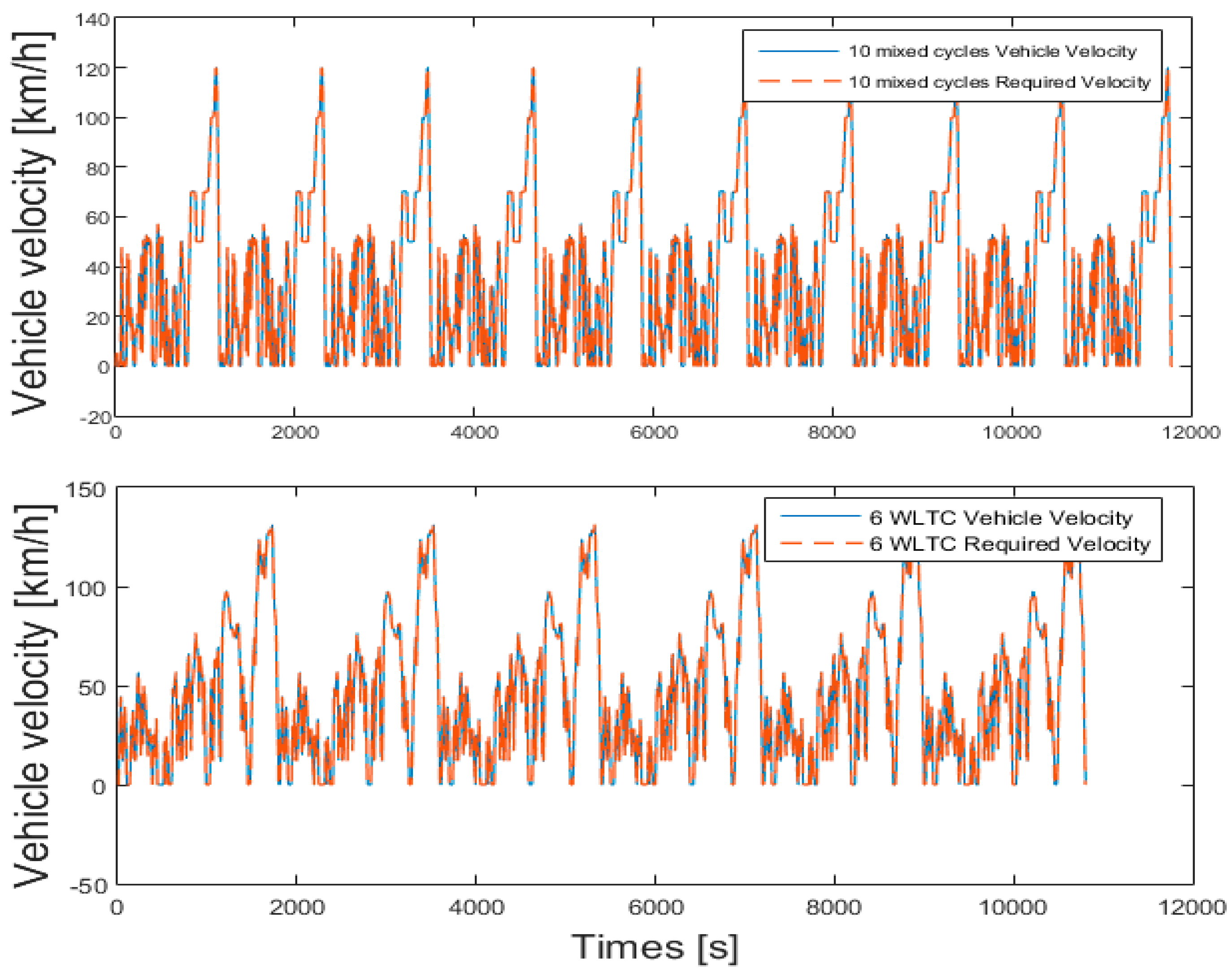
To test the robustness of the proposed λ-Control, two synthesized cycles are used. The first consists of ten consecutive mixed cycles that combine a hyzem urban cycle (Figure 4) with a EUC NEDC cycle (Figure 3). The second is a succession of six WLTC cycles. Figure 15 shows the state of charge SoC, the required SoC, and the multiplier variation of the proposed online L-Control algorithm for PHEV during ten MIXED cycles, six WLTC, and ten NEDC cycles. Figure 16 presents the vehicle velocity, the required vehicle velocity during ten MIXED cycles, and six WLTC of the proposed algorithm. Although the parameters have been conserved, curves indicate good SoC and vehicle speed tracking. It can be seen that the lambda variation depends on the driving cycle, but its variation is slightly perturbed. The amount of fuel consumed is around 2.33 L per 100 km for a battery balance of around −70.80% for ten mixed cycles (the best offline result is: 2.1 L for a battery balance of around −70.2%), which represents a gap of 0.10% in terms of fuel consumption and 0.6% in SoC per 100 km.

The amount of fuel consumed is around 2.87 L per 100 km for a battery balance of around −70.11% for 6 WLTC cycles (the best offline result of 2.7 L is for a battery balance of around −69.8%), allowing a small gap from optimal results (0.06% in terms of fuel consumption for a 0.31% in SoC per 100 km).

5. Conclusions

This article presents an efficient λ-control for an energy management strategy for PHEV derived from the PMP method. It has been extended from λ-control for HEV in charge-sustaining mode to be adequate for offline/online applications in the blended mode for parallel PHEV configuration. Offline-developed control uses a bisection method to search for the optimal control by assuming the existence of a lambda value that leads through every trip distance to a pre-defined SoC reference and is considered a benchmark for real-time techniques. For the online proposed control, an estimation of the initial multiplier is first proposed for a reference vehicle speed profile based on the energy power balance between vehicle powertrain components and the self-sufficiency assumption between the battery variation and its internal power. Then, this value is updated and adjusted to be adaptable in real-time using feedforward control striving to follow as much as possible a linear SoC reference and to ensure the total energy storage system depletion over the whole distance. In this sense, the co-state variation is dependent on how much the SoC variation is blended at the current time with respect to the adopted SoC reference.

Results approve for the proposed offline version an optimal fuel consumption rate, a good SoC variation performance, and how lambda affects the SoC variation. In real-time use, results also reveal a good velocity speed and SoC management. For the various test cycles, it’s proven how the quality of tracking SoC changes the lambda line form, which in turn affects the energy power-split control and thus the system performances. The effectiveness and the robustness of the proposed λ-control are then confirmed, while further fine-tuning may be needed later for the update and adjustment parameters. Even though the estimated initial multiplier value is different from the value found that leads to optimum, the results show an engine energy consumption savings close to the one obtained offline for an ultimate state of charge equal to 30%. In the present work, some issues have not been covered, such as the repartition of energy recovery during braking and deceleration or battery degradation due to intensive use. Only the effectiveness and robustness of the control are evaluated here, considering some assumptions to be improved. Introducing other aspects or considering multi-objective optimization control can be explored in coming studies. The obtained online results, close to the absolute optimum, present already good robustness behavior, which is promising for real-time use and the introduction of more criteria and constraints.

References

- Oumaima, M.; el Amraoui, L.; Trigui, R. Impact of Rule-based EMS parameters and charging strategies on Plug-in HEV efficiency. In Proceedings of the 2021 IEEE Vehicle Power and Propulsion Conference (VPPC), Gijon, Spain, 25–28 October 2021; IEEE: Piscataway, NJ, USA, 2021. [Google Scholar]
- Wirasingha, S.G.; Emadi, A. Classification and review of control strategies for plug-in hybrid electric vehicles. IEEE Trans. Veh. Technol. 2010, 60, 111–122. [Google Scholar] [CrossRef]
- Larsson, V.; Johannesson, L.; Egardt, B. Impact of trip length uncertainty on optimal discharging strategies for PHEVs. In Proceedings of the AAC’10—IFAC Symposium on Advances in Automotive Control, Munich, Germany, 12–14 July 2010. [Google Scholar]
- Vajedi, M.; Taghavipour, A.; Azad, N.L.; McPhee, J. A comparative analysis of route-based power management strategies for real-time application in plug-in hybrid electric vehicles. In Proceedings of the 2014 American Control Conferenc, Portland, OR, USA, 4–6 June 2014; IEEE: Piscataway, NJ, USA, 2014. [Google Scholar]
- Sciarretta, A.; Serrao, L.; Dewangan, P.; Tona, P.; Bergshoeff, E.; Bordons, C.; Charmpa, L.; Elbert, P.; Eriksson, L.; Hofman, T.; et al. A control benchmark on the energy management of a plug-in hybrid electric vehicle. Control. Eng. Pract. 2014, 29, 287–298. [Google Scholar] [CrossRef] [Green Version]
- Rousseau, A.; Pagerit, S.; Gao, D.W. Plug-in hybrid electric vehicle control strategy parameter optimization. J. Asian Electr. Veh. 2008, 6, 1125–1133. [Google Scholar] [CrossRef] [Green Version]
- Liu, L.; Zhang, B.; Liang, H. Global Optimal Control Strategy of PHEV Based on Dynamic Programming. In Proceedings of the 2019 6th International Conference on Information Science and Control Engineering (ICISCE), Shanghai, China, 20–22 December 2019; pp. 758–762. [Google Scholar] [CrossRef]
- Cui, L.; Jianhua, G.; Wei, Z.; Kangjie, L. Research on AECMS Energy Management Strategy of PHEV. In Proceedings of the 2019 IEEE 3rd Information Technology, Networking, Electronic and Automation Control Conference (ITNEC), Chengdu, China, 15–17 March 2019; pp. 500–504. [Google Scholar] [CrossRef]
- Lin, X.; Zhou, K.; Mo, L.; Li, H. Intelligent Energy Management Strategy Based on an Improved Reinforcement Learning Algorithm With Exploration Factor for a Plug-in PHEV. IEEE Trans. Intell. Transp. Syst. 2022, 23, 8725–8735. [Google Scholar] [CrossRef]
- Liu, C.; Murphey, Y.L. Optimal Power Management Based on Q-Learning and Neuro-Dynamic Programming for Plug-in Hybrid Electric Vehicles. IEEE Trans. Neural Netw. Learn. Syst. 2020, 31, 1942–1954. [Google Scholar] [CrossRef]
- Taghavipour, A. Predictive power management strategy for a PHEV based on different levels of trip information. IFAC Proc. Vol. 2012, 45, 326–333. [Google Scholar] [CrossRef]
- Joud, L. Stratégie Intelligente de Gestion du Système Energétique Global d’un Véhicule Hybride. Ph.D. Thesis, University of Franche-Comté, Besançon, France, 2018. [Google Scholar]
- Li, P. An Intelligent Logic Rule-Based Energy Management Strategy for Power-Split Plug-in Hybrid Electric Vehicle. In Proceedings of the 2018 37th Chinese Control Conference (CCC), Wuhan, China, 25–27 July 2018; IEEE: Piscataway, NJ, USA, 2018. [Google Scholar]
- Yu, H. Fuzzy logic energy management strategy based on genetic algorithm for plug-in hybrid electric vehicles. In Proceedings of the 2019 3rd Conference on Vehicle Control and Intelligence (CVCI), Hefei, China, 21–22 September 2019; IEEE: Piscataway, NJ, USA, 2019. [Google Scholar]
- Pu, Z.; Jiao, X.; Yang, C.; Fang, S. An adaptive stochastic model predictive control strategy for a plug-in hybrid electric bus during the vehicle-following scenario. IEEE Access 2020, 8, 13887–13897. [Google Scholar] [CrossRef]
- Martinez, C.M.; Hu, X.; Cao, D.; Velenis, E.; Gao, B.; Wellers, M. Energy management in plug-in hybrid electric vehicles: Recent progress and a connected vehicles perspective. IEEE Trans. Veh. Technol. 2016, 66, 4534–4549. [Google Scholar] [CrossRef]
- Sivertsson, M.; Eriksson, L. Design and evaluation of energy management using map-based ECMS for the PHEV benchmark. Oil Gas Sci. Technol. Rev. D’ifp Energ. Nouv. 2015, 70, 195–211. [Google Scholar] [CrossRef] [Green Version]
- Sivertsson, M. Adaptive control using map-based ECMS for a PHEV. IFAC Proc. 2012, 45, 357–362. [Google Scholar] [CrossRef] [Green Version]
- Guardiola, C.; Pla, B.; Onori, S.; Rizzoni, G. A new approach to optimally tune the control strategy for hybrid vehicles applications. IFAC Proc. Vol. 2012, 45, 255–261. [Google Scholar] [CrossRef]
- Schmid, R.; Buerger, J.; Bajcinca, N. Energy Management Strategy for Plug-in-Hybrid Electric Vehicles Based on Predictive PMP. IEEE Trans. Control. Syst. Technol. 2021, 29, 2548–2560. [Google Scholar] [CrossRef]
- Kermani, S. Gestion Energétique des Véhicules Hybrides: De la Simulation à la Commande Temps Réel; Université de Valenciennes et du Hainaut-Cambresis: Valenciennes, France, 2009. [Google Scholar]
- Hamidi Hedi, M. Contrôle Optimal de L’énergie Electrique Dans un Véhicule Hybride: Application à L’éco-Conduite. Ph.D. Thesis, National Engineering School of Carthage, Carthage, Tunis, 2020. [Google Scholar]
- Geitner, G.-H. The Bond Graph-an excellent modelling tool to study abstraction level and structure comparison. In Proceedings of the 2010 IEEE Vehicle Power and Propulsion Conference, Lille, France, 1–3 September 2010; IEEE: Piscataway, NJ, USA, 2010. [Google Scholar]
- Marquis-Favre, W. Mechatronic bond graph modelling of an automotive vehicle. Math. Comput. Model. Dyn. Syst. 2006, 12, 189–202. [Google Scholar] [CrossRef]
- Lhomme, W.; Trigui, R.; Delarue, P.; Jeanneret, B.; Bouscayrol, A.; Badin, F. Switched causal modeling of transmission with clutch in hybrid electric vehicles. IEEE Trans. Veh. Technol. 2008, 57, 2081–2088. [Google Scholar] [CrossRef]
- Letrouve, T. Structuration de la Commande de la Simulation au Prototype d’un Véhicule Hybride Double Parallèle au Travers de la Représentation Energétique Macroscopique. Ph.D. Thesis, Université Lille I, Lille, France, 2013. [Google Scholar]
- Castaings, A.; Lhomme, W.; Trigui, R.; Bouscayrol, A. Energy management of a multi-source vehicle by λ-control. Appl. Sci. 2020, 10, 6541. [Google Scholar] [CrossRef]
- Trigui, R.; Scordia, J.; Desbois-Renaudin, M.; Jeanneret, B.; Badin, F.; Plasse, C. Global Forward-Backward Approach for a Systematic Analysis and Implementation of Hybrid Vehicle Management Laws. Application to a Two Clutches Parallel Hybrid Power Train. In Proceedings of the EET-2004 European Ele-Drive Conference, Estoril, Portugal, 18–20 March 2004. [Google Scholar]
- Jeanneret, B.; Trigui, R. New Hybrid concept simulation tools, evaluation on the Toyota Prius car. In Proceedings of the 16th International Electric Vehicle Symposium, Beijing, China, 13–16 October 1999. [Google Scholar]
- Vinot, E. Model simulation, validation and case study of the 2004 THS of Toyota Prius. Int. J. Veh. Syst. Model. Test. 2008, 3, 139–167. [Google Scholar] [CrossRef]
- Katkar, V.A.; Goswami, P. Review on Energy Management Systems for Hybrid E Vehicles. In Proceedings of the 2020 International Conference on Power, Energy, Control and Transmission Systems (ICPECTS), Chennai, India, 10–11 December 2020; pp. 1–6. [Google Scholar] [CrossRef]
- Trigui, R. Approche Systémique Pour la Modélisation, la Gestion de L’énergie et L’aide au Dimensionnement des Véhicules Hybrides Thermiques-Electriques; Université des Sciences et Technologies de Lille: Lille, France, 2011. [Google Scholar]
- Yi, F.; Lu, D.; Wang, X.; Pan, C.; Tao, Y.; Zhou, J.; Zhao, C. Energy Management Strategy for Hybrid Energy Storage Electric Vehicles Based on Pontryagin’s Minimum Principle Considering Battery Degradation. Sustainability 2022, 14, 1214. [Google Scholar] [CrossRef]
- Zhou, J.; Feng, C.; Su, Q.; Jiang, S.; Fan, Z.; Ruan, J.; Sun, S.; Hu, L. The Multi-Objective Optimization of Powertrain Design and Energy Management Strategy for Fuel Cell–Battery Electric Vehicle. Sustainability 2022, 14, 6320. [Google Scholar] [CrossRef]
- Sandrini, G.; Chindamo, D.; Gadola, M. Regenerative Braking Logic That Maximizes Energy Recovery Ensuring the Vehicle Stability. Energies 2022, 15, 5846. [Google Scholar] [CrossRef]
- Kessel, J. Energy Management for Automotive Power Nets. Ph.D. Thesis, Technische Universiteit Eindhoven, Eindhoven, The Netherlands, 2006. [Google Scholar]
- Koot, M.; Kessels, J.; De Jager, B. Fuel reduction of parallel hybrid electric vehicles. In Proceedings of the 2005 IEEE Vehicle Power and Propulsion Conference, Chicago, IL, USA, 7 September 2005; IEEE: Piscataway, NJ, USA, 2005. [Google Scholar]
- Kermani, S.; Delprat, S. A comparison of two global optimization algorithms for hybrid vehicle energy management. In Proceedings of the IFAC IEEE 2007 International Conference on Advances in Vehicle Control and Safety AVCS’07, Buenos Aires, Argentina, 8–10 February 2007. [Google Scholar]
- Delprat, S. Evaluation de Stratégies de Commande pour Véhicules Hybride Paralleles; Université de Valenciennes et du Hainaut-Cambresis: Valenciennes, France, 2002. [Google Scholar]
- Stroe, N. Contributions to Model-Based Predictive Energy Management in Hybrid Electric Vehicles; Université d’Orléans: d’Orléans, France, 2017. [Google Scholar]
Figure 1.
Variation of the state of charge of the battery during the three modes of operation for a PHEV.
Figure 2.
European standard cycle NEDC.
Figure 3.
European Standard cycle WLTC (CLASSE3/BV).
Figure 4.
Urban Hyzem cycle, Road Hyzem cycle, and Highway Hyzem cycle.
Figure 5.
The global EMS-Parallel-PHEV model presenting four main sub-blocks.
Figure 6.
Electric motor cartography presenting power loss within EM torque and speed limits.
Figure 7.
ICE cartography presenting fuel flow within engine torque and speed limits.
Figure 8.
Diagram of an offline L-Control calculation using the Bisection method.
Figure 9.
Input/output power energy for a parallel PHEV Topology.
Figure 10.
Diagram of an online L-Control calculation.
Figure 11.
State of the charge variation according to L-Control parameters iteration using the Bisection method in the offline calculation.
Figure 12.
Validation of the proposed offline L-Control algorithm for PHEV during 10 NEDC cycles.
Figure 13.
Validation of the proposed online L-Control algorithm for PHEV during 10 NEDC cycles.
Figure 14.
ICE operating point variation of the proposed L-Control algorithm and Rl-based strategy.
Figure 15.
SoC and lambda variation of the proposed online L-Control algorithm for PHEV during 10 MIXED cycles, 6 WLTC, and 10 NEDC cycles.
Figure 16.
Vehicle velocity and required velocity variation of the proposed online L-Control algorithm for PHEV during 10 MIXED cycles, 6 WLTC, and 10 NEDC cycles.