Prediction of In-Cylinder Pressure of Diesel Engine Based on Extreme Gradient Boosting and Sparrow Search Algorithm

Abstract

In-cylinder pressure is one of the most important references in the process of diesel engine performance optimization. In order to acquire effective in-cylinder pressure value, many physical tests are required. The cost of physical testing is high; various uncertain factors will bring errors to test results, and the time of an engine test is so long that the test results cannot meet the real-time requirement. Therefore, it is necessary to develop technology with high accuracy and a fast response to predict the in-cylinder pressure of diesel engines. In this paper, the in-cylinder pressure values of a high-speed diesel engine under different conditions are used to train the extreme gradient boosting model, and the sparrow search algorithm—which belongs to the swarm intelligence optimization algorithm—is introduced to optimize the hyper parameters of the model. The research results show that the extreme gradient boosting model combined with the sparrow search algorithm can predict the in-cylinder pressure under each verification condition with high accuracy, and the proportion of the samples which prediction error is less than 10% in the validation set is 94%. In the process of model optimization, it is found that compared with the grid search method, the sparrow search algorithm has stronger hyper parameter optimization ability, which reduces the mean square error of the prediction model by 27.99%.

1. Introduction

As a stable and efficient power source, diesel engine plays an important role in industry, agriculture and transportation. Since the advent of the world’s first diesel engine, researchers have been committed to improving the performance of the diesel engine to meet more severe application conditions. The combustion condition in the cylinder is directly related to the power output and emission level of the diesel engine. In order to analyze and optimize the combustion process of the diesel engine, the most commonly used method is to measure the in-cylinder pressure. By analyzing the heat release rate according to the in-cylinder pressure, the variation characteristics of many parameters in the combustion process can be acquired. In the development and calibration stage of diesel engines, the cylinder pressure is a very valuable reference indicator, which is of great significance to improve power and economy, reduce noise and emissions and reduce failure probability for engines [1]. Frank Willems proposed that real-time closed-loop control of in-cylinder pressure is one of the effective methods to achieve efficient and clean combustion of diesel engines in the future [2], and the control of combustion phase and heat release is the key to ensure stable and efficient operation of engines. Marcus Klein et al. proposed four real-time estimation methods of a compression ratio based on an in-cylinder pressure track, and used the estimation method to evaluate the simulation cycle and test cycle, which improved the stability of the variable compression ratio engine [3]. A.J. Torregosa et al. proposed and verified a method for diagnosing noise sources by extracting appropriate components from in-cylinder pressure, which can accurately predict the noise level of diesel engines and identify noise-related combustion characteristic parameters [4]. Yuan et al. studied the relationship between the diesel engine combustion noise and the double-peak characteristics of the cylinder pressure rise rate, and the results showed that the second peak is the characteristic quantity of the combustion noise, and the combustion noise is a function of the diesel engine load [5]. He et al. calculated CA50 (Phase of 50% heat release) according to the in-cylinder pressure, and analyzed the relationship between CA50 and NOx emission. The results showed that NOx emission and CA50 had a certain logarithmic function relationship [6]. Yang et al. calculated various combustion characteristic parameters according to the cylinder pressure, and ECU adjusted the fuel injection parameters according to the combustion characteristic parameters, which significantly improved the combustion stability in the cylinder and the non-uniformity of each cylinder [7]. The above research proves the importance of cylinder pressure in the process of diesel engine performance optimization. However, the acquisition of cylinder pressure data currently relies on many physical tests, the test cost is high, and there are many uncertain factors in the test process, which is prone to measurement errors. Moreover, the test time is long, and the measurement results cannot meet the real-time requirements. Therefore, it is very important to develop a high-accuracy and fast-responding technology to predict the in-cylinder pressure of diesel engines.

With the rapid development of data science and artificial intelligence, machine learning, as the core of artificial intelligence, has been widely used in finance, Internet, medicine, and other fields [8,9,10]. Machine learning refers to computers continuously refining and summarizing knowledge from data by simulating human learning behavior, thereby adjusting their structure to achieve or even surpass human intelligence. Compared with experimental measurement and physical calculation models, machine learning has advantages such as fast response, high accuracy, and strong generalization ability [11,12]. In recent years, because of its powerful induction and reasoning capabilities, machine learning has been gradually applied to pattern recognition and performance optimization of engines [13,14,15,16,17]. Jihad A. Badra et al. developed a Machine Learning Grid Gradient Ascent (ML-GGA) approach to optimize the performance of internal combustion engines and demonstrated the potential of ML-GGA to significantly reduce the time needed for optimization problems, without a loss of accuracy compared with traditional approaches [18]. Kowalski J et al. proposed a fully automatic engine fault detection system based on machine learning. The experimental results show that the method has high classification accuracy and a low response time [19]. Wong P K et al. proposed a new model and optimization framework for a biodiesel engine based on extreme learning machine (ELM), and used a cuckoo search (CS) to determine the optimal biodiesel ratio. The results show that the model can accurately predict engine performance [20]. Noor C. et al. conducted artificial neural network modeling for marine diesel engines to predict performance parameters such as output torque, power, specific fuel consumption, and exhaust temperature. The model prediction results were in good agreement with the experimental results, and the coefficient of determination R² reached 0.99 [21]. Yusaf T.F. et al. used an artificial neural network to predict the performance of a CNG–diesel dual-fuel engine, and all performance parameters achieved good prediction results [22].

Machine learning has been widely proven to have strong abstraction capabilities and can effectively solve high-dimensional and nonlinear problems, and many research findings have been obtained in the performance prediction of diesel engines. However, there is seldom research on the prediction of diesel engine cylinder pressure, and existing studies prefer to choose an artificial neural network as the prediction model when predicting the performance of diesel engine. Although the prediction ability of artificial neural network is strong, there are some defects such as complex model structure, poor interpretability, high training cost, and high risk of overfitting [23,24]. Therefore, in order to realize the accurate prediction of the in-cylinder pressure of the diesel engine, this paper acquired the in-cylinder pressure data of the diesel engine under different steady-state conditions through bench tests. The extreme gradient boosting model in ensemble learning is trained with the in-cylinder pressure data. Considering that there are many hyper parameters of the prediction model and the adjustment process is very complex, in order to simplify the process of hyper parameter adjustment and improve the prediction accuracy of the model, the sparrow search algorithm in a swarm intelligence optimization algorithm was used to optimize the hyper parameters of the model.

2. Materials and Methods

2.1. Experiment and Data Acquisition

The test object of this study is a supercharged and intercooled high-speed diesel engine. The detailed engine specifications are summarized in

Table 1. Test engines specifications.

Description	Specification
Rated speed/power	2200 rpm/142 kW
NO. Cylinder	4
NO. Stroke	4
Displacement	5.1 L
Bore	110 mm
Stroke	135 mm
Compression ratio	19.05
Cylinder arrangement	V-type

.

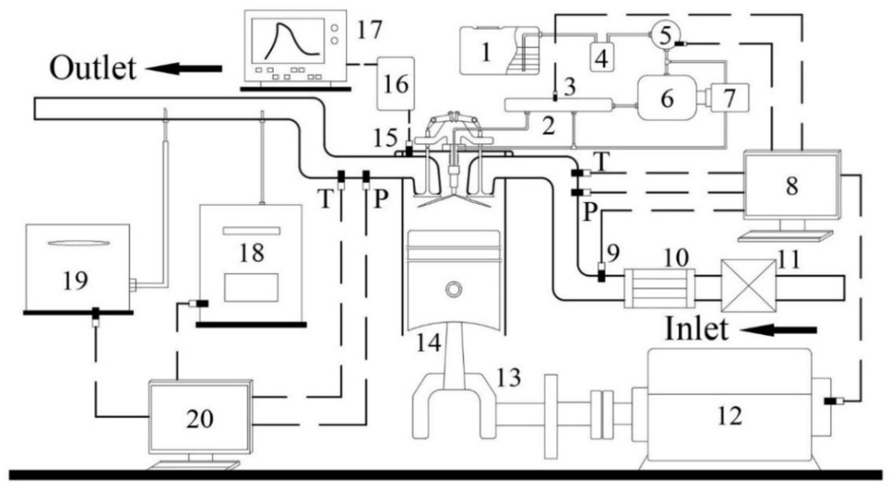
The schematic diagram of the experimental set-up is presented in Figure 1.

In the steady-state tests of the diesel engine, it was necessary to control the variables in the tests. The intake air temperature was maintained at (25 ± 2) °C by the air conditioner, the air humidity was maintained at ~50%, and the air intake pressure was (101 ± 1) kPa. The exhaust pressure of the engine was maintained at (10 ± 0.5) kPa. The cooling mode of the engine was water cooling, and the cooling water temperature was maintained at ~(85 ± 5) °C. The fuel used in the tested engine was China VI 0# diesel. During the tests, the Kistler 6125c cylinder pressure sensor was used for cylinder pressure measurement. The installation position of the cylinder pressure sensor was located in the cylinder head of the first cylinder and connected with the charge amplifier. The pressure signal was amplified by the charge amplifier and transmitted to the combustion analyzer. At the same time, the Kistler angle scale was used to identify the TDC (Top Dead Center) and CA (crank angle) signal. The measuring range of the Kistler 6125c cylinder pressure sensor is 0~300 bar and the deviation is ±1%. In this study, the in-cylinder pressure was collected every 0.5° crank angle, variation of crank angle from −360 to 360°, and a total of 1441 samples were collected in a single engine cycle. The in-cylinder pressure value with a crank angle was recorded from 100 engine cycles under each operating condition. The main instrumentation specifications used on the test bench are summarized in

Table 2. Test bench instrumentations.

Instrumentation	Type	Deviation
Dynamometer	AVL INDY S22-4	±0.3%
Air flowmeter	ABB-0(40) …1200 kg	±0.1%
Cylinder pressure sensor	Kistler 6125C	±1%
Combustion analyzer	Kistler DEWE	-
Fuel consumption meter	AVL 735S	±0.5%

.

The selected operating conditions are shown in

Table 3. Test conditions of the engine.

Speed	Load Rate
2200 rpm	10–100% (interval 10%)
1600 rpm
1200 rpm

. The in-cylinder pressure values under 30 operating conditions were collected.

2.2. Theory of Algorithms

2.2.1. Extreme Gradient Boosting

XGB (Extreme Gradient Boosting) trains multiple decision trees in series. Each decision tree learns from the previous decision tree and generates the final prediction result by synthesizing the decision values of all weak learners. XGB expands the loss function using a second-order Taylor series and introduces the regular term to avoid overfitting of the model [25]. Figure 2 is the schematic diagram of XGB model.

Each round of training in boosting will add a new function to the model. The objective function is shown as Equation (1).

$$Ob{j}^{\left(t\right)}={\displaystyle \sum }_{i=1}^{n}l(y_i,{{\widehat{y}}_i}^{(t-1)}+f_t\left(x_i\right))+\Omega \left(f_t\right)+constant$$

(1)

where $t$ is the number of training rounds; $f_t\left(x_i\right)$ represents the t-th regression tree; $\Omega \left(f_t\right)$ is the penalty term and $constant$ is the constant term.

Expand the objective function with Taylor series, and the result is shown in Equation (2):

$$Ob{j}^{\left(t\right)}\widetilde{-}{\displaystyle \sum }_{i=1}^n\left[l\left(y_i,{{\widehat{y}}_i}^{(t-1)}\right)+g_i{f}_t\left(x_i\right)+\frac{1}{2}{h}_i{f_t}^2\left(x_i\right)\right]+\Omega \left(f_t\right)+constant$$

(2)

where $g_i$ is the first derivative, $h_i$ is the second derivative.

The penalty term is defined as Equation (3):

$$\Omega \left(f_t\right)=\gamma T+\frac{1}{2}\lambda {\displaystyle \sum }_{j=1}^T{w_j}^2$$

(3)

where $T$ is the number of leaf nodes and $w_j$ represents the weight of the j-th leaf node.

The objective function can be reduced to Equation (4):

$$\begin{gathered} Ob{j}^{\left(t\right)}={\displaystyle \sum }_{j=1}^T\left[\left({{\displaystyle \sum }}_{i\in I_j}{g}_i\right)w_j+\frac{1}{2}\left({{\displaystyle \sum }}_{i\in I_j}{h}_i+\lambda \right){w_j}^2\right]+\gamma T \\ ={\displaystyle \sum }_{j=1}^T\left[G_j{w}_j+\frac{1}{2}\left(H_j+\lambda \right){w_j}^2\right]+\gamma T \end{gathered}$$

(4)

2.2.2. Sparrow Search Algorithm

SSA (Sparrow Search Algorithm) is a new swarm intelligence optimization algorithm. Its design inspiration comes from the group foraging behavior of the sparrow population in nature. Individuals in the sparrow population adapt to the environment by constantly adjusting their distribution position, so as to obtain better food resources and avoid the attack of predators [26]. The sparrow search algorithm has been shown to outperform many traditional population intelligence optimization algorithms in terms of its ability to find the best and avoid being trapped in local extremes [27,28]. The mathematical model of SSA is as follows:

In the simulated population, assuming that the virtual sparrow is foraging, the sparrow population composed of N sparrows can be represented by matrix (5):

$$X=\left[\begin{array}{cccc}{x}_{1,1}& x_{1,2}& \cdots & x_{1,d}\\ x_{2,1}& x_{2,2}& \cdots & x_{2,d}\\ ⋮& ⋮& ⋮& ⋮\\ x_{n,1}& x_{n,2}& \cdots & x_{n,d}\end{array}\right]$$

(5)

where n signifies the number of all sparrows in the population and d describes the dimension of the decision variables.

The fitness values of all sparrows can be expressed by Equation (6):

$$F_X=\left[\begin{array}{c}f\left[\begin{array}{cccc}{x}_{1,1}& x_{1,2}& \cdots & x_{1,d}\end{array}\right]\\ f\left[\begin{array}{cccc}{x}_{2,1}& x_{2,2}& \cdots & x_{2,d}\end{array}\right]\\ ⋮\\ ⋮\\ f\left[\begin{array}{cccc}{x}_{n,1}& x_{n,2}& \cdots & x_{n,d}\end{array}\right]\end{array}\right]$$

(6)

Sparrow populations are divided into producers and scroungers. Producers have higher energy reserves and are responsible for searching for areas with more food, providing foraging areas and directions for scroungers. When individual sparrows detect predators, they will sound an alarm signal. If the alarm value is higher than the safety value, the producers will take the scroungers to a safe area for foraging. In the iterative process of the algorithm, the update rule of the producer’s position is shown in Equation (7):

$$X_{i,j}^{t+1}=\{\begin{array}{c}{X}_{i,j}^t·\exp \left(-\frac{i}{\alpha ·M}\right) if R_2<ST\hfill \\ X_{i,j}^t+Q·L if R_2\ge ST\hfill \end{array}$$

(7)

where $t$ is the current number of iterations, $X_{ij}$ is the location information of the sparrows, $\alpha$ is a random number with a value range of [0, 1], $M$ is the maximum number of iterations, $Q$ is a random number which obeys to normal distribution, and $L$ is a $1\times d$ matrix, in which the elements are all 1. $R_2\in \left[0, 1\right], ST\in \left[0.5, 1\right]$, respectively represent safety value and alarm value; when $R_2<ST$, there is no predator invasion, and the producers can carry out a wide range of search operations. When $R_2\ge ST$, it means that the individuals in the population have detected the predators, and all sparrows need to fly to a safe area immediately.

Scroungers will keep an eye on the producers. Once the producers find a better foraging area, the scroungers will immediately compete with them. If the scroungers win, they will seize the resources from producers instantly. The rule for updating the scrounger’s location is as follows:

$$X_{i,j}^{t+1}=\{\begin{array}{c}Q·\exp \left(\frac{X_{worst}-X_{i,j}^t}{i^2}\right) if i>\frac{n}{2}\hfill \\ X_p^{t+1}+\left|X_{i,j}^t-X_p^{t+1}\right|·A^{+}·L otherwise\hfill \end{array}$$

(8)

where $X_p$ is the best position occupied by the current producers, $X_{worst}$ is the global worst position, and r. $A$ describes a $1\times d$ vector such that the elements are randomly assigned 1 or −1, $A^{+}=A^T{\left(A{A}^T\right)}^{-1}$, and n is the total number of sparrows in the populations. When $i>n/2$, it means that the i-th scroungers with low fitness do not get any food and need to fly to other areas for foraging.

The initial positions of the sparrows which are aware of the danger are as follows:

$$X_{i,j}^{t+1}=\{\begin{array}{c}{X}_{best}^t+\beta ·\left|X_{i,j}^t-X_{best}^t\right| if f_i>f_g\hfill \\ X_{i,j}^t+K·\left(\frac{X_{i,j}^t-X_{worst}^t}{f_i-f_w+\epsilon }\right) if f_i=f_g\hfill \end{array}$$

(9)

where, $\beta$ signifies a normal distributed random value with a mean value of 0 and a variance of 1. $\epsilon$ is the smallest constant for avoiding from zero-division-error. $K\in \left[-1, 1\right]$, is also a random number. $f_i$ is the fitness of the current individuals. $f_g$ and $f_w$ represent the current global best and worst fitness, respectively. When $f_i>f_g$, the sparrow is in a marginal position and vulnerable to predators. $f_i=f_g$ indicates that the sparrows in the population are aware of the danger and need to be close to other sparrows to avoid being caught by predators.

Figure 3 represents the iterative flow chart of SSA.

2.3. Model Establishment

Python language was used in the process of model building, the compilation environment is Pycharm, and the python libraries used mainly include scikit learn, pandas, numpy, Matplotlib, etc.

2.3.1. Input and Output Selection

Extreme gradient boosting belongs to supervised learning. During the training process of the model, input features and the output label of the model need to be determined. In order to realize the prediction of in-cylinder pressure under specific operating conditions of diesel engine, the in-cylinder pressure was selected as the output label for the models, and the excess air coefficient, speed, torque, power, fuel consumption and crank angle that could represent the characteristics of the operating conditions were chosen as the input features.

2.3.2. Split and Preprocessing of Datasets

Through the steady-state operating condition tests, the data under 30 operating conditions were acquired. Each condition contained 1441 samples of in-cylinder pressure. In this paper, the in-cylinder pressure values from 6 conditions were selected as the validation set to prove the predictive performance of the model. The validation operating conditions are represented in

Table 4. Engine conditions for validation set.

Validation Condition	Speed	Load	MEP 1
1	2200 rpm	100%	1.5 MPa
2		50%	0.9 MPa
3	1600 rpm	100%	1.8 MPa
4		50%	1.1 MPa
5	1200 rpm	100%	1.7 MPa
6		50%	1.0 MPa

¹ Mean Effective Pressure.

. In order to facilitate the description of these operating conditions in the later sections, they are numbered 1 to 6, respectively. A total of 34,584 samples from the remaining 24 operating conditions were randomly divided by the ratio of 8:2, of which 80% of the samples were used as the training set to train the model, and 20% of the samples were used as the test set.

In order to eliminate the dimensional differences between different features and reduce training cost of the model, it is necessary to process the original data. The preprocessing method selected in this study is normalization, which can render each feature dimensionless and scale the values in the range of [0, 1]. The normalization method is as in Equation (10):

$$\widehat{x}=\frac{x-x_{min}}{x_{max}-x_{min}}$$

(10)

where $x$ is the original data and $x_{min}$ is the minimum value of the feature; $x_{max}$ is the maximum value of the feature; $\widehat{x}$ represents the data after normalization.

The data description after preprocessing is shown in

Table 5. Data description after preprocessing.

Features	Count	Mean	Std	Min	25%	50%	75%	Max
φ 1	34,584	0.262	0.250	0	0.053	0.225	0.374	1
Speed	34,584	0.467	0.411	0	0.000	0.400	1.000	1
Torque	34,584	0.450	0.315	0	0.188	0.394	0.728	1
Power	34,584	0.409	0.287	0	0.164	0.371	0.608	1
FS 2	34,584	0.397	0.270	0	0.177	0.366	0.559	1
CA 3	34,584	0.500	0.289	0	0.250	0.500	0.750	1

¹ Excess air coefficient; ² fuel consumption; ³ crank angle.

.

2.3.3. Evaluation Criteria of the Model

In statistics, there are various statistical metrics used to evaluate the prediction performance of the model. This paper used four common metrics. These metrics are Mean Square Error (MSE), Root Mean Squares Error (RMSE), Mean Absolute Error (MAE), and Coefficient of Determination (R²). The equations and performance criteria of these metrics are shown in

Table 6. Description of evaluation metrics ¹.

Metric	Equation	Performance Criteria
MSE	$\frac{1}{n}{\displaystyle \sum _{i=1}^n}{\left({\widehat{y}}_i-y_i\right)}^2$	The smaller the MSE value, the higher the prediction accuracy of the model. The value range of MSE is [0, +∞].
RMSE	$\sqrt[2]{\frac{1}{n}{\displaystyle \sum _{i=1}^n}{\left({\widehat{y}}_i-y_i\right)}^2}$	RMSE is the arithmetic square root of MSE. The value range of RMSE is [0, +∞].
MAE	$\frac{1}{n}{\displaystyle \sum _{i=1}^n}\left|{\widehat{y}}_i-y_i\right|$	When the predicted value is completely consistent with the actual value, MAE is equal to 0. The greater the error, the greater the MAE, and the value range of MAE is [0, +∞].
R2	$\frac{{\sum }_{i=1}^n{\left({\widehat{y}}_i-\overline{y}\right)}^2}{{\sum }_{i=1}^n{\left(y_i-\overline{y}\right)}^2}$	The value range of R2 is [0, 1]. The closer it is to 1, the stronger the model’s ability to explain the predicted object. The closer it is to 0, the worse the fit of the model.

¹${\widehat{y}}_i$ is the predicted value, $y_i$ is the true value and $\overline{y}$ is the average of the true values.

.

3. Results and Discussion

3.1. Predictive Performance of the Initialized Model

The selection of hyper parameters has a significant influence on the predictive performance of machine learning models. However, there is currently no relevant theoretical support for hyper parameter selection, and the adjustment process of hyper parameters is usually extremely cumbersome. The main hyper parameters that need to be adjusted for the XGB model and their meanings are shown in

Table 7. Hyper parameters of XGB and their meanings.

Parameter	Meaning
max_depth	Depth of decision tree
n_estimators	Number of weak learners
eta	Learning rate
min_child_weight	Sum of minimum sample weights required by leaf nodes
gamma	The drop value of the minimum loss function required for node splitting

.

First, the predictive performance of the initialized XGB was analyzed. The five hyper parameters of the model, max_depth, n_estimators, eta, min_child_weight, and gamma, were set to 2, 100, 0.1, 3, and 0.1, respectively.

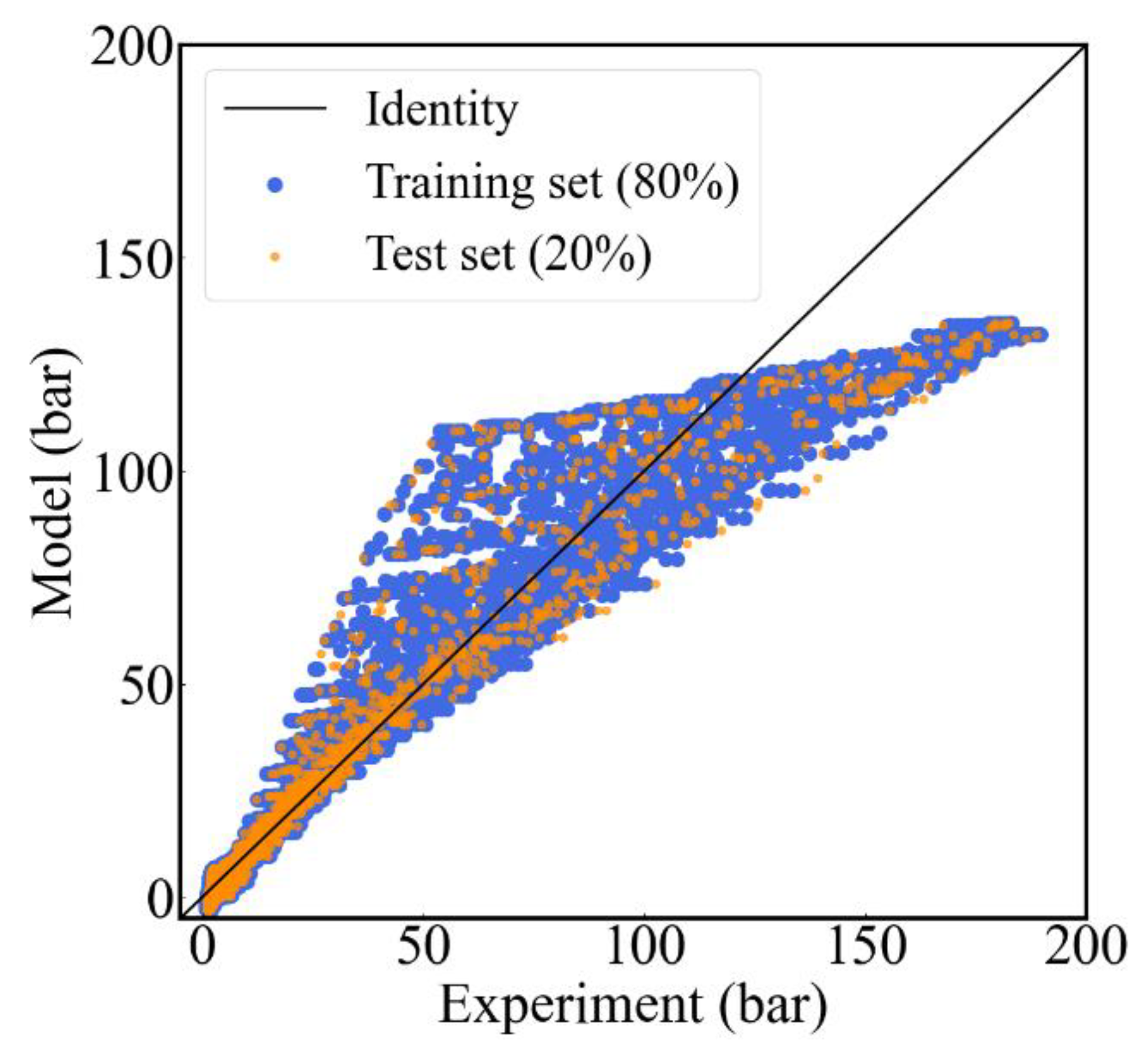
Figure 4 shows the results of the regression analysis of the initialized model, in which the blue scatter points represent the results of prediction for the training set, the orange scatter points represent the results of prediction for the test set, and the black straight line represents the 45° line where the predicted values are equal to the test values. The number of samples in the training set is 27,667 and the number of samples in the test set is 6917 according to the data set division ratio described in Section 2.3.2. It can be seen in Figure 4 that the prediction performance of the initialized model is poor, and the prediction results for samples with larger values are extremely inaccurate.

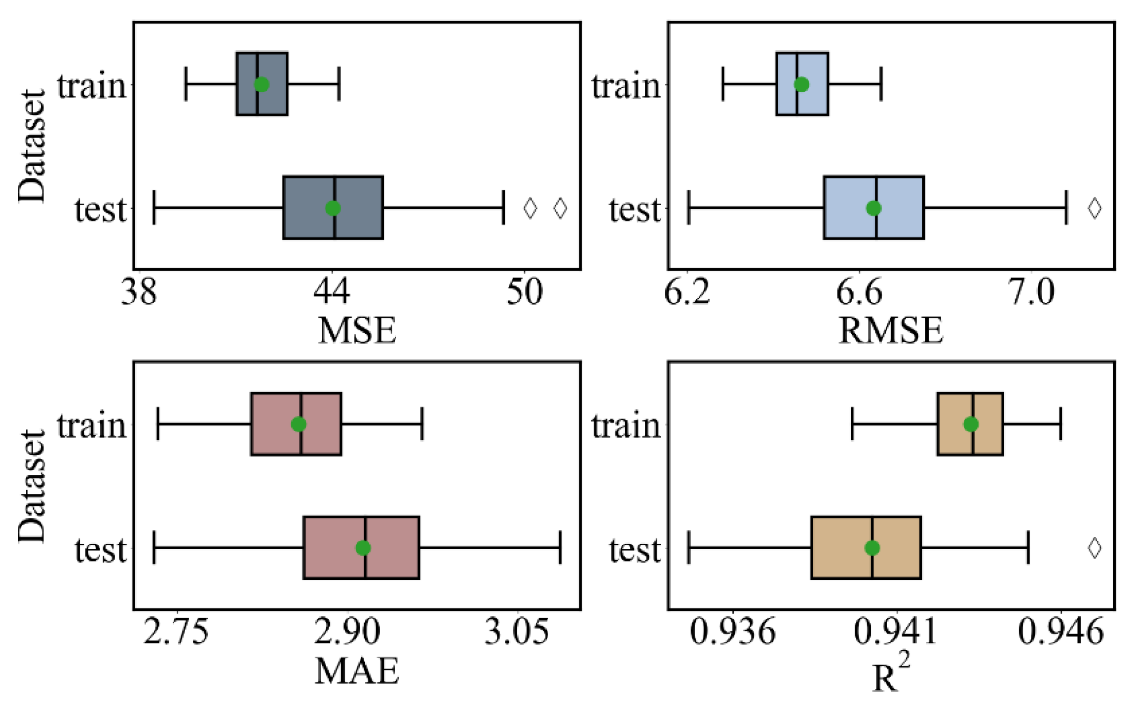
In order to comprehensively evaluate the performance of the initialized model, the data set was randomly divided in the ratio of 8:2, and a total of 100 training and testing processes were performed on the model, and then the evaluation results of each metric were calculated and recorded; the results are shown in Figure 5. The mean values of MSE, RMSE, MAE, and R² of the initialized model are 44.02, 41.81; 6.63, 6.47; 2.91, 2.86; 0.940, 0.943 (test set, training set), respectively.

3.2. Predictive Performance of the Optimized Model

The predictive performance of the initialized model was poor and insufficient for the purpose of in-cylinder pressure prediction, so the hyper parameters of the model needed to be optimized. The upper and lower bounds of the hyper parameters needed to be set before the optimization of the prediction model using the SSA. The upper and lower bounds of the five hyper parameters were empirically set to (10, 1000, 0.3, 10, 0.3) and (1, 100, 0.01, 1, 0.01), respectively. The dimension of the hyper parameters which need to be optimized was five, and the number of sparrow populations was set to 100. The fitness value was the sum of the MSE of the training set and test set; the fitness function is shown in Equation (11):

$$fitness=\left(MS{E}_{training}+MS{E}_{test}\right)$$

(11)

The optimization trajectory of SSA is shown in Figure 6. According to the optimization trajectory, it can be seen that the value of the optimal fitness of the population continued to decrease as the number of iterations increased, and the calculation converged when the number of iterations reached 10, which implies that the optimal value was found. The value of the minimal MSE was 0.05688, and the corresponding values of the five hyper parameters of the model were 8, 1000, 0.0688, 4.8015, and 0.01, respectively.

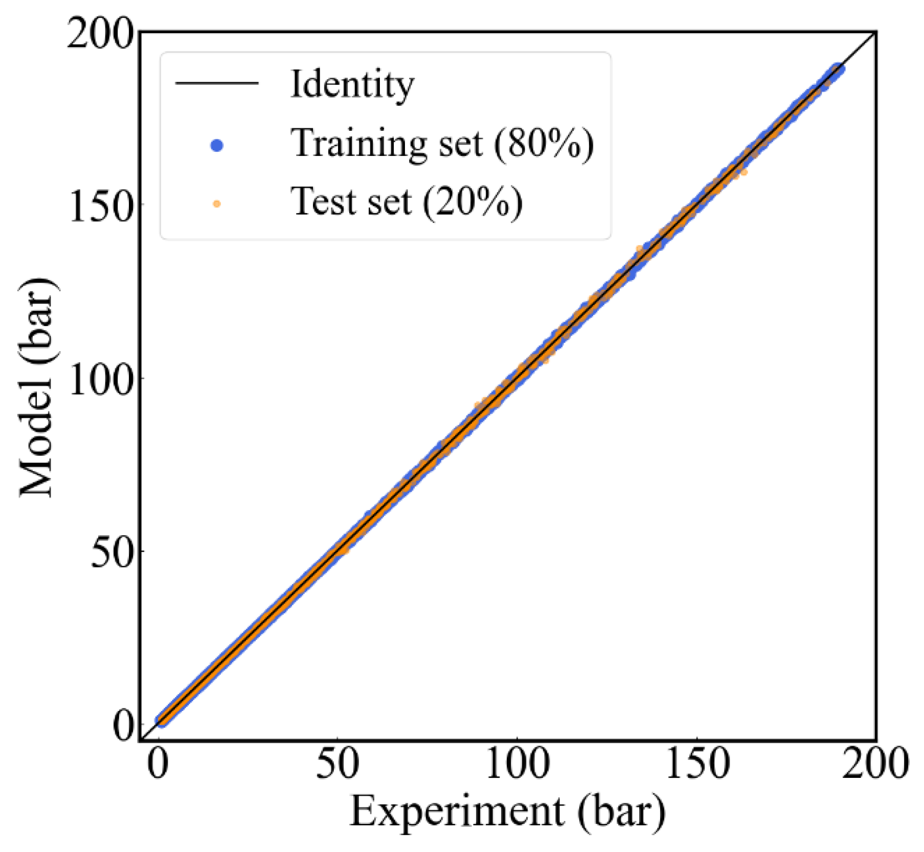
Figure 7 shows the results of the regression analysis of SSA-XGB. Both the training set and test set in the figure overlap with the diagonal line and achieve a good fit, indicating that the predictive performance of the model was significantly improved after the optimization of the hyper parameters.

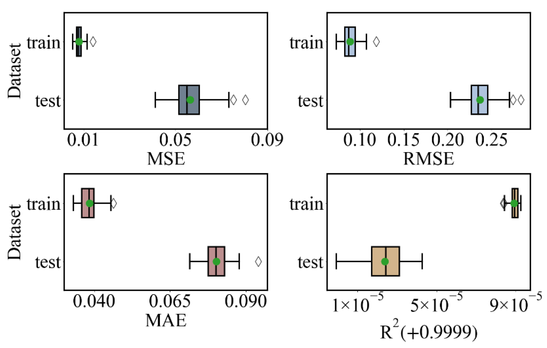
Figure 8 represents the evaluation results of the optimized model. Comparison with the evaluation results of the initialized model reveals that MSE, RMSE, and MAE all decreased significantly and the values were more stable, while the coefficient of determination R² reached more than 0.9999, and the mean values of each evaluation metric were 0.05635, 0.00797; 0.23689, 0.08891 0.08022, 0.03843; 0.99992, 0.99999 (test set, training set), respectively. The results fully demonstrate the predictive ability of the optimized XGB model.

Grid search is one of the most basic hyper parameter optimization algorithms. The basic principle is to adjust the parameters sequentially in steps within the specified parameters range, and use the adjusted parameters to train the prediction model until the optimal hyper parameters are found. Compared to swarm intelligence optimization algorithms, a traditional grid search method takes more computation time and may not always find the extremum of the objective function. Setting the step size of each hyper parameter of the model as (1,10,0.001,0.1,0.001), and then using the grid search to find the optimization of the hyper parameters, the minimum MSE of the model was 0.08077.

Table 8. Hyper parameters and MSE of the model.

	Max_Depth	n_Estimators	eta	Min_Child_Weight	Gamma	MSE (Train and Test)
Initial	2	100	0.1	3	0.1	90.370
Grid search	8	960	0.017	4.1	0.012	0.07899
SSA	8	1000	0.0688	4.8015	0.01	0.05688

presents the hyper parameters and MSE of initialized XGB, grid search-XGB and SSA-XGB; the MSE of the SSA-XGB model was reduced by 27.99% compared to use grid search method.

3.3. Prediction Results of the Validation Set

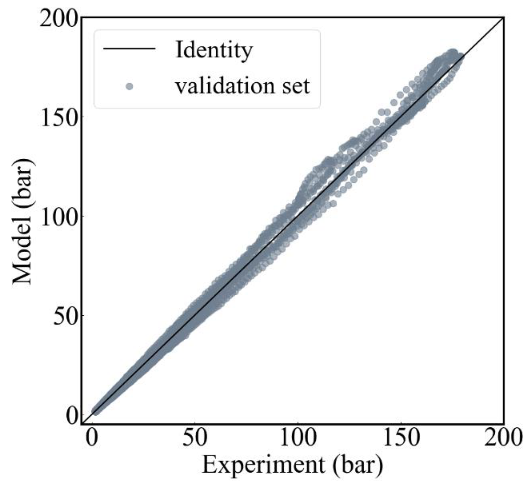
The validation set contains in-cylinder pressure data from six different operating conditions, of which there are 8646 samples. Using the optimized model to predict the validation set, the regression analysis is shown in Figure 9. As can be seen in Figure 9, most of the samples lie around the diagonal line, and only a few validation samples with larger values deviate, which means that the model obtained very accurate prediction results on the validation set.

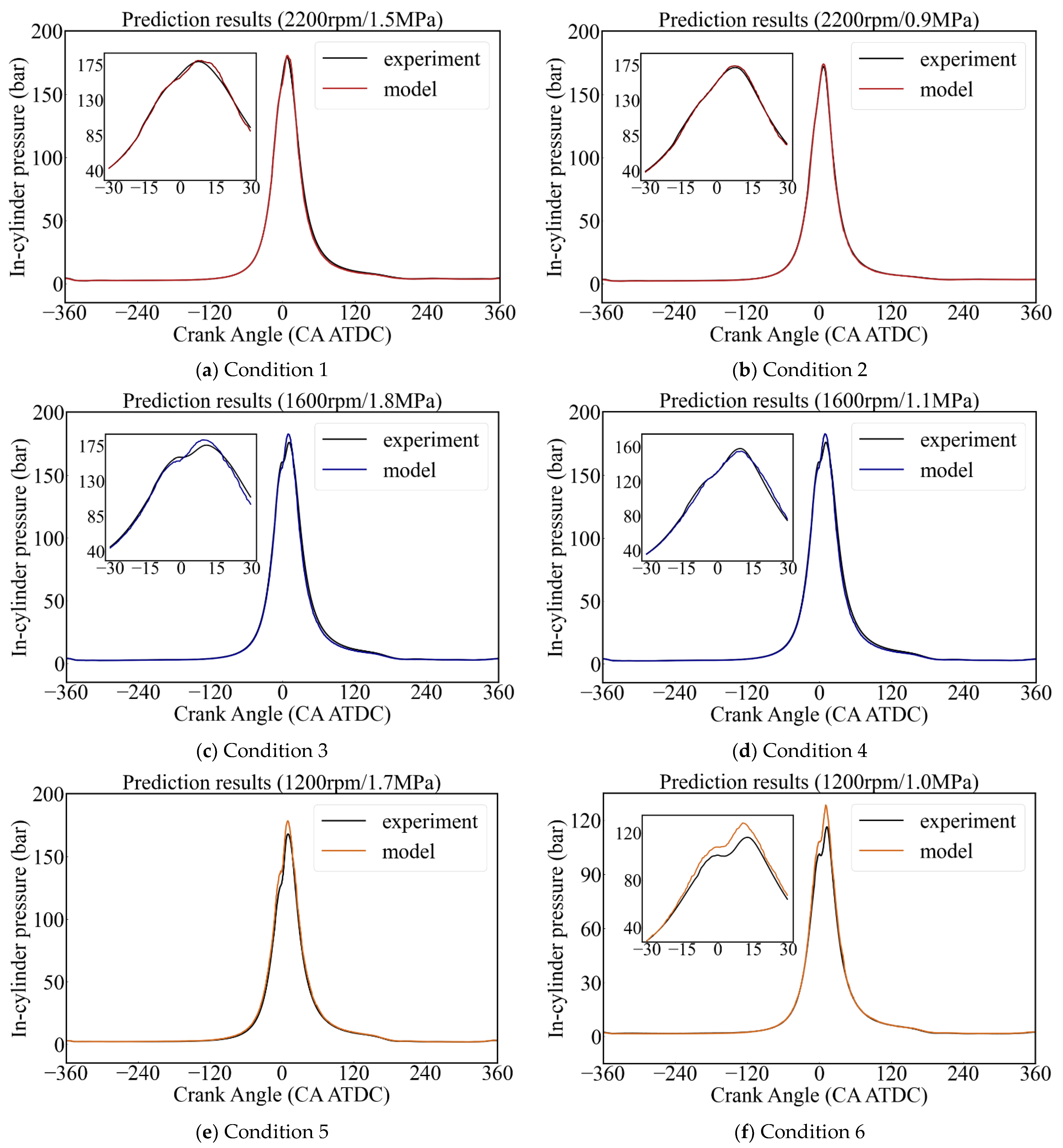
In order to represent the prediction results of the validation set more intuitively, the predicted values of each validation operating condition were fit to the actual values; the results are shown in Figure 10. The horizontal axis is the crank angle and the vertical axis is the in-cylinder pressure value. The black curve represents the actual value acquired in the tests, and the rest of the curves in different colors are the predicted values of the prediction model. As can be seen in Figure 10, the predicted values from operating condition 1, 2, and 4 are in good agreement with the actual values, and the predicted in-cylinder pressure values at the rest of the operating conditions only deviate from the actual values in the peak region.

3.4. Error Analysis

Figure 11 shows the results of the error analysis for the validation conditions. The horizontal axis of the figure is the crank angle, the vertical axis is the error value, the black horizontal line indicates 10% error line, and the colored dashes represent the specific error between the predicted and actual values for all samples in different validation operating conditions. From Figure 11a,b, it can be seen that the error between the predicted and actual values for all samples in the validation condition 1, 2, and 4 is less than 10%, and the prediction error in the range of 0~180° CA ATDC is relatively larger. There are more samples with prediction errors greater than 10% in condition 5 and 6. After counting, the percentage of samples with all prediction errors below 10% in the validation set is 94%.

4. Conclusions

In this study, we acquired the in-cylinder pressure of a high-speed diesel engine under different steady-state operating conditions. In order to predict the in-cylinder pressure, we introduced the extreme gradient boosting model of ensemble learning, and used the sparrow search algorithm to optimize the hyper parameters of the prediction model. The research results show that the SSA-XGB model can accurately predict the in-cylinder pressure values. The percentage of samples with a prediction error less than 10% in the validation set was 94%. XGB has many hyper parameters and the parameters adjustment process is complicated, but hyper parameter optimization must be performed in order to improve the model performance. In this paper, the optimization capability of SSA was demonstrated, and the MSE of the model was reduced by 27.99% after SSA optimization compared to use the grid search method.

References

- Payri, F.; Luján, J.M.; Martín, J.; Abbad, A. Digital signal processing of in-cylinder pressure for combustion diagnosis of internal combustion engines. Mech. Syst. Signal Process. 2010, 24, 1767–1784. [Google Scholar] [CrossRef]
- Willems, F. Is cylinder pressure-based control required to meet future HD legislation? IFAC-PapersOnLine 2018, 51, 111–118. [Google Scholar] [CrossRef]
- Klein, M.; Eriksson, L.; Åslund, J. Compression ratio estimation based on cylinder pressure data. Control Eng. Pract. 2006, 14, 197–211. [Google Scholar] [CrossRef] [Green Version]
- Torregrosa, A.J.; Broatch, A.; Martín, J.; Monelletta, L. Combustion noise level assessment in direct injection Diesel engines by means of in-cylinder pressure components. Meas. Sci. Technol. 2007, 18, 2131. [Google Scholar] [CrossRef]
- Yuan, Z.C.; Fang, H.; Wang, T.L. Relationship between cylinder pressure rise rate and combustion noise in automotive diesel engines. Combust. Sci. Technol. 2006, 01, 11–14. [Google Scholar]
- He, C.; Wang, Y.; Li, Q. Combustion and nitrogen dioxide emission characteristics of high-pressure common rail diesel engines. Intern. Combust. Engine Eng. 2013, 34, 13–17. [Google Scholar]
- Yang, F.Y.; Yang, Y.P.; Ouyang, M.G. Closed-loop feedback control technology for diesel engines based on cylinder pressure. J. Intern. Combust. Engines 2012, 30, 172–178. [Google Scholar]
- Renault, T. Sentiment analysis and machine learning in finance: A comparison of methods and models on one million messages. Digit. Financ. 2020, 2, 1–13. [Google Scholar] [CrossRef] [Green Version]
- Tahsien, S.M.; Karimipour, H.; Spachos, P. Machine learning based solutions for security of Internet of Things (IoT): A survey. J. Netw. Comput. Appl. 2020, 161, 102630. [Google Scholar] [CrossRef] [Green Version]
- Wilkinson, J.; Arnold, K.F.; Murray, E.J.; van Smeden, M.; Carr, K.; Sippy, R.; de Kamps, M.; Beam, A.; Konigorski, S.; Lippert, C.; et al. Time to reality check the promises of machine learning-powered precision medicine. Lancet Digit. Health 2020, 2, e677–e680. [Google Scholar] [CrossRef]
- Jordan, M.I.; Mitchell, T.M. Machine learning: Trends, perspectives, and prospects. Science 2015, 349, 255–260. [Google Scholar] [CrossRef] [PubMed]
- El Naqa, I.; Murphy, M.J. What is machine learning? In Machine Learning in Radiation Oncology; Springer: Cham, Switzerland, 2015; pp. 3–11. [Google Scholar]
- Xu, X.; Zhao, Z.; Xu, X.; Yang, J.; Chang, L.; Yan, X.; Wang, G. Machine learning-based wear fault diagnosis for marine diesel engine by fusing multiple data-driven models. Knowl.-Based Syst. 2020, 190, 105324. [Google Scholar] [CrossRef]
- Li, H.; Butts, K.; Zaseck, K.; Liao-McPherson, D.; Kolmanovski, I. Emissions Modeling of a Light-Duty Diesel Engine for Model-Based Control Design Using Multi-Layer Perceptron Neural Networks; SAE Technical Paper 2017-01-0601; SAE International: Warrendale, PA, USA, 2017. [Google Scholar]
- Probst, D.M.; Raju, M.; Senecal, P.K.; Kodavasal, J.; Pal, P.; Som, S.; Moiz, A.A.; Pei, Y. Evaluating optimization strategies for engine simulations using machine learning emulators. J. Eng. Gas Turbines Power 2019, 141, 091011. [Google Scholar] [CrossRef]
- Ko, E.; Park, J. Diesel mean value engine modeling based on thermodynamic cycle simulation using artificial neural network. Energies 2019, 12, 2823. [Google Scholar] [CrossRef] [Green Version]
- Badra, J.A.; Khaled, F.; Tang, M.; Pei, Y.; Kodavasal, J.; Pal, P.; Owoyele, O.; Fuetterer, C.; Mattia, B.; Aamir, F. Engine combustion system optimization using computational fluid dynamics and machine learning: A methodological approach. J. Energy Resour. Technol. 2021, 143, 022306. [Google Scholar] [CrossRef]
- Badra, J.; Sim, J.; Pei, Y.; Viollet, Y.; Pal, P.; Futterer, C.; Brenner, M.; Som, S.; Farooq, A.; Chang, J. Combustion System Optimization of a Light-Duty GCI Engine Using CFD and Machine Learning; No. 0148-7191; SAE Technical Paper: Warrendale, PA, USA, 2020. [Google Scholar]
- Kowalski, J.; Krawczyk, B.; Woźniak, M. Fault diagnosis of marine 4-stroke diesel engines using a one-vs-one extreme learning ensemble. Eng. Appl. Artif. Intell. 2017, 57, 134–141. [Google Scholar] [CrossRef]
- Wong, P.K.; Wong, K.I.; Vong, C.M.; Cheung, C.S. Modeling and optimization of biodiesel engine performance using kernel-based extreme learning machine and cuckoo search. Renew. Energy 2015, 74, 640–647. [Google Scholar] [CrossRef]
- Noor, C.M.; Mamat, R.; Najafi, G.; Yasin, M.M.; Ihsan, C.K.; Noor, M.M. Prediction of marine diesel engine performance by using artificial neural network model. J. Mech. Eng. Sci. 2016, 10, 1917. [Google Scholar] [CrossRef]
- Yusaf, T.F.; Buttsworth, D.R.; Saleh, K.H.; Yousif, B.F. CNG-diesel engine performance and exhaust emission analysis with the aid of artificial neural network. Appl. Energy 2010, 87, 1661–1669. [Google Scholar] [CrossRef]
- Walczak, S. Artificial neural networks. In Encyclopedia of Information Science and Technology, 4th ed.; IGI Global: Hershey, PA, USA, 2018; pp. 120–131. [Google Scholar]
- Jin, W.; Li, Z.J.; Wei, L.S.; Zhen, H. The improvements of BP neural network learning algorithm. In Proceedings of the ICSP2000, Beijing, China, 21–25 August 2000; IEEE: New York, NY, USA, 2000; Volume 3, pp. 1647–1649. [Google Scholar]
- Chen, T.; Guestrin, C. Xgboost: A scalable tree boosting system. In Proceedings of the 22nd ACM SIGKDD International Conference on Knowledge Discovery and Data Mining, San Francisco, CA, USA, 13–17 August 2016; pp. 785–794. [Google Scholar]
- Xue, J.; Shen, B. A novel swarm intelligence optimization approach: Sparrow search algorithm. Syst. Sci. Control Eng. 2020, 8, 22–34. [Google Scholar] [CrossRef]
- Yuan, J.; Zhao, Z.; Liu, Y.; He, B.; Wang, L.; Xie, B.; Gao, Y. DMPPT control of photovoltaic microgrid based on improved sparrow search algorithm. IEEE Access 2021, 9, 16623–16629. [Google Scholar] [CrossRef]
- Zhang, Z.; He, R.; Yang, K. A bioinspired path planning approach for mobile robots based on improved sparrow search algorithm. Adv. Manuf. 2021, 10, 114–130. [Google Scholar] [CrossRef]
Figure 1.
Schematic of experimental set-up: 1 fuel tank; 2 fuel rail; 3 pressure sensor; 4 fuel filter; 5 fuel consumption meter 6 high pressure pump; 7 electric motor; 8 PC and control unit; 9 air flow meter; 10 intercooler; 11 air filter; 12 dynamometer; 13 crankshaft; 14 piston; 15 cylinder pressure sensor; 16 charge amplifier; 17 combustion analyzer; 18 gas analyzer; 19 smoke meter; 20 PC and control unit.
Figure 2.
XGB model diagram.
Figure 3.
Iterative flow chart of SSA.
Figure 4.
Regression analysis of the initialized XGB.
Figure 5.
Evaluation results of the initialized XGB.
Figure 6.
Iterative process of SSA.
Figure 7.
Regression analysis of optimized XGB.
Figure 8.
Evaluation results of the optimized XGB.
Figure 9.
Regression analysis of validation set.
Figure 10.
Comparison between predicted value and actual value of in-cylinder pressure in validation conditions.
Figure 11.
Error analysis of validation conditions.