Fault Imaging of Seismic Data Based on a Modified U-Net with Dilated Convolution

Abstract

Fault imaging follows the processing and migration imaging of seismic data, which is very important in oil and gas exploration and development. Conventional fault imaging methods are easily influenced by seismic data and interpreters’ experience and have limited ability to identify complex fault areas and micro-faults. Conventional convolutional neural network uniformly processes feature maps of the same layer, resulting in the same receptive field of the neural network in the same layer and relatively single local information obtained, which is not conducive to the imaging of multi-scale faults. To solve this problem, our research proposes a modified U-Net architecture. Two functional modules containing dilated convolution are added between the encoder and decoder to enhance the network’s ability to select multi-scale information, enhance the consistency between the receptive field and the target region of fault recognition, and finally improve the identification ability of micro-faults. Training on synthetic seismic data and testing on real data were carried out using the modified U-Net. The actual fault imaging shows that the proposed scheme has certain advantages.

1. Introduction

Faults play a major role in lateral sealing of thin reservoirs and accumulation of the remaining oil in conventional and unconventional reservoirs onshore in China [1]. Almost all developed onshore oil and gas fields in China are distributed in rift basins which are rich in oil and gas resources with highly developed and very complex fault systems [2,3,4]. At present, there are many kinds of fault recognition techniques with different principles, but there are still great difficulties in fine fault imaging. This is because the rift basin experienced a variety of external forces during its growth, and developed a variety of faults, such as normal faults, normal oblique-slip faults, oblique faults, and strike–slip faults, etc. According to their different combinations in plane and section, they also present many forms such as broom shaped, comb shaped, goose row shaped, and parallel interlaced in planes. In rift basins, the filling of sediments, the development and distribution of sedimentary sequences, the formation, distribution and evolution of oil and gas reservoirs (including the formation and effectiveness of traps, and the migration and accumulation of oil and gas) are closely related to the distribution and activity of faults [5]. Therefore, fine detection and characterization of faults in rift basins in China has become a key basic geological problem for oil and gas exploration and development efforts and has become the key topic of basin tectonic research [6].

Continuous and regular event breakpoints constitute faults in seismic imaging data. However, because the accuracy, resolution and signal-to-noise ratio of seismic imaging data cannot reach the theoretical limit and the geological situation is complicated, it is a great challenge for petroleum engineers to describe the spatial distribution of faults from seismic data. In the past, fault characterization has been regarded as an interpretative task, followed by seismic data processing and imaging, because it requires extensive geological knowledge and experience. In recent years, researchers use convolutional neural network to identify faults, focusing on the construction of network architecture, network parameter debugging and optimization and model training. They are less and less constrained by geological knowledge and personal experience, and the processing and mining of seismic data are becoming more and more important. Therefore, it is very reasonable to attribute fault identification via deep learning to the research field of seismic data processing and imaging, and it is also the development trend in the future. Based on this concept, our research employs seismic imaging data to realize the description of fault characteristics through a new neural network model, that is, to realize fault imaging.

In the past 30 years, with the continuous development of computer hardware and software, fault identification has made great progress in efficiency and accuracy. From the perspective of method evolution, fault interpretation has experienced from the initial manual interpretation to the emergence of various identification methods, such as coherence method, curvature attribute method and ant colony algorithm, which describe faults by calculating transverse discontinuities of seismic data. In the past five years, with the rapid development of artificial intelligence [7,8,9], various fault identification methods based on deep learning have gained remarkable achievements. In 2014, Zheng et al. [10] used deep learning tools to conduct fault identification tests on prestack synthetic seismic records. Araya-Polo et al. [11] applied machine learning and deep neural network algorithms to automate fault recognition, which greatly improved the efficiency and stability of fault interpretation. Waldeland et al. [12] and Guitton et al. [13] successively used a Convolutional Neural networks (CNN) model to make progress in fault description. Xiong et al. [14] used results of the skeletonized seismic coherent self-correction method as training samples to train a CNN model to identify seismic faults. In 2019, Wu et al. [15] realized the identification of small-scale faults by using U-Net network. Wu et al. [6] used a full-convolutional neural network, FCN, to achieve a better characterization of faults. Among these networks, the U-Net architecture is currently very popular, due to its shortcut operation which concatenates attribute maps from the low-level feature (shallow layer) to maps of high-level feature (deep layer), and it can be seen as a special kind of CNN [16,17,18]. In addition, the U-Net does not have strict requirements on the size of training sets, and smaller training sets can also provide satisfactory results. However, most networks including the U-Net uniformly process all feature maps of the same layer, resulting in the same receptive field of the network in the same layer, thus obtaining relatively single local information. Moreover, with the continuous down-sampling of the network and the convolution operation with step size, the defect that only a single size information can be obtained at the same layer becomes more and more obvious, resulting in the inaccurate identification of faults by the neural network.

To address these issues, this paper introduces a new neural network model, which takes U-Net as the basic network and uses inter-group channel dilated convolution module (GCM) to connect each cross-connection layer between encoding path and decoding path, and uses inter-group space dilated convolution module (GSM) to connect layers after each deconvolution layer in decoding path. Both GCM and GSM use dilated convolution. Dilated Convolution, also known as hole convolution or expanded convolution, is to inject cavities into the standard convolution kernel to increase the reception field of the model. In the CNN structure, convolution and pooling drive most layers, convolution performs feature extraction, while pooling performs feature aggregation. For an image classification task, this network structure has good feature extraction capability, among which the most classical structure is VGGNet (a convolutional neural network was developed by the University of Oxford’s Visual Geometry Group and Google DeepMind in 2014). However, this structure has some problems for target detection and image segmentation. For example, the size of receptive field is very important in target detection and image segmentation, and the guarantee of receptive field depends on down-sampling. However, down-sampling will make small targets difficult to detect. If down-sampling is not completed and the number of convolutional layers is only increased, the computation of the network will increase. In addition, if pooling is not carried out for features, the final feature extraction effect will also be affected, and there will be no change in the receptive field. In order to solve these problems in CNN, this paper introduces dilated convolution to increase the receptive field without sacrificing the size of the feature map. Compared with the conventional convolution operation, dilation rate is added to the dilated convolution, which refers to the number of intervals of points in the convolution kernel [19,20,21]. When dilatation rate is 1, the dilated convolution will degenerate into conventional convolution. The similarity between dilated convolution and conventional convolution lies in that the size of convolution kernel is the same, that is, the number of parameters of neural network remains unchanged [22,23]. The difference lies in that dilated convolution has a larger receptive field and can preserve the structure of internal data [24,25].

2. Illustration of Dilated Convolution

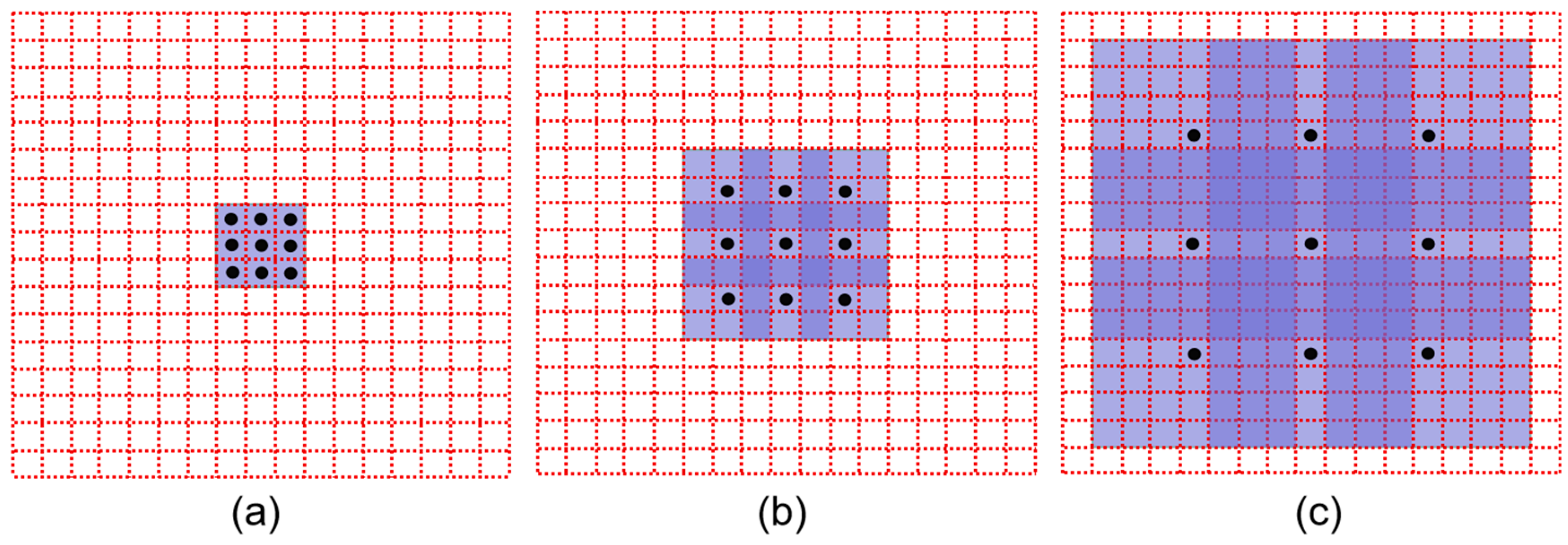
We use a set of pictures to illustrate the principle of dilated convolution. Figure 1a is the conventional convolution kernel, and the dilated convolution is obtained by adding intervals to this basic convolution kernel. Figure 1b corresponds to the convolution of 3 × 3, with dilation rate of 2 and interval 1, that is, corresponding to 7 × 7 image blocks. It can be understood that the kernel size becomes 7 × 7, but only 9 points have parameters, and the rest have parameters of 0. Convolution calculation was performed for the 9 points in Figure 1b and the corresponding pixels in the feature map, and the other positions were skipped. Figure 1b,c are similar, except that the dilation rate is 4, which is equivalent to a 15 × 15 convolution kernel. As the convolution kernel becomes larger, the receptive field becomes larger naturally.

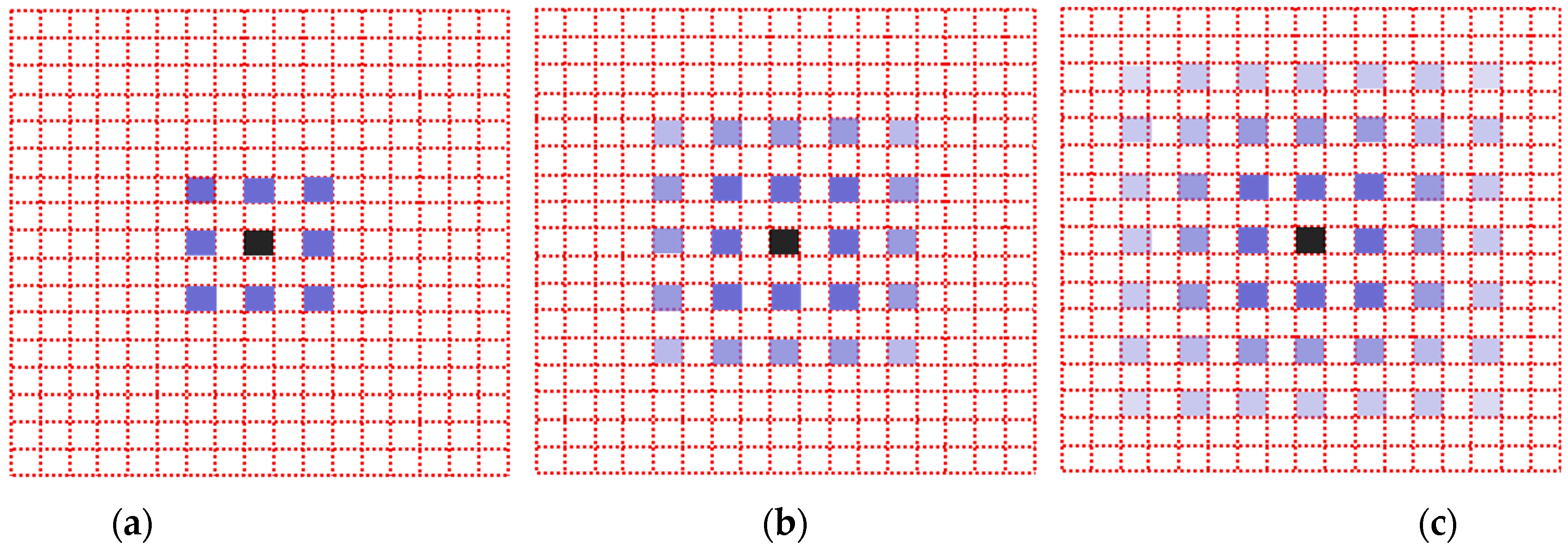
In practical application, when the same dilation rate is used for all convolutional layers, a problem called grid effect will appear. Since the convolution calculation points on the feature map are discontinuous, for example, if we repeatedly accumulate 3 × 3 kernel of dilation rate 2, this problem will occur.

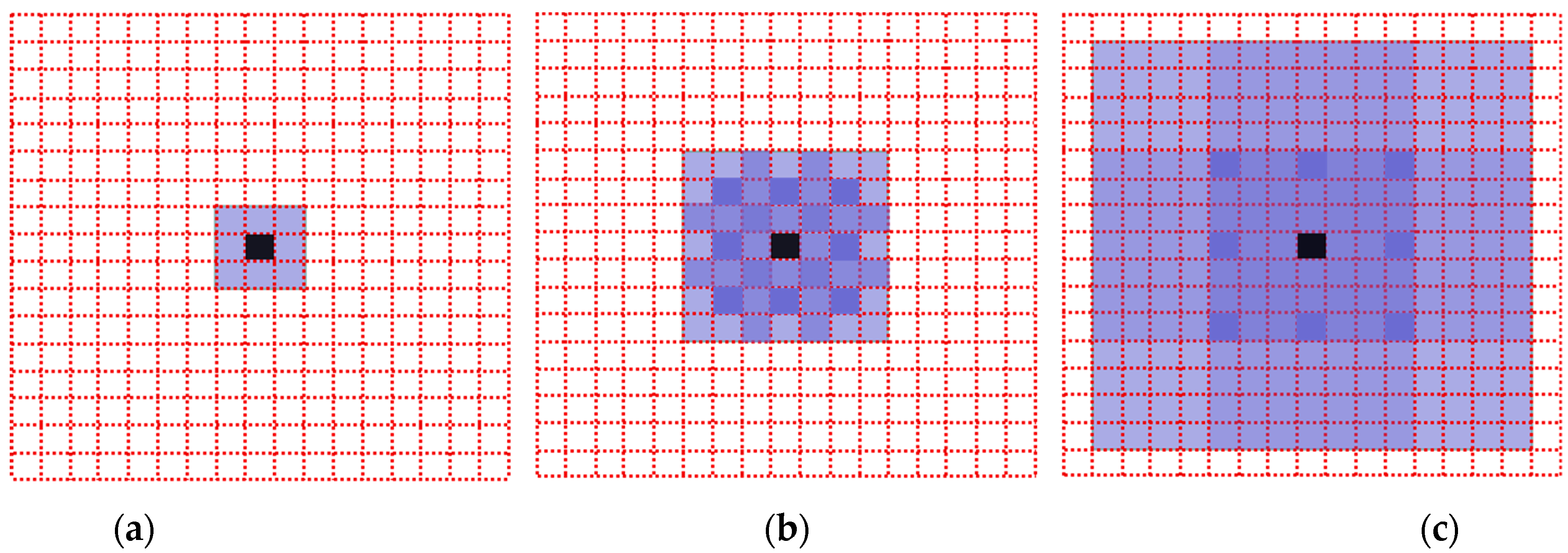
The blue square in Figure 2 is the convolution calculation points participating in the calculation, and the depth of the color represents the calculation times. As can be seen, since the dilation rates of the three convolutions are consistent, the calculation points of the convolution will show a grid expansion outward, while some points will not become calculation points. Such kernel discontinuities, that is, not all pixels are used for calculations, will result in the loss of continuity of information, which is very detrimental for tasks such as pixel-level dense prediction. The solution is to discontinuously use dilated convolution with the same dilation rate, but this is not comprehensive enough. If the dilation rate is multiple, such as 2,4,8, then the problem still exists. Therefore, the best way is to set the dilation rate of continuous dilated convolution as “jagged”, such as 1,2,3, respectively, so that the distribution of convolution calculation points will become like Figure 3 without discontinuity.

3. The Architecture of the Modified U-Net

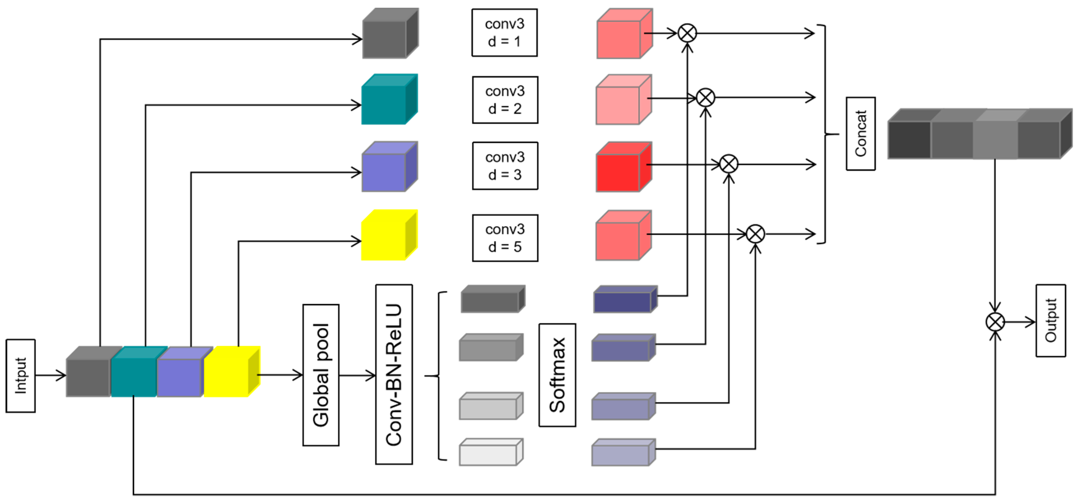
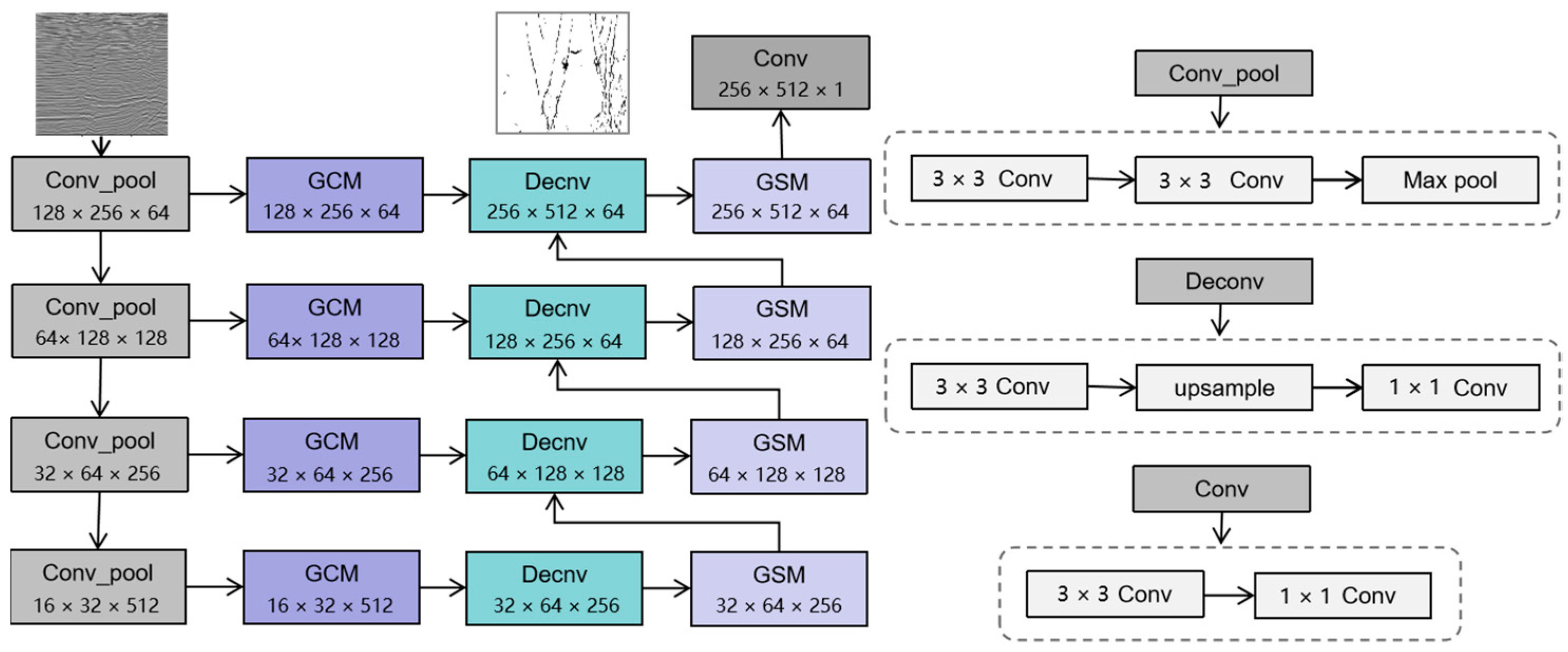
The proposed neural network adopts a U-Net of a 4-layer structure as the basic network. In the coding path, feature maps of each layer are connected to the corresponding decoding layer by GCM, in which each layer adopts two 3 × 3 convolution layers and maximum pooling layer for feature extraction. Then, in the decoding path, feature maps of each layer are connected to the corresponding decoding layer by GSM. Each layer adopts a 3 × 3 convolution layer, up-sampling layer and 1 × 1 convolution layer to restore, and the output layer adopts a 3 × 3 convolution layer and 1 × 1 convolution layer to output. In this modified U-Net, the batch regularization (BN) and modified linear units (ReLU) are added to all convolution layers to correct data distribution, except for the output layer. GCM and GSM modules play a key role in the modified U-Net, and their operation mechanism is similar. GCM module can divide the input feature map into four groups on average, and then carry out the dilated convolution operation with dilation rates of 1, 2, 3 and 5, respectively. In addition, the module extracts and outputs the features of the input feature map through pooling, convolution, batch regularization, activation, softmax and other conventional operations, and finally obtains the channel information of all groups. For the GSM module, it can divide the input feature map into three groups on average, and each group carries out the dilated convolution operation with dilation rates of 1, 2 and 4, respectively. This module carries out feature extraction and output in sequence by down-sampling, convolution, batch regularization, activation, up-sampling, convolution, batch regularization, activation and softmax, and finally obtains the spatial information of all groups.

Figure 4 shows the structure of GCM in the modified U-Net. This module divides the input feature map into four groups evenly, and each group performs dilated convolution operations with dilation rates of 1, 2, 3, and 5. The size of the target area of fault identification determines the value of the dilation rate. After dilated convolution, four groups of feature maps with different scales are obtained. Besides, four groups of channel information are returned by softmax, which were taken as weights and multiplied by four groups of feature maps with different scales obtained via dilated convolutions to acquire new feature maps. The receptive field corresponding to the group with the largest weight contributed the most to the final network prediction. Finally, the four groups of new feature maps are spliced together and then a residual operation is performed with the input feature map to obtain the final prediction result. The GCM module uses the idea of grouping and realizes the automatic selection of inter-group multi-scale information under the guidance of channel information.

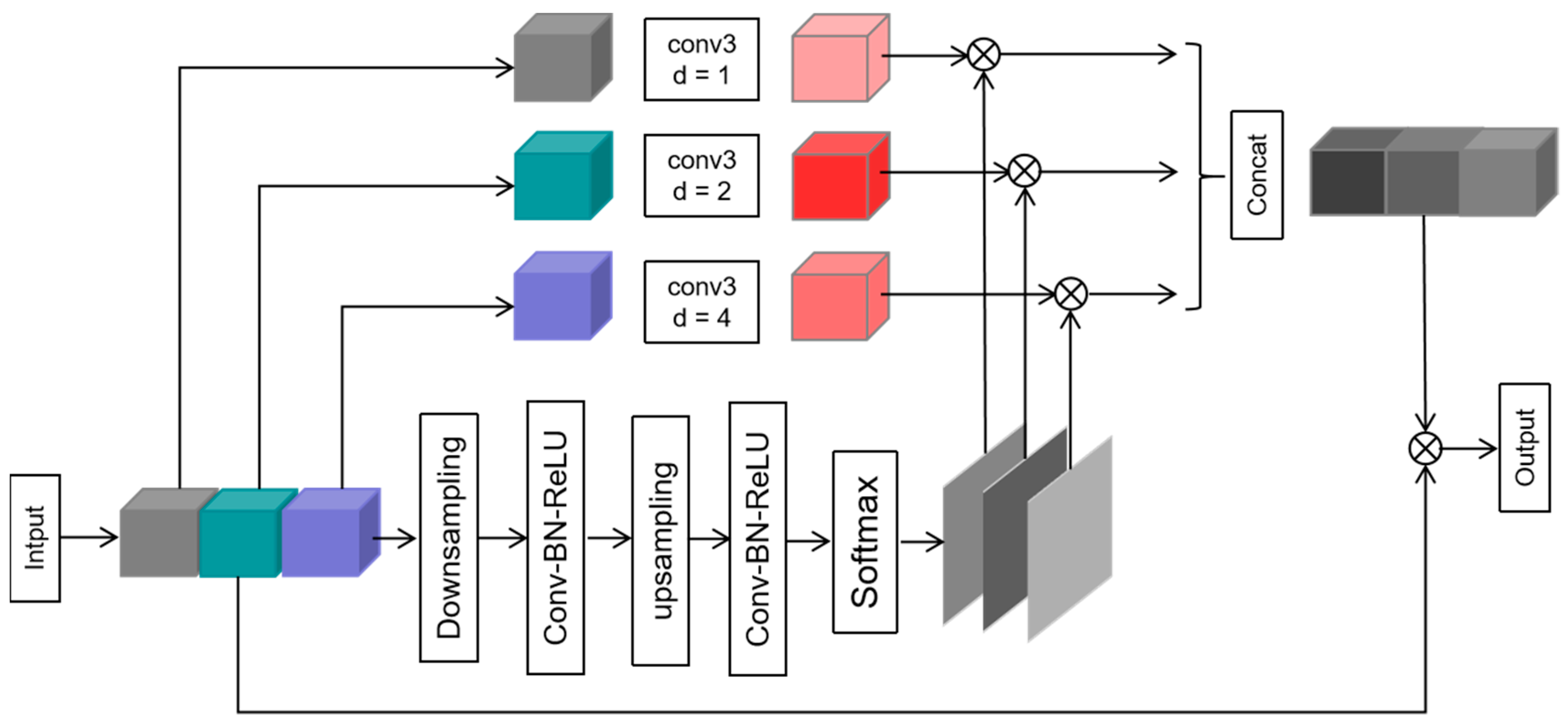
Figure 5 shows the structure of GSM, which realizes the selection of multi-scale information between groups in another way and enhances the consistency of receptive field and target region recognition. In this module, the input feature map was divided into three groups, and then three groups of feature maps with different scales are obtained by the dilated convolution with dilation rates of 1, 2 and 4. At the same time, three feature maps with spatial weights are cropped from the input feature map through a series of conventional operations. In these operations, the purpose of down-sampling is to obtain more global information, the purpose of up-sampling is to restore the size of feature maps, and the purpose of softmax is to enable the module to automatically select multi-scale information. Three feature maps with spatial weights are multiplied by three feature maps of different scales obtained by dilated convolution to get three new feature maps. Finally, after splicing the three groups of new feature maps, a residual operation is performed with the input feature map to acquire the final prediction results. In summary, under the guidance of spatial information, the GSM module can select multi-scale information among a group of feature maps.

The proposed neural network is based on the U-Net network and has two functional modules, the GCM and GSM, which can finely describe faults of different scales. Its architecture is shown in Figure 6. Due to the powerful multi-scale information selection ability of GCM and GSM modules, this paper only uses a 4-layer U-Net based on a coding–decoding structure as the basic network. In the coding path, only two 3 × 3 convolution and maximum pooling are used to quickly obtain feature maps with different resolutions. In the decoding path, multiple simple decoding blocks are used to quickly and effectively recover feature maps with high resolution. In this neural network, the data distribution after convolution is corrected by BN and ReLU, and the GCM module is placed at the connection layer of the network to automatically select multi-scale information, which makes up for the lack of transmitting single information to the decoder by the encoder of conventional U-Net. At the same time, the GSM module between groups is placed in the path of decoder to realize the function of multi-scale information selection, which makes up for the disadvantage of losing global information in up-sampling process.

4. Loss Function

The neural network will produce deviation between prediction and reality during training, and the deviation value is represented by loss function. During the training, the stochastic gradient descent (SGD) algorithm is used to update the network parameters and reduce the value of the loss function, so that the prediction and the actual convergence gradually, tend to be consistent [26]. The final result of neural network output is fault probability body, where 1 represents fault and 0 represents non-fault. In this study, fault recognition is regarded as a binary segmentation task. In the fault probability body, the most part is non-fault, and the least part (less than 10%) has a value of 1. There are strong data imbalance and uneven fault distribution area. In this case, the binary cross entropy loss (BCE) function is most often used [6,27]. Dice loss function is commonly used to serve the segmentation and recognition tasks of small-scale targets in medical research [28]. In this research, BCE and Dice are combined to solve problems such as data imbalance, uneven fault distribution area and insufficient accuracy in fault identification. The expression of the combined loss function is as follows:

$$\{\begin{array}{c}{L}_{BCE}=-\frac{1}{N}{\displaystyle \sum _i^N(g_i\log (p_i)+(1-g_i)\log (1-p_i))}\\ L_{Dice}=1-\frac{2{\displaystyle \sum _i^N{p}_i{g}_i+\epsilon }}{{\displaystyle \sum _i^N{p}_i}+{\displaystyle \sum _i^N{g}_i+\epsilon }}\\ L=\lambda L_{BCE}+L_{Dice}\end{array}$$

where N is the total number of pixels in the input image. $p_i\in \left[0,1\right]$ and $g_i\in \left[0,1\right]$ represent the prediction probability and label value of pixel, respectively, $\epsilon$ is the smoothing factor, whose value range is (0.1,1). $\lambda$ is the balance coefficient of Dice loss and BCE loss.

5. Training and Validation

In the neural network training, we randomly selected 1000 seismic images from an open-source dataset [15] for training, and the corresponding label data were also completed by manual marking in advance, marked as 1 in places with faults and 0 in places without faults. The purpose of network training is to optimize the parameters of the whole network. With each training, the deviation between the prediction and the actual represented by the loss function will decrease until the prediction and the actual tend to be consistent.

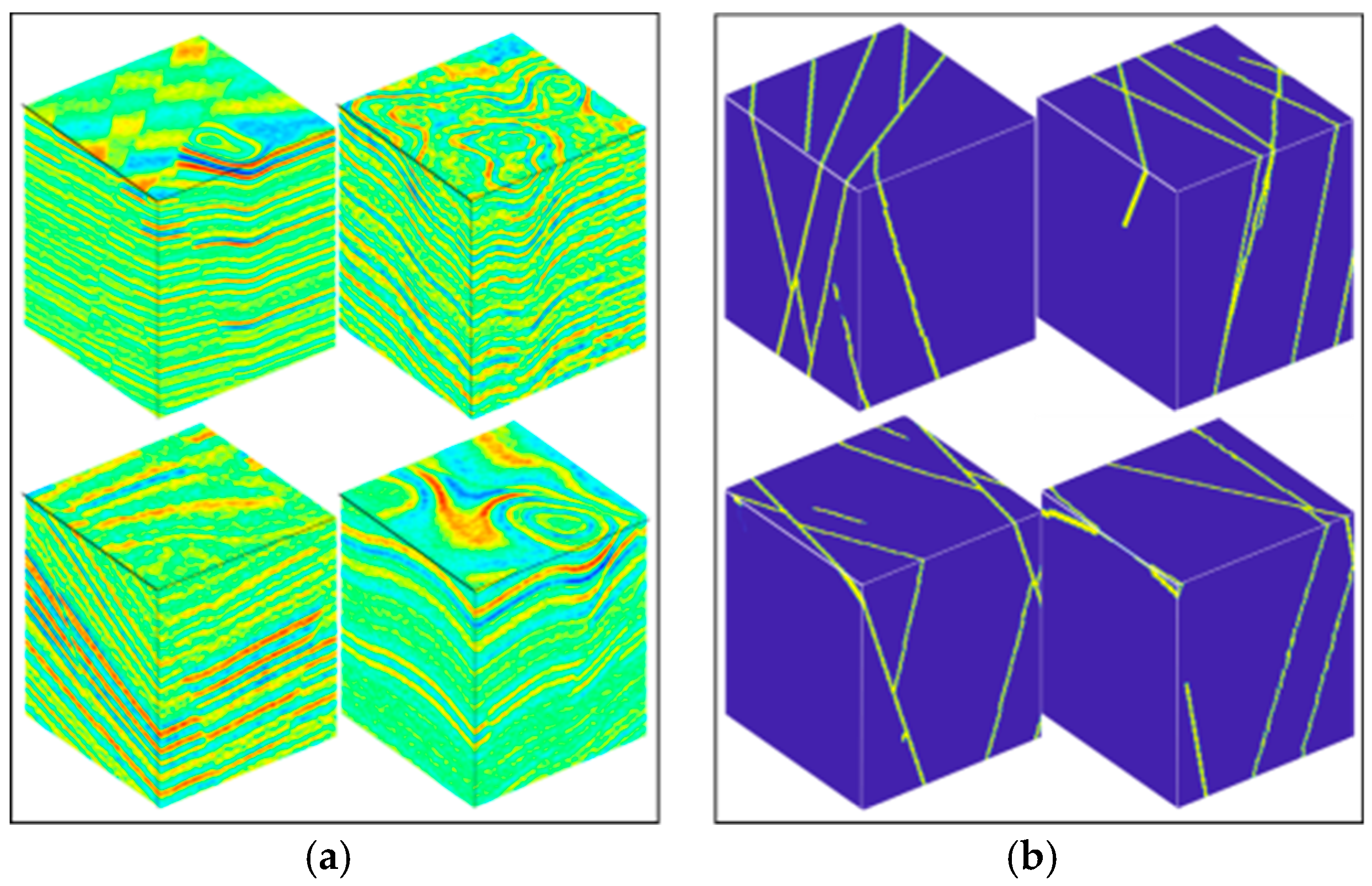
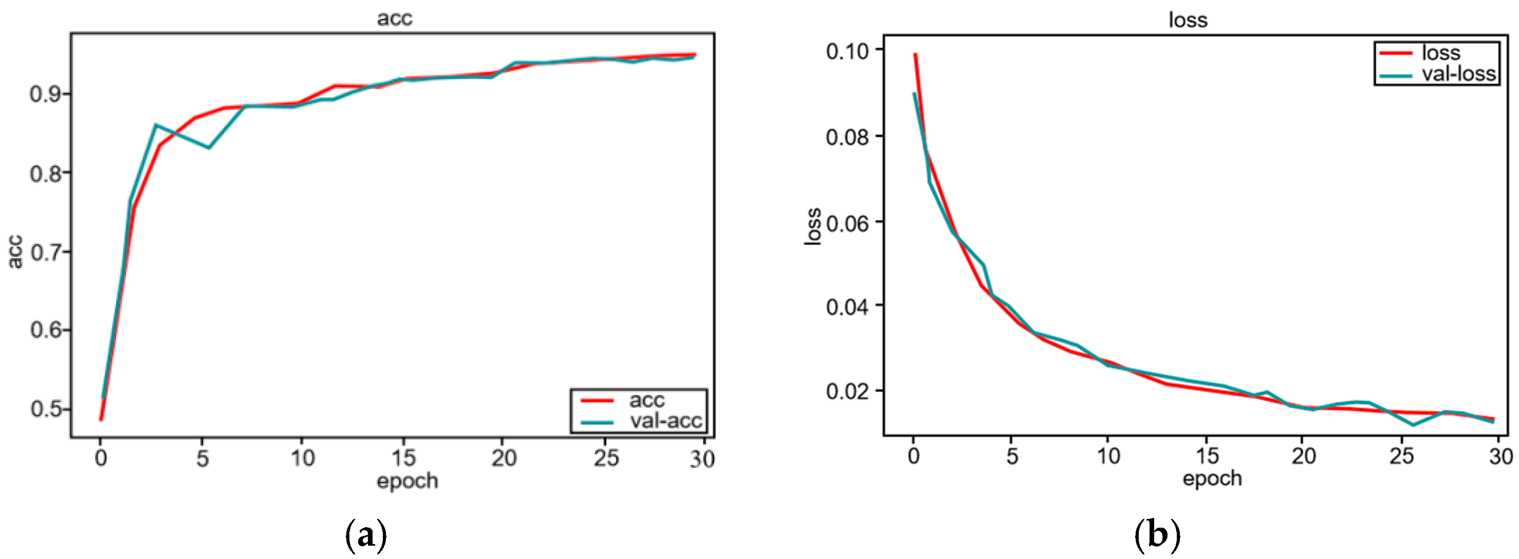
Figure 7 shows randomly seismic data sets with their corresponding labels. We used another 200 images as test and validation data, which were not included in the training. In the process of training, SGD is used to optimize the network, and the number of images sent into the network is 10 each time. The network model can be trained when the number of epochs reaches 30 times. Figure 8a shows the change of training accuracy and validation accuracy of the modified U-Net with the number of epochs. After 30 epochs, the accuracy rate tends to be above 0.9. Figure 8b shows the changes of training loss and validation loss of the modified U-Net with the number of epochs. After 30 epochs, the loss value tends to 0.01. After training, save the network parameters. In the process of training and validation, in order to increase the diversity of training data sets and make the trained neural network have better classification or recognition performance, data enhancement is used to improve the diversity of training data sets. The data enhancement operation mainly includes data reversal and rotation around the time axis.

6. Application

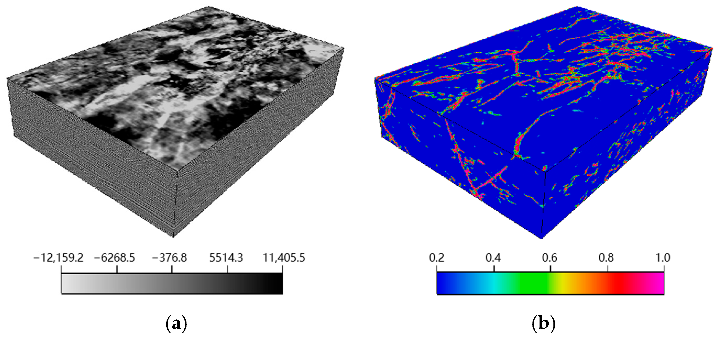
This paper used field data to verify the effectiveness of the trained network, and the fault probability volume is shown in Figure 9. In order to facilitate the interpretation of results, the opacity of the fault probability cube was adjusted and superimposed on the original seismic image. At the same time, we used a trained U-Net to identify faults of this data, and other parameters were completely the same except for GCM and GSM modules. The study area is located in a sandstone oil field in China, and the faults are mainly Y-shaped throughout the section and occur in almost every formation [29]. In the 700 ms–1500 ms time window, the number of faults is the largest, and the characteristics of faults are the most complex [30]. As depth increases, the imaging accuracy of seismic data decreases and the difficulty of fault imaging becomes more and more. On the plane, the fault is affected by the tension and strike-slip stress mechanism, and the fault direction is mainly NE and NW. This data set consists of 495 (lines) × 580 (CDPs) with a CDP spacing of 25 m and a line spacing of 25 m. The data are sampled at 1 ms with a length of 2 s. The inline number and xline number are in the range of (2410,2905) and (3600,4180), respectively. By using an NVIDIA TITAN Xp GPU, it takes about 110 min to calculate the fault probability volume. The randomly selected vertical profiles and time slice are inline 2510, xline 4025 and time slice at 1540 ms, respectively. The fault imaging results of the modified U-Net and U-Net are shown in Figure 10, Figure 11 and Figure 12.

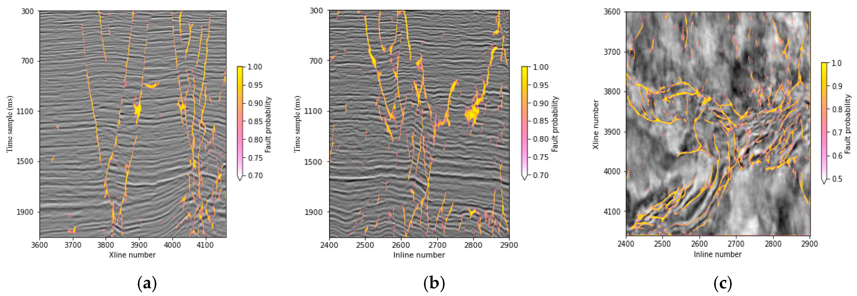
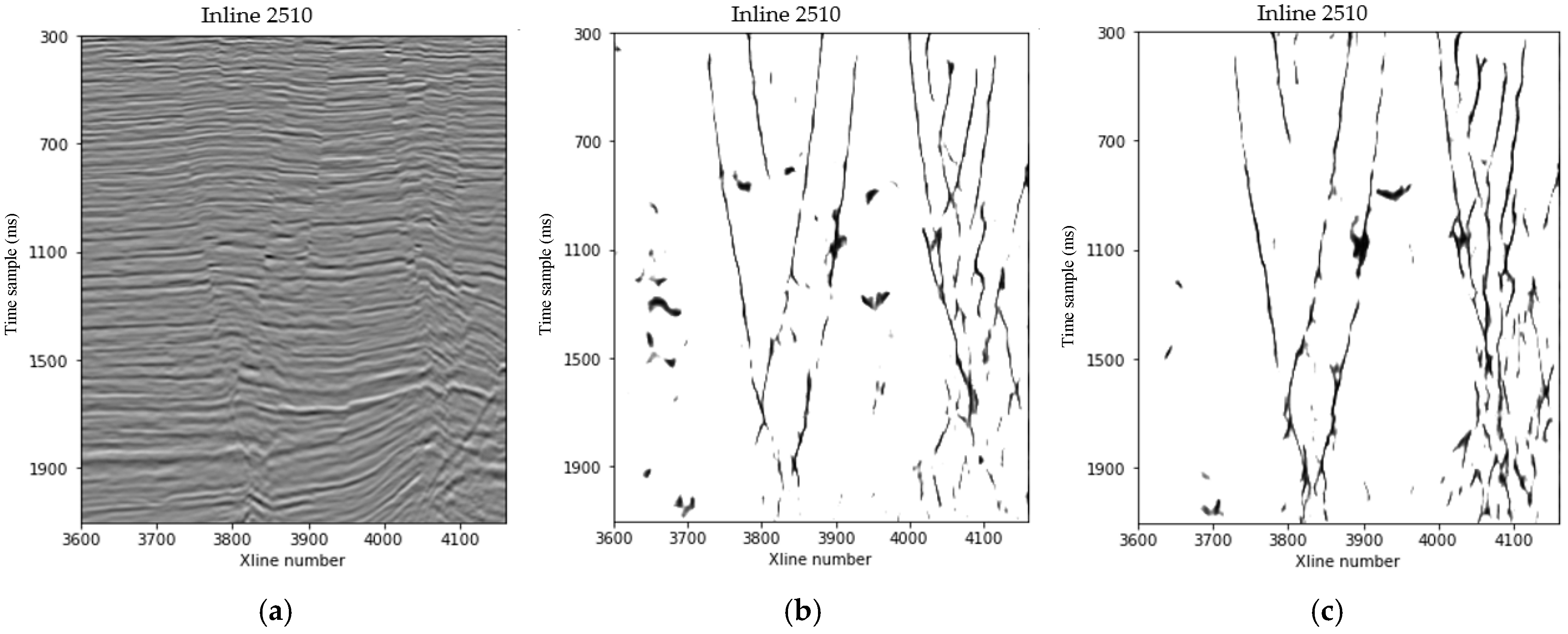
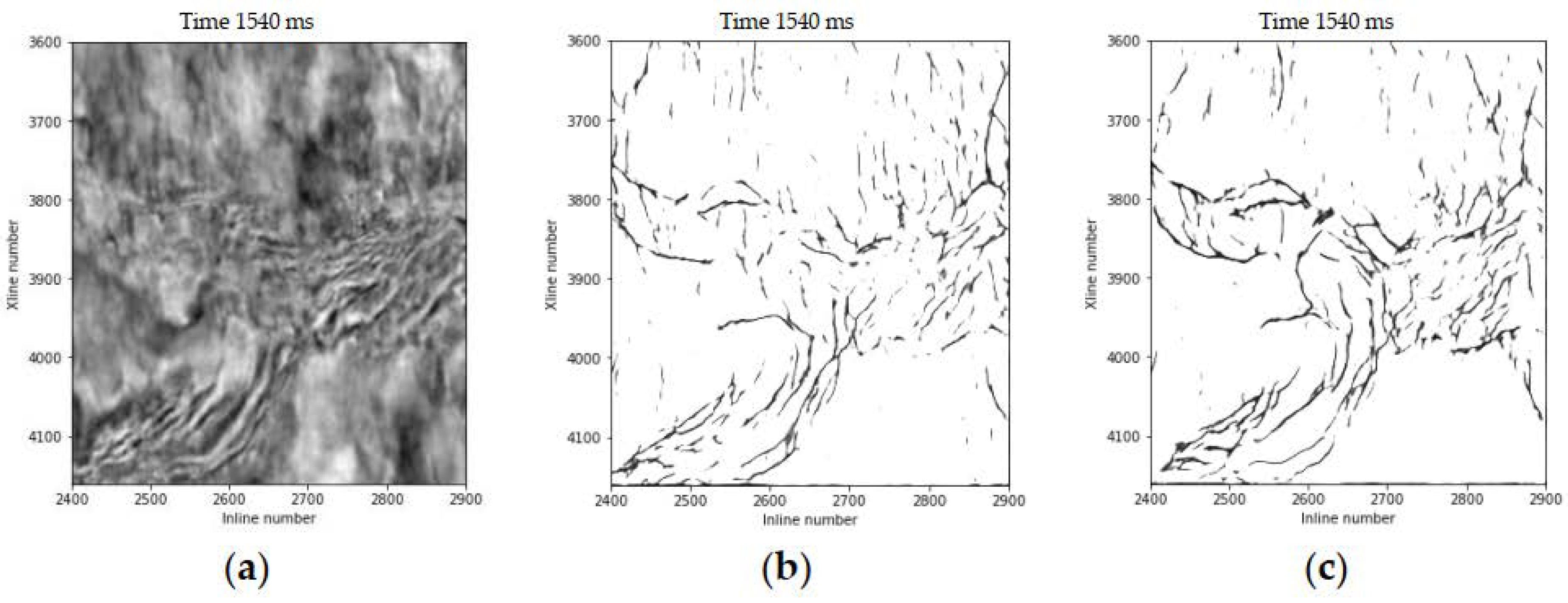
Figure 10 represents three seismic images in different directions with different scales faults that are imaged using the trained modified U-Net model. Figure 11b shows the fault image predicted by the trained U-Net model and Figure 11c shows the modified U-Net prediction results. The U-Net result (Figure 11b) is reliable enough to depict faults in this seismic image, however, much of the detail is still missing compared to features predicted by the modified U-Net (Figure 11c). Figure 12b,c illustrate fault imaging results of different slices. We observe that most faults can be clearly imaged under the trained modified U-Net model, and multiple groups of faults in different directions can be distinguished on horizontal slices. Figure 12b is the result of U-Net prediction, some small fracture information has not been portrayed. In summary, the field data example shows that the proposed method based on the modified U-Net has superior performance in detecting faults of multiple scales, and provides relatively high sensitivity and continuity.

7. Conclusions

We developed a modified U-Net-based method to automatically image faults in the sandstone reservoirs in China. The proposed network containing GCM and GSM modules is designed and trained to enhance the ability of the network to select multi-scale information. The GCM and GSM module can select multi-scale information obtained by convolution of different dilation rates between groups, enhance the consistency of receptive field and fault recognition target region, and jointly improve the recognition ability of micro-faults. The field data applications demonstrate the effectiveness of this approach. For sandstone oil and gas reservoirs in China with abundant faults, this method has great advantages in improving fault imaging accuracy, but further research is needed in improving computational efficiency and optimizing network architectures.

References

- Liu, B.; Sun, J.; Zhang, Y.; He, J.; Fu, X.; Yang, L.; Xing, J.; Zhao, X. Reservoir space and enrichment model of shale oil in the first member of Cretaceous Qingshankou Formation in the Changling sag, southern Songliao Basin, NE China. Pet. Explor. Dev. 2021, 48, 608–624. [Google Scholar] [CrossRef]
- Xu, J.; Zhang, L. Genesis of Cenozoic basins in Northwest Pacific Ocean margin (1): Comments on basin-forming mechanism. Oil Gas Geol. 2000, 21, 93–98. [Google Scholar]
- Chen, W.-C.; Yan, J.-J. On the Evolutional Characteristics of Cenozoic Episodic rifting of Nanpu Sag. J. Jining Norm. Coll. 2020, 3, 115–119. [Google Scholar]
- Peacock, D.C.P.; Sanderson, D.J.; Rotevatn, A. Relationships between fractures. J. Struct. Geol. 2018, 106, 41–53. [Google Scholar] [CrossRef]
- Tong, H.; Zhao, B.; Cao, Z.; Liu, G.; Dun, X.M.; Zhao, D. Structural analysis of faulting system origin in the Nanpu sag, Bohai Bay basin. Acta Geol. Sin. 2013, 87, 1647–1661. [Google Scholar]
- Wu, J.; Liu, B.; Zhang, H.; He, S.; Yang, Q. Fault Detection Based on Fully Convolutional networks (FCN). J. Mar. Sci. Eng. 2021, 9, 259. [Google Scholar] [CrossRef]
- LeCun, Y.; Bengio, Y.; Hinton, G. Deep learning. Nature 2015, 521, 436–444. [Google Scholar] [CrossRef] [PubMed]
- Smith, J.A. LAI Inversion Using a Back-propagation Neural Network Trained with a Multiple Scattering Model. IEEE Trans. Geosci. Remote Sens. 1993, 31, 1102–1106. [Google Scholar] [CrossRef] [Green Version]
- Krizhevsky, A.; Sutskever, I.; Hinton, G.E. ImageNet classification with deep convolutional neural networks. Commun. ACM 2017, 60, 84–90. [Google Scholar] [CrossRef]
- Zheng, Z.H.; Kavousi, P.; Di, H.B. Multi-Attributes and Neural network-Based Fault Detection in 3D Seismic Interpretation. Adv. Mater. Res. 2014, 838–841, 1497–1502. [Google Scholar] [CrossRef]
- Araya-Polo, M.; Dahlke, T.; Frogner, C.; Zhang, C.; Poggio, T.; Hohl, D. Automated fault detection without seismic processing. Lead. Edge 2017, 36, 208–214. [Google Scholar] [CrossRef]
- Waldeland, A.; Solberg, A. Salt classification using deep learning. In Proceedings of the 79th EAGE Conference and Exhibition 2017, Paris, France, 12–15 June 2017. [Google Scholar]
- Guitton, A.; Wang, H.; Trainor-Guitton, W. Statistical imaging of faults in 3D seismic volumes using a machine learning approach. In SEG Technical Program Expanded Abstracts; Society of Exploration Geophysicists: Tulsa, OK, USA, 2017; pp. 2045–2049. [Google Scholar]
- Xiong, W.; Ji, X.; Ma, Y.; Wang, Y.; AlBinHassan, N.M.; Ali, M.N.; Luo, Y. Seismic fault detection with convolutional neural network. Geophysics 2018, 83, 97–103. [Google Scholar] [CrossRef]
- Wu, X.; Liang, L.; Shi, Y.; Fomel, S. FaultSeg3D: Using synthetic data sets to train an endto-end convolutional neural network for 3D seismic fault segmentation. Geophysics 2019, 84, IM35–IM45. [Google Scholar] [CrossRef]
- Ronneberger, O.; Fischer, P.; Brox, T. U-Net: Convolutional networks for biomedical image segmentation. In Medical Image Computing and Computer-Assisted Intervention, Proceedings of the MICCAI 2015, Munich, Germany, 5–9 October 2015; Lecture Notes in Computer Science; Navab, N., Hornegger, J., Wells, W.M., Frangi, A.F., Eds.; Springer: Cham, Switzerland, 2015; Volume 9351, pp. 234–241. [Google Scholar]
- Sevastopolsky, A. Optic disc and cup segmentation methods for glaucoma detection with modification of U-Net convolutional neural network. Pattern Recognit. Image Anal. 2017, 27, 618–624. [Google Scholar] [CrossRef] [Green Version]
- Zhang, H.; Han, J.; Li, Z.; Zhang, H. Extracting Q Anomalies from Marine Reflection Seismic Data Using Deep Learning. IEEE Geosci. Remote Sens. Lett. 2021, 19, 7501205. [Google Scholar] [CrossRef]
- Liang, C.; Wang, N.; Zhu, M.; Yang, X.; Li, J.; Gao, X. Based on Multi-Scale Feature Fusion Faces—Sketch Synthesis. China Science, Information Science, 1–14. Available online: http://kns.cnki.net/kcms/detail/11.5846.TP.20220126.1627.002.html (accessed on 4 January 2022).
- Ma, L.; Liu, X.; Li, H.; Duan, J.; Niu, B. Neural Network Lightweight Method Using Cavity Convolution. Computer Engineering and Applications: 1–14. Available online: http://kns.cnki.net/kcms/detail/11.2127.TP.20210419.1339.035.html (accessed on 4 January 2022).
- Yu, Q.; Zhang, J.; Wei, X.; Zhang, Q. Segmentation of liver tumors based on cascated separable cavity residual U-NET. Chin. J. Appl. Sci. 2021, 39, 378–386. [Google Scholar]
- Fisher, Y.; Koltun, V. Multi-scale context aggregation by dilated convolutions. arXiv 2015, arXiv:1511.07122. [Google Scholar]
- Zhe, Z.; Bilin, W.; Zhezhou, Y.; Zhiyuan, L. Dilated Convolutional Pixels Affinity network for Weakly Supervised Semantic Segmentation. Chin. J. Electron. 2021, 30, 1120–1130. [Google Scholar] [CrossRef]
- Gao, H.; Cao, L.; Yu, D.; Xiong, X.; Cao, M. Semantic Segmentation of Marine Remote Sensing Based on a Cross Direction Attention Mechanism. IEEE Access 2020, 8, 142483–142494. [Google Scholar] [CrossRef]
- Meng, D.; Sun, L. Some New Trends of Deep Learning Research. Chin. J. Electron. 2019, 28, 1087–1091. [Google Scholar] [CrossRef]
- Rumelhart, D.E.; Hinton, G.E.; Williams, R.J. Learning representations by back-propagating errors. Nature 1986, 323, 533–536. [Google Scholar] [CrossRef]
- Xie, S.N.; Tu, Z.W. Holistically-Nested Edge Detection. In Proceedings of the International Conference on Computer Vision, Santiago, Chile, 7–13 December 2015; pp. 1395–1403. [Google Scholar] [CrossRef] [Green Version]
- Milletari, F.; Navab, N.; Ahmadi, S.A. V-Net: Fully Convolutional Neural networks for Volumetric Medical Image Segmentation. In Proceedings of the 2016 Fourth International Conference on 3D Vision (3DV), Stanford, CA, USA, 25–28 October 2016. [Google Scholar]
- Liu, B.; Zhao, X.; Fu, X.; Yuan, B.; Bai, L.; Zhang, Y.; Ostadhassan, M. Petrophysical characteristics and log identification of lacustrine shale lithofacies: A case study of the first member of Qingshankou Formation in the Songliao Basin, Northeast China. Interpretation 2020, 8, SL45–SL57. [Google Scholar] [CrossRef]
- Gao, D. Integrating 3D seismic curvature and curvature gradient attributes for fracture characterization:Methodologies and interpretational implications. Geophysics 2013, 78, O21–O31. [Google Scholar] [CrossRef]
Figure 1.
The dilated convolution with dilation rate of 1, 2 and 4, respectively. (a) dilation rate = 1; (b) dilation rate = 2; (c) dilation rate = 4.
Figure 2.
The dilated convolution with the same dilation rate of 2, respectively. There are grid effects in all three graphs. (a) the first convolution with dilation rate of 2; (b) the second convolution with dilation rate of 2; (c) the third convolution with dilation rate of 2.
Figure 3.
The dilated convolution with dilation rate of 1, 2 and 3, respectively. (a) dilation rate = 1; (b) dilation rate = 2; (c) dilation rate = 3.
Figure 4.
The architecture of GCM.
Figure 5.
The architecture of GSM.