Processing the Artificial Edge-Effects for Finite-Difference Frequency-Domain in Viscoelastic Anisotropic Formations

Abstract

Real sedimentary media can usually be characterized as transverse isotropy. To reveal wave propagation in the true models and improve the accuracy of migrations and evaluations, we investigated the algorithm of wavefield simulations in an anisotropic viscoelastic medium. The finite difference in the frequency domain (FDFD) has several advantages compared with that in the time domain, e.g., implementing multiple sources, multi-scaled inversion, and introducing attenuation. However, medium anisotropy will lead to the complexity of the wavefield in the calculation. The damping profile of the conventional absorption boundary is only defined in one single direction, which produces instability when the wavefields of strong anisotropy are reflected on that truncated boundary. We applied the multi-axis perfectly matched layer (M-PML) to the wavefield simulations in anisotropic viscoelastic media to overcome this issue, which defines the damping profiles along different axes. In the numerical examples, we simulated seismic wave propagation in three viscous anisotropic media and focused on the wave attenuation in the absorbing layers using time domain snapshots. The M-PML was more effective for wave absorption compared to the conventional perfectly matched layer (PML). In strongly anisotropic media, the PML became unstable, and prominent reflections appeared at truncated boundaries. In contrast, the M-PML remained stable and efficient in the same model. Finally, the modeling of the stratified cross-well model showed the applicability of this proposed algorithm to heterogeneous viscous anisotropic media. The numerical algorithm can analyze wave propagation in viscoelastic anisotropic media. It also provides a reliable forward operator for waveform inversion, wave equation travel-time inversion, and seismic migration in anisotropic viscoelastic media.

1. Introduction

Regarding the numerical modeling of wave propagation in anisotropic media, numerous studies have been implemented using finite difference and spectral methods in the time domain [1,2,3] to obtain the numerical solution in discrete geological media. These media may contain rocks with various properties, defined as acoustic, elastic, viscoelastic isotropic, and anisotropic. With the flourishing development of computational technology and numerical algorithms, wavefield simulation methods have played a crucial role in imaging subsurface characteristics. Various imaging methods, such as tomography [4,5], reverse time migration [6,7,8], and full-waveform inversion [9,10,11], require an efficient wavefield simulation method to generate synthetic waveform data to match the observed data.

Accurately performing wavefield modeling with high efficiency in complex media, which contains anisotropy and attenuation, is critical. In contrast to time-domain wavefield modeling, although it is challenging to solve the sparse linearized matrix, multi-source modeling can be performed efficiently, and attenuation can be easily introduced [12]. In addition, the physical parameters of the reservoir can be estimated by seismic inversion and imaging methods within a limited number of frequency components [13]. Operto et al. [14] developed frequency-domain finite-difference viscoacoustic wavefield modeling in tilted transversely isotropic (TTI) media. Jeong et al. [15] used the finite element method to simulate the frequency-domain wavefield of vertically transversely isotropic (VTI) media. Zhou et al. [16] implemented seismic wave modeling in elastic anisotropic media using the generalized stiffness reduction method. Yang et al. [17] developed a new version of the generalized stiffness reduction method for anisotropic media and incorporated it into the 2.5D spectral element method. Qiao et al. [3] derived attenuative anisotropic wave equations involving fractional time derivatives and solved them using the pseudospectral method. Reducing artificial reflections is still essential despite numerous frequency-domain modeling methods.

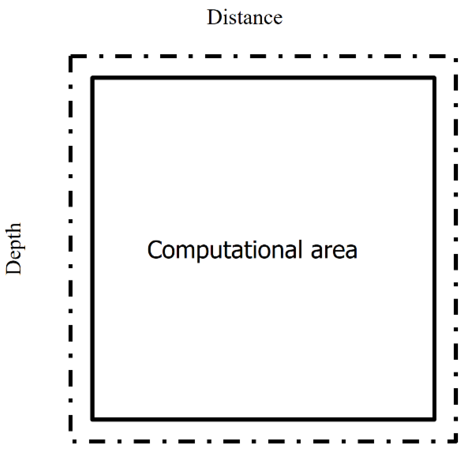
Figure 1 shows a sketch of the absorbing boundary condition (ABC). The middle area is the computational area, and the dashed-dot area is the truncated boundary. When the wavefield propagates to the boundary, the ABC needs to attenuate the reflections inwards. Since Berenger [18] developed a perfectly matched layer (PML) to reduce artificial reflections of the electromagnetic wavefield, many studies have shown success in its applications to acoustic and elastic wave modeling [19,20], and improvements have also been made to the perfectly matched layer method [21]. The PML method has become popular for wave modeling problems because it is applicable to first-order wave equations in the time domain [22] and frequency domain [23]. However, it is not straightforward how to implement it for second-order wave equations [24]. In addition, the most severe problem of PML may exist in absorbing artificial reflections in elastic anisotropic media. This is because PML can only function effectively when all slowness vector components of the waves are parallel to their corresponding group velocity vectors [25]. As is known, an elastic anisotropic wavefield generates multiple modes of waves and becomes more complex when the PML becomes unstable in dealing with the edge-effect problem. Thus, we need to replace PML in wavefield simulations of elastic anisotropic media.

A multi-axial perfectly matched layer (M-PML) boundary condition was developed in the time domain [26], and its stability has been verified in time-domain isotropic elastic modeling [27,28]. In this paper, the M-PML boundary condition is applied to frequency-domain finite-difference modeling in several elastic anisotropic media. The key point of this method is based on a more general version of coordinate stretching for PML, where waves are absorbed in all directions because the damping factor is specified in more than one direction. Then, by adjusting the proportion coefficients of the damping factors according to a specific model, M-PML can be stably performed. Comparing the wavefield generated in two homogenous media shows that PML, frequently used in the first-order wave equation, has the disadvantage of removing artificial reflections. At the same time, the M-PML performs well due to the damping profiles specified in multiple directions. Numerical experiments conducted in a strongly anisotropic medium show that M-PML remains stable in the frequency and time domains for viscoelastic anisotropic wavefield propagation. In addition, the M-PML requires only a modification of the damping factors. Therefore, the additional computational cost remains unchanged for techniques that rely on wavefield simulation, such as wave equation migration and waveform inversion.

2. Theoretical Foundations

2.1. Frequency Domain Elastic VTI Equation

The 2D frequency-domain anisotropic elastic Equation [10] is given as:

$$\begin{gathered} \rho {\omega }^2{u}_x+C_{11}\frac{{\partial }^2{u}_x}{\partial x^2}+C_{44}\frac{{\partial }^2{u}_x}{\partial z^2}+\left(C_{13}+C_{44}\right)\frac{{\partial }^2{u}_z}{\partial x\partial z}+f\left(\omega \right)=0, \\ \rho {\omega }^2{u}_z+C_{44}\frac{{\partial }^2{u}_z}{\partial x^2}+C_{33}\frac{{\partial }^2{u}_z}{\partial z^2}+\left(C_{13}+C_{44}\right)\frac{{\partial }^2{u}_x}{\partial x\partial z}+g\left(\omega \right)=0, \end{gathered}$$

(1)

where $\rho$ is the density, $f\left(\omega \right)$ and $g(\omega )$ are Fourier components of horizontal and vertical body forces, respectively; $u_x$ and $u_z$ are the horizontal and vertical displacements, respectively; and $\omega$ is the angular frequency. The elastic stiffness is written as:

$$\begin{array}{l}{C}_{11}=\left(1+2\epsilon \right)\rho v_{pr}^2,\\ C_{33}=\rho v_{pr}^2,\\ C_{13}=\sqrt{2\delta C_{33}\left(C_{33}-C_{44}\right)+{\left(C_{33}-C_{44}\right)}^2}-C_{44},\\ C_{44}=C_{55}=\rho v_{sr}^2,\end{array}$$

(2)

where $v_{pr}$ and $v_{sr}$ are the P-wave and the SV-wave velocity, respectively; $\epsilon$ and $\delta$ are Thomsen’s anisotropic parameters [29].

The frequency-domain finite-difference method can easily introduce attenuation [30]. The constant-Q model is adopted here, and the complex velocity is given as:

$$\begin{gathered} \frac{1}{v_p\left(\omega \right)}=\frac{1}{v_{pr}}\left(1-\frac{1}{\pi Q_p}\ln \left|\frac{\omega }{{\omega }_r}\right|\right)\cdot \left(1-\frac{\mathrm{i}}{2Q_p}\right), \\ \frac{1}{v_s\left(\omega \right)}=\frac{1}{v_{sr}}\left(1-\frac{1}{\pi Q_s}\ln \left|\frac{\omega }{{\omega }_r}\right|\right)\cdot \left(1-\frac{\mathrm{i}}{2Q_s}\right), \end{gathered}$$

(3)

where $v_p$, $v_s$ is the complex p-wave and SV-wave velocity, respectively; and $Q_p$, $Q_s$ is the quality factor of the P-wave and SV-wave; ${\omega }_r$ is the dominant frequency of the source wavelet; $i$ represents the imaginary unit. Substituting Equation (3) into Equation (2) yields the viscoelastic anisotropic wave equation.

2.2. Absorbing Boundary Condition

In order to introduce the M-PML absorbing condition to process unwanted reflections, the frequency-domain anisotropic elastic wave equation can be written as:

$$\begin{array}{l}\rho {\omega }^2{u}_x+\frac{1}{e_x}[C_{11}\frac{1}{e_x}\frac{{\partial }^2{u}_x}{\partial x^2}+C_{11}\frac{\partial }{\partial x}\left(\frac{1}{e_x}\right)\frac{\partial u_x}{\partial x}+C_{13}\frac{1}{e_z}\frac{{\partial }^2{u}_z}{\partial x\partial z}+C_{13}\frac{\partial }{\partial x}\left(\frac{1}{e_z}\right)\frac{\partial u_z}{\partial z}]\\ +\frac{1}{e_z}[C_{44}\frac{1}{e_x}\frac{{\partial }^2{u}_z}{\partial z\partial x}+C_{44}\frac{\partial }{\partial z}\left(\frac{1}{e_x}\right)\frac{\partial u_z}{\partial x}+C_{44}\frac{1}{e_z}\frac{{\partial }^2{u}_x}{\partial z^2}+C_{44}\frac{\partial }{\partial z}\left(\frac{1}{e_z}\right)\frac{\partial u_x}{\partial z}]+f\left(\omega \right)=0,\\ \rho {\omega }^2{u}_z+\frac{1}{e_x}[C_{44}\frac{1}{e_x}\frac{{\partial }^2{u}_z}{\partial x^2}+C_{44}\frac{\partial }{\partial x}\left(\frac{1}{e_x}\right)\frac{\partial u_z}{\partial x}+C_{44}\frac{1}{e_z}\frac{{\partial }^2{u}_x}{\partial x\partial z}+C_{44}\frac{\partial }{\partial x}\left(\frac{1}{e_z}\right)\frac{\partial u_x}{\partial z}]\\ +\frac{1}{e_z}[C_{13}\frac{1}{e_x}\frac{{\partial }^2{u}_x}{\partial z\partial x}+C_{13}\frac{\partial }{\partial z}\left(\frac{1}{e_x}\right)\frac{\partial u_x}{\partial x}+C_{33}\frac{1}{e_z}\frac{{\partial }^2{u}_z}{\partial z^2}+C_{33}\frac{\partial }{\partial z}\left(\frac{1}{e_z}\right)\frac{\partial u_z}{\partial z}]+g\left(\omega \right)=0,\end{array}$$

(4)

where $e_x=1-\mathrm{i}\frac{d_x\left(x\right)}{\omega }$ and $e_z=1-\mathrm{i}\frac{d_z\left(z\right)}{\omega }$, $x$ and $z$ are respectively the distance from the inner boundary of the horizontal and vertical direction; $d_x\left(x\right)$ is the damping profiles, given as:

$$d_x\left(x\right)=2\pi {\alpha }_0{f}_0\left(\frac{x}{L}\right),$$

(5)

where $x$ is the distance from the inner boundary of the horizontal direction; ${\alpha }_0$ is the optimized parameter, and here ${\alpha }_0$ is given as 1.79 [30]; $f_0$ is the dominant frequency of the source wavelet and $L$ is the thickness of the PML absorbing boundary condition. The new vertical coordinate has a similar form to the horizontal one:

$$d_z\left(z\right)=2\pi {\alpha }_0{f}_0\left(\frac{z}{L}\right),$$

(6)

where $z$ is the distance from the inner boundary of the vertical direction.

Artificial boundary reflection can seriously affect the effect of numerical modeling. Therefore, a frequency-domain multi-axial perfectly matched layer (M-PML) is exploited to absorb the unwanted reflections.

In classical PML, unwanted waves are only attenuated in one direction (uniaxial). Within the left and right boundaries, only the damping function along the x-direction is nonzero and can be formulated as:

$$d_x=d_x^x\left(x\right),d_z=0.$$

(7)

Similarly, within the bottom and left boundaries, only the damping function along the z-direction takes effect and can be given as:

$$d_x=0,d_z=d_z^z\left(z\right).$$

(8)

To attenuate unwanted reflections efficiently, M-PML was developed [26]. The basic idea of M-PML is that the damping functions are proportional to each other. The damping function along the x-direction can be defined as:

$$d_x=d_x^x\left(x\right),d_z=p^{\left(z/x\right)}{d}_x^x\left(x\right),$$

(9)

where $p^{\left(z/x\right)}$ is the proportion coefficient in either the right or left PML boundary.

Similarly, the damping function along the z-direction can be written as:

$$d_x=p^{\left(x/z\right)}{d}_z^z\left(z\right),d_z=d_z^z\left(z\right),$$

(10)

where $p^{\left(x/z\right)}$ is the proportion coefficient in either the bottom or top PML boundary. During implementation, the proportions $p^{\left(x/z\right)}$ are between 0 and 1 [27].

2.3. Numerical Implementation

Introducing the finite differences and derivatives can be summarized as follows:

$$\begin{gathered} \frac{\partial u_x}{\partial x}\approx \frac{1}{2\mathrm{\Delta }x}\left[u_x^{i+1,j}-u_x^{i-1,j}\right], \\ \frac{\partial u_x}{\partial z}\approx \frac{1}{2\mathrm{\Delta }z}\left[u_x^{i,j+1}-u_x^{i,j-1}\right], \\ \frac{{\partial }^2{u}_x}{\partial x^2}\approx \frac{1}{\mathrm{\Delta }{x}^2}\left[u_x^{i+1,j}-2u_x^{i,j}+u_x^{i-1,j}\right], \\ \frac{{\partial }^2{u}_x}{\partial z^2}\approx \frac{1}{\mathrm{\Delta }{z}^2}\left[u_x^{i,j+1}-2u_x^{i,j}+u_x^{i,j-1}\right], \\ \frac{{\partial }^2{u}_x}{\partial x\partial z}\approx \frac{1}{4\mathrm{\Delta }x\mathrm{\Delta }z}\left[u_x^{i+1,j+1}-u_x^{i+1,j-1}-u_x^{i-1,j+1}+u_x^{i-1,j-1}\right], \end{gathered}$$

(11)

where $\mathrm{\Delta }x$ and $\mathrm{\Delta }z$ are the horizontal and vertical grid sizes, respectively; and the value of grid sizes must be small enough so that there are enough grid points per wavelength [10]; $i$ and $j$ are the indices of the horizontal and vertical grids. The finite differences of $u_z$ are similar to the way of the horizontal one.

Using the finite-difference star stencil [10]:

$$\begin{array}{ccc}{M}_1& M_4& M_7\\ M_2& M_5& M_8\\ M_3& M_6& M_9\end{array}.$$

(12)

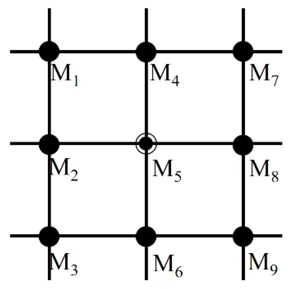
Substituting the finite difference of derivatives and each grid point of Equation (12) according to Figure 2 can be collected as follows:

$$\begin{gathered} M_1=\frac{{\left(C_{13}+C_{44}\right)}_{i,j}}{4\mathrm{\Delta }x\mathrm{\Delta }z{\left(e_x{e}_z\right)}_{i,j}}\left[\begin{array}{cc}0& 1\\ 1& 0\end{array}\right], \\ {M}_2=\left[\begin{array}{cc}\frac{{\left(C_{11}\right)}_{i,j}}{{\left(\mathrm{\Delta }x{\left(e_x\right)}_{i,j}\right)}^2}+\frac{{\left(C_{11}\right)}_{i,j}}{2\mathrm{\Delta }x{\left(e_x\right)}_{i,j}^3}\cdot \frac{\partial {\left(e_x\right)}_{i,j}}{\partial x}& \frac{{\left(C_{44}\right)}_{i,j}}{2\mathrm{\Delta }x{\left(e_z{e}_x^2\right)}_{i,j}}\cdot \frac{\partial {\left(e_x\right)}_{i,j}}{\partial z}\\ \frac{{\left(C_{13}\right)}_{i,j}}{2\mathrm{\Delta }x{\left(e_z{e}_x^2\right)}_{i,j}}\cdot \frac{\partial {\left(e_x\right)}_{i,j}}{\partial z}& \frac{{\left(C_{44}\right)}_{i,j}}{{\left({\left(e_x\right)}_{i,j}\mathrm{\Delta }x\right)}^2}+\frac{{\left(C_{44}\right)}_{i,j}}{2\mathrm{\Delta }x{\left(e_x\right)}_{i,j}^3}\cdot \frac{\partial {\left(e_x\right)}_{i,j}}{\partial x}\end{array}\right], \\ {M}_3=\frac{-{\left(C_{13}+C_{44}\right)}_{i,j}}{4\mathrm{\Delta }x\mathrm{\Delta }z{\left(e_x{e}_z\right)}_{i,j}}\left[\begin{array}{cc}0& 1\\ 1& 0\end{array}\right], \\ {M}_4=\left[\begin{array}{cc}\frac{{\left(C_{44}\right)}_{i,j}}{{\left(\mathrm{\Delta }z{\left(e_z\right)}_{i,j}\right)}^2}+\frac{{\left(C_{44}\right)}_{i,j}}{2\mathrm{\Delta }z{\left(e_z\right)}_{i,j}^3}\cdot \frac{\partial {\left(e_z\right)}_{i,j}}{\partial z}& \frac{{\left(C_{13}\right)}_{i,j}}{2\mathrm{\Delta }z{\left(e_x{e}_z^2\right)}_{i,j}}\cdot \frac{\partial {\left(e_z\right)}_{i,j}}{\partial x}\\ \frac{{\left(C_{44}\right)}_{i,j}}{2\mathrm{\Delta }z{\left(e_x{e}_z^2\right)}_{i,j}}\cdot \frac{\partial {\left(e_z\right)}_{i,j}}{\partial x}& \frac{{\left(C_{33}\right)}_{i,j}}{{\left({\left(e_z\right)}_{i,j}\mathrm{\Delta }z\right)}^2}+\frac{{\left(C_{33}\right)}_{i,j}}{2\mathrm{\Delta }z{\left(e_z\right)}_{i,j}^3}\cdot \frac{\partial {\left(e_z\right)}_{i,j}}{\partial z}\end{array}\right], \\ {M}_5=\left[\begin{array}{cc}{\omega }^2{\rho }_{i,j}-\frac{2{\left(C_{11}\right)}_{i,j}}{{\left(\mathrm{\Delta }x{\left(e_x\right)}_{i,j}\right)}^2}-\frac{2{\left(C_{44}\right)}_{i,j}}{{\left(\mathrm{\Delta }z{\left(e_z\right)}_{i,j}\right)}^2}& 0\\ 0& {\omega }^2{\rho }_{i,j}-\frac{2{\left(C_{44}\right)}_{i,j}}{{\left(\mathrm{\Delta }x{\left(e_x\right)}_{i,j}\right)}^2}-\frac{2{\left(C_{33}\right)}_{i,j}}{{\left(\mathrm{\Delta }z{\left(e_z\right)}_{i,j}\right)}^2}\end{array}\right], \\ {M}_6=\left[\begin{array}{cc}\frac{{\left(C_{44}\right)}_{i,j}}{{\left(\mathrm{\Delta }z{\left(e_z\right)}_{i,j}\right)}^2}-\frac{{\left(C_{44}\right)}_{i,j}}{2\mathrm{\Delta }z{\left(e_z\right)}_{i,j}^3}\cdot \frac{\partial {\left(e_z\right)}_{i,j}}{\partial z}& \frac{-{\left(C_{13}\right)}_{i,j}}{2\mathrm{\Delta }z{\left(e_x{e}_z^2\right)}_{i,j}}\cdot \frac{\partial {\left(e_z\right)}_{i,j}}{\partial x}\\ \frac{-{\left(C_{44}\right)}_{i,j}}{2\mathrm{\Delta }z{\left(e_x{e}_z^2\right)}_{i,j}}\cdot \frac{\partial {\left(e_z\right)}_{i,j}}{\partial x}& \frac{{\left(C_{33}\right)}_{i,j}}{{\left({\left(e_z\right)}_{i,j}\mathrm{\Delta }z\right)}^2}-\frac{{\left(C_{33}\right)}_{i,j}}{2\mathrm{\Delta }z{\left(e_z\right)}_{i,j}^3}\cdot \frac{\partial {\left(e_z\right)}_{i,j}}{\partial z}\end{array}\right], \\ {M}_7=\frac{-{\left(C_{13}+C_{44}\right)}_{i,j}}{4\mathrm{\Delta }x\mathrm{\Delta }z{\left(e_x{e}_z\right)}_{i,j}}\left[\begin{array}{cc}0& 1\\ 1& 0\end{array}\right], \\ {M}_8=\left[\begin{array}{cc}\frac{{\left(C_{11}\right)}_{i,j}}{{\left(\mathrm{\Delta }x{\left(e_x\right)}_{i,j}\right)}^2}-\frac{{\left(C_{11}\right)}_{i,j}}{2\mathrm{\Delta }x{\left(e_x\right)}_{i,j}^3}\cdot \frac{\partial {\left(e_x\right)}_{i,j}}{\partial x}& \frac{-{\left(C_{44}\right)}_{i,j}}{2\mathrm{\Delta }x{\left(e_z{e}_x^2\right)}_{i,j}}\cdot \frac{\partial {\left(e_x\right)}_{i,j}}{\partial z}\\ \frac{-{\left(C_{13}\right)}_{i,j}}{2\mathrm{\Delta }x{\left(e_z{e}_x^2\right)}_{i,j}}\cdot \frac{\partial {\left(e_x\right)}_{i,j}}{\partial z}& \frac{{\left(C_{44}\right)}_{i,j}}{{\left({\left(e_x\right)}_{i,j}\mathrm{\Delta }x\right)}^2}-\frac{{\left(C_{44}\right)}_{i,j}}{2\mathrm{\Delta }x{\left(e_x\right)}_{i,j}^3}\cdot \frac{\partial {\left(e_x\right)}_{i,j}}{\partial x}\end{array}\right], \\ {M}_9=\frac{{\left(C_{13}+C_{44}\right)}_{i,j}}{4\mathrm{\Delta }x\mathrm{\Delta }z{\left(e_x{e}_z\right)}_{i,j}}\left[\begin{array}{cc}0& 1\\ 1& 0\end{array}\right]. \end{gathered}$$

(13)

After using the finite difference method in the frequency domain, the final equation can be written as Equation (14). Thus, for each frequency component, the matrix equation can be given as:

$$M\left(\omega \right)U\left(\omega \right)=F\left(\omega \right).$$

(14)

The impedance matrix $M\left(\omega \right)$ can be obtained by Equation (13), $U\left(\omega \right)$ is the monochromatic wavefield, and $F\left(\omega \right)$ is the source term. The frequency-domain Ricker wavelet is used in the following numerical examples, and LU decomposition is used to solve the matrix Equation (14) to get the monochromatic wavefield.

3. Synthetic Examples

3.1. Comparative Analysis of the Stability of PML and M-PML

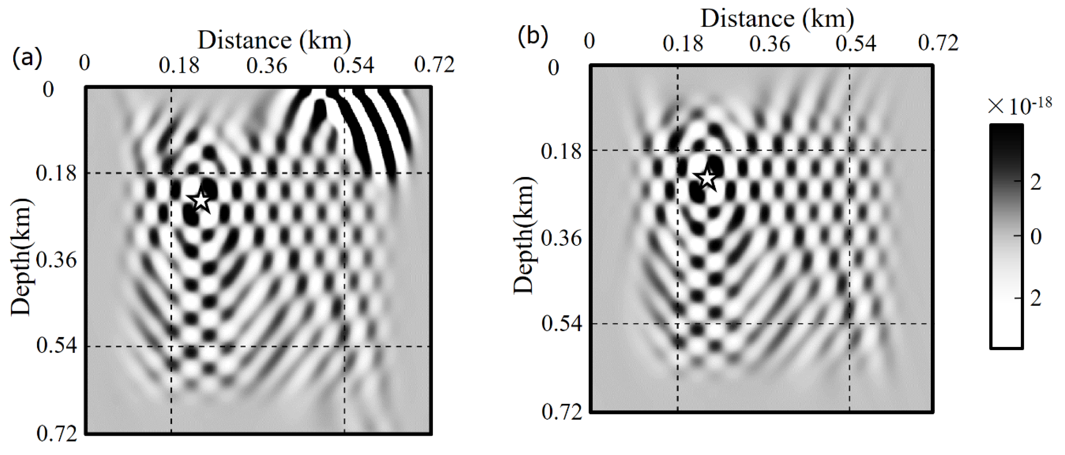
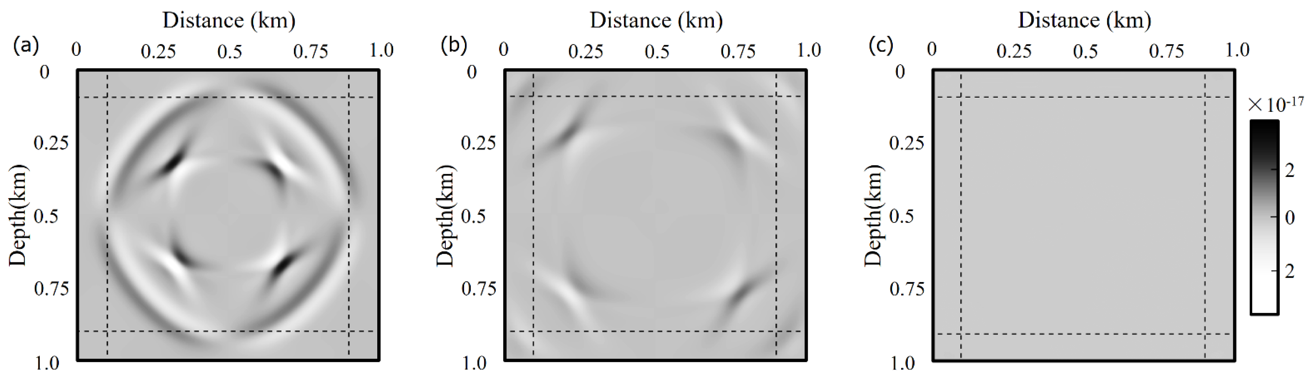
In this section, a medium of strong anisotropy was employed to test the stability and performance of PML and M-PML. The material properties of the strongly anisotropic medium are given in

Table 1. Model parameters used for numerical experiments.

Medium	Density (kg/m3)	Qp	Qs	Elastic Moduli (GPa)
Medium 1	3200	20	10	$\begin{array}{l}{C}_{11}=16.70;C_{13}=6.60;\\ C_{33}=14.00;C_{44}=6.63.\end{array}$
Medium 2	8900	20	10	$\begin{array}{l}{C}_{11}=30.70;C_{13}=10.3;\\ C_{33}=35.80;C_{44}=7.55.\end{array}$
Medium 3	1000	—	—	$\begin{array}{l}{C}_{11}=4.000;C_{13}=7.50;\\ C_{33}=20.00;C_{44}=2.00.\end{array}$

: medium 3. We performed wavefield simulations to test the instability of the boundary conditions and confirmed that M-PML outperformed PML in this strongly anisotropic medium. A square model was considered embedded in an absorbing boundary of four sides. The computational model of medium 3, similar to the model used in Meza-Fajardo [25], has a size of $720\mathrm{m}\times 720\mathrm{m}$, and it is discretized by $480\times 480$ grids with a grid size of 1.5 m. A boundary with a thickness of 120 grids is considered to observe the phenomenon of wave propagating inside truncated boundary conditions. A vertical source dominated by 15 Hz is located at the grid point $\left(230\mathrm{m},230\mathrm{m}\right)$, which is close to the artificial edge. The real parts of the monochromatic wavefields using classical PML and M-PML, respectively, are given in Figure 3. In Figure 3, the monochromatic wavefield at 15 Hz was calculated using classical PML and M-PML, respectively. The asterisk in Figure 3 and Figure 4 is the vertical source. The black dashed line in the figure shows the onset of the absorbing zone. From the results, it can be seen that the PML appears unstable at the boundary intersection in the upper right corner. This phenomenon is due to the complexity of the wavefield in the absorption boundary region, which leads to numerical instability of the PML. Since the PML is a uniaxially defined damping profile, absorption incompleteness is also observed in the other three corners. In the M-PML, however, since the damping profile is multi-axial, the instability that appears in the upper right corner of the PML is well resolved, and the attenuation of the waves is better in the corner regions.

Snapshots of the time-domain wavefield corresponding to Figure 3 are given in Figure 4. The black dashed line in Figure 4 is the onset of the absorbing boundary condition, and the source is indicated by an asterisk. Figure 4a,c,e,g are the wavefields calculated by PML, and Figure 4b,d,f,h are the wavefields calculated by M-PML. The results show that the PML-calculated wavefields display a significant instability because at 0.0818 s, the wavefield has not yet propagated to the boundary, but strong energy reflections have already occurred, and these reflections result from the instability remain almost constant as the wavefield propagates. Therefore, PML is unstable in strongly anisotropic media. In contrast, the results of M-PML in the right panel have no unstable reflections, and the waves are successfully absorbed in the truncated boundary regions, so the M-PML with multi-axial damping profiles solves the problem of instability of PML in strongly anisotropic media.

3.2. Comparative Analysis in Homogeneous Elastic Anisotropic Media

In the previous section, we verified that M-PML is superior to PML in terms of stability. However, the absorption performance advantages of M-PML and PML were not compared. Therefore, in this section, wavefield simulations are performed using M-PML and PML in different anisotropic media to compare the absorption of the two boundary conditions by observing the time-domain wavefield snapshots and comparing the energy curves. The energy of the wavefield snapshot is the sum of the squares of the amplitude values of each point in the wavefield. Then, the energy decay curve is obtained for each moment of the wavefield snapshot and plotted as a curve with the horizontal axis of time and the vertical axis of amplitude.

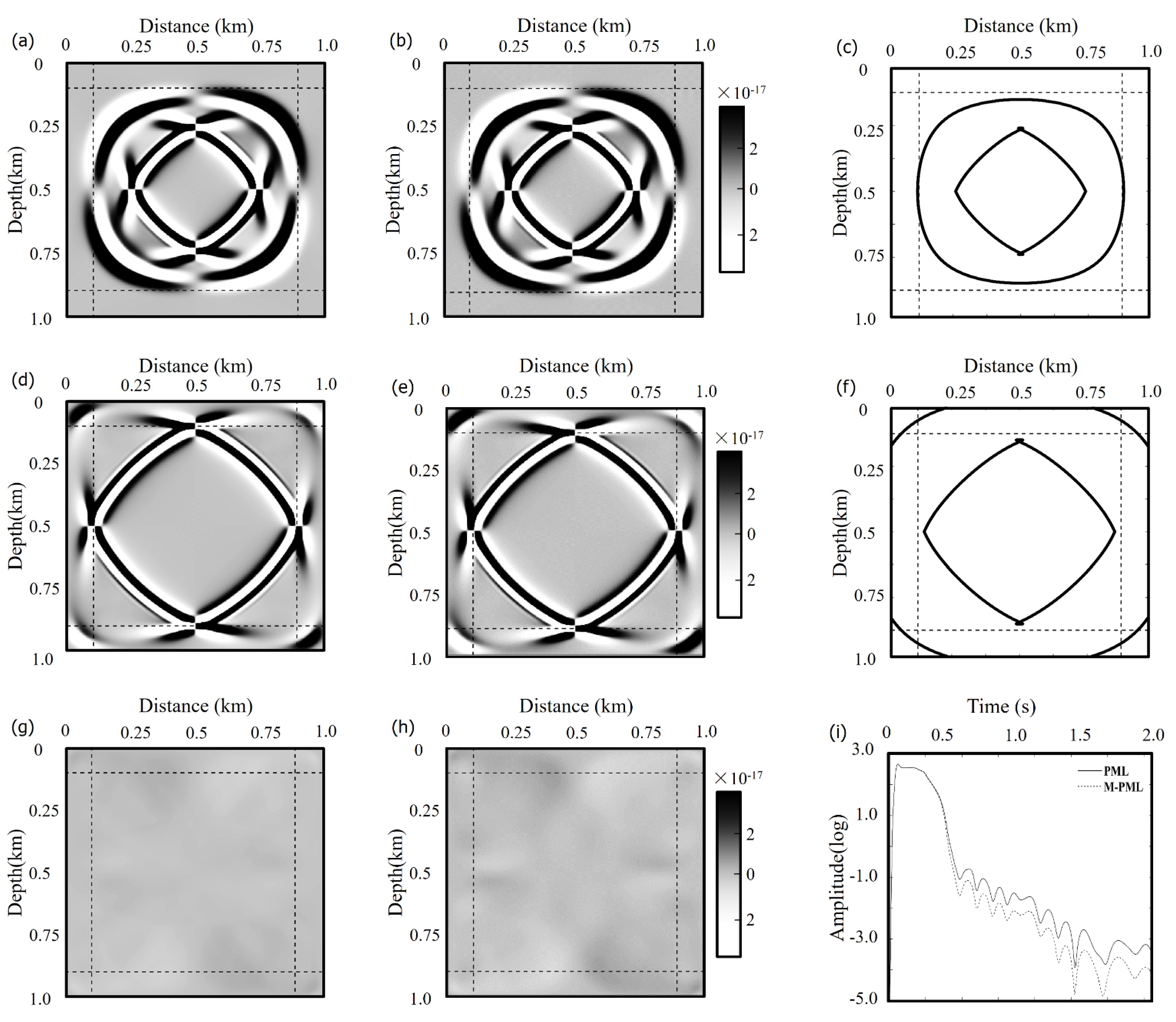
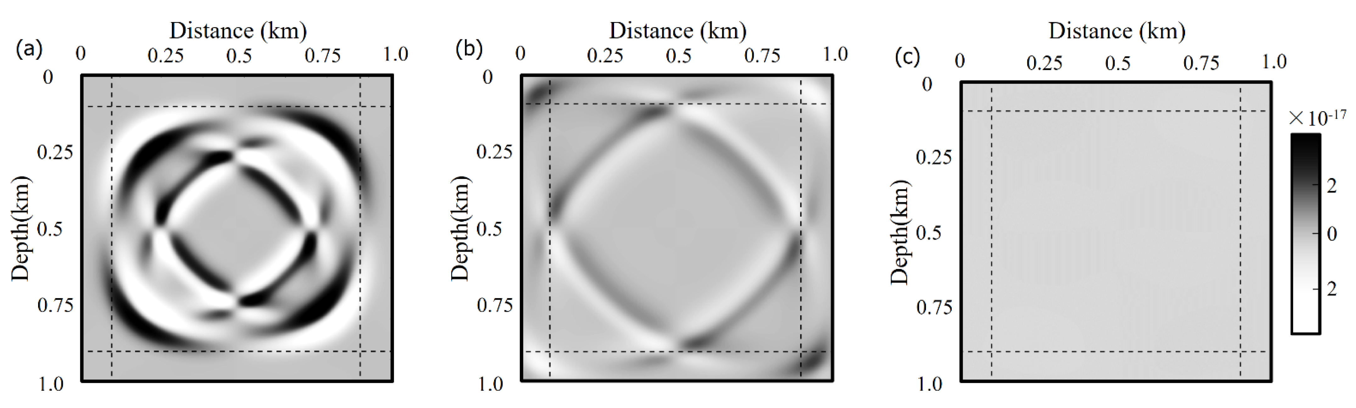
In the first test, the physical properties are given in Table 1: medium 1. We set the model size to be $1.0\mathrm{km}\times 1.0\mathrm{km}$ with a grid space of 2.5 m, and employed an explosive Ricker wavelet source with a dominant frequency of 20 Hz. Figure 5 exhibits snapshots of horizontal displacement and its corresponding analytical group velocity calculated from medium 1. These snapshots were simulated using PML and M-PML, respectively, at different times. Figure 5a,b are the snapshots computed inside the PML and M-PML at 0.1667 s. The consistency between the wavefront calculated from the analytical group velocity and the wavefront of snapshots can be observed in Figure 5c. Similar to the figures above, Figure 5d–f are recorded at 0.2444 s. The wavefront of snapshots is almost the same as the wavefront calculated from the analytical group velocity, and the absorptive capacity of M-PML is superior to that of PML at four corners. Figure 5g,h are recorded at 0.7 s, and the absorptive advantage of M-PML over PML can be observed. Figure 5i shows the wavefield energy decay curves in the computational domain. These results show that the absorption performance of M-PML is better than that of PML when both ABCs remain stable, which can be verified by the comparative observations in Figure 5g,h. Because at 0.7 s, the effective wavefield has all propagated within the boundary, while the boundary reflections observed in PML are stronger at this time, and that of M-PML is much weaker. To further quantitatively compare the performance of the two ABCs, we gave the energy curves of them, where the horizontal axis is time, and the vertical axis is the logarithm of energy, and we can see that the energy of the waves of both ABCs becomes weaker as time passes, but the energy of M-PML decays faster than that of PML. In addition, in order to verify the absorptive capacity and reliability of M-PML in viscous media, the wavefield snapshots of M-PML in viscoelastic anisotropic media are given in Figure 6. From these results, we know that M-PML is still effective in viscous anisotropic media.

Regarding the verification of the results, we calculated the wavefront using the analytical group velocity in anisotropic media [31], and the results are displayed in Figure 5c,f, where the fast propagating wavefront is the P-wave, and the slow one is the S-wave. It can be seen that the wavefield snapshots at the corresponding moment also contain P-waves and S-waves. The wavefront in snapshots can correspond well with the analytical wavefront in Figure 5c,f, which illustrates the reasonableness and applicability of the numerical results.

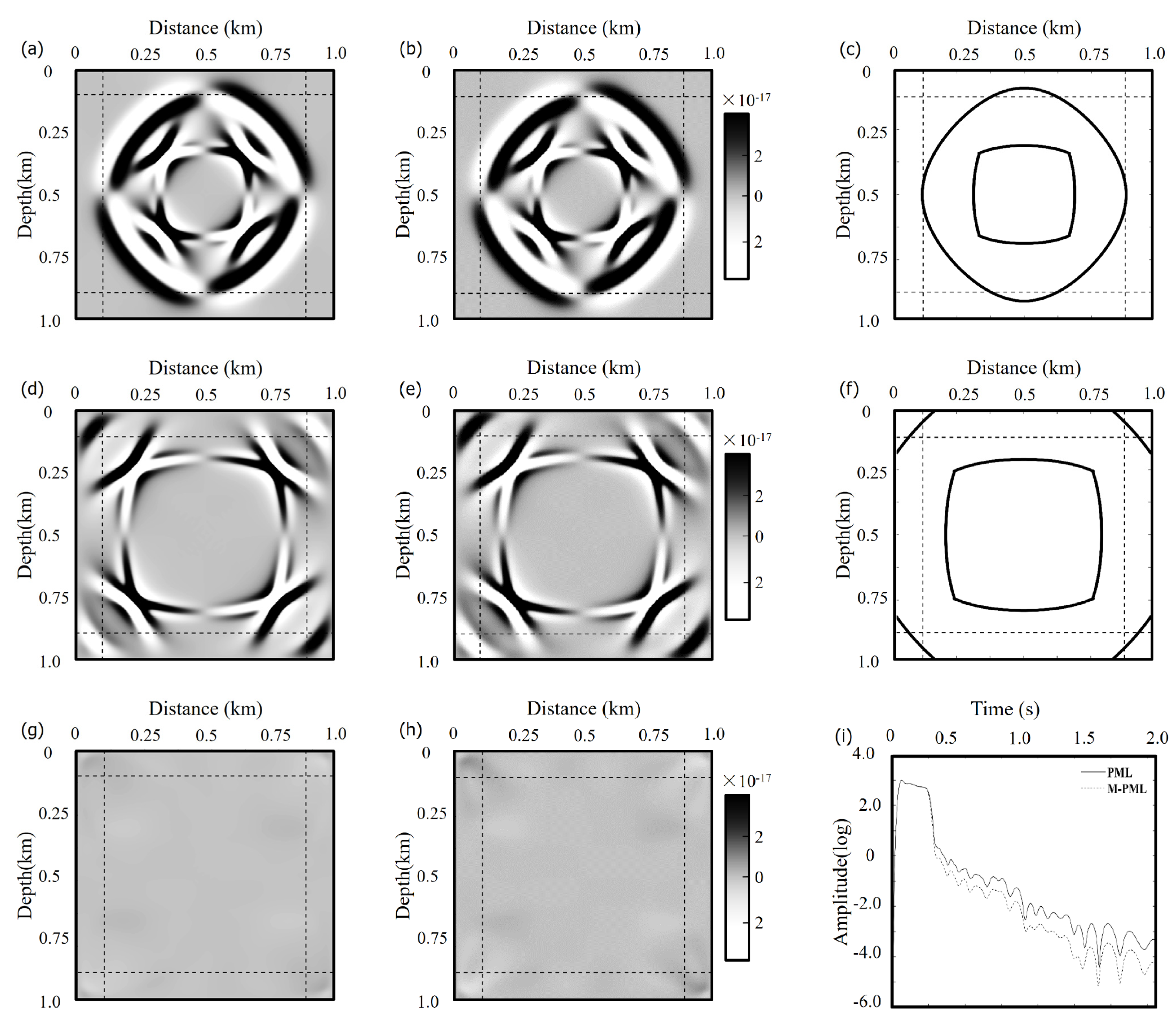
We further tested our algorithm with medium 2 in this test. The physical properties are given in Table 1. We also set the model size to be $1.0\mathrm{km}\times 1.0\mathrm{km}$ with a grid space of 2.5 m and employed an explosive Ricker wavelet source with a dominant frequency of 20 Hz. Figure 7 shows snapshots of horizontal displacement and its analytical wavefront calculated from medium 2. These snapshots are calculated within the PML and M-PML boundary conditions, respectively. Figure 7a,b are the snapshots simulated inside the PML and M-PML at 0.1222 s, respectively; Figure 7d,e are simulated inside the PML and M-PML at 0.1889 s, respectively; and the wavefront calculated by the analytical group velocity in Figure 7c,f are consistent with the wavefront of snapshots at 0.1222 s and 0.1889 s, respectively. Figure 7g,h are recorded at 0.6 s, and significant reflections can be observed at the four corners in the snapshot of the PML; however, the M-PML does not. Figure 7i shows the energy decay curves of the wavefield calculated from medium 2. This numerical experiment was conducted to confirm that M-PML has superior absorption performance to PML in arbitrarily different anisotropic media. It can still be seen from the results that the wavefront in the wavefield snapshots Figure 7a,b coincides with the analytical wavefront [31] Figure 7c,f at the corresponding moment, verifying the rationality and applicability of the numerical results. Similar to the previous section, viscosity is still introduced in this medium, and its wavefield snapshots are displayed in Figure 8 to confirm that M-PML can still maintain good absorptive properties and stability in different viscous anisotropic media.

Regarding absorption performance, observing the wavefield snapshots of PML and M-PML shows that both ABCs are stable in this homogenous anisotropic medium, so it is possible to compare their absorption performance visually. At 0.6 s, the effective wavefield wholly left the working area, and we can see that the boundary reflections of PML are strong at the four corners in Figure 7h, but those of M-PML are well attenuated. Further, in Figure 7i, it is illustrated that the energy decay curve of M-PML is lower than that of PML, which quantitatively displays the absorption advantage of M-PML over PML.

3.3. Wave Propagation in a Complex Anisotropic Medium

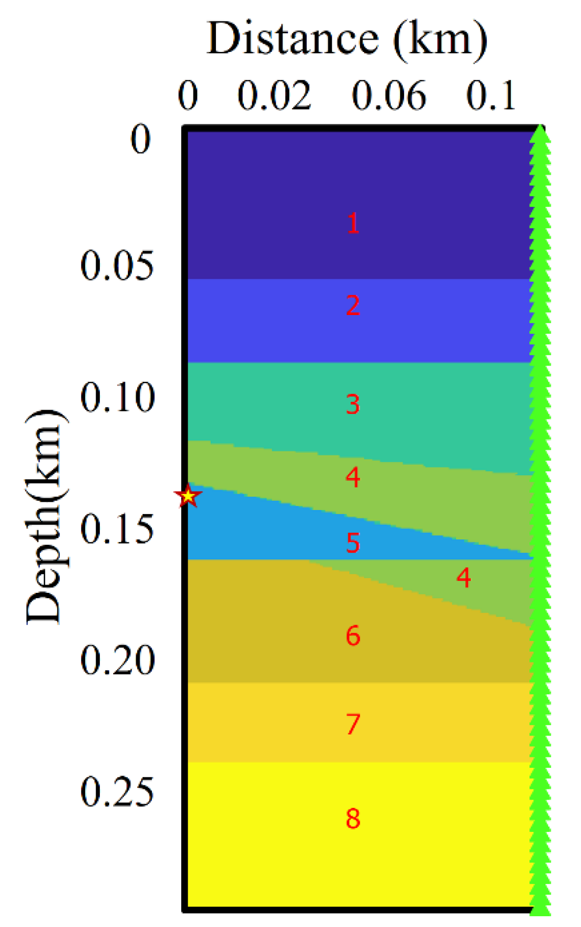
Finally, we used the frequency domain method based on M-PML to perform wavefield simulation for a more complicated cross-well model. The cross-well model is shown in Figure 9. The corresponding parameters selected are as follows: computing area, $0\le x\le 108\mathrm{m}$, $0\le z\le 289\mathrm{m}$; spatial step, $h=\mathrm{\Delta }x=\mathrm{\Delta }z=0.5\mathrm{m}$; grid parameter, $578\times 216$; the number of M-PML layers, 30; dominant frequency of the source, 130 Hz, the location of the source: $\left(135\mathrm{m},0\mathrm{m}\right)$; receiver alignment positions: $x=108\mathrm{m}$, $0.5\le z\le 288.5\mathrm{m}$; receiver interval, $2\mathrm{m}$. The cross-well model has eight layers. There are numerical constants in red in Figure 8, which label the layers in the figure. The red constants 1–8 in the figure correspond to layers 1–8 in

Table 2. Physical parameters used for the cross-well model.

Layer Media	Vp (m/s)	Vs (m/s)	Qp	Qs	ε	δ	ρ (kg/m3)
Layer 1	1875	826	10	10	0.225	0.100	2000
Layer 2	2202	969	10	10	0.015	0.060	2250
Layer 3	2868	1350	15	15	0.970	−0.090	1860
Layer 4	3368	1829	21	18	0.110	−0.035	2500
Layer 5	3688	2774	30	19	0.081	0.057	2730
Layer 6	3901	2682	38	25	0.137	−0.012	2640
Layer 7	4296	2471	42	35	0.081	0.129	2660
Layer 8	4529	2703	50	40	0.034	0.211	2520

, respectively. The asterisk in the figure represents the source. These anisotropic medium parameters are taken from the true sedimentary and are available in the study of Thomsen [28].

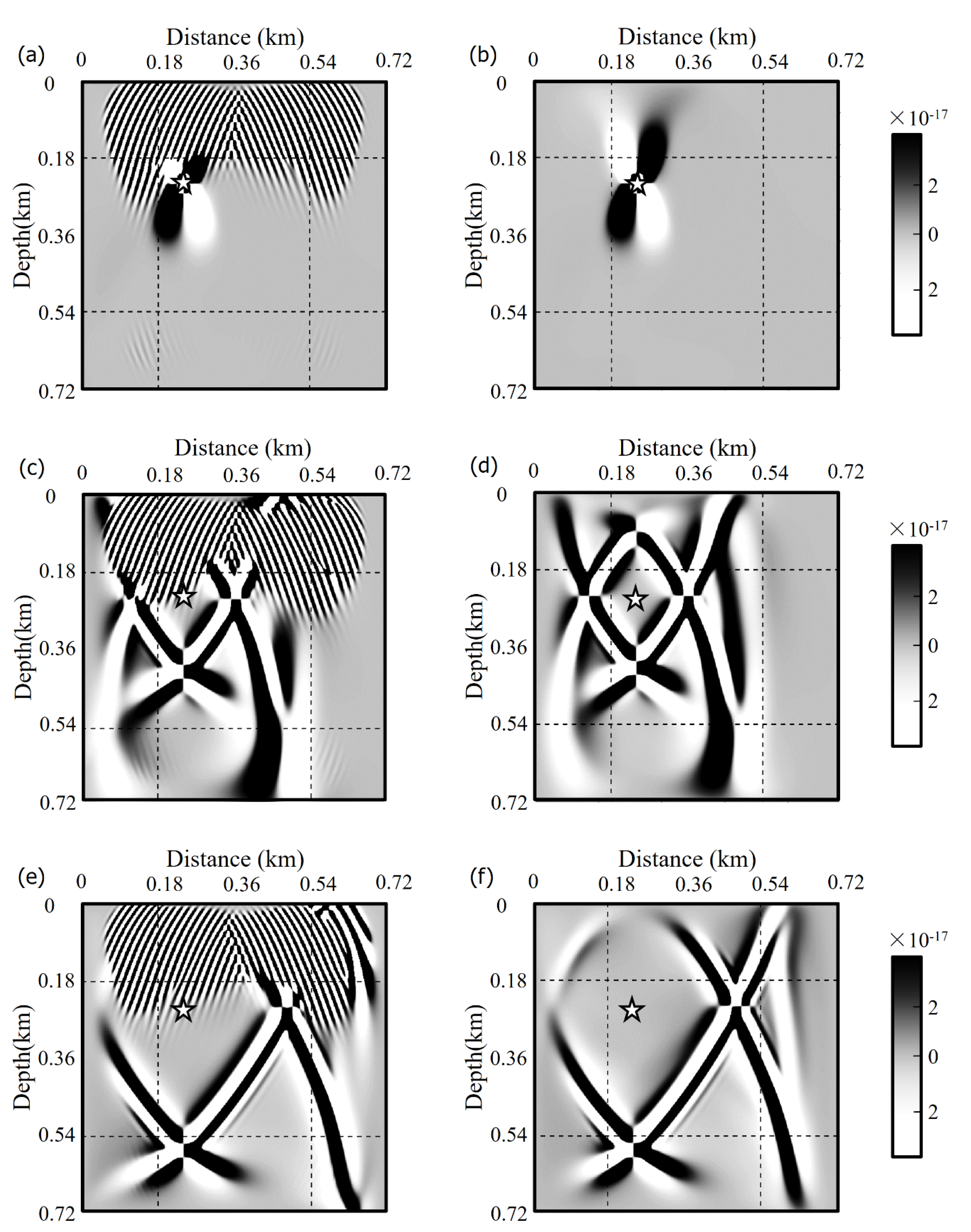
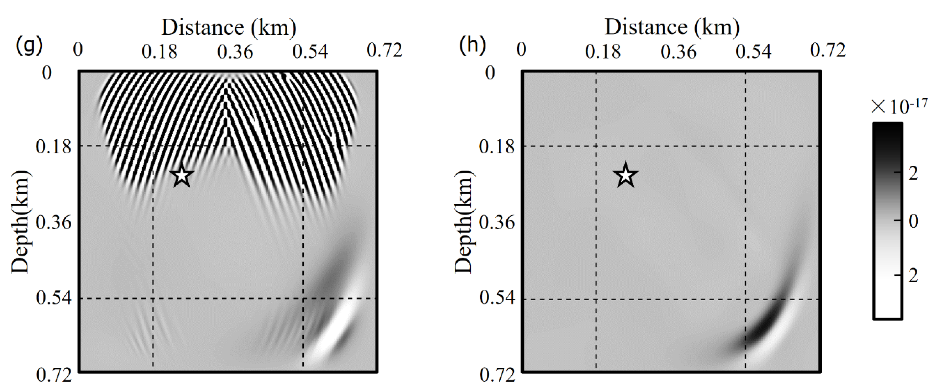
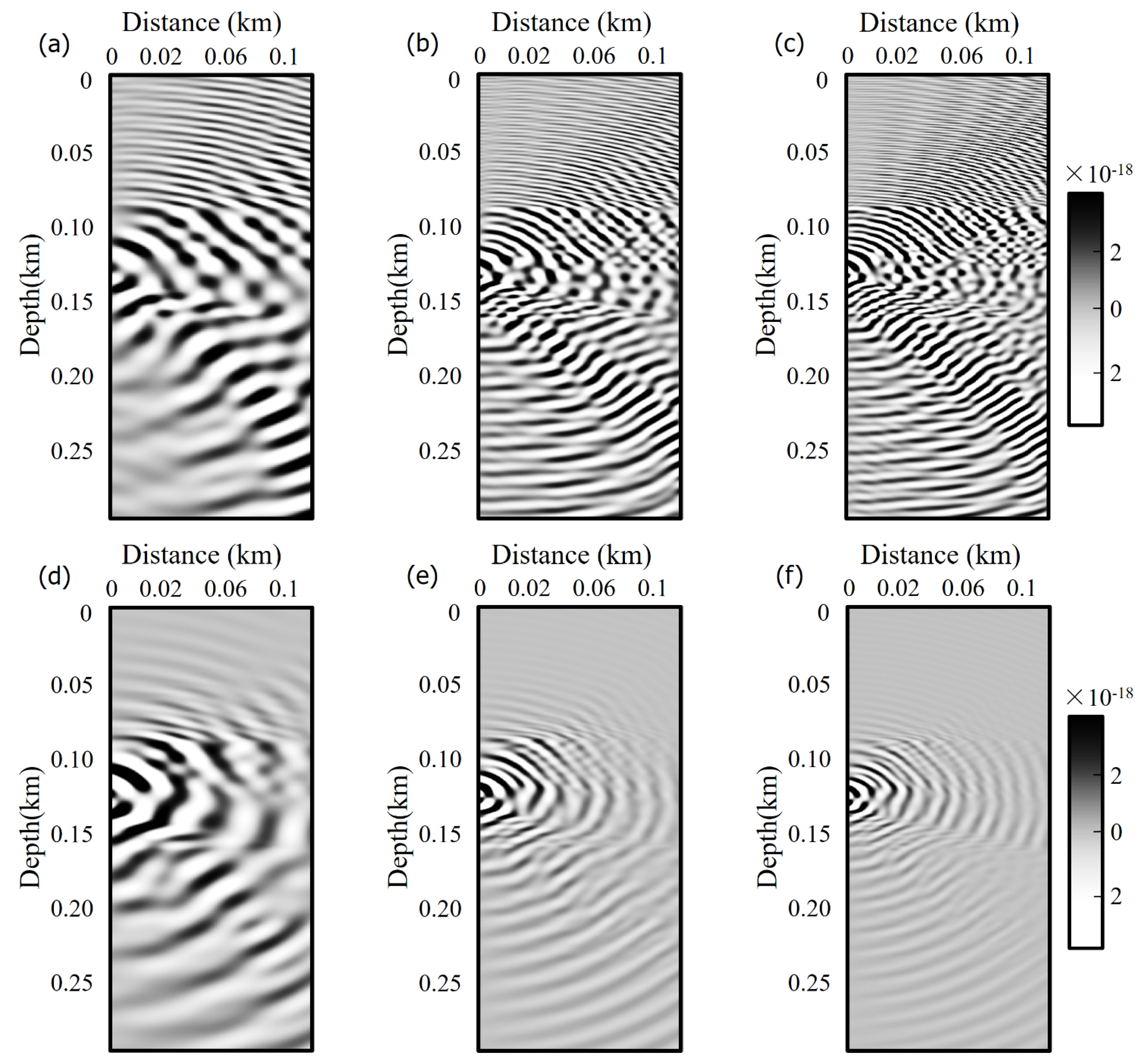
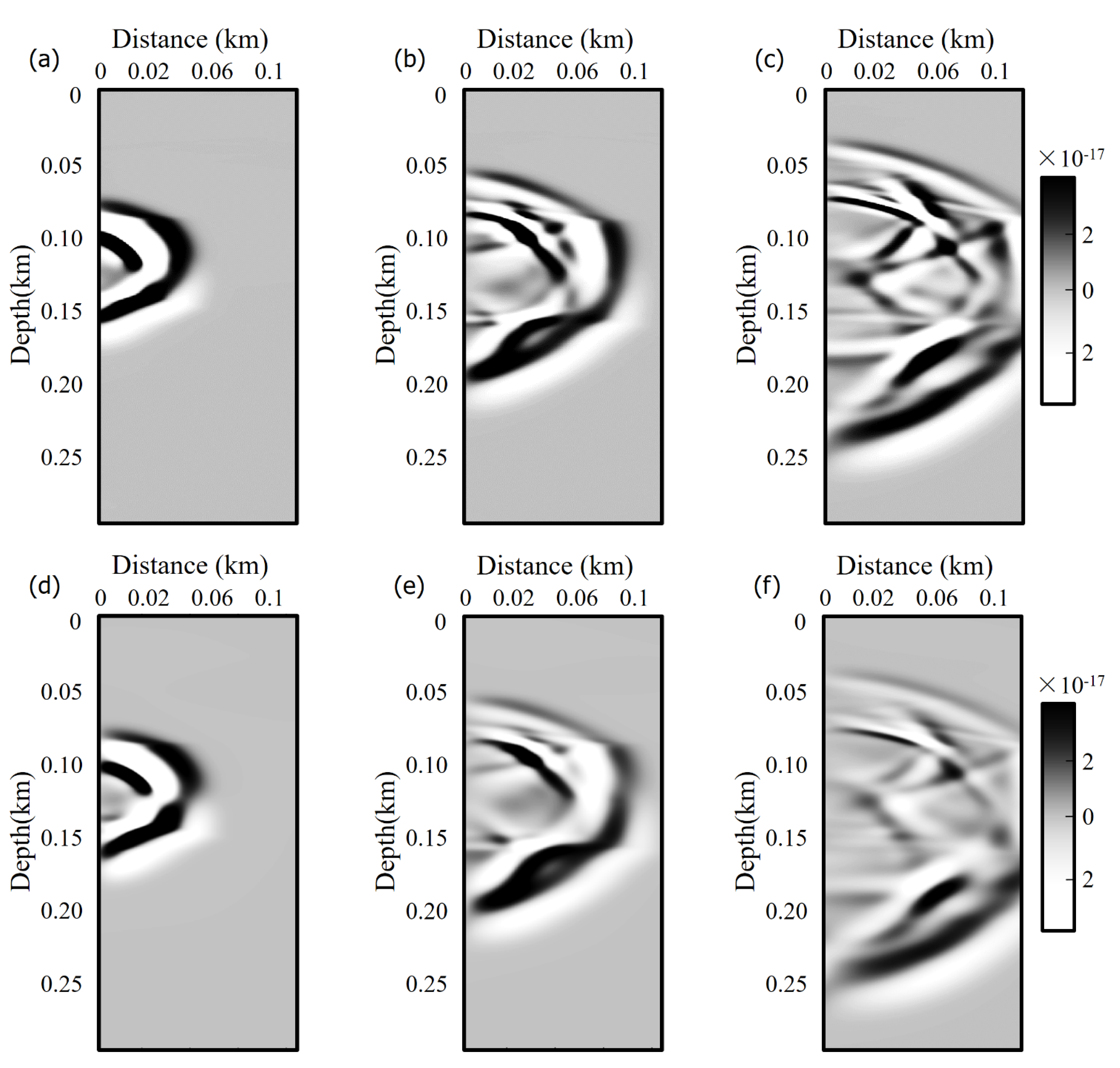
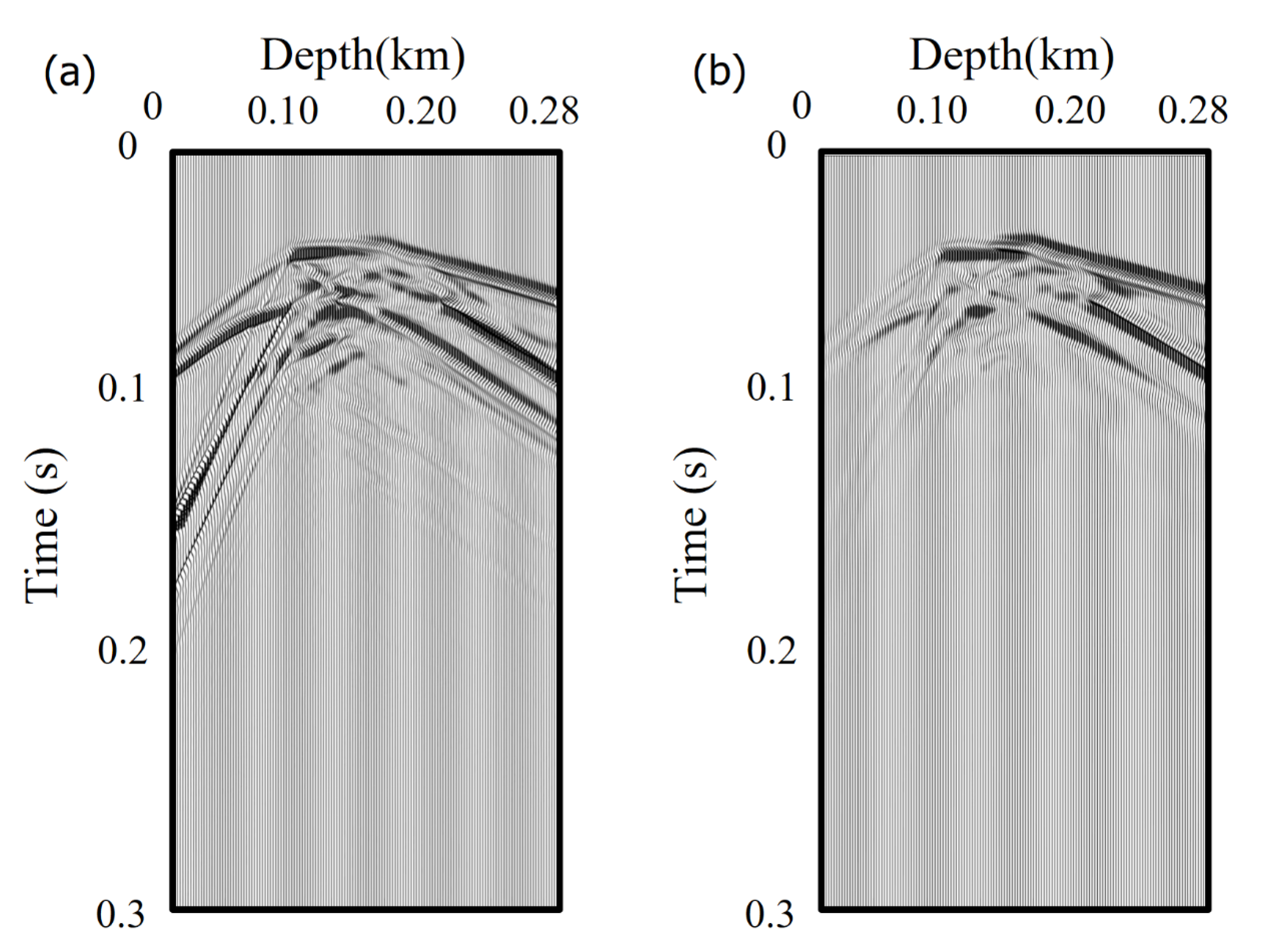
Figure 10 shows the mono-frequency wavefield snapshots of elastic and viscoelastic anisotropy obtained by the proposed method at 163.2 Hz, 329.8 Hz, and 429.5 Hz. Furthermore, the time-domain snapshots at the time point of 0.0199 s, 0.0299 s, and 0.0399 s computed by the proposed method are shown in Figure 11, respectively. It is easy to see that there exist no artificial edge effects near the truncated boundary in either the elastic or viscoelastic anisotropic wavefield. Then, we give the single-shot seismograms of the cross-well model, which are shown in Figure 12, and we also see that there exist no numerical dispersion or artificial edge effects in either elastic or viscoelastic anisotropic seismograms. Thus, we may conclude that the M-PML for the finite-difference frequency domain is suitable for wavefield simulation in a viscoelastic anisotropic and complicated medium.

4. Conclusions

In this study, in order to solve the instability of the absorbing boundary conditions caused by the frequency-domain algorithm for viscoelastic anisotropic wavefields, wave propagation was simulated by the finite-difference frequency-domain, and the reliability of the results was verified by combining the analytical wavefront obtained from the anisotropic analytical group velocity. The multi-axis perfectly matched layer (M-PML) was introduced in the frequency domain. We compared the wavefield snapshots and energy attenuation curves of M-PML and PML in different elastic anisotropic media. Then, we gave the viscoelastic anisotropic wavefield to demonstrate the reliability of M-PML in viscous media. The results indicate that M-PML can still stably and effectively absorb reflections from the truncated boundaries in strongly anisotropic and viscous media. Simulations in a complex cross-well viscoelastic anisotropic model indicate the applicability of this algorithm to a heterogeneous medium.

Moreover, the implementation of M-PML only needs to combine the damping profiles of PML, which improves absorption performance and stability while maintaining computational efficiency. In practice, this algorithm can be used as a forward operator for seismic migration, waveform inversion, and wave equation travel-time tomography. The frequency-domain algorithm can also improve the inversion efficiency of multi-source problems. For complex subsurface media, the proposed method can be applied for inversion of medium anisotropy and attenuation properties. Although our proposed algorithm works well, it has some limitations. Bad choices of $p^{\left(z/x\right)}$ and $p^{\left(x/z\right)}$ may lead to artificial reflections.

References

- Hestholm, S. Acoustic VTI modeling using high-order finite differences. Geophysics 2009, 74, T67. [Google Scholar] [CrossRef]
- Zhu, H.; Zhang, W.; Chen, X. Two-dimensional seismic wave simulation in anisotropic media by non-staggered finite difference method. Chin. J. Geophys. 2009, 52, 1536–1546. [Google Scholar]
- Qiao, Z.; Sun, C.; Wu, D. Theory and modeling of constant-Q viscoelastic anisotropic media using fractional derivative. Geophys. J. Int. 2019, 217, 798–815. [Google Scholar] [CrossRef]
- Devaney, A.J. Geophysical Diffraction Tomography. IEEE Trans. Geosci. Remote Sens. 1984, GE-22, 3–13. [Google Scholar] [CrossRef]
- Pratt, R.G.; Worthington, M.H. The application of diffraction tomography to cross-hole seismic data. Geophysics 1988, 53, 1284–1294. [Google Scholar] [CrossRef] [Green Version]
- Baysal, E.; Kosloff, D.; Sherwood, J. Reverse time migration. Geophysics 1983, 48, 1514–1524. [Google Scholar] [CrossRef] [Green Version]
- McMechan, G. Migration by extrapolation of time-dependent boundary values. Geophys. Prospect. 1983, 31, 413–420. [Google Scholar] [CrossRef]
- Dai, W.; Wang, X.; Schuster, G. Least-squares migration of multi-source data with a deblurring filter. Geophysics 2011, 76, R135–R146. [Google Scholar] [CrossRef]
- Tarantola, A. Inversion of seismic reflection data in the acoustic approximation. Geophysics 1984, 49, 1259–1266. [Google Scholar] [CrossRef]
- Pratt, R.G.; Worthington, M.H. Acoustic wave equation inverse theory applied to multi-source cross-hole tomography Part I: Acoustic wave-equation method. Geophys. Prospect. 1990, 38, 287–310. [Google Scholar] [CrossRef]
- Virieux, J.; Operto, S. An overview of full-waveform inversion in exploration geophysics. Geophysics 2009, 74, WCC1–WCC26. [Google Scholar] [CrossRef]
- Marfurt, K.J. Accuracy of finite difference and finite element modeling of scalar and elastic wave equations. Geophysics 1984, 49, 533–549. [Google Scholar] [CrossRef]
- Ben-Hadj-Ali, H.; Operto, S.; Virieux, J. An efficient frequency-domain full-waveform inversion method using simultaneous encoded sources. Geophysics 2011, 76, 109–124. [Google Scholar] [CrossRef]
- Operto, S.; Virieux, J.; Ribodetti, A.; Anderson, J.E. Finite-difference frequency-domain modeling of viscoacoustic wave propagation in 2D tilted transversely isotropic (TTI) media. Geophysics 2009, 74, 75–95. [Google Scholar] [CrossRef] [Green Version]
- Jeong, W.; Min, D.J.; Lee, G.H.; Lee, H.Y. 2D frequency-domain elastic full waveform inversion using finite-element method for VTI media. In SEG Technical Program. Expanded Abstracts 2011; SEG: San Antonio, TX, USA, 2011; pp. 2654–2658. [Google Scholar]
- Zhou, B.; Won, M.; Greenhalgh, S.; Liu, X. Generalizeded stiffness reduction method to remove the artificial edge-effects for seismic wave modeling in elastic anisotropic media. Geophys. J. Int. 2020, 220, 1394–1408. [Google Scholar] [CrossRef]
- Yang, Q.; Zhou, B.; Riahi, M.; Ai-Khaleel, M. A new generalized stiffness reduction method for 2D/2.5D frequency domain seismic wave modeling in viscoelastic anisotropic media. Geophysics 2020, 85, T315–T329. [Google Scholar] [CrossRef]
- Berenger, J.P. A perfectly matched layer for the absorption of electromagnetic waves. J. Comput. Phys. 1994, 114, 185–200. [Google Scholar] [CrossRef]
- Francis, C.; Tsogka, C. Application of the perfectly matched absorbing layer model to the linear elastodynamic problem in anisotropic heterogeneous media. Geophysics 2001, 66, 294–307. [Google Scholar]
- Komatitsch, D.; Tromp, J. A perfectly matched layer absorbing boundary condition for the second-order seismic wave equation. Geophys. J. Int. 2003, 154, 146–153. [Google Scholar] [CrossRef] [Green Version]
- Fang, X.; Niu, F. An unsplit complex frequency-shifted perfectly matched layer for second-order acoustic wave equations. Sci. China Earth Sci. 2021, 64, 992–1004. [Google Scholar] [CrossRef]
- Zhang, W.; Shen, Y. Unsplit complex frequency-shifted PML implementation using auxiliary differential equations for seismic wave modeling. Geophysics 2010, 75, T141–T154. [Google Scholar] [CrossRef] [Green Version]
- Opertp, S.; Virieux, J.; Amestoy, P.; L’Excellent, J.; Giraud, L.; Ali, H. 3D finite-difference frequency-domain modeling of visco-acoustic wave propagation using a massively parallel direct solver: A feasibility study. Geophysics 2007, 72, 195–211. [Google Scholar] [CrossRef] [Green Version]
- Oskooi, A.; Johnson, S.G. Distinguishing correct from incorrect PML proposals and a corrected unsplit PML for anisotropic dispersive media. J. Comput. Phys. 2011, 230, 2369–2377. [Google Scholar] [CrossRef]
- Meza-Fajardo, K.C.; Papageorgiou, A.S. A non-convolutional, split-field, perfectly matched layer for wave propagation in isotropic and anisotropic elastic media: Stability analysis. Bull. Seism. Soc. Am. 2008, 98, 1811–1836. [Google Scholar] [CrossRef]
- Ping, P.; Zhang, Y.; Xu, Y. A multi-axial perfectly matched layer (M-PML) for the long-time simulation of elastic wave propagation in the second-order equations. J. Appl. Geophys. 2014, 101, 124–135. [Google Scholar] [CrossRef]
- Zhang, Z.; Zhang, W.; Chen, X. Complex frequency-shifted multi-axial perfectly matched layer for elastic wave modeling on curvilinear grids. Geophys. J. Int. 2014, 198, 140–153. [Google Scholar] [CrossRef] [Green Version]
- Thomsen, L. Weak elastic anisotropy. Geophysics 1986, 51, 1954–1966. [Google Scholar] [CrossRef]
- Toksoz, M.N.; Johnston, D.H. Seismic Wave Attenuation; SEG Geophysical Reprint Series, No. 2; Society of Exploration Geophysicists: Houston, TX, USA, 1981. [Google Scholar]
- Zeng, Y.; He, J.; Liu, Q. The application of the perfectly matched layer in numerical modeling of wave propagation in poroelastic media. Geophysics 2001, 66, 1258–1266. [Google Scholar] [CrossRef]
- Daley, P.F.; Hron, F. Reflection and transmission coefficients for transversely isotropic media. Bull. Seism. Soc. Am. 1977, 67, 661–675. [Google Scholar] [CrossRef]
Figure 1.
Sketch map of the absorbing boundary condition (ABC). The square area in the middle is the computational area. The thick dashed-dot line represents the ABC applied outside the computational area.
Figure 2.
The second-order finite-difference star stencil used to model the viscoelastic anisotropic wave equation.
Figure 3.
Real part of the horizontal component from the monochromatic wavefield at 15 Hz with (a) classical PML and (b) M-PML.
Figure 4.
Snapshots of the horizontal component simulated with classical PML (a), (c), (e), (g) (left panel) and M-PML (b), (d), (f), (h) (right panel) at 0.0818 s, 0.2636 s, 0.4455 s, and 1.3046 s.
Figure 5.
Comparison between snapshots of the horizontal displacement in medium 1 at 0.1667 s, 0.2444 s, 0.7 s (a), (d), (g) calculated by M-PML and (b), (e), (h) PML. Wavefront calculated from analytical group velocity at (c) 0.1667 s and (f) 0.2444 s. (i) is the energy decay curve of PML and M-PML.
Figure 6.
Viscoelastic anisotropic wavefield of medium 1 calculated by M-PML at (a) 0.1667 s, (b) 0.2444 s, and (c) 0.7 s.
Figure 7.
Comparison between snapshots of the horizontal displacement in medium 2 at 0.1222 s, 0.1889 s, 0.6 s. (a), (d), (g) calculated by M-PML, and (b), (e), (h) PML. Wavefront calculated from analytical group velocity at (c) 0.1222 s and (f) 0.1889 s. (i) is the energy decay curve of PML and M-PML.
Figure 8.
Viscoelastic anisotropic wavefield of medium 2 calculated by M-PML at (a) 0.1222 s, (b) 0.1889 s, and (c) 0.6 s.
Figure 9.
Multi-layer cross-well model with single-excited source well on the left and multiple-received receiver well on the right, with red constants for medium numbers.
Figure 10.
Mono-frequency horizontal elastic anisotropic wavefield snapshots of different frequencies for the cross-well model at (a) 163.2 Hz, (b) 329.8 Hz, (c) 429.5 Hz, and viscoelastic anisotropic wavefield at (d) 163.2 Hz, (e) 329.8 Hz, and (f) 429.5 Hz.
Figure 11.
Time-domain horizontal elastic anisotropic wavefield snapshots for the cross-well model at (a) 0.02 s, (b) 0.03 s, (c) 0.04 s, and viscoelastic anisotropic wavefield at (d) 0.02 s, (e) 0.03 s, and (f) 0.04 s.
Figure 12.
Time-domain horizontal (a) elastic anisotropic and (b) viscoelastic anisotropic seismogram corresponding to Figure 11.