Design and Testing of a LUT Airfoil for Straight-Bladed Vertical Axis Wind Turbines

 , ,
, ,
Abstract
:1. Introduction
2. Basis and Method of Design for the LUT Airfoil
2.1. Design Basis
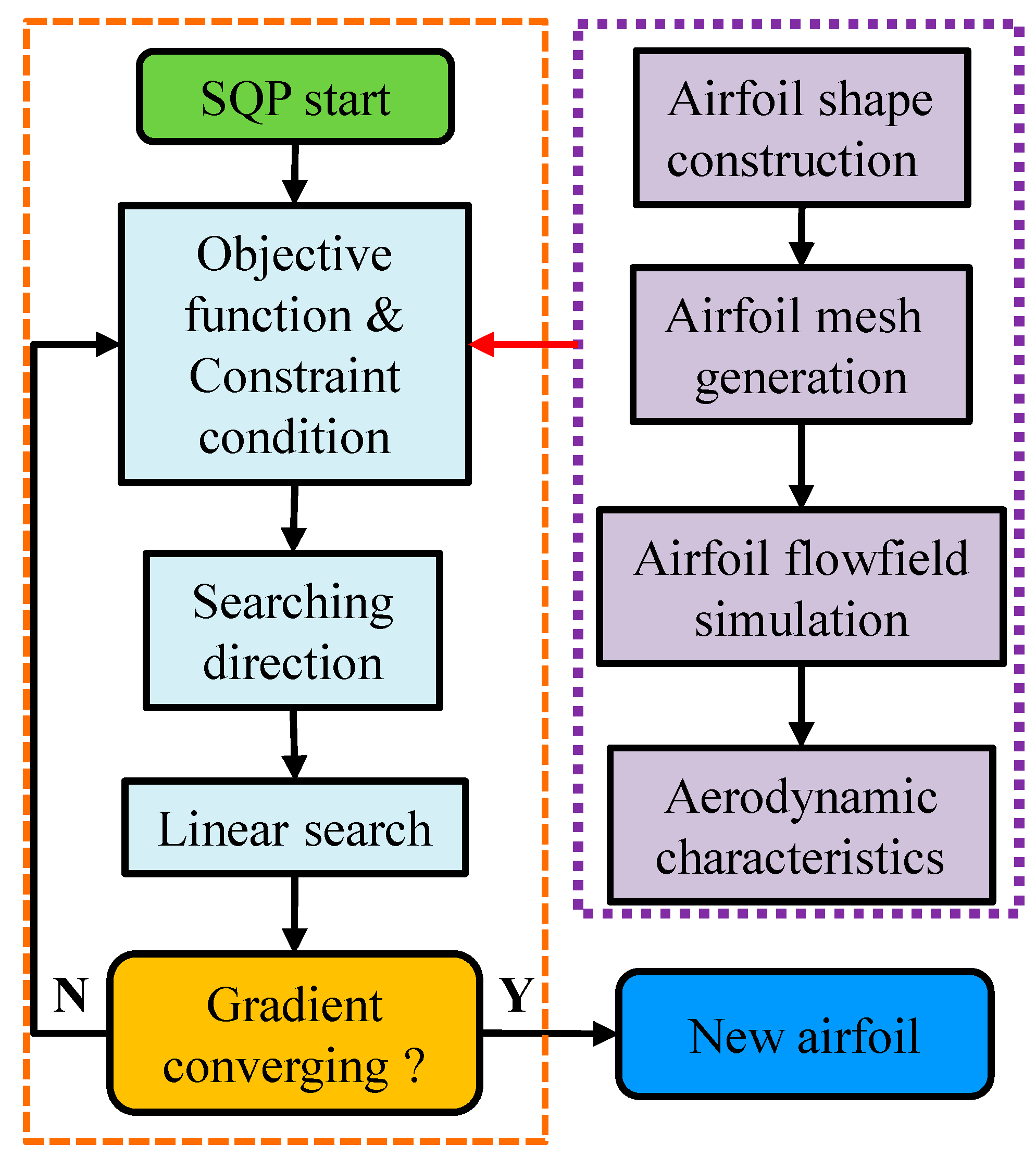
2.2. LUT Airfoil Optimization and Design Method
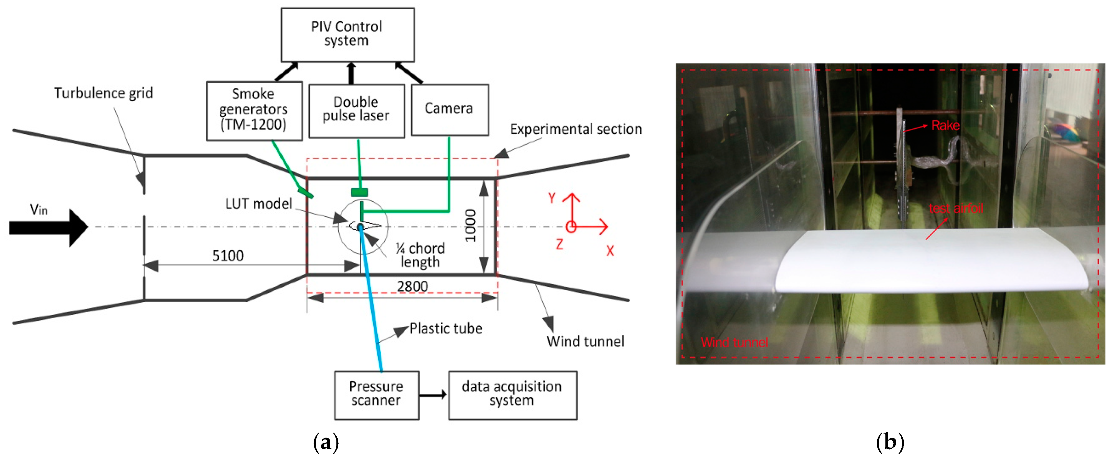
3. Experimental Equipment and Procedures
3.1. Wind Tunnel
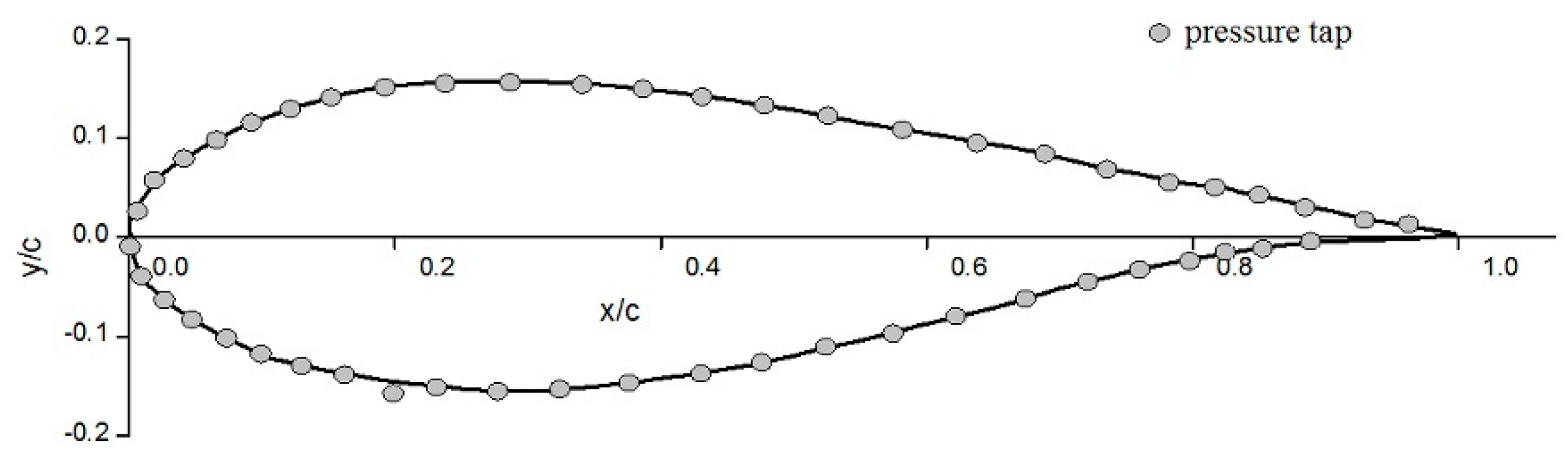
3.2. Test LUT Airfoil Model
3.3. Pressure Measurement and PIV (Particle Image Velocimetry) Devices
4. Results and Discussion
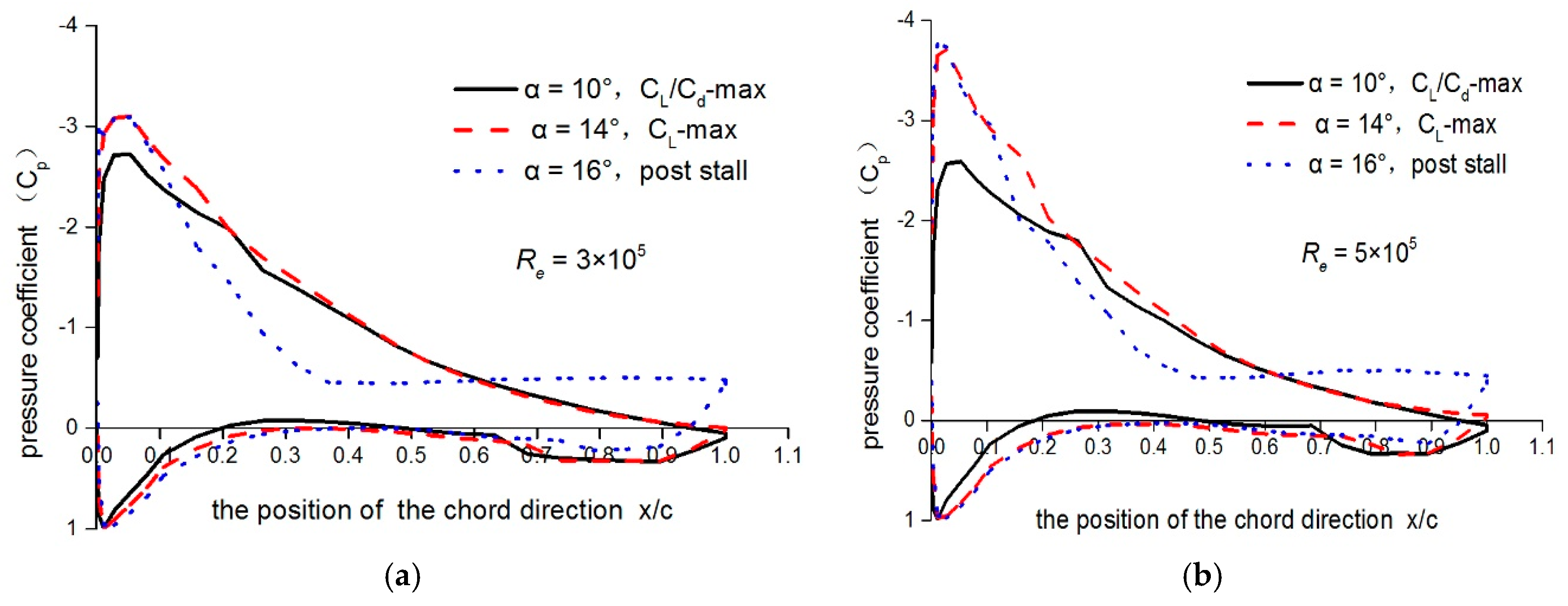
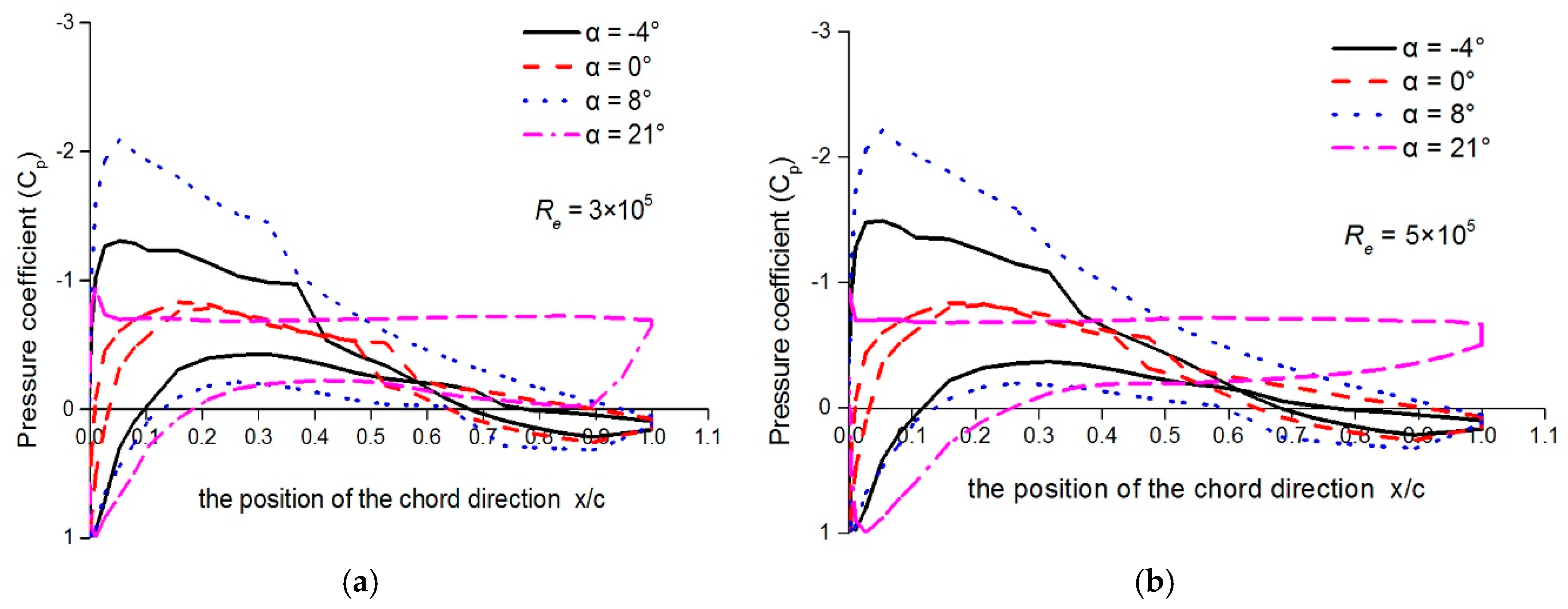
4.1. Static LUT Airfoil Performance at Low Reynolds Number
4.1.1. Pressure Coefficient Distribution on the Surface for the LUT Airfoil
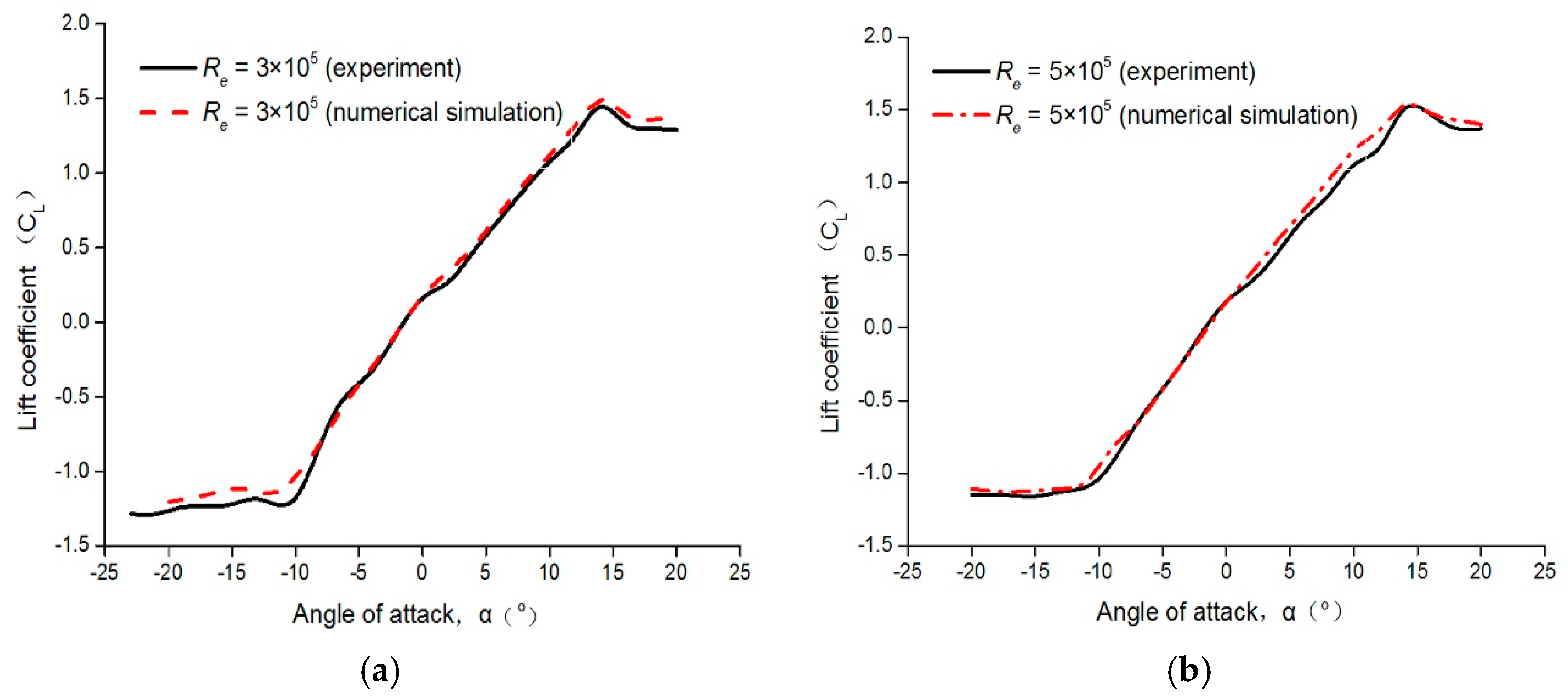
4.1.2. Lift Coefficient of the LUT Airfoil
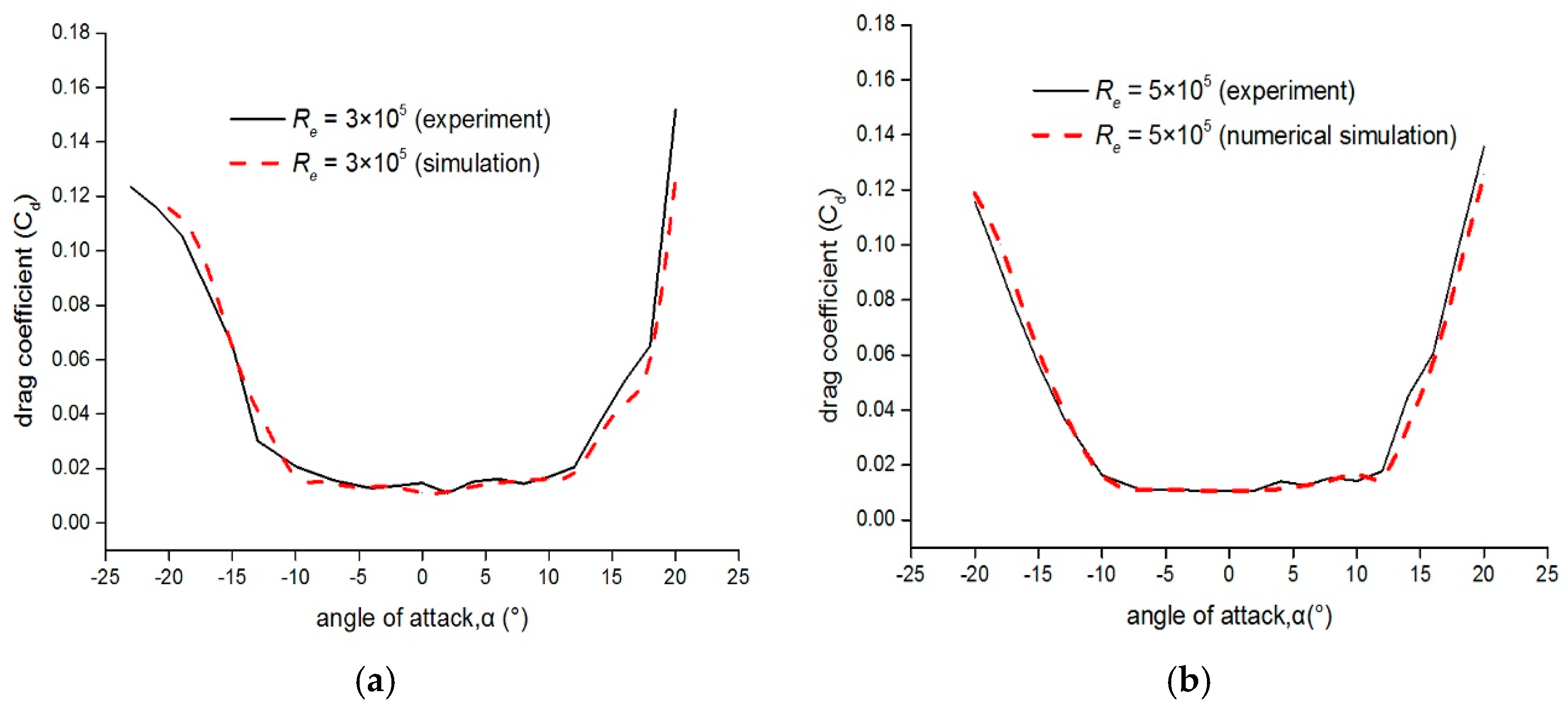
4.1.3. Drag Coefficient of the LUT Airfoil
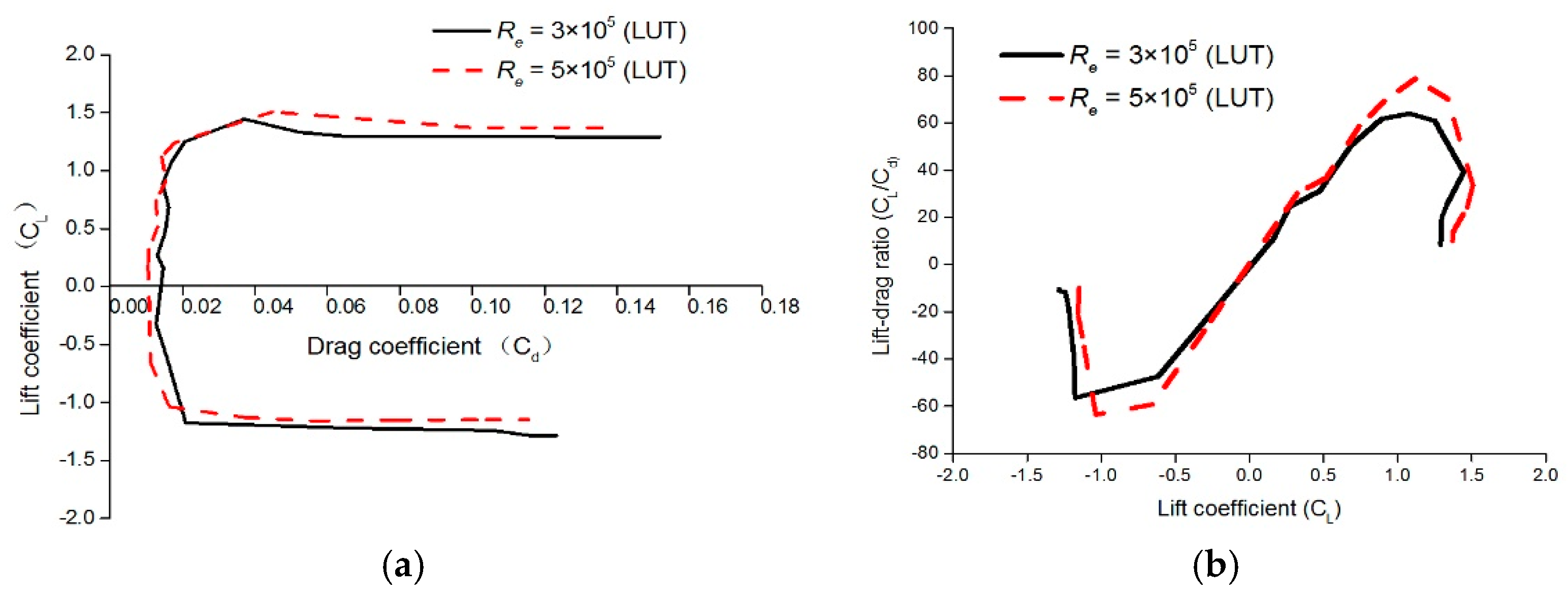
4.1.4. Lift–Drag Ratios of the LUT Airfoil
5. Conclusions
Author Contributions
Funding
Acknowledgments
Conflicts of Interest
Nomenclature
| H-VAWT | H-type Vertical Axis Wind Turbines |
| VAWT | Vertical Axis Wind Turbines |
| HAWT | Horizontal Axis Wind Turbines |
| LUT | The name of the newly designed airfoil (Lanzhou University of Technology) |
| DTU | Technical University of Denmark |
| SST | Shear Stress Transport |
| Re | Reynolds number |
| α | angle of attack, ° |
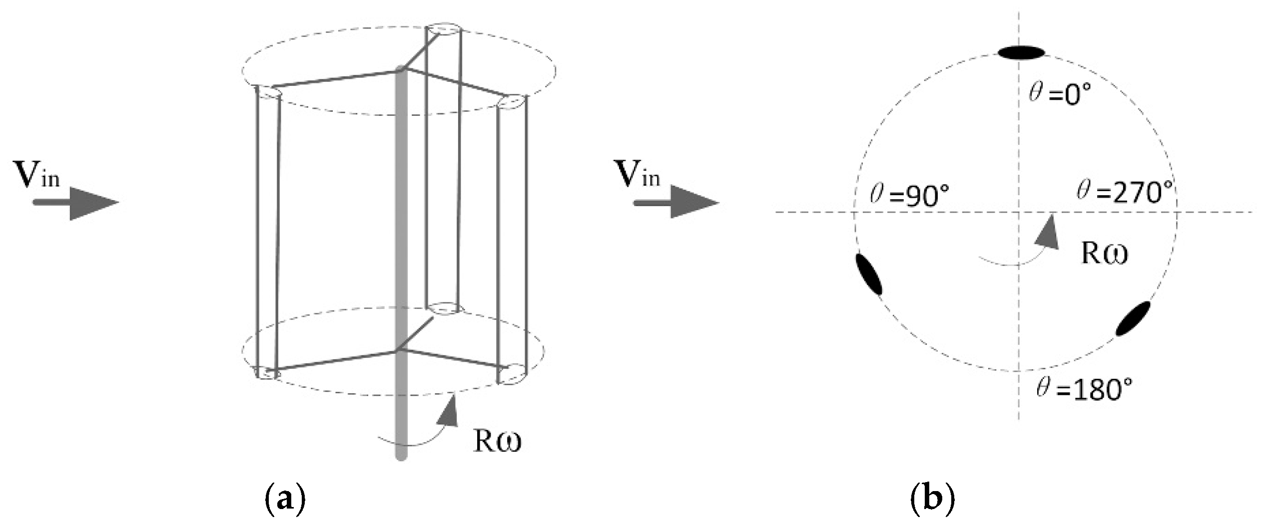
| θ | azimuthal angle, ° |
| ω | rotational speed of the wind turbine, rad/s |
| Vin | freestream velocity, m/s |
| R | rotor radius, m |
| C | airfoil chord length, mm |
| SQP | Sequential Quadratic Programming |
| σ | penalty factor |
| CL/Cd | lift–drag ratios |
| CL | lift coefficient |
| Cd | drag coefficient |
| r0 | leading-edge radius |
| Cp | Pressure coefficient |
| PIV | Particle Image Velocimetry |
| FS | Full Scale |
Appendix A

References
- Ho, A.; Mbistrova, A.; Corbetta, G. The European Offshore Wind Industry-Key Trends and Statistics 2015; Technical Report; European Wind Energy Association: Brussels, Belgium, February 2016. [Google Scholar]
- Battisti, L.; Benini, E.; Brighenti, A.; Dell’Anna, S.; Raciti Castelli, M. Small wind turbine effectiveness in the urban environment. Renew. Energy 2018, 129, 102–113. [Google Scholar] [CrossRef]
- Guo, Y.; Liu, L.; Gao, X.; Xu, W. Aerodynamics and Motion Performance of the H-Type Floating Vertical Axis Wind Turbine. Appl. Sci. 2018, 8, 262. [Google Scholar] [CrossRef]
- Kumar, R.; Raahemifar, K.; Fung, A.S. A critical review of vertical axis wind turbines for urban applications. Renew. Sustain. Energy Rev. 2018, 89, 281–291. [Google Scholar] [CrossRef]
- Li, Q.; Maeda, T.; Kamada, Y.; Ogasawara, T.; Nakai, A.; Kasuya, T. Investigation of power performance and wake on a straight-bladed vertical axis wind turbine with field experiments. Energy 2017, 141, 1113–1123. [Google Scholar] [CrossRef]
- Aslam Bhutta, M.M.; Hayat, N.; Farooq, A.U.; Ali, Z.; Jamil, S.R.; Hussain, Z. Vertical axis wind turbine—A review of various configurations and design techniques. Renew. Sustain. Energy Rev. 2012, 16, 1926–1939. [Google Scholar] [CrossRef]
- Sutherland, H.J.; Berg, D.E.; Ashwill, T.D. A Retrospective of VAWT Technology; Technical Report SAND2012-0304; Sandia National Laboratories: Albuquerque, NM, USA, January 2012.
- Kanyako, F.; Janajreh, I. Numerical Investigation of Four Commonly Used Airfoils for Vertical Axis Wind Turbine. In ICREGA’14-Renewable Energy: Generation and Application; Hamdan, M., Hejase, H., Noura, H., Fardoun, A., Eds.; Springer: Cham, Switzerland, 2014; pp. 443–454. [Google Scholar] [CrossRef]
- Islam, M. Analysis of Fixed-Pitch Straight-Bladed VAWT with Asymmetric Airfoils. Ph.D. Thesis, University of Windsor, Windsor, ON, Canada, 2008. [Google Scholar]
- Kirke, B.K. Evaluation of Self-Starting Vertical Axis Wind Turbines for Stand-Alone Appllications. Ph.D. Thesis, Griffith University, Brisbane, Australia, 1998. [Google Scholar]
- Rainbird, J.M.; Bianchini, A.; Balduzzi, F.; Peiró, J.; Graham, J.M.R.; Ferrara, G.; Ferrari, L. On the influence of virtual camber effect on airfoil polars for use in simulations of Darrieus wind turbines. Energy Convers. Manag. 2015, 106, 373–384. [Google Scholar] [CrossRef]
- Mohamed, M.H.; Ali, A.M.; Hafiz, A.A. CFD analysis for H-rotor Darrieus turbine as a low speed wind energy converter. Eng. Sci. Technol. Int. J. 2015, 18, 1–13. [Google Scholar] [CrossRef]
- Carrigan, T.J.; Dennis, B.H.; Han, Z.X.; Wang, B.P. Aerodynamic Shape Optimization of a Vertical-Axis Wind Turbine Using Differential Evolution. ISRN Renew. Energy 2012, 2012, 1–16. [Google Scholar] [CrossRef] [Green Version]
- Asr, M.T.; Nezhad, E.Z.; Mustapha, F.; Wiriadidjaja, S. Study on start-up characteristics of H-Darrieus vertical axis wind turbines comprising NACA 4-digit series blade airfoils. Energy 2016, 112, 528–537. [Google Scholar] [CrossRef]
- Chen, J.; Chen, L.; Xu, H.; Yang, H.; Ye, C.; Liu, D. Performance improvement of a vertical axis wind turbine by comprehensive assessment of an airfoil family. Energy 2016, 114, 318–331. [Google Scholar] [CrossRef]
- Sheldahl, R.E.; Klimas, P.C. Aerodynamic Characteristics of Seven Sysmmetrical Airfoil Sections Through 180-Degree Angle of Attack for Use in Aerodynamic Analysis of Vertical Axis Wind Turbines; Technical Report SAND80-2114; Sandia National Laboratories: Albuquerque, NM, USA, March 1981.
- Klimas, P.C. Tailored Airfoils for Vertical Axis Wind Turbines; Technical Report SAND84-1062; Sandia National Laboratories: Albuquerque, NM, USA, November 1984.
- Islam, M.; Fartaj, A.; Carriveau, R. Design analysis of a smaller-capacity straight-bladed VAWT with an asymmetric airfoil. Int. J. Sustain. Energy 2011, 30, 179–192. [Google Scholar] [CrossRef]
- Islam, M.; Ting, D.S.-K.; Fartaj, A. Desirable Airfoil Features for Smaller-Capacity Straight-Bladed VAWT. Wind Eng. 2007, 31, 165–196. [Google Scholar] [CrossRef]
- Ferreira, C.S.; Geurts, B. Aerofoil optimization for vertical-axis wind turbines. Wind Energy 2015, 18, 1371–1385. [Google Scholar] [CrossRef]
- Ragni, D.; Ferreira, C.S.; Correale, G. Experimental investigation of an optimized airfoil for vertical-axis wind turbines. Wind Energy 2015, 18, 1629–1643. [Google Scholar] [CrossRef]
- Batista, N.C.; Melício, R.; Mendes, V.M.F.; Calderón, M.; Ramiro, A. On a self-start Darrieus wind turbine: Blade design and field tests. Renew. Sustain. Energy Rev. 2015, 52, 508–522. [Google Scholar] [CrossRef]
- Bedon, G.; Betta, S.D.; Benini, E. Performance-optimized airfoil for Darrieus wind turbines. Renew. Energy 2016, 94, 328–340. [Google Scholar] [CrossRef]
- Hand, B.; Kelly, G.; Cashman, A. Numerical simulation of a vertical axis wind turbine airfoil experiencing dynamic stall at high Reynolds numbers. Comput. Fluids 2017, 149, 12–30. [Google Scholar] [CrossRef]
- Sargent, R.W.H.; Ding, M. A New SQP Algorithm for Large-Scale Nonlinear Programming. SIAM J. Optim. 2001, 11, 716–747. [Google Scholar] [CrossRef]
- Andrei, N. Sequential Quadratic Programming Continuous (SQP). In Nonlinear Optimization for Engineering Applications in GAMS Technology, 1st ed.; Springer: Cham, Switzerland, 2017; Volume 121, pp. 269–288. ISBN 978-3-319-58355-6. [Google Scholar]
- Howell, R.; Qin, N.; Edwards, J.; Durrani, N. Wind tunnel and numerical study of a small vertical axis wind turbine. Renew. Energy 2010, 35, 412–422. [Google Scholar] [CrossRef] [Green Version]
- Airfoil Tools. Available online: http://airfoiltools.com/ (accessed on 1 September 2018).
- Timmer, W.A.; Van Rooij, R.P.J.O.M. Summary of the Delft University Wind Turbine Dedicated Airfoils. J. Sol. Energy Eng. 2003, 125, 488–496. [Google Scholar] [CrossRef]
- Fuglsang, P.; Bak, C. Development of the Risø wind turbine airfoils. Wind Energy 2004, 7, 145–162. [Google Scholar] [CrossRef]
- Meng, X.; Hu, H.; Yan, X.; Liu, F.; Luo, S. Lift improvements using duty-cycled plasma actuation at low Reynolds numbers. Aerosp. Sci. Technol. 2018, 72, 123–133. [Google Scholar] [CrossRef]
- Anderson, J.D. Fundamentals of Aerodynamics, 5th ed.; McGraw-Hill Education: New York, NY, USA, 2011; ISBN 9780073398105. [Google Scholar]
- Somers, D.M. Design and Experimental Results for the S825 Airfoil Period of Performance: 1998–1999 Design and Experimental Results for the S825 Airfoil; Technical Report NREL/SR-500-36346; National Renewable Energy Laboratory: Golden, CO, USA, 2005.
- Balduzzi, F.; Bianchini, A.; Maleci, R.; Ferrara, G.; Ferrari, L. Critical issues in the CFD simulation of Darrieus wind turbines. Renew. Energy 2016, 85, 419–435. [Google Scholar] [CrossRef]
- Zhang, X.; Wang, G.; Zhang, M.; Liu, H.; Li, W. Numerical study of the aerodynamic performance of blunt trailing-edge airfoil considering the sensitive roughness height. Int. J. Hydrogen Energy 2017, 42, 18252–18262. [Google Scholar] [CrossRef]


| Airfoil | Re (1 × 10⁵) | Max. Thickness | (x/c) Max. Thickness | Max. Camber | (x/c) Max. Camber | Radius Leading Edge (r0/c) | Max. CL/Cd (α) | Max. CL (α) |
|---|---|---|---|---|---|---|---|---|
| Du06-W-200 [28] | 3 | 19.8% | 31.1% | 0.5% | 84.6% | 1.7442% | 58.05 (9.75°) | 1.4153 (16.75°) |
| 5 | 71.5 (9.5°) | 1.4384 (18°) | ||||||
| NACA0018 [28] | 3 | 18% | 30% | 0 | 0 | 3.1017% | 57.09 (8.25°) | 1.24 (18.75) |
| 5 | 65.8 (9.25°) | 1.2624 (16.5°) | ||||||
| NACA0015 [28] | 5 | 15% | 30% | 0 | 0 | 2.3742% | 66.43 (7.5°) | 1.2731 (16.75°) |
| DU12W262 [21] | - | 26.2% | 37% | - | - | - | - | - |
| AIR013 [20] | - | 34.9% | - | 2.29% | - | 7.8% | - | - |
© 2018 by the authors. Licensee MDPI, Basel, Switzerland. This article is an open access article distributed under the terms and conditions of the Creative Commons Attribution (CC BY) license (http://creativecommons.org/licenses/by/4.0/).
Share and Cite
Li, S.; Li, Y.; Yang, C.; Zhang, X.; Wang, Q.; Li, D.; Zhong, W.; Wang, T. Design and Testing of a LUT Airfoil for Straight-Bladed Vertical Axis Wind Turbines. Appl. Sci. 2018, 8, 2266. https://0-doi-org.brum.beds.ac.uk/10.3390/app8112266
Li S, Li Y, Yang C, Zhang X, Wang Q, Li D, Zhong W, Wang T. Design and Testing of a LUT Airfoil for Straight-Bladed Vertical Axis Wind Turbines. Applied Sciences. 2018; 8(11):2266. https://0-doi-org.brum.beds.ac.uk/10.3390/app8112266
Chicago/Turabian StyleLi, Shoutu, Ye Li, Congxin Yang, Xuyao Zhang, Qing Wang, Deshun Li, Wei Zhong, and Tongguang Wang. 2018. "Design and Testing of a LUT Airfoil for Straight-Bladed Vertical Axis Wind Turbines" Applied Sciences 8, no. 11: 2266. https://0-doi-org.brum.beds.ac.uk/10.3390/app8112266