An Optimization Framework for Wind Farm Design in Complex Terrain

Featured Application

Analysis and optimization of wind farm design in complex terrain.

Abstract

Designing wind farms in complex terrain is an important task, especially for countries with a large portion of complex terrain territory. To tackle this task, an optimization framework is developed in this study, which combines the solution from a wind resource assessment tool, an engineering wake model adapted for complex terrain, and an advanced wind farm layout optimization algorithm. Various realistic constraints are modelled and considered, such as the inclusive and exclusive boundaries, minimal distances between turbines, and specific requirements on wind resource and terrain conditions. The default objective function in this framework is the total net annual energy production (AEP) of the wind farm, and the Random Search algorithm is employed to solve the optimization problem. A new algorithm called Heuristic Fill is also developed in this study to find good initial layouts for optimizing wind farms in complex terrain. The ability of the framework is demonstrated in a case study based on a real wind farm with 25 turbines in complex terrain. Results show that the framework can find a better design, with 2.70% higher net AEP than the original design, while keeping the occupied area and minimal distance between turbines at the same level. Comparison with two popular algorithms (Particle Swarm Optimization and Genetic Algorithm) also shows the superiority of the Random Search algorithm.

1. Introduction

In the past two decades, the world has witnessed a remarkable growth of wind energy development. According to the latest statistics from the Global Wind Energy Council (GWEC), the global cumulative installed wind capacity has increased from 23.9 GW in 2001 to 439.1 GW in 2017, representing an average annual increase by 20.4% [1]. Although offshore wind is now attracting a lot of interests and has grown rapidly in recent years, especially in northern Europe, today it represents only 4.3% of the global installed capacity of wind energy [2]. The dominance of onshore wind is mainly due to its longer development history, lower cost, and easier deployment.

As a result of the rapid growth of onshore wind, a lot of onshore wind farms have been built worldwide. Since many suitable sites in flat terrain have already been developed with wind farms, more and more wind farms are going to be built in complex terrain, especially for countries featured by a large percentage of topography covered with mountains, such as China.

Compared with a wind farm on flat terrain, a wind farm built on complex terrain benefits from the possible richer wind resource at certain locations (brought by the speed-up effect due to the terrain topography change), but it is also more likely to be exposed to more complex flow conditions, higher fatigue loads, more expensive installation, operation and maintenance costs, and other disadvantages [3].

Designing wind farms in complex terrain is not a trivial task, mainly due to the complex interactions of the boundary layer flow with the complex terrain and wind turbine wakes, and also due to the multi-disciplinary nature of the wind farm design problem. This problem typically involves different design and engineering tasks, which may come from technical, logistical, environmental, economical, legal, and/or even social considerations.

For most industrial practitioners, the design of wind farms conventionally concerns mainly the micro-siting of wind turbines based on consideration of wind resource, i.e., determining the exact position for each turbine at a selected wind farm site [4]. Typically, a wind farm developer/designer uses a wind resource assessment tool, such as WAsP [5] (the industry-standard PC software for wind resource assessment, siting, and energy yield calculations for wind turbines and wind farms), to assess the wind resource of the wind farm site based on wind measurement data during a period [6]. Then, the final design of the wind farm, mainly the layout of turbines, is determined for maximizing the annual energy production (AEP) while considering certain constraints, such as the proximity of wind turbines. This final layout is usually obtained by either manual adjustments or using some optimization techniques [7]. After finding the turbine layout, other design tasks related to foundations, access roads, electrical system, and other components or systems are handled separately, often by specialized engineering consulting companies.

The general problem of modelling the wind flow over complex terrain has been an important research field for a very long time. Seventy years ago, Queney published a review of theoretical models of inviscid flow over hills and mountains [8]. More recently, Wood gave a historical review of studies (until 2000) on wind flow over complex terrain [9]. Similarly, in the wind energy community, the problem of wind resource assessment in complex terrain was investigated by many researchers over a long period [10].

In contrast, wind farm design optimization has only become a hot research area quite recently and the majority of the published studies in this field deal with wind farms in flat terrain or offshore [11]. Few studies investigated the wind farm design optimization problems in complex terrain. Song et al. [12] proposed a bionic method for optimizing the turbine layout in complex terrain. In this study the objective was to maximize the power output, and the wake flow was simulated by using the virtual particle wake model. They also developed a new greedy algorithm for this problem in a later study [13]. Feng and Shen [14] considered the layout optimization problem for a wind farm on a 2D Gaussian hill, using computational fluid dynamics (CFD) simulations for the background flow field and an adapted Jensen wake model for the wake effect. They used the random search algorithm [15,16] to optimize the layout for maximizing the total power. Kuo et al. [17] proposed an algorithm that couples CFD with mixed-integer programming (MIP) to optimize the layouts in complex terrain. In this study, the wind farm domain was discretized into cells to use the MIP method.

All the studies mentioned above aimed to maximize either the total power [12,13,14] or the total kinetic energy [17] of wind farm, with constraints on wind farm boundary and minimal distance requirements.

In this paper, we present an optimization framework for wind farm design in complex terrain, which was developed in the Sino-Danish research cooperation project, FarmOpt [18]. This framework combines the state-of-the-art flow field solver, a fast engineering wake model, and an advanced optimization algorithm to solve the design optimization problem of wind farms in complex terrain. Various realistic objectives, constraints, and requirements that one might encounter in real life wind farm developments can be considered in this framework.

We will first introduce the modelling methodology in Section 2. Then, the optimization framework is presented in Section 3. Results of a real wind farm case study will be described and discussed in Section 4. Section 5 compares the performance of the Random Search (RS) algorithm with two popular algorithms, i.e., Particle Swarm Optimization (PSO) and the Genetic Algorithm (GA). Finally, conclusions are given in Section 6.

2. Wind Farm Modelling

A reliable estimation of AEP is crucial for wind farm design, since AEP represents the amount of electricity that a given wind farm can generate in a year, which in turn determines the annual income that the wind farm’s owner can obtain. This makes AEP either the objective function or a critical component in the objective function for any wind farm design optimization problem. For example, the levelized cost of energy (LCOE), which is a popular choice for evaluating wind farm designs [19], can be calculated by considering AEP, together with capital expenditure (CAPEX), operational expenditure (OPEX), and some financial parameters, such as the interest rate. In this section, we present the aspects of wind farm modelling related to the AEP estimation.

2.1. Site Condition

Due to terrain effects, i.e., the effect of topographic changes on the flow filed over a complex terrain [9], different locations at a complex terrain site will experience different wind conditions. Using onsite wind measurements and standard wind resource assessment tools, such as WAsP [5] and WindPRO [20], one could get the essential information on location-specific site conditions, i.e., wind resource and terrain effects, for any given inflow wind direction sector.

For flat or moderately complex terrain, linear models, such as the conventional WAsP [6], provide reasonable results. For more complex terrain, nonlinear models, such as WAsP CFD [21], are needed. In the current framework, we assume that the location-specific values of wind resource and terrain effects have been obtained by using a wind resource assessment tool.

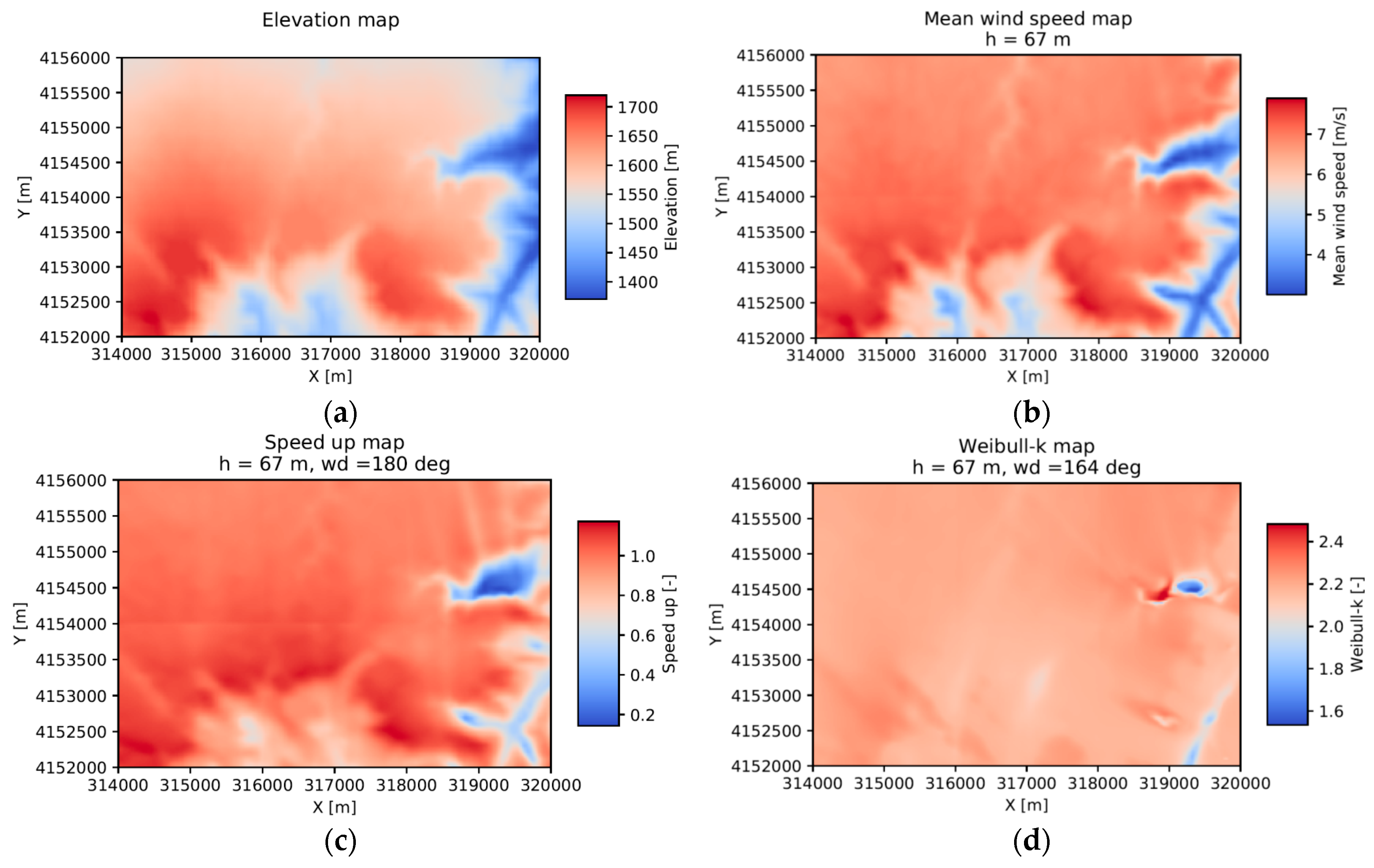
Considering a rectangle area covering the interested area for a wind farm design, we first discretize the area into a number of grids, defined by a range of $x$ coordinates $\left[x_1, x_2, \dots , x_{N_x}\right]$ and a range of $y$ coordinates $\left[y_1, y_2, \dots , y_{N_y}\right]$. For a certain number of wind direction sectors defined by a range of far field inflow wind directions $\left[{\theta }_1^{\infty }, {\theta }_2^{\infty }, \dots , {\theta }_{N_{\theta }}^{\infty } \right]$, we can then obtain the relevant sector wise values of wind resource and terrain effects variables, such as Weibull-A, Weibull-k, frequency, speed up factor, terrain induced turning angle, and mean wind speed, at a given height above the ground. Note that Weibull-A is the scale parameter and Weibull-k is the shape parameter of Weibull distribution, which is the most commonly used distribution for wind speed [4]. Values of variables that do not depend on inflow wind direction, such as elevation and overall mean wind speed, are also obtained.

Using linear interpolation, we can then easily estimate the values of these variables for any arbitrary position $\left(x, y\right)$ in this area, under any far field inflow wind direction, ${\theta }^{\infty }$, if wind direction dependent variables are concerned. The variables important for estimating AEP are listed in

Table 1. Site condition variables important for AEP (annual energy production) estimation.

Variable	Unit	Notation
Elevation	m	$z\left(x, y\right)$
Weibull-A	m/s	$A\left(x, y,{\theta }^{\infty }\right)$
Weibull-k	-	$k\left(x, y,{\theta }^{\infty }\right)$
Frequency	-/°	$freq\left(x, y,{\theta }^{\infty }\right)$
Speed up	-	$sp\left(x, y,{\theta }^{\infty }\right)$
Turning angle	°	$tu\left(x, y,{\theta }^{\infty }\right)$

.

In Table 1, speed up is defined as the ratio between the local wind speed, $v$, at location $\left(x, y\right)$ and the far field wind speed, $v^{\infty }$, at the same height above the ground for a given far field inflow wind direction, ${\theta }^{\infty }$, while turning angle, $tu$, denotes the difference between the local wind direction, $\theta$, and the far field inflow wind direction, ${\theta }^{\infty }$. Thus, they can be computed as:

$$sp\left(x, y,{\theta }^{\infty }\right)=v\left(x, y,{\theta }^{\infty }\right)/v^{\infty }\left({\theta }^{\infty }\right),$$

(1)

$$tu\left(x, y,{\theta }^{\infty }\right)=\theta \left(x, y,{\theta }^{\infty }\right)-{\theta }^{\infty }.$$

(2)

As a demonstration, four interpolated site condition variables are shown in Figure 1 for a real wind farm site in complex terrain. Note that the results on wind resource and terrain effects are imported from WAsP CFD simulations and the wind farm on this site will be used in Section 4 and Section 5 as a test case.

2.2. Wake Model

Modelling the wake effects of wind turbines is essential for AEP estimation, but quite challenging for wind farms in complex terrain due to the complex interplay between terrain and wake flow [22]. While the CFD can model the wake flow field of a wind farm in complex terrain with a reasonable accuracy [23], its high computational cost makes it unsuitable for wind farm design optimization, since typical optimization algorithms require a large number of design evaluations.

Several studies have proposed a few fast wake models for wind farms in complex terrain: Song et al. proposed a virtual particle wake model [24] and applied it in wind farm layout optimizations [12,13]; Feng and Shen developed an adapted Jensen wake model in [14]; Kuo et al. [25] proposed a wake model by solving a simplified variation of the Navies-Stokes equations, which yields results with a reasonable accuracy and has a much less computational cost when compared with full CFD simulations.

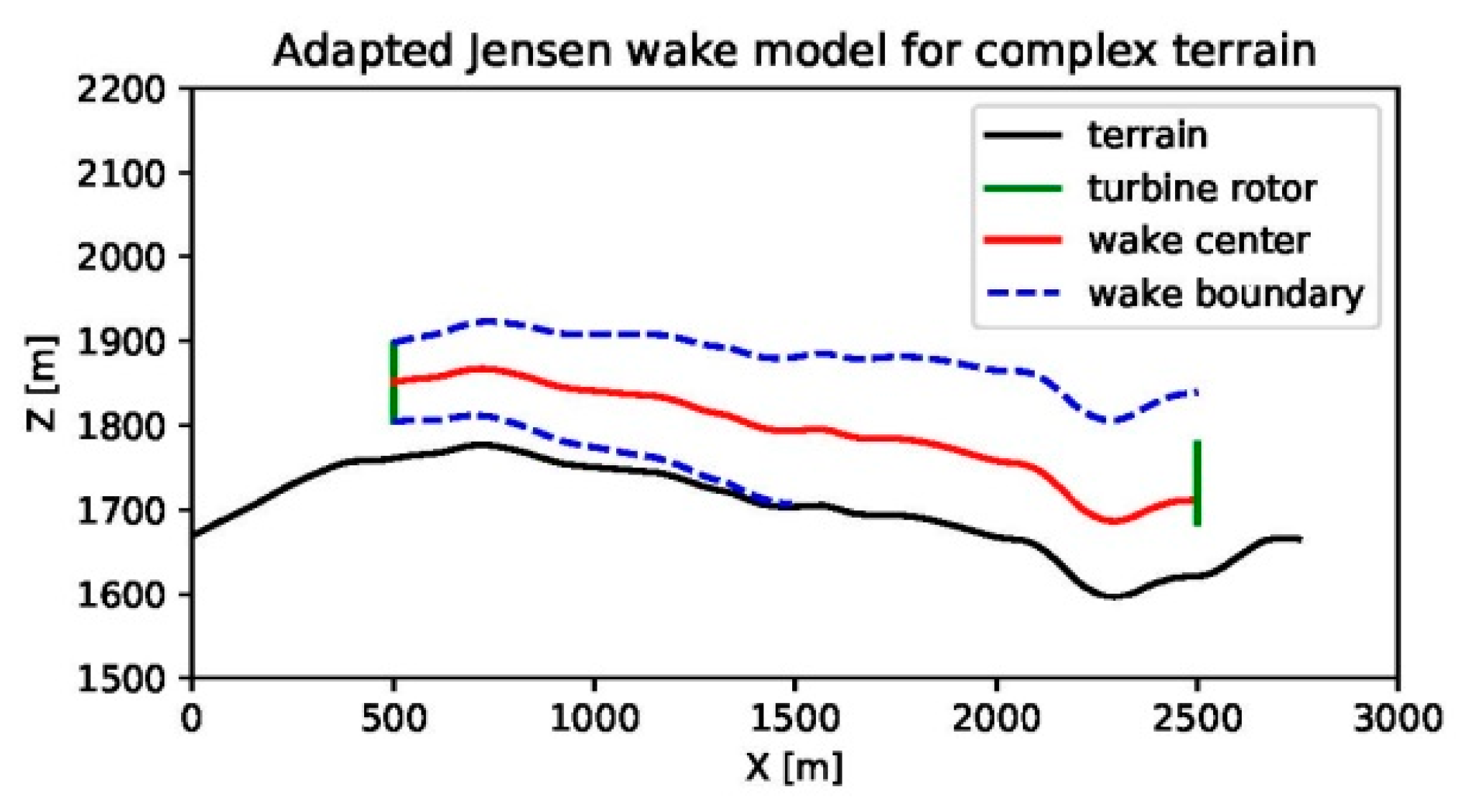
In the current framework, the wake flow field of a wind farm in complex terrain is modelled by coupling the adapted Jensen wake model with the terrain flows obtained by CFD simulations, i.e., flow fields of the wind farm site without wind turbines, such as those imported from WAsP CFD simulations. The adapted Jensen wake model assumes the wake centerline of a wind turbine’s wake follows the terrain at the same height above the ground along the local inflow wind direction, while its wake zone expands linearly and its wake deficit develops following the same rule as the original Jensen wake model [14]. The schematic of this wake model is shown in Figure 2.

Considering the wake effect between an upwind turbine, $i$, located at $(x_i, y_i)$ and a downwind turbine, $j$, located at $(x_j, y_j)$ for a given far field inflow condition: $v^{\infty }$ and ${\theta }^{\infty }$, we can calculate the downwind distance, $d_{ij}^{down}\left({\theta }^{\infty }\right)$, and the crosswind distance, $d_{ij}^{cross}\left({\theta }^{\infty }\right)$, from the upwind turbine to the location of the downwind turbine. The downwind distance can be computed by integration following the wake centerline (the red line in Figure 2) based on the elevation, $z\left(x, y\right)$, and the local inflow wind direction, ${\theta }_i\left({\theta }^{\infty }\right)={\theta }^{\infty }+tu\left(x_i, y_i,{\theta }^{\infty }\right)$, while the crosswind distance can be easily obtained by considering the coordinates of these two turbines and the local inflow wind direction of the upwind turbine. Then, the local inflow wind speed at turbine $i$ and the effective wake deficit turbine $i$ caused on turbine $j$ can be calculated by:

$$v_i\left(v^{\infty },{\theta }^{\infty }\right)=sp\left(x_i, y_i,{\theta }^{\infty }\right)·v^{\infty },$$

(3)

$$\Delta v_{ij}\left(v^{\infty },{\theta }^{\infty }\right)=\frac{A_{ij}^{ol}\left({\theta }^{\infty }\right)}{A_j^{rotor}}·v_i\left(v^{\infty },{\theta }^{\infty }\right)·\left(\frac{1-\sqrt{1-C_T\left(v_i\left(v^{\infty },{\theta }^{\infty }\right)\right)}}{1+\alpha ·d_{ij}^{down}\left({\theta }^{\infty }\right)/R_i}\right),$$

(4)

in which $A_{ij}^{ol}\left({\theta }^{\infty }\right)$ is the overlapping area between the wake zone of turbine $i$ and the rotor area of turbine $j$; $A_j^{rotor}=\pi R_j^2$ is the rotor area of turbine $j$; $C_T(·)$ represents the thrust coefficient function of the wind turbine; $\alpha$ denotes the wake decay coefficient, and $R_i$ represents the rotor radius of turbine $i$. Note that $A_{ij}^{ol}\left({\theta }^{\infty }\right)$ can be calculated based on the wake zone radius, $R_{wake}=R_i+ \alpha ·d_{ij}^{down}\left({\theta }^{\infty }\right)$, the rotor radius, $R_j$, and the relevant crosswind distance, $d_{ij}^{cross}\left({\theta }^{\infty }\right)$, using the method described in [14]. Additionally, $\alpha =0.075$ is used in this study.

Denoting the set of indexes of all the turbines upwind of turbine $j$ as $I^{up}$, and using the energy deficit balance assumption [14], we can then calculate the effective wind speed of turbine $j$ under the far field inflow wind condition, $v^{\infty }$ and ${\theta }^{\infty }$, as:

$${\overline{v}}_j\left(v^{\infty },{\theta }^{\infty }\right)=v_j\left(v^{\infty },{\theta }^{\infty }\right)-\sqrt{{\sum }_{i\in I^{up}}{\left(\Delta v_{ij}\left(v^{\infty },{\theta }^{\infty }\right)\right)}^2}.$$

(5)

A more detailed description of the wake model governed by Equations (3)–(5) is referred to in [14].

2.3. AEP Estimation

After the local wind speeds with and without wake effects of each wind turbine are obtained by using Equations (3)–(5), it is then easy to calculate the corresponding power outputs using the power curve of the wind turbine.

Note that the site condition described in Section 2.1 provides wind resource parameters at each turbine site for a given far field inflow wind direction, i.e.,: $A_i\left({\theta }^{\infty }\right)=A\left(x_i, y_i,{\theta }^{\infty }\right)$, $k_i\left({\theta }^{\infty }\right)=k\left(x_i, y_i,{\theta }^{\infty }\right)$ and $fre{q}_i\left({\theta }^{\infty }\right)=freq\left(x_i, y_i,{\theta }^{\infty }\right)$. Based on these parameters, the probability of each turbine site’s local wind condition, i.e., $v_i\left(v^{\infty },{\theta }^{\infty }\right)$ and ${\theta }_i\left({\theta }^{\infty }\right)$, with respect to the far field inflow wind condition ($v^{\infty }$ and ${\theta }^{\infty }$) can be estimated by using the joint distribution proposed in [26] as:

$$\begin{array}{cc}\hfill pd{f}_i\left(v^{\infty },{\theta }^{\infty }\right)=& pdf\left(v_i\left(v^{\infty },{\theta }^{\infty }\right), {\theta }_i\left({\theta }^{\infty }\right)\right)\hfill \\ & =\frac{k_i\left({\theta }^{\infty }\right)}{A_i\left({\theta }^{\infty }\right)}·{\left(\frac{v_i\left(v^{\infty },{\theta }^{\infty }\right)}{A_i\left({\theta }^{\infty }\right)}\right)}^{k_i\left({\theta }^{\infty }\right)-1}·\exp \left(-{\left(\frac{v_i\left(v^{\infty },{\theta }^{\infty }\right)}{A_i\left({\theta }^{\infty }\right)}\right)}^{k_i\left({\theta }^{\infty }\right)}\right)·fre{q}_i\left({\theta }^{\infty }\right)\hfill \end{array}$$

(6)

Thus, for a wind farm composed of $N_{wt}$ turbines, its gross and net AEP, i.e., AEP with and without wake effects, can be estimated as:

$${\mathrm{AEP}}_{gross}={\displaystyle \sum }_{i=1}^{N_{wt}}8760·{\eta }_i·\iint P\left(v_i\left(v^{\infty },{\theta }^{\infty }\right)\right)·pd{f}_i\left(v^{\infty },{\theta }^{\infty }\right)d{v}^{\infty }{\theta }^{\infty },$$

(7)

$${\mathrm{AEP}}_{net}={\displaystyle \sum }_{i=1}^{N_{wt}}8760·{\eta }_i·\iint P\left({\overline{v}}_i\left(v^{\infty },{\theta }^{\infty }\right)\right)·pd{f}_i\left(v^{\infty },{\theta }^{\infty }\right)d{v}^{\infty }{\theta }^{\infty },$$

(8)

in which 8760 is the total number of hours in a year, ${\eta }_i$ denotes the availability factor of turbine $i$, and $P(·)$ represents the power curve of the wind turbine. The integrations in Equations (7) and (8) are done numerically after properly discretizing the interested ranges of $v^{\infty } \mathrm{and} {\theta }^{\infty }.$ In this study, the availability factors of all the turbines are assumed to be 1.0 and the discretization used in numerical integration is $\Delta v^{\infty }=1$ m/s, and $\Delta {\theta }^{\infty }=$5°.

3. Optimization Framework

3.1. Problem Formulation

For a wind farm with $N_{wt}$ turbines, its design can be specified by the turbines’ locations, i.e., $\mathit{X}=\left[x_1, x_2, \dots , x_{N_{wt}}\right]$ and $\mathit{Y}=\left[y_1, y_2, \dots , y_{N_{wt}}\right]$. Then, a general optimization problem of the wind farm design can be formulated as:

$$\begin{array}{ccc}\min & f_m\left(\mathit{X},\mathit{ }Y\right),\hfill & m=1,2,\dots ,M,\hfill \\ \mathrm{subject} \mathrm{to}:& g_k\left(\mathit{X}, \mathit{Y}\right)\ge 0,\hfill & k=1,2,\dots , K;\hfill \\ & {\mathit{X}}^{\left(L\right)}\le \mathit{X}\le {\mathit{X}}^{\left(U\right)};& \\ & {\mathit{Y}}^{\left(L\right)}\le \mathit{Y}\le {\mathit{Y}}^{\left(U\right)}.& \end{array}\}$$

(9)

where $f_m$ is the mth objective function, $g_k$ is the kth inequality constraint function, and ${\mathit{X}}^{\left(L\right)}$, ${\mathit{X}}^{\left(U\right)}$, ${\mathit{Y}}^{\left(L\right)}$, and ${\mathit{Y}}^{\left(U\right)}$ denote the lower and upper bounds.

Common objective functions for wind farm design optimization include AEP, LCOE, profit, noise emission, and so on. Typical constraints that can be modelled as inequality constraint functions include wind farm boundary, exclusive zones, and wind turbine proximity. In the current framework, the default objective function is AEP and the considered constraints are summarized in the next subsection.

3.2. Constraints

Wind farm design is subject to various constraints, which may come from technical, logistical, environmental, economical, legal, and/or even social considerations. In the current framework, three types of constraints are considered: (1) inclusive and exclusive boundaries; (2) minimal distance requirements; and (3) bounds on certain site condition variables.

Inclusive and exclusive boundaries denote the feasible and infeasible area for placing turbines, which may come from limitations and requirements on leased land, existing roads and properties, soil conditions, and so on. As a general method, polygons can be used to model inclusive and exclusive zones defined by the inclusive and exclusive boundaries. Thus, for a wind farm with $N_{inc}$ inclusive and $N_{exc}$ exclusive boundaries, the individual inclusive and exclusive zones and the overall feasible zone can be modeled as:

$$\begin{array}{cc}{S}_{inc}^i=\left\{\left(x, y\right)|\begin{array}{cc}{a}_k^{i}x+b_k^{i}y\le c_k^i,& k=1,2, \dots , m^i\end{array}\right\},& i=1,2, \dots , N_{inc}\end{array}$$

(10)

$$\begin{array}{cc}{S}_{exc}^j=\left\{\left(x, y\right)|\begin{array}{cc}{a}_l^{j}x+b_l^{j}y\le c_l^j,& l=1,2, \dots , n^j\end{array}\right\},& j=1,2, \dots , N_{exc}\end{array}$$

(11)

$$S_{\mathrm{feasible}}=\left\{\left(x, y\right)|\begin{array}{cc}\left(x, y\right)\in {\cup }_{i=1}^{N_{\mathrm{inc}}}{S}_{inc}^i,& \left(x, y\right)\notin {\cup }_{j=1}^{N_{\mathrm{exc}}}{S}_{exc}^j\end{array}\right\}$$

(12)

where $m^i$ and $n^j$ are the polygon edge numbers of the ith inclusive and jth exclusive boundaries, respectively.

Thus, the constraints on inclusive and exclusive boundaries of the wind farm design can be written as:

$$\begin{array}{cc}(x_i, y_i)\in S_{\mathrm{feasible}},& \mathrm{for} i=1,2, \dots , N_{\mathrm{wt}}.\end{array}$$

(13)

The second type of constraint is also typical in the engineering practice, which requires the distance between any two turbines larger than a minimal value. This is because a shorter distance between turbines will give a larger wake loss and a higher turbulence intensity, which results in a higher level of fatigue loads and maintenance cost, and even a shorter lifetime of turbines. Also, a minimal distance is required to make sure two turbines’ blades never contact each other and one turbine never falls on the other turbine. In the current framework, a fixed minimal distance requirement, $Dis{t}_{\min }$, is assumed for any two turbines. Thus, the constraints on the minimal distance requirement are governed by:

$$\begin{array}{cc}\sqrt{{\left(x_i-x_j\right)}^2+{\left(y_i-y_j\right)}^2}-Dis{t}_{\min }\ge 0& \mathrm{for} i,j=1,2, \dots , N_{\mathrm{wt}} \mathrm{and} i\ne j.\end{array}$$

(14)

The third type of constraints exposes requirements on certain site condition variables to rule out certain unfavorable sites, such as those with too low a mean wind speed, too high a turbulence intensity, or too rugged terrain. When applied properly, this type of constraint can help the optimizer to focus on the more favorable design space and speed up the convergence process, as found in [18].

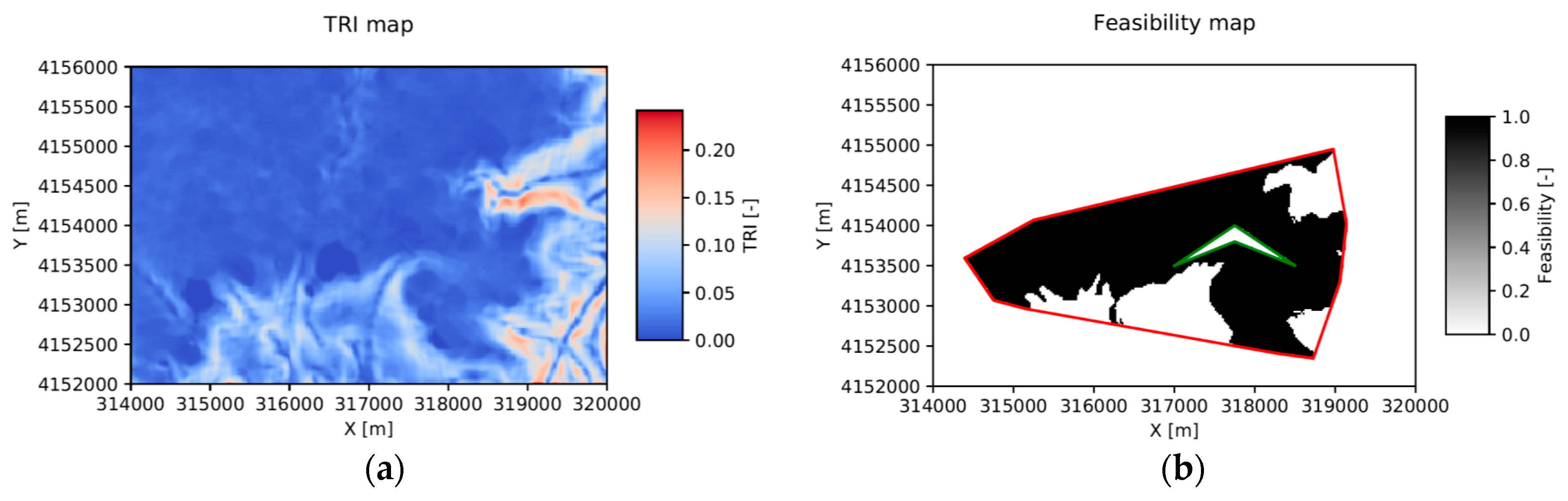
To measure the degree of the terrain ruggedness, a terrain ruggedness index (TRI) is introduced. This index was first proposed by Riley et al. [27] as a quantitative measure of topographic heterogeneity. A dimensionless version of this index is developed in the current framework, which can be calculated based on the elevation data of grids as defined in Section 2.1. Given the grid sizes along the $x$ and $y$ directions are $\Delta x$ and $\Delta y$, the TRI at grid $(x_i, y_j)$ can be computed based on its elevation and the elevation values of the eight surrounding grids as:

$$\begin{gathered} \mathrm{TRI}(x_i, y_j)= \frac{1}{8}\{\frac{{\left[\mathrm{z}(x_i, y_j)-\mathrm{z}(x_{i+1}, y_j)\right]}^2}{\Delta x^2}+\frac{{\left[\mathrm{z}(x_i, y_j)-\mathrm{z}(x_{i-1}, y_j)\right]}^2}{\Delta x^2} \\ +\frac{{\left[\mathrm{z}(x_i, y_j)-\mathrm{z}(x_i, y_{j+1})\right]}^2}{\Delta y^2} +\frac{{\left[\mathrm{z}(x_i, y_j)-\mathrm{z}(x_i, y_{j-1})\right]}^2}{\Delta y^2}+\frac{{\left[\mathrm{z}(x_i, y_j)-\mathrm{z}(x_{i+1}, y_{j+1})\right]}^2}{\Delta x^2+\Delta y^2} \\ +\frac{{\left[\mathrm{z}(x_i, y_j)-\mathrm{z}(x_{i+1}, y_{j-1})\right]}^2}{\Delta x^2+\Delta y^2}{+\frac{{\left[\mathrm{z}(x_i, y_j)-\mathrm{z}(x_{i-1}, y_{j+1})\right]}^2}{\Delta x^2+\Delta y^2}+\frac{{\left[\mathrm{z}(x_i, y_j)-\mathrm{z}(x_{i-1}, y_{j-1})\right]}^2}{\Delta x^2+\Delta y^2}\}}^{1/2} \end{gathered}$$

(15)

For the wind farm site in Figure 1a, the TRI map calculated in Equation (15) is shown in Figure 3a. Note that the grid sizes are chosen as $\Delta x=\Delta y=25 \mathrm{m}$ in this study according to the default setting of WAsP, which makes the total number of grids in the rectangle area shown in Figure 1 as 38,801. In the current framework, the constraints on TRI and mean wind speed, $v^{mean}$, are considered. Note that the mean wind speed values on the grids, $v^{mean}(x_i, y_j)$, can be imported from wind resource assessment tools or calculated based on the sector wise wind resource parameters, i.e., Weibull-A, Weibull-k, and frequency. For an arbitrary site, linear interpolation is used to find the value of TRI and $v^{mean}$. Thus, constraints on TRI and mean wind speed can be written as:

$$\begin{array}{cc}{\mathrm{TRI}}_{max}-\mathrm{TRI}(x_i, y_i)\ge 0,& \mathrm{for} i=1,2, \dots , N_{\mathrm{wt}}, \end{array}$$

(16)

$$\begin{array}{cc}{v}^{mean}(x_i, y_i)-v_{min}^{mean}\ge 0,& \mathrm{for} i=1,2, \dots , N_{\mathrm{wt}}.\end{array}$$

(17)

where ${\mathrm{TRI}}_{max}$ is the allowed maximal TRI and $v_{min}^{mean}$ is the allowed minimal mean wind speed.

For the wind farm site in Figure 1, the feasibility of each grid, $(x_i, y_j)$, can then be estimated as $F(x_i, y_j)$ based on the first and third types of constraints, i.e., constraints defined in Equations (13), (16) and (17). Note that $F(x_i, y_j)$, with a value of 1 (true) or 0 (false), means whether the given site, $(x_i, y_j)$, is a feasible site to install a turbine, i.e., a site satisfies the constraints on inclusive/exclusive boundaries and bounds of certain site condition variables. The map of $F(x_i, y_j)$ is shown in Figure 3b. Note that the black area in this figure denotes the feasible area. Compared with the feasible area defined by Equations (13) and (14), the bounds on TRI and $v^{mean}$ help to reduce the feasible grids from 12,150 to 9218, representing a 24.13% reduction in the feasible design space. This reduction can help certain optimization algorithms, such as RS, to limit the search space and converge faster.

3.3. Optimization Algorithm

To solve the optimization problem, the Random Search (RS) algorithm is used in the current framework. This algorithm was first proposed by Feng and Shen in [15] and improved in [16]. Recently, they also extended the algorithm to cover multiple objective cases [28] and overall design cases with multiple types of turbines [19], and to maximize the robustness of wind farm power production under wind condition uncertainties [29]. It has shown a superior performance when compared to other popular algorithms, such as GA (genetic algorithm) [16], NSGA-II (Non-dominated Sorting Genetic Algorithm II) [28], and mixed-discrete PSO (Particle Swarm Optimization) [19].

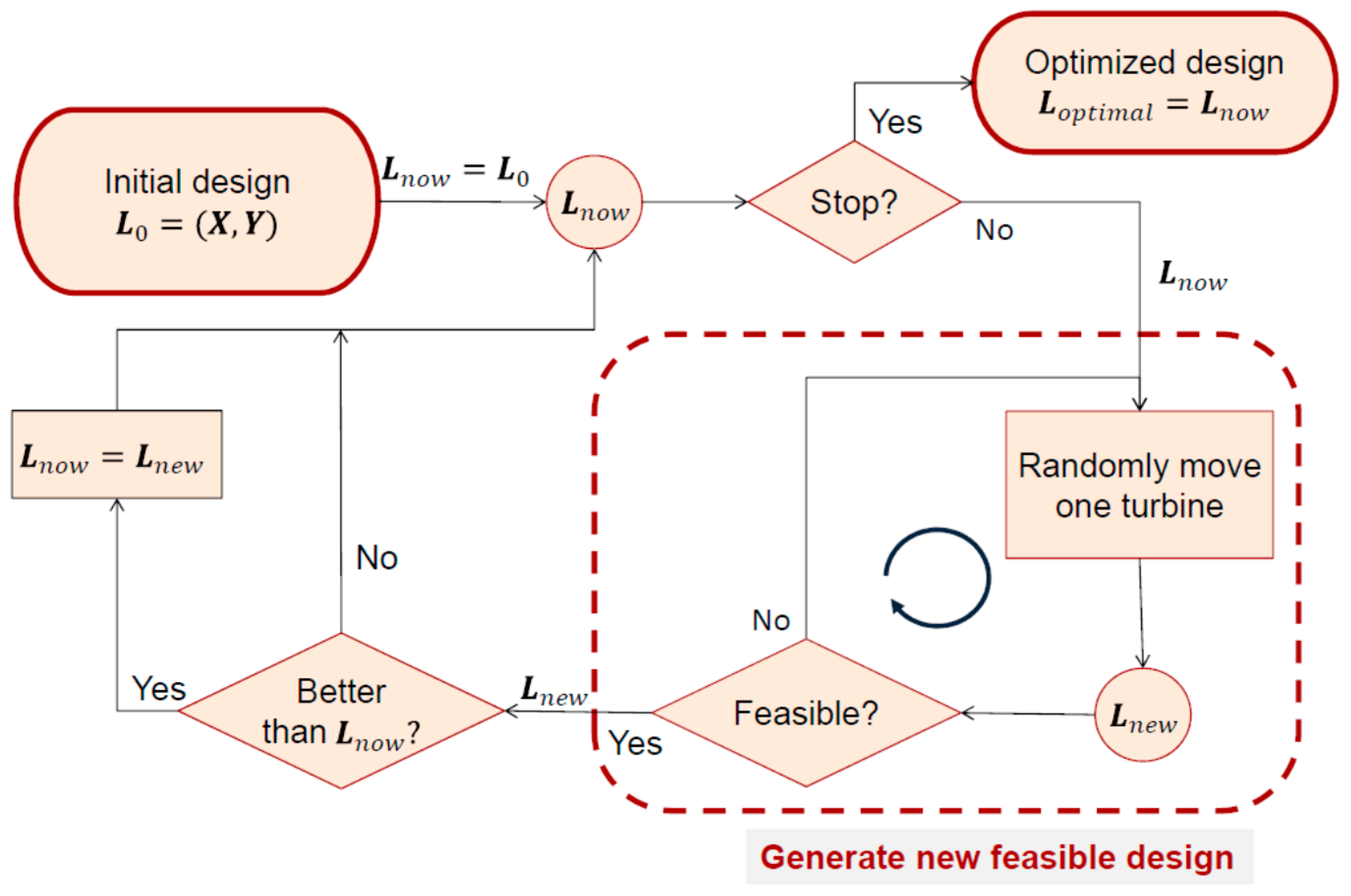
RS is a single solution search method. At each step, a new feasible design, i.e., a design satisfies all the constraints and bounds, is generated by slightly changing the current design, i.e., randomly choosing a turbine and moving it to a random position inside the feasible area. This new design is then compared with the current design with respect to the objective function. If the new design is better, it becomes the current design. If not, the current design remains unchanged. This step is iteratively repeated until a given stop condition is met. Normally, the stop condition can be set as a maximal number of steps (equivalent to the number of objective function evaluations). The procedure of this algorithm is shown as a flowchart in Figure 4.

There are two parameters controlling the RS algorithm: maximal step size, $M_{\max }$, which controls how far away a chosen turbine can be possibly moved from its current position; and maximal number of evaluations, $E_{\max }$, which defines when to terminate the optimization process. $M_{\max }$ should be set large enough to allow the algorithm to explore the design space more thoroughly and escape local minima more likely. When no trials and experimentations are first applied, $M_{\max }$ could be set in the order of the maximal distance between any two points in the feasible wind farm area and $E_{\max }$ should be in the range of 1000 to 10,000.

Due to the randomness involved in the optimization process, meta-heuristics, such as RS, exhibits a stochastic nature, meaning different runs typically obtain different results. This also means that the quality of the initial solution(s) can have profound influences on the final optimization results and the convergence speed [30]. Saavedra-Moreno et al. [31] tackled this problem by seeding an evolutionary algorithm with initial solutions obtained by a greedy heuristic algorithm, and applied this method in wind farm layout optimization.

In this study, a simple algorithm called Heuristic Fill is proposed to find a good initial design, based solely on site conditions and constraints. As described in Section 3.2, the feasibility of each grid, $(x_i, y_j)$, can be calculated as $F(x_i, y_j)$ based on constraints defined in Equations (13), (16), and (17). The mean wind speed of each grid, $v^{mean}(x_i, y_j)$, can also be obtained from site conditions. The algorithm then tries to fill the feasible grids with $N_{\mathrm{wt}}$ wind turbines one by one according to the corresponding mean wind speed from high to low, while respecting the minimal distance constraints in Equation (14). This algorithm can be summarized in the pseudo code shown in Algorithm 1.

Algorithm 1. Pseudo code of the Heuristic Fill algorithm.

(1) Find the set of feasible grid points: $G_{feasible}=\left\{(x_i, y_j) |F(x_i, y_j)=1, \mathrm{for} i=1, 2, \dots , N_x, j=1, 2, \dots , N_y\right\}$; (2) Sort the feasible grid points according to mean wind speed, i.e., find a list of feasible grid points as $\left[(x_{i^1}, y_{j^1}),(x_{i^2}, y_{j^2}),\dots ,(x_{i^m}, y_{j^m}), \right]$, where $(x_{i^k}, y_{j^k})\in G_{feasible}$ with $k=1,2, \dots , m$ and $v^{mean}(x_{i^k}, y_{j^k})\ge v{v}^{mean}(x_{i^{k+1}}, y_{j^{k+1}})$ with $k=1, 2, \dots , m-1$; (3) Heuristically fill with $N_{\mathrm{wt}}$ turbine sites: (a) Set $w=1$, $g=1$; (b) While$1<w\le N_{\mathrm{wt}}$ and $\sqrt{{\left(x_i-x_{i^{\mathrm{g}}}\right)}^2+{\left(y_i-{\mathrm{y}}_{j^{\mathrm{g}}}\right)}^2}<Dis{t}_{\min }$ holds for $i=1,\dots , w-1$:                      $g=g+1$ End While Set $x_w=x_{i^{\mathrm{g}}}$, $y_{\mathrm{w}}={\mathrm{y}}_{j^{\mathrm{g}}}$, $g=g+1$, $w=w+1$; (c) Set the initial layout as $\mathit{X}=[x_{\mathrm{w}}|w=1, 2, \dots , N_{\mathrm{wt}}]$, $\mathit{Y}=\left[y_{\mathrm{w}}|w=1, 2, \dots , N_{\mathrm{wt}}\right]$.

3.4. Framework

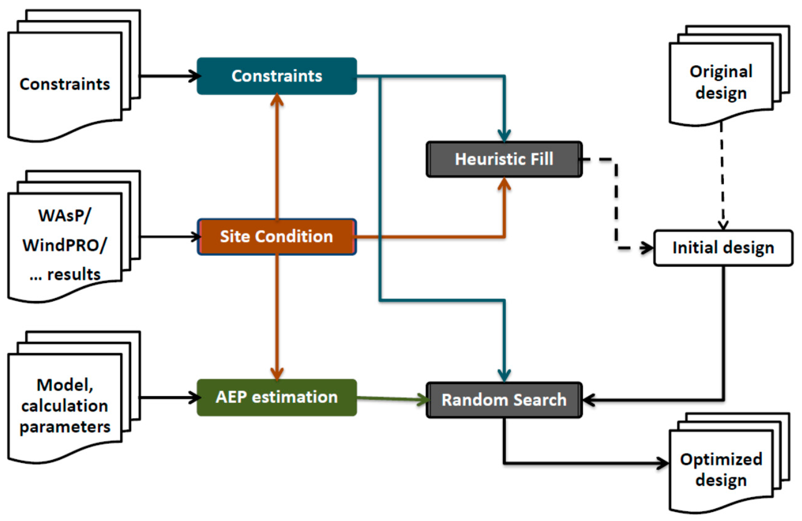
Putting things together, we can describe the framework in the architecture diagram shown in Figure 5. Note that WAsP (or another wind resource assessment code) needs to be used only once to get the relevant results for defining the site conditions, since the wake modelling and AEP estimation, as well as the modelling of constraints and optimization process, are all implemented by the modules inside the framework as introduced in the previous subsections. Thus, this framework can work as a stand-alone tool for wind farm design optimization. If objective functions other than AEP and more constraints are considered, the relevant modules can also be extended accordingly, while the optimization algorithm and the architecture remain unchanged.

4. Case Study and Results

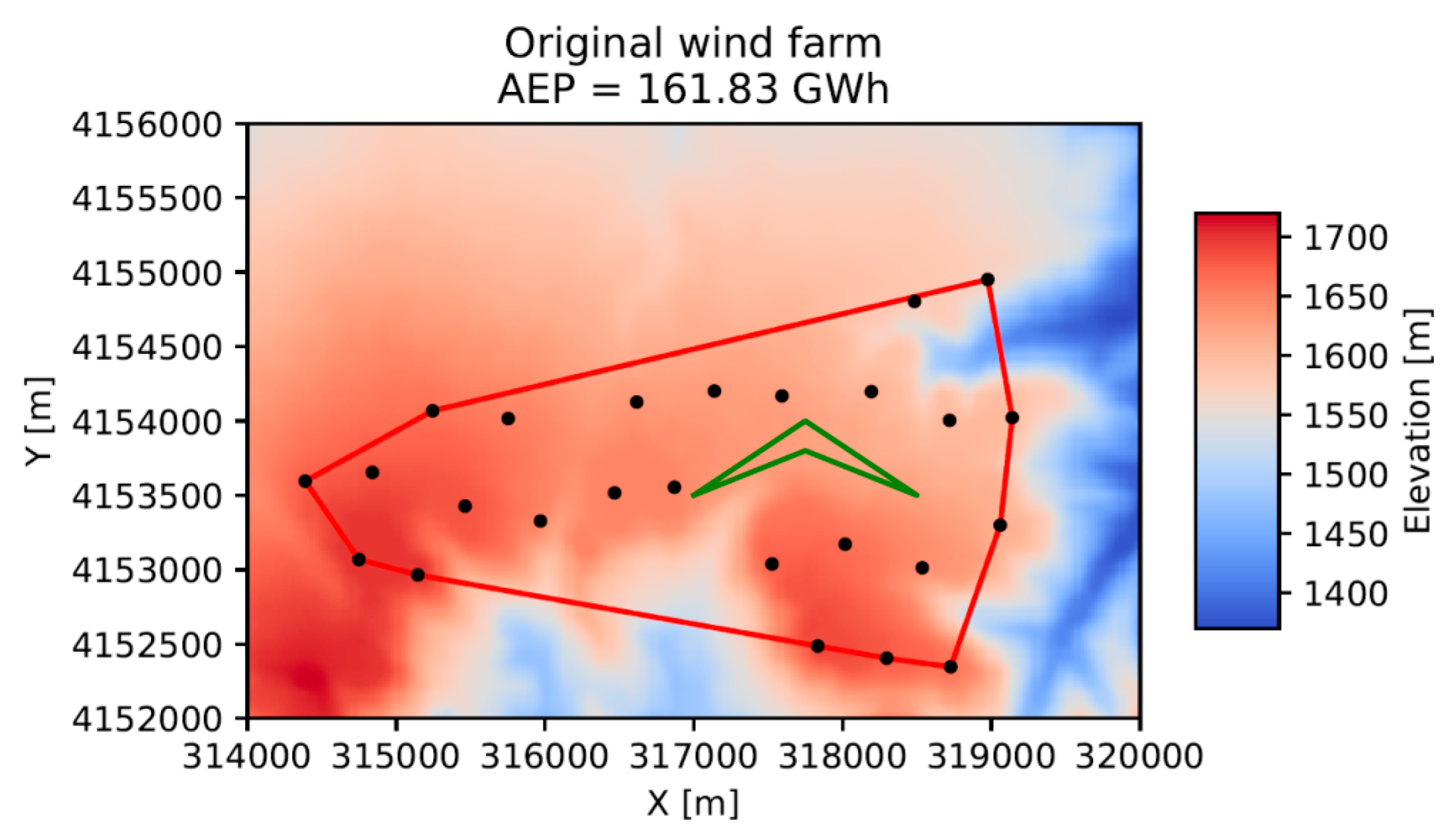
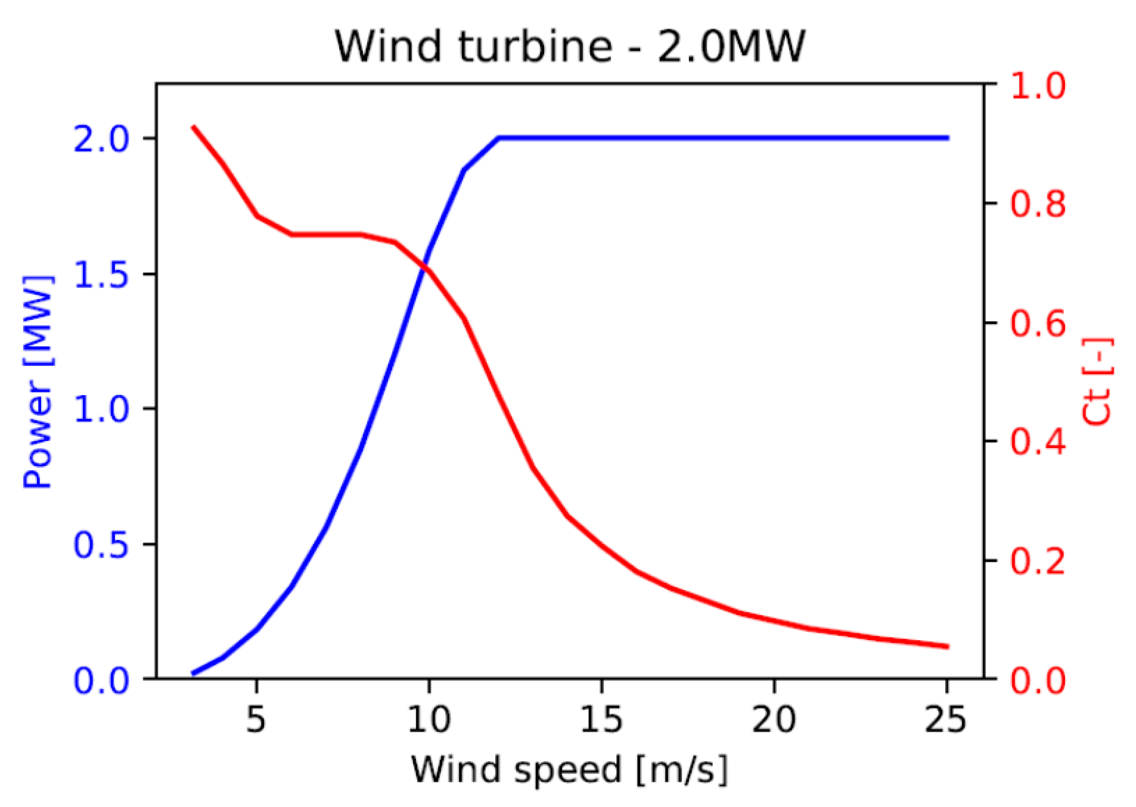
As a demonstration, a case study for an anonymous wind farm in complex terrain using the proposed framework is presented here. This wind farm is located in Northwest China, and has a total capacity of 50 MW with 25 turbines. This wind farm has been studied in [23,32] to investigate the wake flow simulation in complex terrain using CFD, and the preliminary results of the layout optimization study of this wind farm have been presented in [18]. Some of this wind farm’s site conditions have already been shown in Figure 1. Its original layout is shown in Figure 6 and the turbine characteristics are shown in Figure 7. This type of turbine is variable speed, pitch regulated and has a rotor diameter of $D=93 \mathrm{m}$ and a hub height of $H=67 \mathrm{m}$. The cut-in, rated, and cut-out wind speeds are 3 m/s, 12 m/s, and 25 m/s, respectively.

Note that constraints on inclusive and exclusive boundaries and bounds on parameters that are considered in this case study are shown in Figure 3. Additionally, the minimal distance requirement used in Equation (14) is chosen as the minimal distance between the turbines in the original layout, which is $D_{min}=403.8 \mathrm{m}$. The inclusive boundary shown with red line in Figure 6 is set as the minimal convex polygon that covers all the turbines, and the exclusive boundary (the green line) is arbitrarily set to test the modelling capacity of the exclusive boundary of the framework. The choice of the inclusive boundary is to make sure the optimized wind farm occupies the same or a smaller area and the required cost of electrical cables and access roads that connect all turbines stays at the same level, so that the comparison of AEP with the original wind farm makes sense.

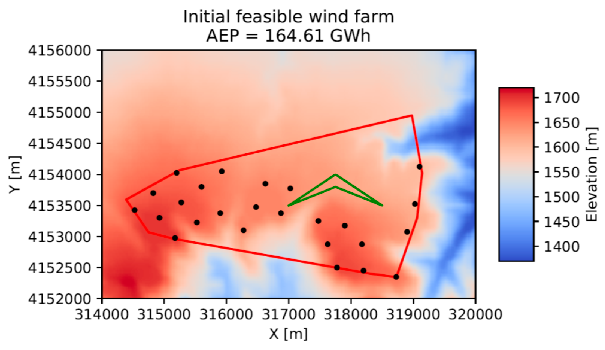
To find a good feasible initial design, the Heuristic Fill algorithm is applied in this wind farm, which obtains an initial design with $\mathrm{AEP}=164.61 \mathrm{GWh}$, as shown in Figure 8.

Compared to the original wind farm, the design found by the Heuristic Fill algorithm obtains an impressive 1.72% increase of AEP (from 161.83 GWh to 164.61 GWh). Note that this increase is achieved by a deterministic filling process without any searching process, thus can be done in several seconds.

To show the performance of the proposed framework, multiple runs of Random Search with different settings of the optimization algorithm are carried out, i.e., optimization runs with different numbers of total evaluation number, $E_{\max }$, and maximal step size, $M_{\max }$. For each of these parameter combinations, 10 optimization runs are done to obtain the statistics. Cases starting from the original design (as shown in Figure 6) and the initial design found by the Heuristic Fill algorithm (as shown in Figure 8) are both tried. The results are summarized in

Table 2. Performance of the framework in multiple runs with different settings.

Opt. Setting		AEP [GWh] (Increase [%])				CPU Time [s]
${\mathit{E}}_{\mathbf{m}\mathbf{a}\mathbf{x}}$ [-]	${\mathit{M}}_{\mathbf{m}\mathbf{a}\mathbf{x}} \left[\mathit{m}\right]$	Initial	Opt. min	Opt. mean	Opt. max	Mean
1000	5000	161.83	164.62 (1.72)	165.03 (1.98)	165.67 (2.37)	2137.5
1000	50	164.61	165.18 (2.07)	165.27 (2.12)	165.30 (2.14)	1824.6
1000	500	164.61	165.17 (2.06)	165.28 (2.13)	165.41 (2.21)	1923.7
1000	5000	164.61	165.17 (2.06)	165.45 (2.24)	165.79 (2.45)	2272.3
5000	5000	164.61	165.76 (2.42)	166.02 (2.58)	166.17 (2.68)	12,042.6
10,000	5000	164.61	165.95 (2.55)	166.11 (2.64)	166.21 (2.70)	24,613.0

. Note that the percentages of AEP that increase in the optimized wind farm design compared to the original wind farm (161.83 GWh) are marked with underlines inside the parentheses, and the CPU time shown here is the mean value per run for 10 runs by a Python 3.6 implementation of the framework on a laptop with an Intel^® i5-2520M CPU @2.50 GHz.

As shown in Table 2, allowing the optimization process to run longer, i.e., with a larger number of evaluations, generally obtains better results (see the last three rows in Table 2). The other advantage for an optimization process is starting from a better initial design, as the results from the initial design obtained by the Heuristic Fill algorithm are much better than those from the original design using the same optimization setting (see the first and fourth rows of the results in Table 2).

The maximal step size also has an effect on the results, as it controls the degree of change that can be made to the current best design in each step. As discussed in Section 3.3, this parameter should be set large enough to explore the design space more thoroughly and thus find a better solution after a sufficient large number of evaluations. This is supported by the comparison of optimization runs with the same $E_{\max }$, but different $M_{\max }$, as shown in the second to fourth rows of Table 2.

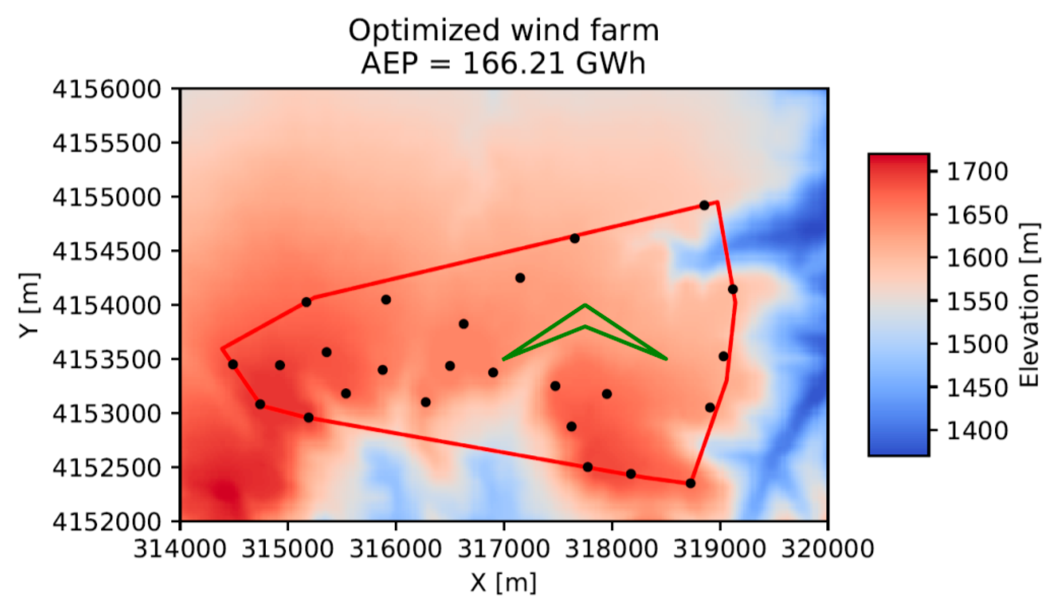
The best optimized design found by all the optimization runs summarized in Table 2 is under the optimization setting: $E_{\max }=10,000$, $M_{\max }=5000 \mathrm{m}$, with the optimized AEP as 166.21 GWh, representing a 2.70% increase to the original wind farm design. This design is found by the Random Search algorithm starting from the initial design obtained by the Heuristic Fill algorithm, and shown in Figure 9.

To better compare the performance of the original, initial, and optimized designs as shown in Figure 6, Figure 8 and Figure 9, their gross and net AEP values are listed in

Table 3. AEP values comparison of the original, initial, and optimized wind farms.

Wind Farm	Net AEP [GWh]	Gross AEP [GWh]	Wake Loss [%]
Original (Figure 6)	161.83	169.75	4.67
Initial (Figure 8)	164.61	175.42	6.16
Optimized (Figure 9)	166.21	174.91	4.97

.

As Table 3 shows, the initial design found by the Heuristic Fill algorithm has both higher gross AEP and higher net AEP than the original design. Although the wake loss is higher for the initial design than the original one (6.16% versus 4.67%), the larger increase (3.34%) of gross AEP thanks to the higher mean wind speed of the sites found by the Heuristic Fill algorithm compensates the higher wake loss and still yields a substantial increase (1.72%) of net AEP. Note that the higher wake loss of the initial design can also be seen from the layout shown in Figure 8, as the turbines are placed much closer to each other than the original layout shown in Figure 6.

Since the optimized design in Figure 9 is obtained by the optimization run starting from the initial design in Figure 8, we can also compare these two designs. Apparently, the optimization algorithm makes a small sacrifice in gross AEP, i.e., allowing the gross AEP to decrease by 0.28% from 175.42 GWh to 174.91 GWh, while decreasing the wake loss percentage from 6.16% to 4.97%. The combined effect allows the optimized design to gain a 0.97% increase of net AEP to the initial design (from 164.61 GWh to 166.21 GWh), representing a 2.70% increase of net AEP when compared to the original design (from 161.83 GWh to 166.21 GWh).

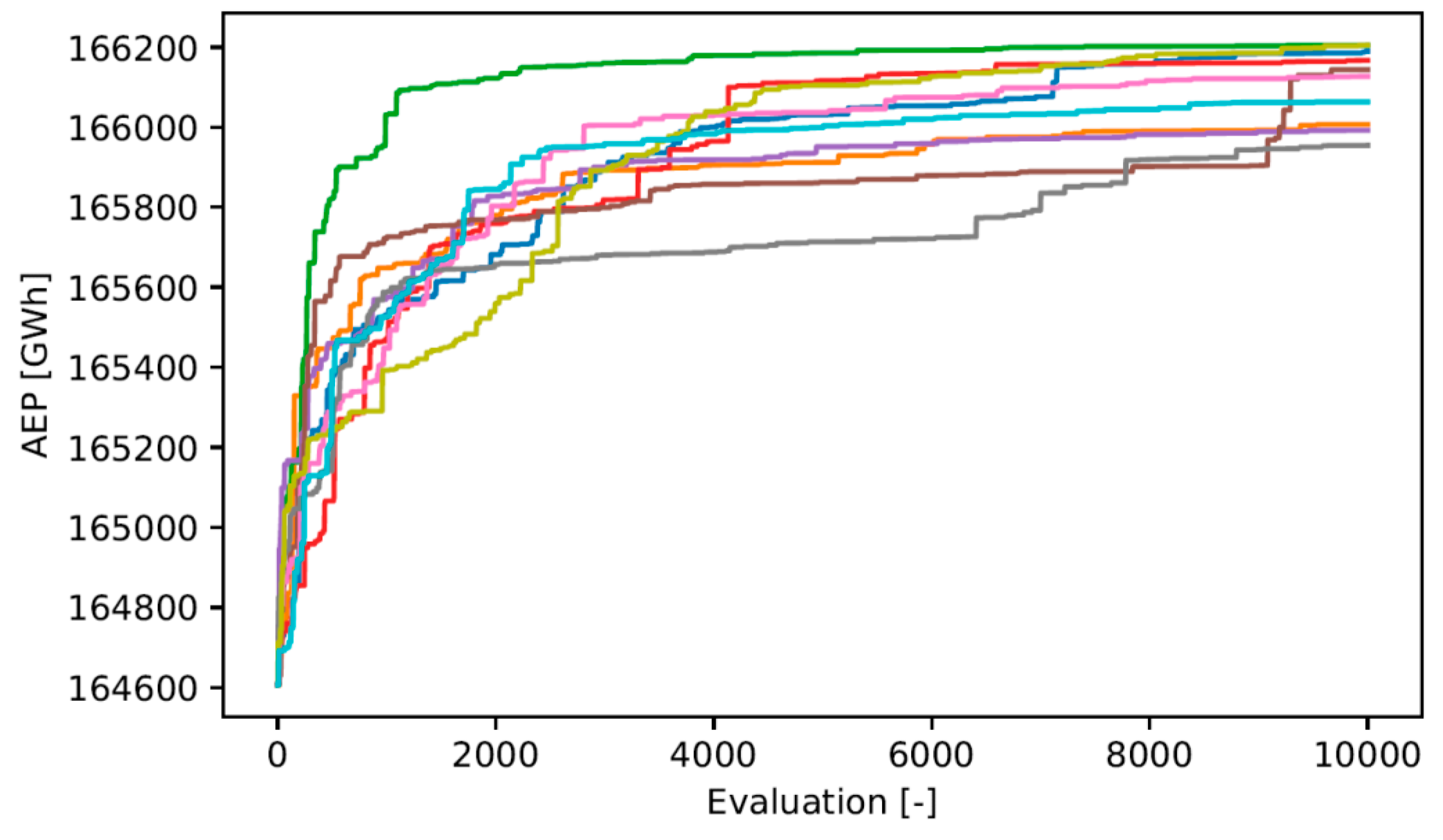
Examining the layout of the initial design in Figure 8 and the layout of the optimized design in Figure 9, we can see that the turbines are scattered away from each other while most of the turbines are still located at high elevation sites. This shows that the optimization algorithm tries to lower wake effects while not sacrifice too much on the gross AEP, as suggested by the net and gross AEP comparison. To show the performance of the framework in multiple runs, the evolution histories of the 10 runs under the optimization setting: $E_{\max }=10,000$, $M_{\max }=5000 \mathrm{m}$ are shown in Figure 10, which demonstrate the random nature of the RS algorithm.

As Figure 10 shows, different runs of the optimization process yield different results. Thus, if it is possible, it is always advised to have multiple runs (10 or more) of the optimization process and use the best result. Also, it is shown for these 10 runs that the largest portion of the AEP increase is achieved in the first 2000 evaluations.

5. Comparison with Other Algorithms

To better show the effectiveness of the RS algorithm for wind farm design in complex terrain, we compare its performance with two widely used algorithms: Particle Swarm Optimization (PSO) and Genetic Algorithm (GA) [33].

PSO is a population based meta-heuristic algorithm inspired by bird flocking, which maintains a population of solutions (called particles) and moves each particle in the design space according to the global best solution in the population and the local best solution found by each particle. In this study, the version of PSO used by Chowdhury et al. in [34] is implemented in Python with the algorithm parameters set as recommended in

Table 4. Performance comparison of three algorithms: PSO (particle swarm optimization), RCGA (real-coded genetic algorithm) and RS (random search).

Initial Scenario	Algorithm	AEP [GWh]			${\mathit{E}}_{\mathbf{m}\mathbf{a}\mathbf{x}}$ [-]
		Worst Initial	Best Initial	Optimized
Random	PSO	119.12	152.44	160.76	5000
	RCGA	119.12	152.44	156.68	5000
	RS	119.12	119.12	173.58	5000
	PSO	119.12	152.44	161.66	50,000
	RCGA	119.12	152.44	165.43	50,000
	RS	119.12	119.12	174.26	10,000
Heuristic fill	PSO	170.27	171.18	171.74	10,000
	RCGA	170.27	171.18	171.96	10,000
	RS	170.27	170.27	174.10	10,000
	PSO	170.27	171.18	171.84	50,000
	RCGA	170.27	171.18	172.58	50,000
	RS	170.27	170.27	173.80	5000

Note: ‘Worst/best initial’ represents the worst/best performing initial solution among the 250 random initial layouts for the random scenario and the 125 seeded good initial layouts for the heuristic fill scenario. These two values are the same for RS as it maintains only one solution. ‘Optimized’ denotes the global best solution found by PSO/RCGA.

of [34]. Details of this algorithm are referred to in the paper [34].

GA is also a nature inspired population based meta-heuristic algorithm for optimization problems. Various versions of GA have been applied to solve the wind farm layout optimization problem, most of which are binary coded [33]. As a binary-coded GA makes restrictions on where to place turbines and thus limits the design space, we choose to implement a real-coded GA (RCGA) recently proposed by Chuang et al. [35], which has no such restrictions. This version of RCGA was developed for constrained optimization based on three specially designed evolutionary operators, i.e., ranking selection, direction-based crossover, and dynamic random mutation, and showed a better performance than traditional versions of RCGA for a variety of benchmark constrained optimization problems [35]. A Python version of this algorithm is implemented in this study using the parameters recommended by the authors of [35]. Details of this algorithm can be found in [35].

For the sake of simplicity, we consider the design optimization problem for the same wind farm as in the case study with only bounds on the design variables, i.e., $x$ and $y$ coordinates of wind turbines. No constraints on wind resource, terrain parameters, and minimal distances are considered. The bounds are set as the boundary of the rectangle area shown in Figure 6, i.e., $314,000 \mathrm{m}\le x\le 320,000 \mathrm{m}$ and $4,152,000 \mathrm{m}\le y\le 4,156,000 \mathrm{m}$. Following the recommendations in [34,35], the size of the population is set as 250 for both PSO and RCGA.

Two scenarios for setting the initial solution(s) are tested. In the random scenario, 250 initial layouts are generated randomly by putting 25 turbines randomly inside the bounds. These initial layouts are used in PSO and RCGA as the initial population, while the worst performing initial layout, i.e., the layout with lowest AEP, is used as the initial solution in RS.

As the initial solution(s) has influences on the optimization results obtained by meta-heuristics, there has been an effort on seeding good initial solution(s) for meta-heuristics in the field of wind farm layout optimization [31]. We address this issue in the heuristic fill scenario. In this scenario, an initial layout is first obtained by using the Heuristic Fill algorithm described in Section 3 with the minimal distance requirement set as four times of the rotor diameter. Then, a group of 124 layouts are generated by running RS 124 times with $E_{\max }=100$ and $M_{\max }=5000 \mathrm{m}$ from the initial layout found by Heuristic Fill. Thus, these 124 initial layouts have a higher or the same AEP as the one found by the Heuristic Fill, as they are improved better ones found by RS. After this process, we have 125 good initial layouts, which are then seeded in the initial populations of PSO and GA, while the remaining halves of the initial populations are filled with random layouts. In this way, the initial populations for both PSO and GA have some good quality initial solutions and some random initial solutions, thus they have a good degree of randomness, which is essential for the diversification. For RS, the worst performing layout among the 125 good initial layouts is used as the initial solution.

The performance of these three algorithms with a different number of evaluations ($E_{\max }$) for both scenarios are summarized in Table 4.

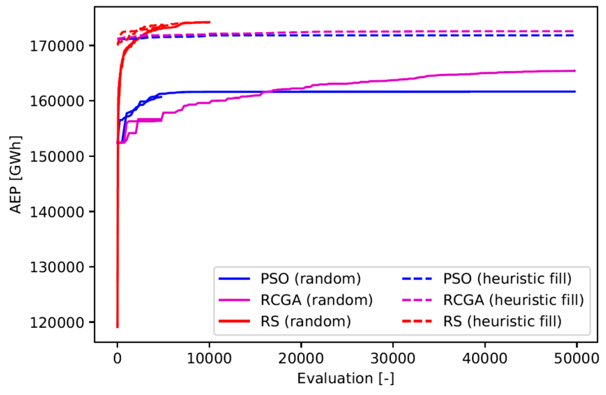
It is worth to note that in both scenarios, RS starts from the worst initial solution among the solutions seeded in the initial population for PSO and GA, thus with a disadvantage in terms of the quality of the initial solution(s). Despite this disadvantage, RS shows a much better performance than PSO and RCGA. As Table 4 shows, RS with 10,000 evaluations obtains the best optimized layout in both scenarios. Compared with PSO and RCGA, RS with only 5000 evaluations largely outperforms PSO and RCGA with 50,000 evaluations (equivalent to 200 generations) in both scenarios, which clearly demonstrates the effectiveness of RS. To better visualize the difference between algorithms, the evolution histories of the best solutions in the different runs of PSO, RCGA, and RS are shown in Figure 11.

Figure 11 shows that: (1) starting from good initial solutions makes PSO and RCGA converge to much better optimized solutions, while its benefit for RS is not so profound; (2) RCGA obtains better results than PSO after a sufficient number of evaluations (20,000); and (3) RS converges faster to a better solution than PSO and RCGA in both scenarios. Based on the results described above, it is natural to conclude that RS used in the current framework performs much better than PSO and RCGA for this case.

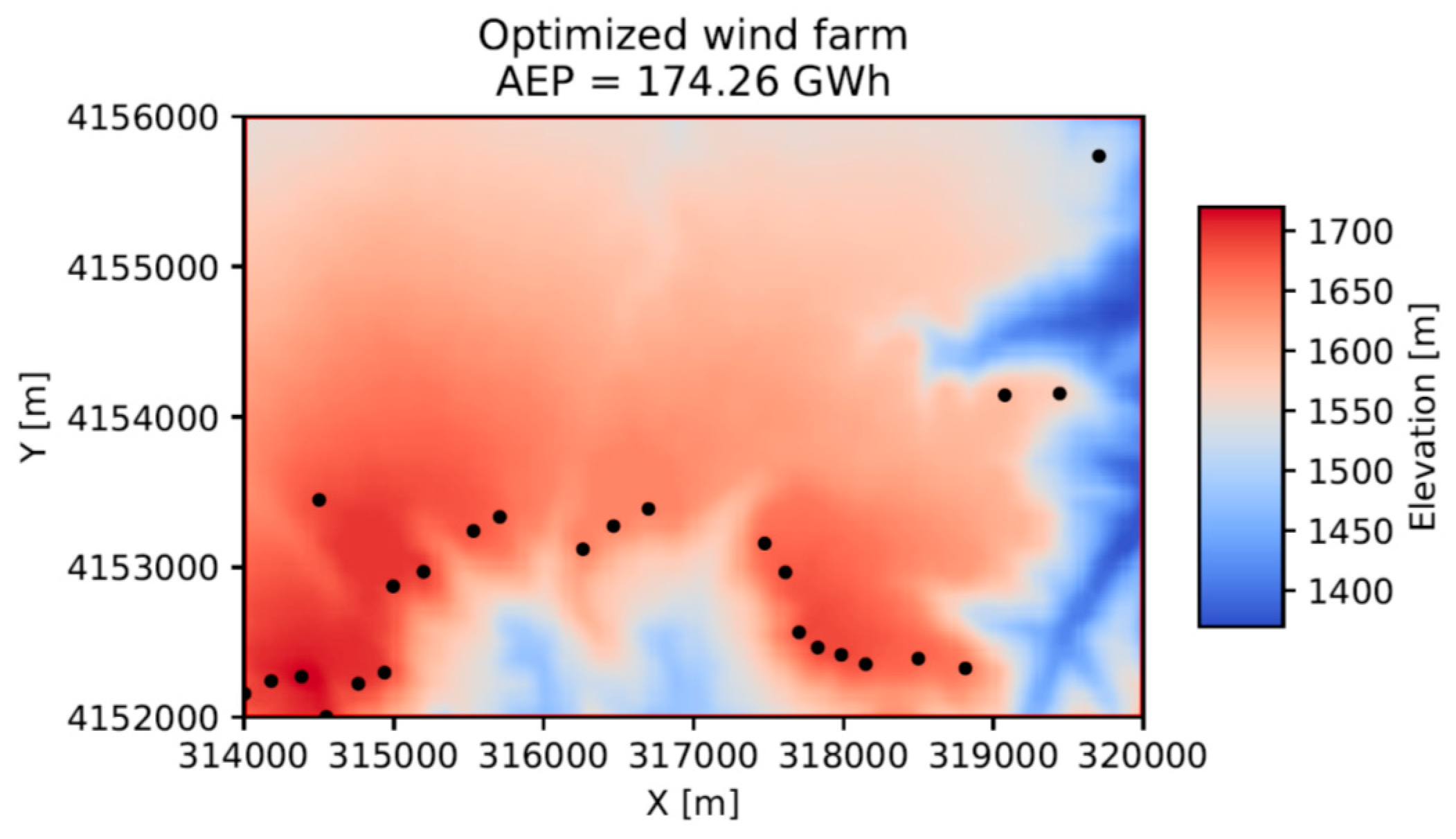
The best optimized design, which is found by RS with 10,000 evaluations in the random scenario, is shown in Figure 12.

Without the limitation of inclusive and exclusive boundaries, the turbines in the optimized design in Figure 12 are spread out in the whole rectangle area and mostly occupying high elevation sites. Note that these sites also have high mean wind speeds as shown in Figure 1b. To place more turbines on the limited high elevation sites, some of the turbines are placed quite close (down to 170.44 m), which could cause problems on fatigue loads for certain turbines. Although the optimized wind farm has a much higher AEP (174.26 GWh), representing a 7.68% increase over the original wind farm, it should be interpreted with caution, as in one aspect, it occupies a much larger area and thus requires more investments on electrical cables and access roads, and in the other aspect, it places several turbines too close, thus it will have difficulty satisfying the requirements on fatigue loads.

6. Conclusions

Wind farm design in complex terrain is a crucial yet challenging task. In this work, we present an overall design optimization framework for tackling this task. This framework combines results from state-of-the-art wind resource assessment tools, such as WAsP CFD, a fast engineering wake model, and an advanced optimization algorithm, to solve the wind farm design optimization problem in complex terrain under various realistic constraints and requirements. This makes the framework a valuable tool that can be used by designers/developers who need to optimize wind farm designs in complex terrain under a real-life scenario.

While the framework in its default setting considers maximizing the total net AEP, its modular architecture makes it easy to be extended to consider other objective function(s). More constraints, requirements, and other optimization algorithms can also be easily implemented and added.

Other contributions of this work include: a terrain ruggedness index (TRI) to characterize the terrain feature and model constraints on the terrain ruggedness; and a fast and simple algorithm called Heuristic Fill to find good initial designs for wind farms in complex terrain, by using a deterministic process based on wind resource considerations and constraints.

The case study of a real wind farm in complex terrain demonstrates the effectiveness of the framework and the performance of proposed algorithms. An impressive increase of net AEP (up to 2.70%) is achieved by using the framework, while respecting realistic constraints on inclusive and exclusive boundaries, minimal mean wind speed, and maximal TRI, and minimal distance constraints between turbines. In comparison with two widely used algorithms (PSO and real-coded GA) for the same wind farm without any constraints, the Random Search algorithm also shows a much better performance in terms of convergence speed and optimization results. This of course demonstrates the advantages of the developed framework and proves the usefulness for wind farm designers/developers.

Although the wind farm design considered in the current framework concerns only the turbine layout, other design variables, such as number, hub height(s), and type(s) of turbines, foundations, access roads, and electrical systems, also play important roles for an overall design optimization of a wind farm. Our future works will investigate these problems and extend the framework in this direction.

References

- GWEC: Global Cumulative Installed Capacity 2001–2017. Available online: http://gwec.net/global-figures/graphs/ (accessed on 7 July 2018).
- GWEC: Global Cumulative and Annual Offshore Wind Capacity End 2017. Available online: http://gwec.net/global-figures/graphs/ (accessed on 7 July 2018).
- Alfredsson, P.H.; Segalini, A. Wind farms in complex terrains: An introduction. Phil. Trans. R. Soc. A 2017, 375, 20160096. [Google Scholar] [CrossRef] [PubMed]
- Manwell, J.; McGowan, J.; Rogers, A. Wind Energy Explained: Theory, Design, and Application, 2nd ed.; John Wiely & Sons: Hoboken, NJ, USA, 2009. [Google Scholar]
- DTU Wind Energy: WAsP. Available online: http://www.wasp.dk/wasp (accessed on 7 July 2018).
- Mortensen, N.G. Wind Resource Assessment Using the WAsP Software; DTU Wind Energy E-0135; Technical University of Denmark: Roskilde, Denmark, 2016. [Google Scholar]
- Burton, T.; Jenkins, N.; Sharpe, D.; Bossanyi, E. Wind Energy Handbook, 2nd ed.; John Wiely & Sons: Hoboken, NJ, USA, 2011. [Google Scholar]
- Queney, P. The problem of airflow over mountains: A summary of theoretical studies. Bull. Am. Meteorol. Soc. 1948, 29, 16–26. [Google Scholar] [CrossRef]
- Wood, N. Wind flow over complex terrain: A historical perspective and the prospect for large-eddy modelling. Bound.-Lay. Meteorol. 2000, 96, 11–32. [Google Scholar] [CrossRef]
- Landberg, L.; Myllerup, L.; Rathmann, O.; Petersen, E.L.; Jørgensen, B.H.; Badger, J.; Mortensen, N.G. Wind resource estimation—An overview. Wind Energ. 2003, 6, 261–271. [Google Scholar] [CrossRef]
- González, J.S.; Payán, M.B.; Santos, J.M.R.; González-Longatt, F. A review and recent developments in the optimal wind-turbine micro-siting problem. Renew. Sust. Energ. Rev. 2014, 30, 133–144. [Google Scholar] [CrossRef]
- Song, M.X.; Chen, K.; He, Z.Y.; Zhang, X. Bionic optimization for micro-siting of wind farm on complex terrain. Renew. Energ. 2013, 50, 551–557. [Google Scholar] [CrossRef]
- Song, M.X.; Chen, K.; He, Z.Y.; Zhang, X. Optimization of wind farm micro-siting for complex terrain using greedy algorithm. Energy 2014, 67, 454–459. [Google Scholar] [CrossRef]
- Feng, J.; Shen, W.Z. Wind farm layout optimization in complex terrain: A preliminary study on a Gaussian hill. J. Phys. Conf. Ser. 2014, 524, 012146. [Google Scholar] [CrossRef] [Green Version]
- Feng, J.; Shen, W.Z. Optimization of wind farm layout: A refinement method by random search. In Proceedings of the 2013 International Conference on aerodynamics of Offshore Wind Energy Systems and wakes (ICOWES 2013), Lygnby, Denmark, 17–19 June 2013. [Google Scholar]
- Feng, J.; Shen, W.Z. Solving the wind farm layout optimization problem using random search algorithm. Renew. Energ. 2015, 78, 182–192. [Google Scholar] [CrossRef]
- Kuo, J.Y.; Romero, D.A.; Beck, J.C.; Amon, C.H. Wind farm layout optimization on complex terrains—Integrating a CFD wake model with mixed-integer programming. Appl. Energ. 2016, 178, 404–414. [Google Scholar] [CrossRef]
- Feng, J.; Shen, W.Z.; Hansen, K.S.; Vignaroli, A.; Bechmann, A.; Zhu, W.J.; Larsen, G.C.; Ott, S.; Nielsen, M.; Jogararu, M.M.; et al. Wind farm design in complex terrain: The FarmOpt methodology. In Proceedings of the China Wind Power 2017, Beijing, China, 17–19 October 2017. [Google Scholar]
- Feng, J.; Shen, W.Z. Design optimization of offshore wind farms with multiple types of wind turbines. Appl. Energ. 2017, 205, 1283–1297. [Google Scholar] [CrossRef]
- EMD: WindPRO. Available online: https://www.emd.dk/windpro/ (accessed on 7 July 2018).
- DTU Wind Energy: WAsP CFD. Available online: http://www.wasp.dk/waspcfd (accessed on 7 July 2018).
- Politis, E.S.; Prospathopoulos, J.; Cabezon, D.; Hansen, K.S.; Chaviaropoulos, P.K.; Barthelmie, R.J. Modeling wake effects in large wind farms in complex terrain: The problem, the methods and the issues. Wind Energ. 2012, 15, 161–182. [Google Scholar] [CrossRef] [Green Version]
- Sessarego, M.; Shen, W.Z.; van der Laan, M.P.; Hansen, K.S.; Zhu, W.J. CFD Simulations of flows in a wind farm in complex terrain and comparisons to measurements. Appl. Sci. 2018, 8, 788. [Google Scholar] [CrossRef]
- Song, M.X.; Chen, K.; He, Z.Y.; Zhang, X. Wake flow model of wind turbine using particle simulation. Renew. Energ. 2012, 41, 185–190. [Google Scholar] [CrossRef]
- Kuo, J.; Rehman, D.; Romero, D.A.; Amon, C.H. A novel wake model for wind farm design on complex terrains. J. Wind Eng. Ind. Aerod. 2018, 174, 94–102. [Google Scholar] [CrossRef]
- Feng, J.; Shen, W.Z. Modelling wind for wind farm layout optimization using joint distribution of wind speed and wind direction. Energies 2015, 8, 3075–3092. [Google Scholar] [CrossRef] [Green Version]
- Riley, S.J.; DeGloria, S.D.; Elliot, R. A terrain ruggedness index that quantifies topographic heterogeneity. Intermt. J. Sci. 1999, 5, 23–27. [Google Scholar]
- Feng, J.; Shen, W.Z.; Xu, C. Multi-objective random search algorithm for simultaneously optimizing wind farm layout and number of turbines. J. Phys. Conf. Ser. 2016, 753, 032011. [Google Scholar] [CrossRef]
- Feng, J.; Shen, W.Z. Wind farm power production in the changing wind: Robustness quantification and layout optimization. Energ. Convers. Manag. 2017, 148, 905–914. [Google Scholar] [CrossRef]
- Blum, C.; Roli, A. Metaheuristics in combinatorial optimization: Overview and conceptual comparison. ACM Comput. Surv. 2003, 35, 268–308. [Google Scholar] [CrossRef]
- Saavedra-Moreno, B.; Salcedo-Sanz, S.; Paniagua-Tineo, A.; Prieto, L.; Portilla-Figueras, A. Seeding evolutionary algorithms with heuristics for optimal wind turbines positioning in wind farms. Renew. Energ. 2011, 36, 2838–2844. [Google Scholar] [CrossRef]
- Han, X.; Liu, D.; Xu, C.; Shen, W.Z. Atmospheric stability and topography effects on wind turbine performance and wake properties in complex terrain. Renew. Energ. 2018, 126, 640–651. [Google Scholar] [CrossRef]
- Khan, S.A.; Rehman, S. Iterative non-deterministic algorithms in on-shore wind farm design: A brief survey. Renew. Sust. Energ. Rev. 2013, 19, 370–384. [Google Scholar] [CrossRef]
- Chowdhury, S.; Zhang, J.; Messac, A.; Castillo, L. Unrestricted wind farm layout optimization (UWFLO): Investigating key factors influencing the maximum power generation. Renew. Energ. 2012, 38, 16–30. [Google Scholar] [CrossRef]
- Chuang, Y.C.; Chen, C.T.; Hwang, C. A simple and efficient real-coded genetic algorithm for constrained optimization. Appl. Soft Comput. 2016, 38, 87–105. [Google Scholar] [CrossRef]
Figure 1.
Interpolated site condition variables for a wind farm site in complex terrain: (a) elevation; (b) mean wind speed at 67 m height above the ground; (c) speed up at 67 m height under the far field inflow wind direction of 180°; (d) Weibull-k at 67 m height under the far field inflow wind direction of 164°.
Figure 2.
Schematic of the adapted Jensen wake model for a wind turbine in complex terrain.
Figure 3.
Constraint modelling: (a) TRI (terrain ruggedness index) map; (b) feasibility map with one inclusive (red line) and one exclusive (green line) boundary, and bounds on ( ) and ( ).
Figure 4.
Flowchart of the Random Search algorithm.
Figure 5.
Architecture of the framework.
Figure 6.
Original design of the anonymous wind farm in complex terrain.
Figure 7.
Turbine characteristics.
Figure 8.
Initial design obtained by the Heuristic Fill algorithm.
Figure 9.
Best optimized design found by the framework with , .
Figure 10.
Evolution histories of the 10 Random Search runs under optimization setting: , .
Figure 11.
Evolution histories of the best solutions in different runs of PSO (particle swarm optimization), RCGA (real-coded genetic algorithm), and RS (random search).
Figure 12.
Best optimized design for the wind farm without any constraints (found by Random Search with and m in the random scenario)