Article

APSO-MPC and NTSMC Cascade Control of Fully-Actuated Autonomous Underwater Vehicle Trajectory Tracking Based on RBF-NN Compensator

1
College of Mechanical and Electrical Engineering, Harbin Engineering University, Harbin 150001, China
2
Yantai Research Institute and Graduate School, Harbin Engineering University, Yantai 265501, China
3
College of Shipbuilding Engineering, Harbin Engineering University, Harbin 150001, China
*
Authors to whom correspondence should be addressed.
J. Mar. Sci. Eng. 2022, 10(12), 1867; https://0-doi-org.brum.beds.ac.uk/10.3390/jmse10121867
Submission received: 26 October 2022 / Revised: 20 November 2022 / Accepted: 22 November 2022 / Published: 2 December 2022

Abstract

:
In this paper, a model predictive control (MPC) method optimized by an adaptive particle swarm optimization (APSO) algorithm is proposed. Combined with non-singular terminal sliding mode control (NTSMC), the inner and outer double-closed-loop control system is constructed to solve the fully actuated autonomous underwater vehicle (AUV) dynamic trajectory tracking control problem. First, the outer loop controller generates the expected optimal velocity commands and passes them to the inner loop velocity controller, which generates the available control inputs to ensure the entire closed-loop trajectory tracking. In the controller design stage, system input and state constraints are effectively considered. After that, a compensator based on an adaptive radial basis function (RBF) neural network (NN) is designed to compensate for the model error and external sea state disturbances and to improve the control accuracy of the system. Then, the stability of the proposed controller is proved based on Lyapunov analysis. Finally, the dynamic trajectory tracking performance of an AUV with different sea state disturbances is verified by simulation, and the simulation results are compared with double-closed-loop PD control and cascade control of standard MPC based on PSO and SMC. The results show that the designed controller is effective and robust.

1. Introduction

The ocean is the origin of the development of human civilization, and its rich resources of fish and minerals are strong backing for the sustainable development of human beings [1]. Since the beginning of the 21st century, it has become an inevitable trend for all countries to explore and exploit marine resources [2,3]. Although human beings have been able to travel in space, they know very little about the ocean [4]. The main reason is the lack of effective tools for deep-sea scientific research and the exploitation and utilization of marine resources [5,6].
Unmanned underwater vehicles (UUVs) are a kind of underwater vehicle [7]. By carrying a variety of high-precision sensors and different task modules, they can carry out important tasks such as hydrology surveys, energy exploration, and marine science research [8,9]. UUVs also play an important role in the military and are usually used for underwater vigilance, reconnaissance, surveillance, tracking, and so on [10]. UUVs can be divided into two categories based on the different contact modes between the UUV and surface support systems: remote-operated vehicles (ROVs) have cables, and autonomous underwater vehicles (AUVs) do not have cables [11,12]. With their energy, AUVs can control themselves and make decisions independently without manual control; this has many advantages, such as a large range of activities, no fear of cable entanglement, and wide application space [13]. AUVs are suitable for seabed search, identification, and salvage operations [14]. AUV motion control includes stabilization, path tracking, and trajectory tracking. Trajectory tracking is to use a guidance controller and dynamics controller to make the AUV track from the initial state to the endpoint under the constraint of time [15]. Some traditional control methods, such as sliding mode control (SMC), model predictive control (MPC), neural network control (NNC), and proportional differential control (PD), have been applied in the field of underwater trajectory tracking control [16,17].
PID control is a control system based on the proportion, integral, and differential of the error generated by comparing the real-time data collected with regard to the controlled object to the given value [18,19]. It has the advantages of a simple principle, strong robustness, and wide practical applications [20]. It is a mature technology and is the most widely used control system [21,22]. As proposed by Hammad and Elshenawy [23], a nonlinear fuzzy PID controller can be applied for the trajectory tracking control of AUVs using fuzzy logic rules to adjust the parameters of the PID controller in real-time to reduce the overshoot of the system and to improve the system response time; however, the complex fuzzy logic rules need to be set for the actual problem at hand.
The advantage of SMC is that it can overcome the uncertainty of the system and has strong robustness to disturbances and unmodeled dynamics, especially for the control of nonlinear systems [24,25]. Elmokadem et al. applied the traditional SMC method to 3D trajectory tracking control of an AUV. Because the symbol function is introduced into the corresponding degree of freedom of the sliding mode surface, traditional SMC causes chattering problems, which has a great impact on the performance of the controller [26]. At the same time, London and Patre focus on solving this problem and propose an adaptive fuzzy sliding mode controller that improves the chattering problem of SMC by proposing a new Lyapunov energy function and deriving fuzzy logic rules [27]. Non-singular terminal sliding mode control (NTSMC) solves the singularity problem of the existing terminal sliding mode and realizes global nonsingular control of the system. In addition, it inherits the finite time convergence characteristics of the terminal sliding mode and has high steady-state accuracy [28]. However, in practical applications, the control accuracy is also reduced due to the modeling error of the controlled object or external disturbances.
Classic MPC solves for the currently available optimal control sequence within a limited predictive horizon at each pre-set sampling time [29]. Model predictive control not only pursues control but also pursues optimal control, which is the biggest difference between MPC and traditional control methods [30]. MPC is committed to the optimal control problem with a longer period, or even infinite period, which is decomposed into several optimization control problems with a shorter period or a limited period, and it still pursues the optimal solution to a certain extent [31]. The most classical optimal controller is the quadratic programming (QP) controller [32]. In [33], Yan et al. proposed a double-closed-loop model predictive controller in which the outer MPC loop generates the expected velocity command for the system, and the inner MPC loop outputs the system control command. However, the QP method is used to solve the optimal value of the cost function of MPC, and its disadvantage is that the global optimal solution cannot usually be obtained, which leads to a large trajectory tracking error. To solve this problem, a novel genetic–ant colony optimization algorithm was proposed by [34] to replace the QP link in MPC to obtain a higher-quality global optimal solution; it was successfully applied to the dynamic trajectory tracking control of an AUV with dynamic SMC. Although the fusion of the ant colony algorithm can accelerate the convergence speed of the optimization algorithm, the sampling time of MPC is limited after all. Particle swarm optimization (PSO) has the advantages of simple design and fast convergence speed, which is more suitable for the fusion of MPC. The authors of [35] proposed an MPC based on quantum behavior PSO optimization, but it is still difficult to balance the local search ability and global search ability of PSO.
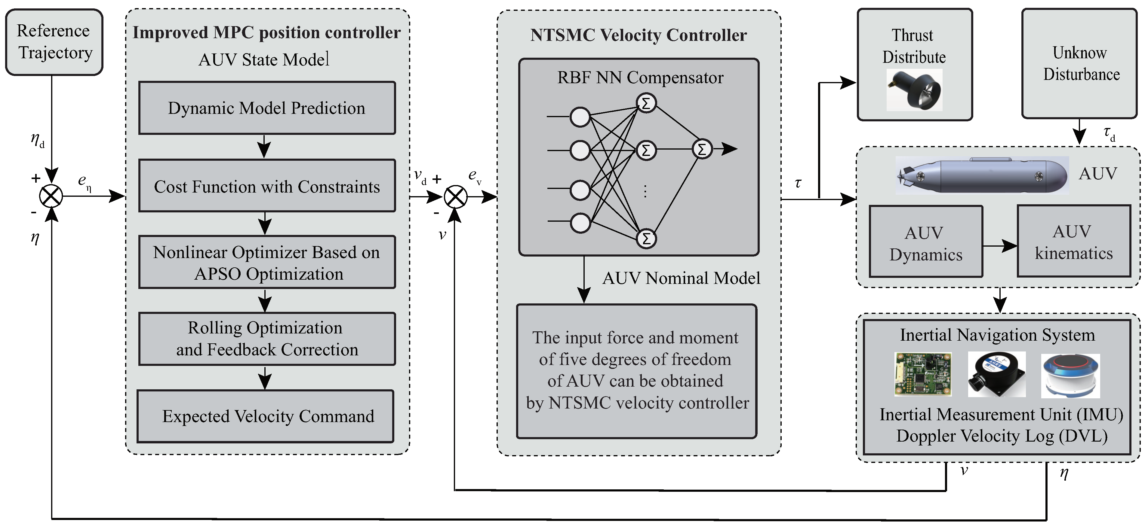
In this paper, an APSO-based MPC and NTSMC cascade control method is proposed and applied for the trajectory tracking control of an AUV. In the design of the controller, the actual constraints of the system are fully considered. When the APSO algorithm is applied to the MPC controller to solve the optimal speed instruction, it can overcome the problem of the standard MPC being unable to obtain the global optimal solution when applying the QP method to solve the problem with constraints. The NTSMC velocity controller allows the AUV to follow the expected optimal velocity commands. The adaptive RBF-NN compensator is designed to compensate for the modeling error of the AUV and the disturbance of external sea conditions to enhance the control accuracy and robustness of the system. The controller recalculates the best input at the next moment based on the system error within each sampling time of the system. The asymptotic stability of the controller is proven using a Lyapunov function with terminal constraints. Finally, a simulation model of AUV trajectory tracking control is built using MATLAB/Simulink. The simulation process includes setting two different expected trajectory cases, each of which includes settings without disturbance, with random disturbance, and with wave and/or current disturbance to verify the effectiveness and robustness of the proposed controller.
The main contents of this paper are as follows: Section 2 gives the kinematics and dynamics models of the fully actuated AUV, as well as the layout and rationality verification of the thrusters. Section 3 introduces the description of the trajectory tracking control problem and the design of the controller and analyzes the stability of the proposed controller. Section 4 gives the simulation results with different external disturbances. Section 5 provides some conclusive comments.

2. Modeling of the AUV System

AUV system modeling includes physical model design, kinematics modeling, dynamics modeling, and thrust distribution setting. The physical model design determines the basic physical parameters of the AUV and the layout of thrusters. The kinematics model of the AUV describes the relationship between its position, attitude, and velocity. The dynamic model describes the relationship between the acceleration and the force of the AUV in the process of motion.

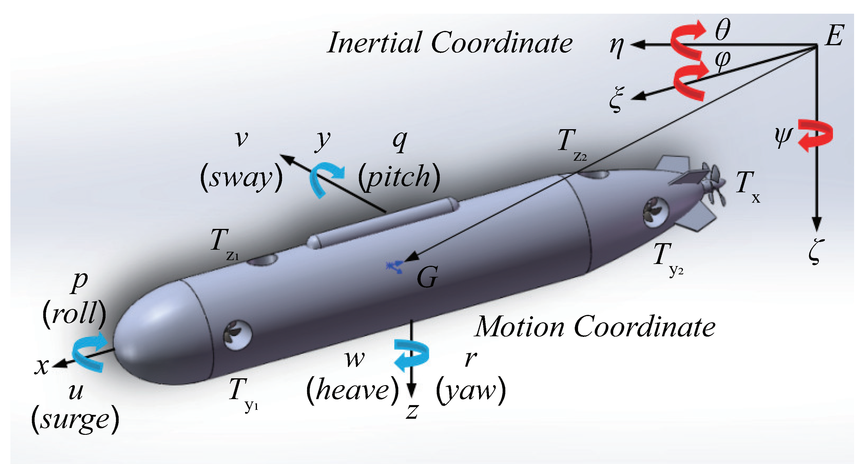
2.1. Frames of Reference

Figure 1 shows the fully actuated AUV design based on SOLIDWORKS proposed in this paper.
Remark 1. 
Generally, under the action of the restoring force and the moment of the AUV, the rolling motion of the AUV is considered to be self-stable, so the roll angle φ and roll angular velocity p of the rolling degrees of freedom are both 0. Similarly, pitch angular θ is bounded and satisfies π / 2 θ π / 2 [31].
Remark 2. 
The approximate solution method for the main inertial and viscous hydrodynamic coefficients of the fully actuated AUV proposed in this paper is based on the CFD simulation method in [34] and includes the simulation of uniform translational motion, uniform rotational motion, accelerated translational motion, and accelerated rotational motion.
Assumptions
1.
The AUV is treated as a rigid body with constant mass, and its gravity is assumed to be approximately equal to its buoyancy.
2.
The streamlined structure of the AUV is approximately symmetrical in the horizontal and vertical planes, and its hydrodynamic coefficient does not change with changes in the environment.
3.
The origin of the horizontal and vertical thrusters is coplanar with the center of gravity of the AUV, resulting in no corresponding moment disturbance.
The position and attitude information η = [ x , y , z , θ , ψ ] T of the AUV is defined in the inertial coordinate system E [36] corresponding to the information of five freedoms of motion: surge, sway, heave, pitch, and yaw.
The velocity information v = [ u , v , w , q , r ] T of the AUV is defined in the body coordinate system G corresponding to the information of the above five freedoms of motion. Here, E and G are both right-handed Cartesian coordinates.
Remark 3. 
The origin definition of G ( x G , y G , z G ) coincides with the center of gravity of the AUV proposed in this paper. The buoyancy force of the AUV is defined as B, and the center of buoyancy coordinate is ( x B , y B , z B ) .

2.2. Kinematics and Dynamics

The kinematic model of the fully actuated AUV can be defined:
η ˙ = J ( η ) v
where J ( η ) is defined as the transition matrix between the coordinates of E and G:
J ( η ) = cos ψ cos θ sin ψ sin θ cos ψ 0 0 sin ψ cos θ cos ψ sin θ sin ψ 0 0 sin θ 0 cos θ 0 0 0 0 0 1 0 0 0 0 0 1 / cos θ
The general dynamics model of the underwater vehicle proposed by Fossen [33] is also applicable to the fully actuated AUV proposed in this paper and can be expressed in the following form:
M v ˙ + C ( v ) v + D ( v ) v + g ( η ) + τ d = τ
where M = d i a g ( m X u ˙ , m Y v ˙ , m Z w ˙ , I y M q ˙ , I z N r ˙ ) is defined as the inertia matrix, with m the mass of the AUV and I x , I y , and I z the inertia tensors of AUV. The values in this paper can be obtained from the SOLIDWORKS structural model of the designed AUV. Here, X u ˙ , Y v ˙ , Z w ˙ , M q ˙ , and N r ˙ are the main inertial hydrodynamic coefficient caused by the AUV performing accelerated motion underwater [37], where C ( v ) = C RB ( v ) + C A ( v ) . Because of the Earth’s rotation, an AUV naturally experiences Coriolis and centripetal effects when moving underwater.
Here, C RB ( v ) and C A ( v ) are the Coriolis and centripetal force matrices caused by the above rigid body inertial mass matrix and the additional mass matrix, respectively.
Specifically,
C RB ( v ) = 0 0 0 m w m v 0 0 0 0 m u 0 0 0 m u 0 m v 0 m u 0 0 m v m u 0 0 0
C A ( v ) = 0 0 0 Z w ˙ w Y v ˙ v 0 0 0 0 X u ˙ u 0 0 0 X u ˙ u 0 Z w ˙ w 0 X u ˙ u 0 0 Y v ˙ v X u ˙ u 0 0 0
where D ( v ) = d i a g ( X u X u u u , Y v Y v v v , Z w Z w w w , K p K p p p , M q M q q q , N r N r r r ) is defined as the viscous damping matrix.
X u , Y v , Z w , M q , N r , X u u , Y v v , Z w w , M q q , and N r r are estimable linear and nonlinear viscous hydrodynamic coefficients, respectively.
Here, g ( η ) is the restoring force matrix generated by the static force of the AUV in the underwater environment.
g ( η ) = 0 0 0 y B B cos θ z B B sin θ x B cos θ y B B sin θ
τ d = [ τ d u , τ d v , τ d w , τ d q , τ d r ] T is the the vector of external unknown ocean disturbance force and moment for each degree of freedom.
τ = [ τ u , τ v , τ w , τ q , τ r ] T is the vector of the thruster input force and moment for each degree of freedom.

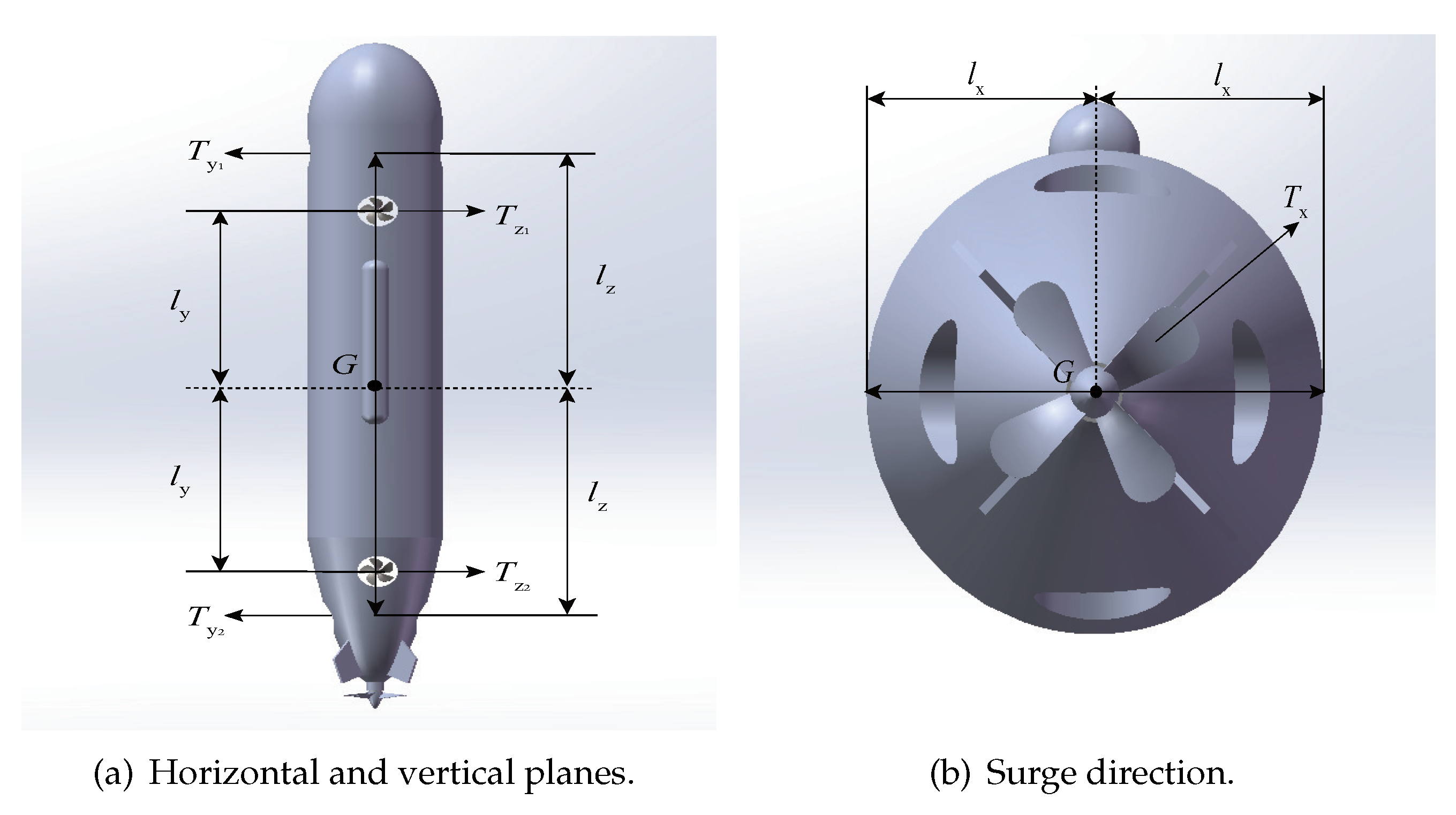
2.3. Thruster Layout and Rationality Verification

The thruster arrangement of the fully actuated AUV proposed in this paper is shown in Figure 2, where T x is the main thruster arranged in the surge direction, T y 1 and T y 2 are the two thrusters arranged in the sway direction, and T z 1 and T z 2 are the two thrusters arranged in the heave direction. The values l x , l y , and l z are the moment arms in the corresponding direction.
In order to complete the motion control task, τ = [ τ u , τ v , τ w , τ q , τ r ] T should be assigned to the appropriate thrusters. Based on the thruster arrangement in Figure 2, the thrust distribution matrix equation can be easily obtained in the following form:
τ = τ u τ v τ w τ q τ r = 1 0 0 0 0 0 1 1 0 0 0 0 0 1 1 0 0 0 l z l z 0 l y l y 0 0 T x T y 1 T y 2 T z 1 T z 2
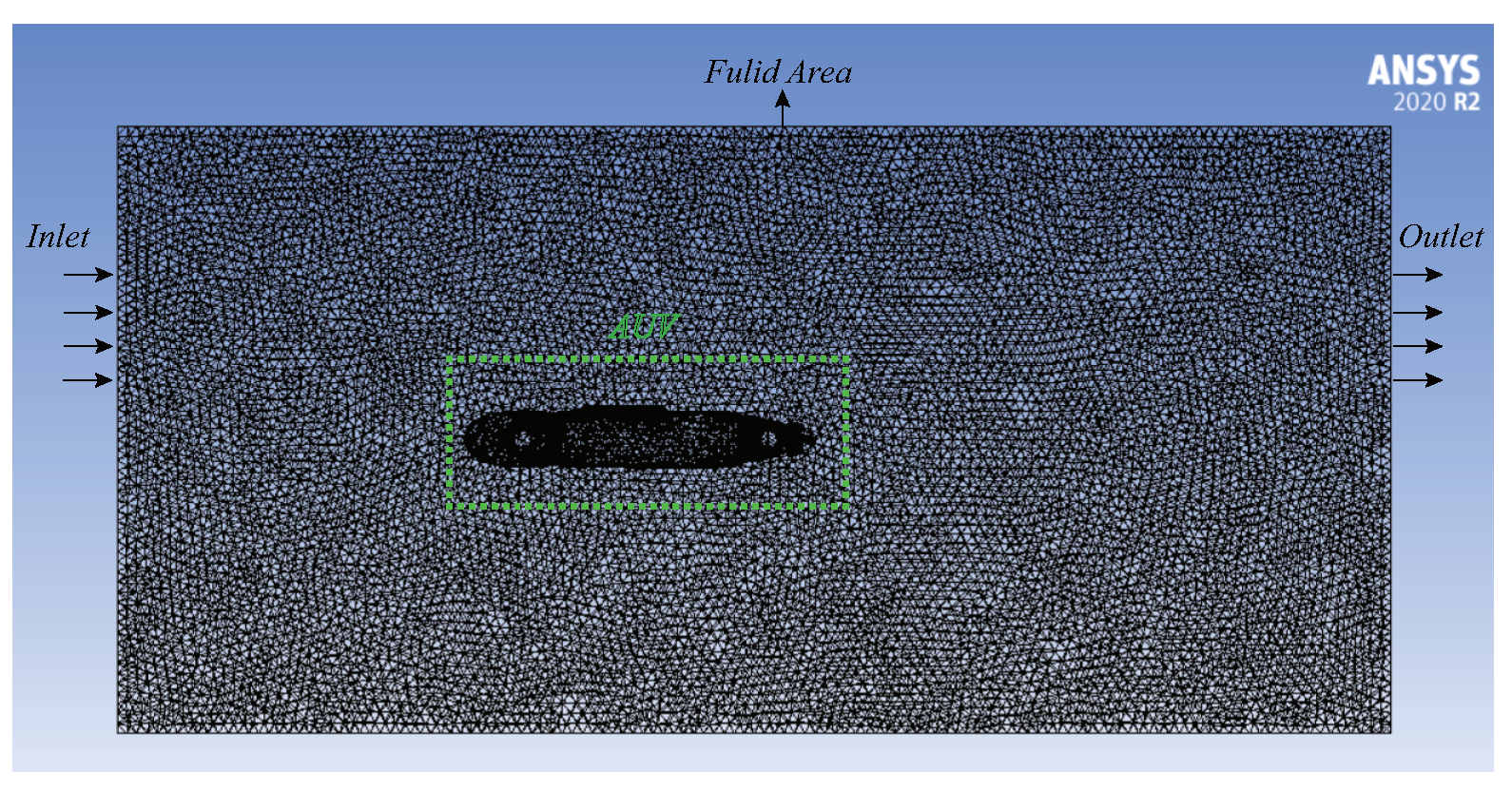
To reasonably choose the type of thruster, this paper used computational fluid dynamics (CFD) software ANSYS-FLUENT to simulate surge, sway, and heave motions of the AUV at different velocities to solve for the maximum drag value. The mesh part of the AUV in the CFD software FLUENT is shown in Figure 3.
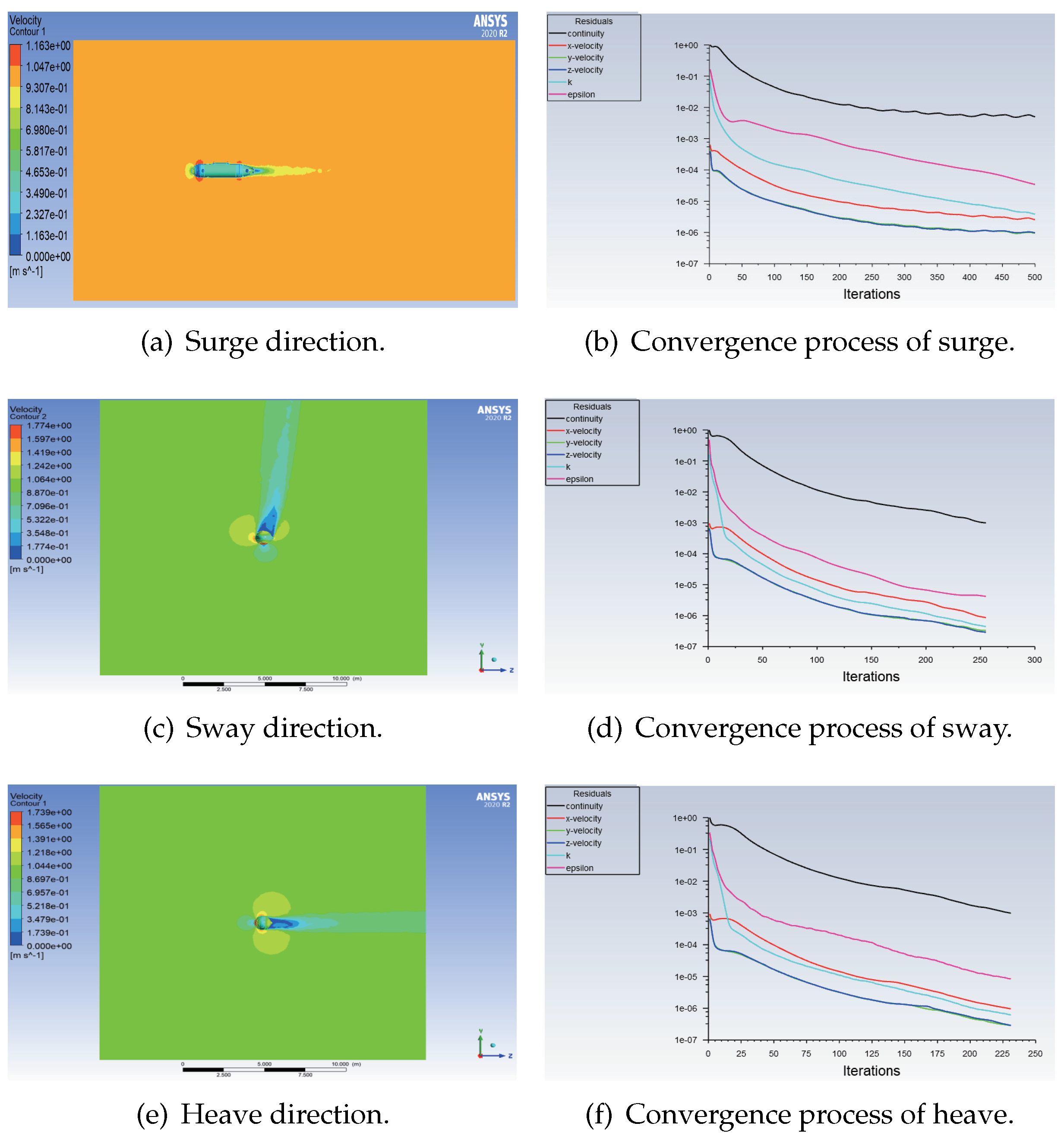
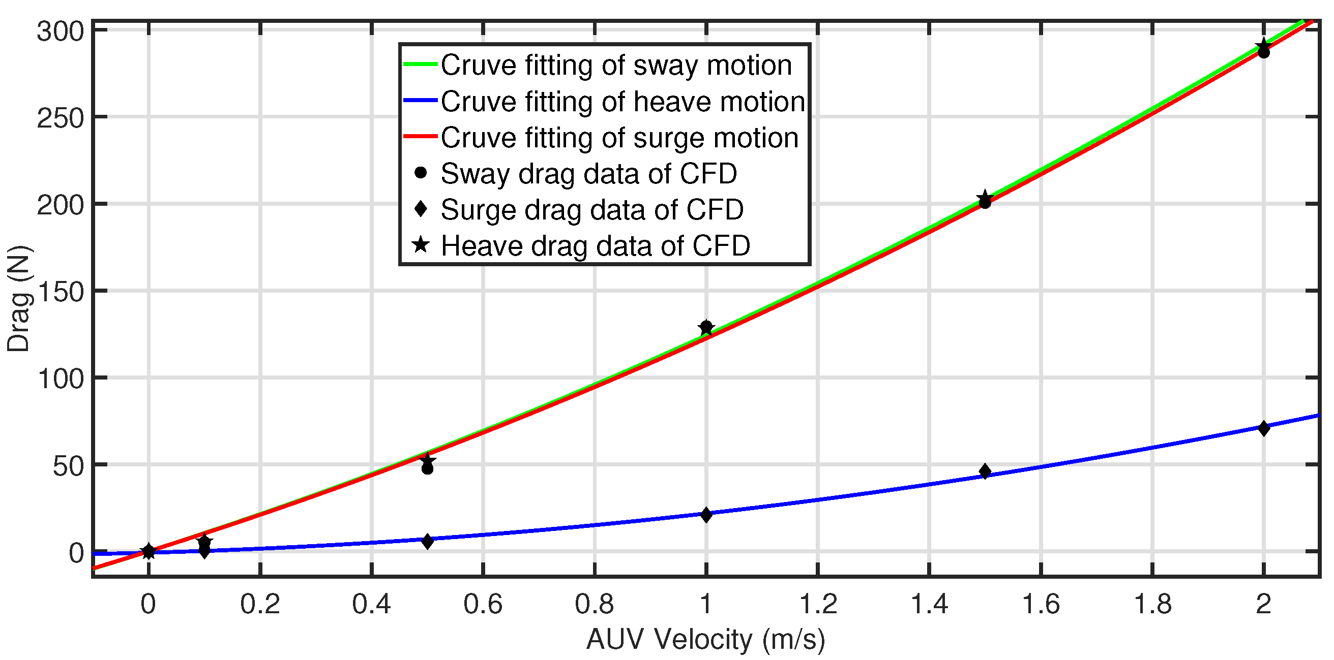
Figure 4 shows the relevant process and data of the CFD simulation. It can be seen from the figure that when the velocity is about 3 knots, the maximum drag in the surge, sway, and heave directions is about 46 N, 180 N, and 180 N, respectively.
The design velocity of the fully actuated AUV proposed in this paper is 2 knots. Based on the CFD simulation data, the velocity values of the AUV’s surge, sway, and heave freedom and the corresponding drag values are respectively fitted. The fitting results are shown in Figure 5. Based on the fitting results, an S100-CR-IC electric thruster is selected for the AUV.
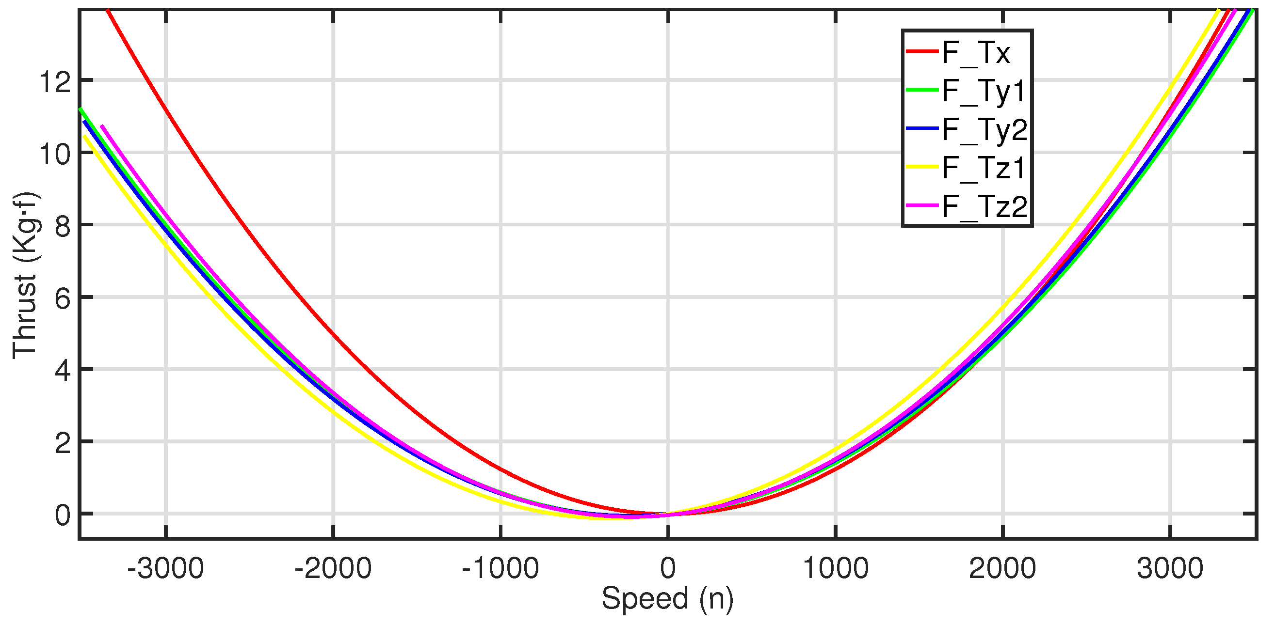
As can be can clearly seen from Figure 6, the maximum forward thrust of a single thruster is 13.5 kg · f , which is about 135 N. The maximum reverse thrust is about 9 kg · f , or about 90 N. Based on the above data, the arrangement of thrusters in this paper is reasonable.

3. Design of the Controller

This paper focuses on the trajectory tracking control of an AUV with external disturbances. The main control objective is to ensure that the position and velocity of the AUV remain consistent with time. The closed-loop control system consists of an MPC position controller optimized based on the APSO algorithm and a sliding mode velocity controller. The former uses the system output feedback to design the expected velocity to ensure convergence of the AUV position tracking error. The latter achieves gradual convergence of the AUV drive velocity to the expected command, i.e., it ensures convergence of the AUV velocity tracking error. The optimal control solution can be found more effectively by considering the corresponding constraints when designing each controller. The block diagram of the cascade control strategy based on the RBF-NN compensator proposed in this paper is shown in Figure 7.

3.1. Design of MPC-APSO Controller

The trajectories are assumed to be pre-given functions of time that satisfy smooth, bounded, and second-order differentiable functions. We set the expected trajectory to be tracked by the fully actuated AUV as follows:
Y d = [ x d , y d , z d , θ d , ψ d ] T
The MPC-APSO controller is the guidance controller of the AUV trajectory tracking control; that is, it is the kinematics controller. We set the sampling time T s of the MPC rolling optimization. The discrete motion model of the AUV can be defined as follows:
η ( k + 1 ) = η ( k ) + J ( k ) v ( k ) T s
The velocity increment of an AUV is defined as the input of the guidance controller to ensure the stability of its motion. Based on the MPC principle, the state model of an AUV can be defined as follows:
X ( k + 1 ) = [ η ( k + 1 ) , v ( k ) ] T
Therefore, the input of the system is defined as:
Δ v ( k ) = v ( k ) v ( k 1 )
By combining Equations (9)–(11), the state space model can be rewritten in the following form:
X ( k + 1 ) = η ( k + 1 ) = η ( k ) + J ( k ) v ( k ) T s + J ( k ) v ( k 1 ) T s J ( k ) v ( k 1 ) T s v ( k ) + v ( k 1 ) v ( k 1 ) = η ( k ) + J ( k ) v ( k 1 ) T s v ( k 1 ) + J ( k ) v ( k ) T s + J ( k ) v ( k 1 ) T s v ( k ) v ( k 1 ) = I 5 J ( k ) T s 0 5 × 5 I 5 η ( k ) v ( k 1 ) + J ( k ) T s I 5 v ( k ) v ( k 1 )
where Y ( k ) is the output. By introducing the two matrices Γ A ( k ) and Γ B ( k ) , we can get the following form:
X ( k + 1 ) = Γ A ( k ) X ( k ) + Γ B ( k ) Δ v ( k ) ,   Y ( k ) = Λ X ( k )
with
Γ A ( k ) = I 5 J ( k ) T s 0 5 × 5 I 5 ,   Γ B ( k ) = J ( k ) T s I 5 ,   Λ = I 5 0 5 × 5
where I 5 is a 5 × 5 identity matrix, and 0 5 × 5 is a 5 × 5 zero matrix.
Definitions N p and N c are the prediction horizon and control horizon, respectively, and satisfy N c N p . The predicted sequence of the state and the output can be expressed in the following form:
X N p = X ( k + 1 | k ) X ( k + 2 | k ) X ( k + N p | k ) , Y N p = Y ( k + 1 | k ) Y ( k + 2 | k ) Y ( k + N p | k )
The control sequence of the velocity increment as an input to the MPC controller is as follows:
Δ v ( k ) = Δ v ( k + 1 | k ) Δ v ( k + 2 | k ) Δ v ( k + N p 1 | k )
Based on MPC control theory, the predictive control system model of the AUV can be rewritten as follows:
X ¯ ( k + 1 ) = Γ ¯ A ( k ) X ( k ) + Γ ¯ B ( k ) Δ v ( k )
Here,
Γ ¯ A ( k ) = [ Γ A ( k ) , Γ A ( k ) 2 , , Γ A ( k ) N p ] T
Γ ¯ B ( k ) = Γ B ( k ) 0 0 Γ A ( k ) Γ B ( k ) Γ B ( k ) 0 Γ A ( k ) N p 1 Γ B ( k ) Γ A ( k ) N p 2 Γ B ( k ) Γ B ( k )
The advantage of MPC is that it can solve practical problems with constraints. Here, the constraints of the control input and the AUV state are given as follows:
Δ v m i n Δ v ( k ) Δ v m a x
X m i n X ( k ) X m a x
Based on the current state and predicted future state, the cost function of MPC rolling optimization is:
H ( t ) = 0 T [ Y ( t ) Y d ( t ) Γ y 2 + Δ v ( t ) Γ Δ v 2 ]
where
y Γ y 2 = y T Γ y y , Δ v Γ Δ v 2 = Δ v T Γ Δ v Δ v
The symmetrical positive definite weight matrices Γ y and Γ Δ v are introduced. The discretized form of E ( t ) is as follows:
H ( k ) = i = 1 N p [ Y ( k + i | k ) Y d ( k + i | k ) Γ y 2 + Δ v ( k + i 1 | k ) Γ Δ v 2 ]
Based on Equation (13), Equation (24) can be rewritten as follows:
H ( k ) = i = 1 N p [ X ( k + i | k ) X d ( k + i | k ) Γ x 2 + Δ v ( k + i 1 | k ) Γ Δ v 2 ]
where
X ( k + i ) = Λ Y ( k + i ) ,   Γ x = Λ Γ y Λ
The pseudo inverse matrix of Λ represents Λ . Based on Equation (17), a simplification of Equation (25) can be written as:
H ( k ) = X ¯ ( k ) X ¯ d ( k ) Γ ¯ x 2 + Δ v ( k ) Γ ¯ Δ v 2
where Γ ¯ x = d i a g ( Γ x , Γ x , Γ x , Γ x , Γ x ) , Γ ¯ Δ v = d i a g ( Γ Δ v , Γ Δ v , Γ Δ v , Γ Δ v , Γ Δ v ) .
It can be clearly concluded from Equation (27) that the only independent variable of E ( k ) is Δ v ( k ) , so the problem of obtaining the MPC optimal control sequence of the AUV is equivalent to the control input sequence of solving the minimum value of E ( k ) with Equations (20) and (21) with constraints. The expression is as follows:
Δ v * ( k ) = argmin Δ v ( k ) E ( k )

3.2. APSO for Solving the Cost Function

In this part, the APSO method is introduced in place of the QP method to obtain the minimum value of E ( k ) . The adaptive inertia weight is introduced to improve the optimization effect and convergence velocity of the traditional PSO algorithm. The prediction input Δ v ( k ) is used as the optimization variable. In the MPC process, the dimensionality D of each particle in the particle swarm is the control horizon N c .
(1)
Initialize the particle swarm.
Set the population size N p s and constrict the position of each particle in the search area. The position of the ith particle is expressed as x i = ( x i 1 , x i 2 , , x i D ) , i = ( 1 , 2 , , N p s ) . The fitness function for MPC is the objective function given in Equation (24). The best position experienced by the ith particle, that is, the position with the smallest fitness function value, is expressed as p i = ( p i 1 , p i 2 , , p i D ) , i = ( 1 , 2 , , N p s ) . The best position experienced among all particles in the population is expressed as p g = ( p g 1 , p g 2 , , p g D ) , g = ( 1 , 2 , , N p s ) .
(2)
Adaptive inertia weight.
To effectively control the flight velocity of particles and make the algorithm achieve an effective balance between local search and global search, we constructed the PSO model with the introduction of an adaptive inertia weight Υ . This adjustment method can ensure the convergence of the PSO algorithm by appropriately selecting parameters and can remove the boundary restriction on velocity. In the application of solving the optimal value, a large inertia weight should be applied at the beginning of the APSO algorithm to increase the searchability of the algorithm and avoid obtaining a local optimal solution. As the algorithm progresses, the inertia weight should be gradually reduced to enhance the local searchability of the algorithm and accelerate the convergence of the algorithm to obtain the global optimal solution. Adaptive inertia weight Υ is defined as:
Υ i d k = Υ m i n + ( Υ m a x Υ m i n ) E ( x i d k ) E m i n k E a v k E m i n k ,   E ( x i d k ) E m i n k Υ m a x ,   E ( x i d k ) > E m i n k
The particle velocity update function is
v i d k + 1 = Υ i d k v i d k + c 1 r 1 ( p i d k x i d k ) + c 2 r 2 ( p g d k x g d k )
where c 1 and c 2 are learning factors, which are normal numbers; and r 1 and r 2 are random numbers between 0 and 1. The velocity of the ith particle is expressed as v i = ( v i 1 , v i 2 , , v i D ) , i = ( 1 , 2 , , N p s ) . The particle position update function is as follows:
x i d k + 1 = x i d k + v i d k + 1
(3)
Operation process of APSO algorithm.
We use the fitness function given in Equation (24) to calculate the historical optimal value of each individual particle and the historical optimal value of the entire particle range (global). We update the current state of each particle using the position and velocity update functions in Equations (30) and (31). We repeat the above calculation process.
The flow of the particle swarm optimization algorithm with the adaptive compression factor is shown in Algorithm 1.
Algorithm 1 Pseudocode of particle swarm optimization algorithm with adaptive inertia weight.
  • Start of Algorithm;
  • Input: Maximum number of iterations: N m a x ; current iteration number: N c u r r e n t ; number of particles: N p s ;
  • APSO initialization: Initialize the particle swarm (position and velocity). Equation (22) is used to evaluate the initial fitness value of each particle;
  • while ( N c u r r e n t N m a x ) ;
  • Step 1: Rank the fitness values and find the current best X b e s t N c u r r e n t and worst individual X w o r s t N c u r r e n t ;
  • Step 2: The adaptive inertia weight Υ of Equation (29) is introduced into the position update equation of the algorithm;
  • Step 3: Use Equation (30) to update the velocity of the particles;
  • Step 4: Use Equation (31) to update the position of the particles;
  • Step 5: Get the current new position of all particles;
  • Step 6: If the new best particle location is better than the previous one, update it;
  • N c u r r e n t = N c u r r e n t + 1 ;
  • end while.
  • Return Step 1.
  • Stop iterating when the maximum number of iterations is reached or the optimal solution is converged on.
  • Output: X b e s t N m a x .
  • End of Algorithm.
We set a maximum number of iterations. The output optimal solution X b e s t N m a x is the optimal control sequence Δ v * ( k ) of MPC. We feedback the first component Δ v * ( k + 1 | k ) of the optimal control sequence Δ v * ( k ) to the control system. The optimal velocity command transmitted to the NTSMC velocity controller is:
v d ( k ) = v ( k ) + Δ v * ( k + 1 | k )

3.3. Stability Analysis of MPC-APSO Controller

In this part, we introduce terminal constraints to analyze the stability of the MPC-APSO controller.
Lemma 1. 
By using the traditional Lyapunov stability proof method in control theory, which finds a positive definite Lyapunov function whose inverse is negative definite, the stability of the controller is proved.
Proof. 
At current moment k, the optimal velocity increment sequence obtained by MPC-APSO can be defined as:
Δ v * ( k ) = Δ v * ( k | k ) Δ v * ( k + 1 | k ) Δ v * ( k + N p 1 | k )
After the terminal constraint is introduced, the optimal AUV state sequence and output sequence can be defined as:
X k * ( k + 1 | k ) , X k * ( k + 2 | k ) , , X k * ( k + N p 1 | k ) , 0 Y k * ( k + 1 | k ) , Y k * ( k + 2 | k ) , , Y k * ( k + N p 1 | k ) , 0
The optimal cost function can be expressed as follows:
H * ( k ) = i = 0 N p 1 [ X * ( k + i | k ) X d ( k + i | k ) Γ y 2 + Δ v * ( k + i | k ) Γ Δ v 2 ]
For the MPC-APSO controller, H * ( k ) is defined as Lyapunov function H m * ( k ) according to the Lyapunov stability theorem.
H m * ( k ) = i = 0 N p 1 [ X * ( k + i | k ) X d ( k + i | k ) Γ y 2 + Δ v * ( k + i | k ) Γ Δ v 2 ]
Clearly, Equation (36) satisfies H m * ( 0 ) = 0 with k = 0 and H m * ( k ) > 0 with arbitrary k 0 .
In Equations (33) and (34), X * ( k | k ) = X ( k ) and Δ v * ( k | k ) = Δ v ( k ) . By combining these with Equation (13), we can easily obtain:
X ( k + 1 ) = Γ A ( k ) X ( k ) + Γ B ( k ) Δ v * ( k | k ) = X * ( k + 1 )
When time k + 1 is reached, this control sequence of MPC-APSO is in the following form:
Δ v ( k + 1 ) = Δ v * ( k + 1 | k ) Δ v ( k + 2 | k ) Δ v ( k + N p 1 | k ) 0
With the conditions of satisfying terminal constraints and system constraints, the status sequence of the AUV is:
X ( k + i + 1 | k + 1 ) = X * ( k + i + 1 | k ) , i = 0 , , N p 1 0 , i = N p
By substituting Equations (38) and (39) into Equation (25), we obtain
H ( k + 1 ) = i = 0 N p 1 [ X ( k + i + 1 | k + 1 ) X d ( k + i + 1 | k + 1 ) Γ x 2 + Δ v ( k + i + 1 | k + 1 ) Γ Δ v 2 ] = i = 0 N p 2 [ X * ( k + i + 1 | k ) X d ( k + i + 1 | k ) Γ x 2 + Δ v * ( k + i + 1 | k ) Γ Δ v 2 ] = i = 1 N p 1 [ X * ( k + i | k ) X d ( k + i | k ) Γ x 2 + Δ v * ( k + i | k ) Γ Δ v 2 ] = i = 0 N p 1 [ X * ( k + i | k ) X d ( k + i | k ) Γ x 2 + Δ v * ( k + i | k ) Γ Δ v 2 ] X * ( k | k ) X d ( k | k ) Γ x 2 Δ v * ( k | k ) Γ Δ v 2 = H * ( k ) X * ( k | k ) X d ( k | k ) Γ x 2 Δ v * ( k | k ) Γ Δ v 2
Obviously,
H * ( k + 1 ) H ( k + 1 ) = H * ( k ) X * ( k | k ) X d ( k | k ) Γ x 2 Δ v * ( k | k ) Γ Δ v 2
H m * ( k + 1 ) H m * ( k )
Here, the contents of Equation (36) conform to Lemma 1. Thus, Equation (17) is nominally stable. □

3.4. Design of NN-NTSMC Velocity Controller

In this part, the NTSMC velocity controller is designed to enhance the control accuracy and robustness of the AUV control system. The task of the controller is to determine the forces and moments that drive the AUV based on the input velocity errors. At the same time, the RBF-NN compensator is designed to compensate for the dynamic modeling error of the AUV and the influence of external interference on the control system.
Obviously, it is difficult to obtain the complete model information of the AUV in practice. Equation (3) is only the nominal model of the AUV, and when the AUV works in an underwater environment, the real-time disturbances of the external environment to the AUV are also unknown. Therefore, the dynamic modeling error of the AUV can be expressed as the following unknown function:
Θ ( η , v , v ˙ ) = Δ M v ˙ + Δ C v + Δ D v + Δ g ( η ) + τ d
Here, Δ M , Δ C , Δ D , and Δ g are the error matrices corresponding to the nominal model and the actual model of the dynamics, respectively. Therefore, Equation (3) should be rewritten as follows:
M v ˙ + C ( v ) v + D ( v ) v + g ( η ) + Θ ( η , v , v ˙ ) = τ
Remark 4. 
An RBF neural network can approximate any smooth unknown function Θ ( · ) in the following form [38]:
Θ ( · ) = i = 1 n ω i * h i ( · ) + ε ( · )
where n is the number of neurons in the hidden layer, and ε ( · ) is the steady-state error of the NN. The value ω i * is the optimal connection weight between the ith neuron in the hidden layer and the output layer, which is defined as:
i = 1 n ω i * = argmin [ i = 1 n ω i * h i ( · ) f ( · ) ]
Here, h i ( · ) is the activation function of the neurons in the hidden layer. This paper selects the radial basis function–Gaussian function, which is defined as follows:
h i ( ϕ ( k 1 ) ) = e h ( · ) μ i 2 2 σ i 2
where μ i is the center vector of the hidden layer neuron, and σ i is the width of the ith neuron in the hidden layer. The function h ( · ) μ i is the euclidean distance between the input matrix and the center of the radial basis.
In this paper, a three-layer feed-forward RBF NN is used to construct the unknown item Θ ( η , v , v ˙ ) in Equation (44). The proposed RBF-NN compensator uses k-means to determine the cluster center and width, and it uses the gradient-descent-based optimization method to update the network weight. The actual estimate of the unknown item is as follows:
Θ ^ ( η , v , v ˙ ) = i = 1 n ω ^ i h ^ i ( · ) + ε ( · )
The difference between the optimal expected velocity of the system obtained by MPC-APSO and the actual velocity of the AUV is used as the input to the NTSMC dynamics controller and is defined as follows:
e v = v d v = [ e u , e v , e w , e q , e r ] T   e ˙ v = v ˙ d v ˙ = [ e ˙ u , e ˙ v , e ˙ w , e ˙ q , e ˙ r ] T
Here, v d = [ v d u , v d v , v d w , v d q , v d r ] T . The non-singular terminal sliding mode surface function is designed as follows:
s = e ˙ v + 1 δ e v α / β
Here, δ > 0 , α , and β are odd numbers and satisfy α > β > 0 . A hyperbolic tangent function is used instead of a sign function to reduce the jump at 0, and its exponential approach law is used:
s ˙ = e ¨ v + α δ β e v ( α β β ) e ˙ v = tanh ( s γ ) = [ t a n h ( s γ ) u , t a n h ( s γ ) v , t a n h ( s γ ) w , t a n h ( s γ ) q , t a n h ( s γ ) r ] T = ( v ¨ d v ¨ ) + α δ β ( v d v ) ( α β β ) ( v ˙ d v ˙ )
Here, γ > 0 denotes the velocity at which the moving point of the system approaches the switching surface s = 0 . Obviously, Equation (51) can be transformed into the following form:
v ˙ = v ˙ d ( v v d ) ( α β β ) α δ β [ v ¨ v ¨ d tanh ( s γ ) ]
According to Equations (44) and (48), we can obtain:
v ˙ = M 1 [ τ C ( v ) v D ( v ) v g ( η ) Θ ^ ( η , v , v ˙ ) ]
According to Equations (3) to (5), by combining Equations (52) and (53), the amount of control for each degree of freedom of the AUV can be obtained:
τ x = ( m X u ˙ ) ( v ˙ d u ( u v d u ) ( α β β ) δ β α [ u ¨ u ¨ d t a n h ( s γ ) ] ) + m ( w q v r ) Z w ˙ w q + Y v ˙ v r + ( X u ˙ u + X u u u ) u + Θ ^ ( η , v , v ˙ ) x
τ y = ( m Y v ˙ ) ( v ˙ d v ( v v d v ) ( α β β ) δ β α [ v ¨ v ¨ d t a n h ( s γ ) ] ) + u r ( m X u ˙ ) + ( Y v ˙ u + Y v v v ) v + Θ ^ ( η , v , v ˙ ) y
τ z = ( m Z w ˙ ) ( v ˙ d w ( w v d w ) ( α β β ) δ β α [ w ¨ w ¨ d t a n h ( s γ ) ] ) u q ( m X u ˙ ) + ( Z w ˙ w + Z w w w ) w + Θ ^ ( η , v , v ˙ ) z
τ θ = ( I y M q ˙ ) ( v ˙ d q ( q v d q ) ( α β β ) δ β α [ q ¨ q ¨ d t a n h ( s γ ) ] ) + m u ( w v ) + w u ( Z w ˙ X u ˙ ) + ( M q ˙ q + M q q q ) q z B B sin θ x B cos θ + Θ ^ ( η , v , v ˙ ) θ
τ ψ = ( I z N r ˙ ) ( v ˙ d r ( r v d r ) ( α β β ) δ β α [ r ¨ r ¨ d t a n h ( s γ ) ] ) + u v ( X u ˙ Y v ˙ ) + ( N r ˙ r + N r r r ) r + y B B sin θ + Θ ^ ( η , v , v ˙ ) ψ

3.5. Stability Analysis of RBF-NTSMC Controller

For the NTSMC velocity controller, the Lyapunov function H s * ( k ) is defined as follows:
H s * ( k ) = 1 2 s 2
H ˙ s * ( k ) = s ˙ s = s tanh ( s γ ) = s
It can be readily derived that L s * ( k ) > 0 and L ˙ s * ( k ) < 0 , and that this also satisfies Lemma 1. Thus, the system is stable at the equilibrium point s = 0 , satisfying the conditions of the Lyapunov function, and s eventually stabilizes the NTSMC surface.

4. Simulation Results

In this part, MATLAB/Simulink are used to verify the effectiveness of the proposed cascade controller (MPC-APSO-NTSMC) in AUV 3D trajectory tracking control. The simulation results are compared with the simulation results of the position and velocity double-closed-loop proportional differential (PD) controller (PD-PD) and the traditional MPC and linear SMC cascade controller (MPC-PSO-SMC).
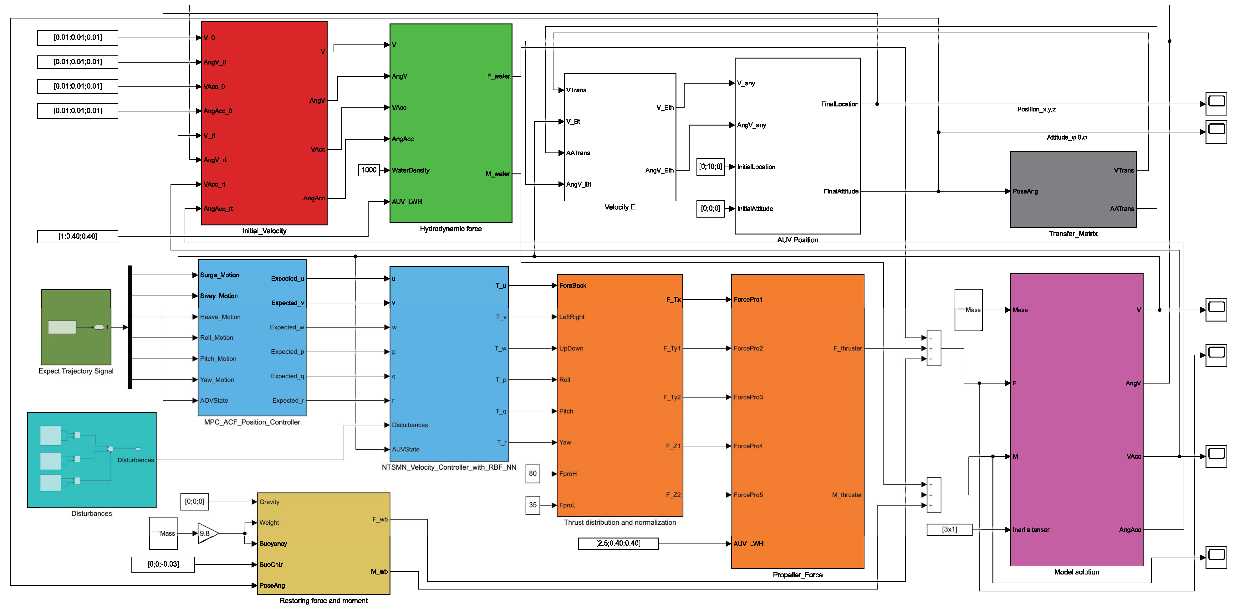
The simulation and verification process is divided into two trajectory tracking cases: spiral trajectory tracking and complex curve tracking. The Simulink simulation model is shown in Figure 8. The basic physics and main hydrodynamic coefficients of the AUV are shown in Table 1. The simulation parameters are shown in Table 2.
The random disturbance in the simulation is defined as follows:
r a n d u = 0.1 × rand ( 1 ) , ( m / s ) r a n d v = 0.1 × rand ( 1 ) , ( m / s ) r a n d w = 0.1 × rand ( 1 ) , ( m / s )
Here, rand(1) represents a random number between 0 and 1. The wave and current disturbance in the simulation is defined as follows:
w a v e u = 0.1 sin ( π / 8 · t ) + 0.1 , ( m / s ) w a v e v = 0.1 sin ( π / 8 · t ) + 0.1 , ( m / s ) w a c e w = 0.1 sin ( π / 8 · t ) + 0.1 , ( m / s )
Case 1: We set the initial position of the fully actuated AUV in the underwater simulation environment to be η ( 0 ) = [ 0 , 10 , 0 , 0 , 0 ] T , and the function of the spiral trajectory with time is defined as follows:
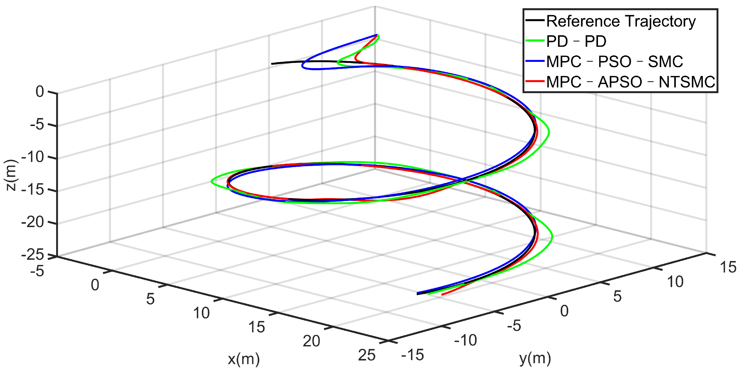
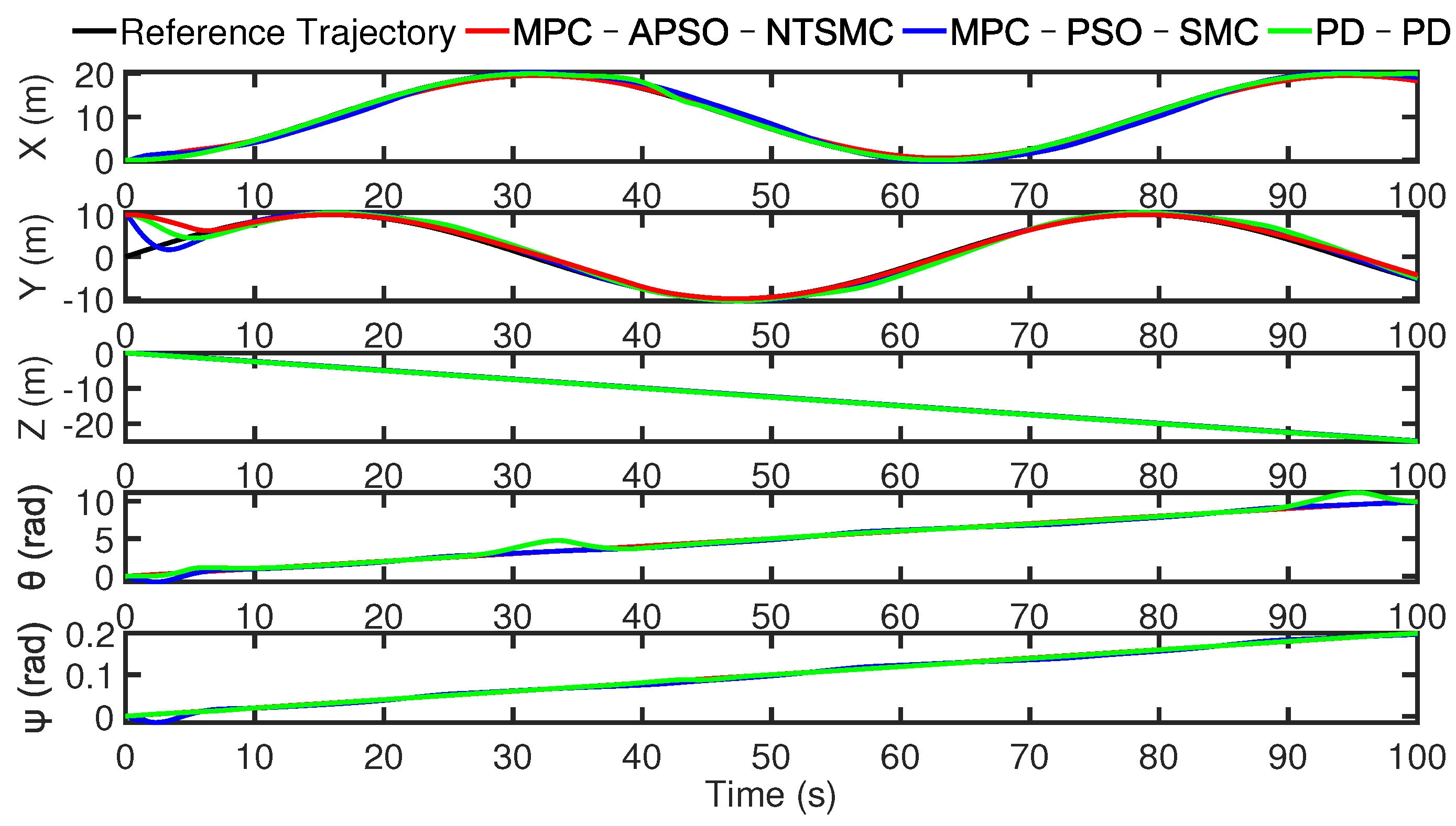
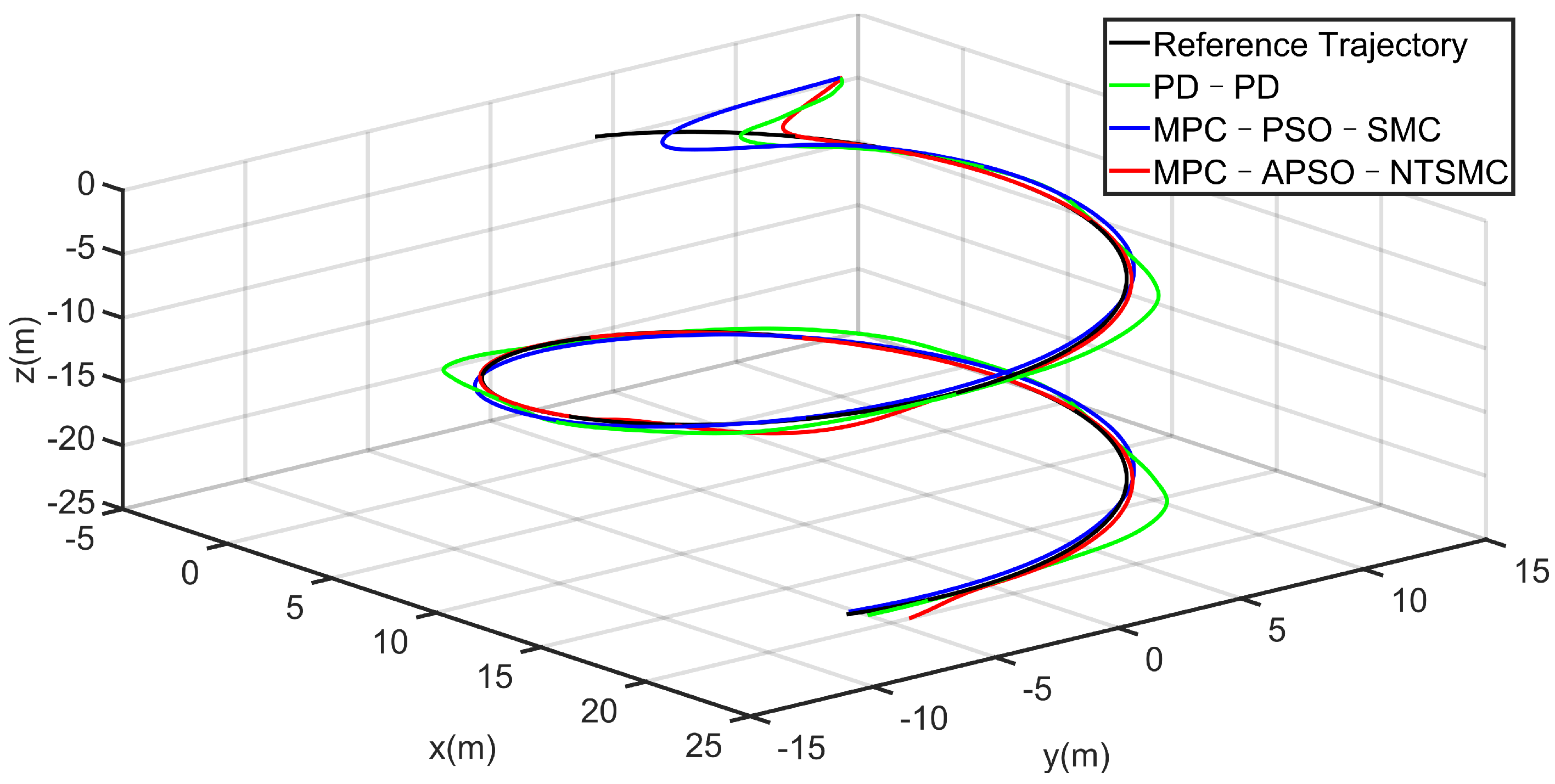
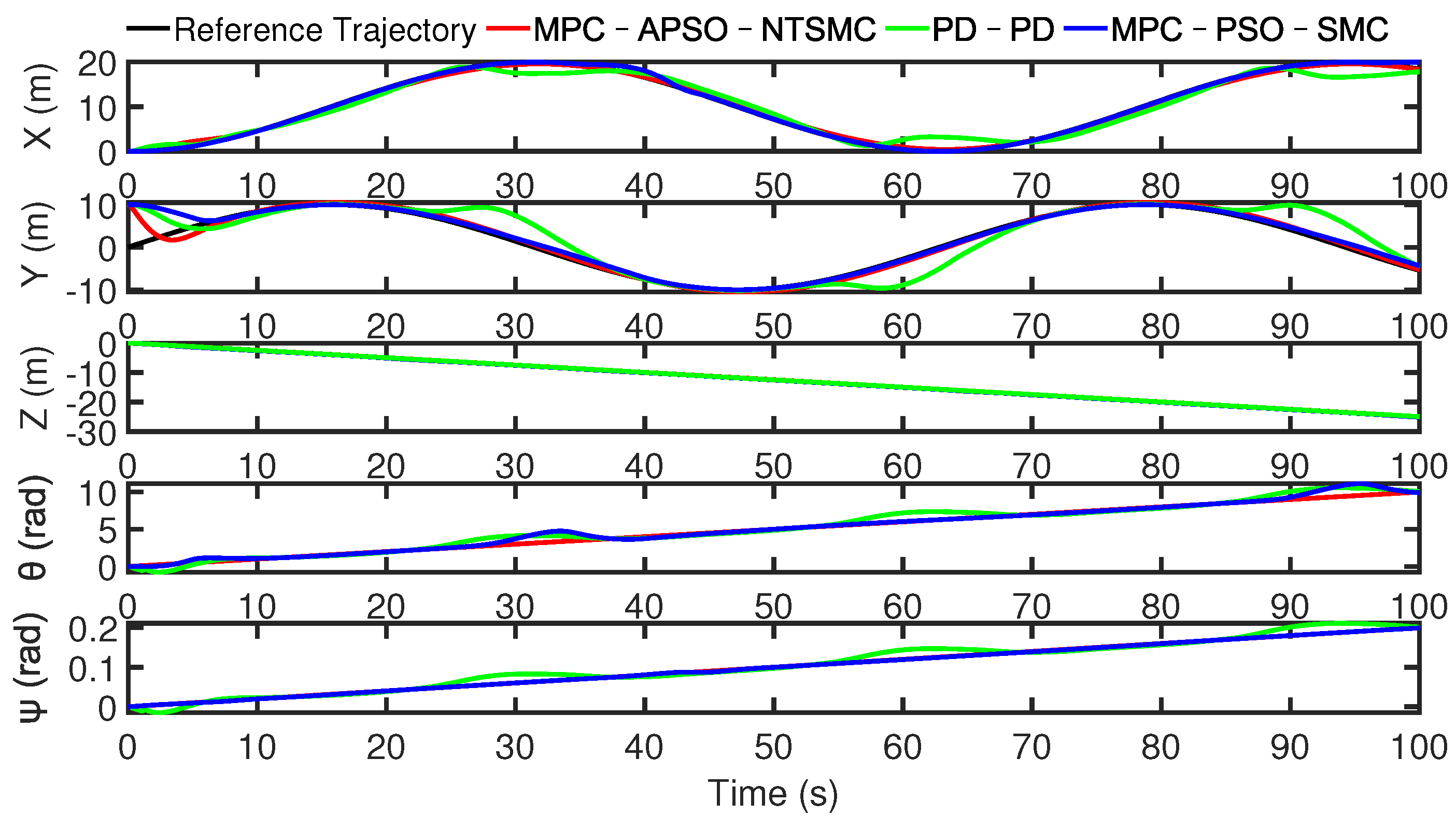
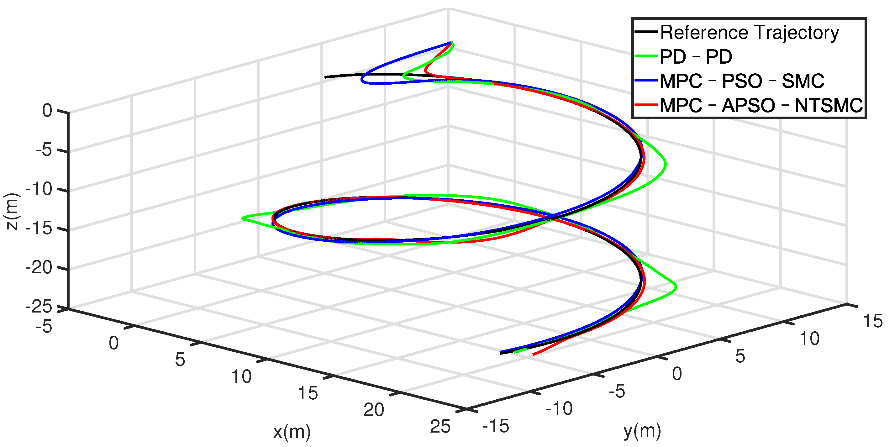
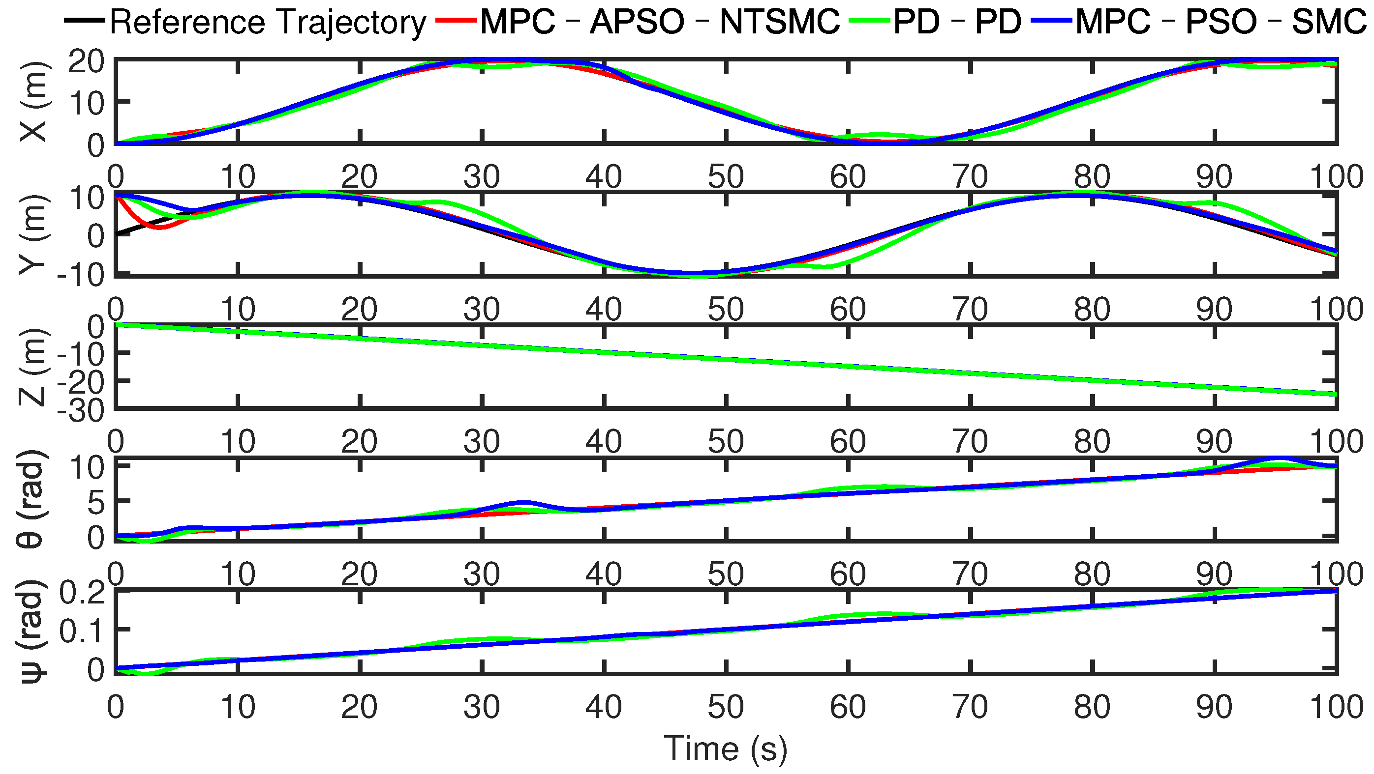
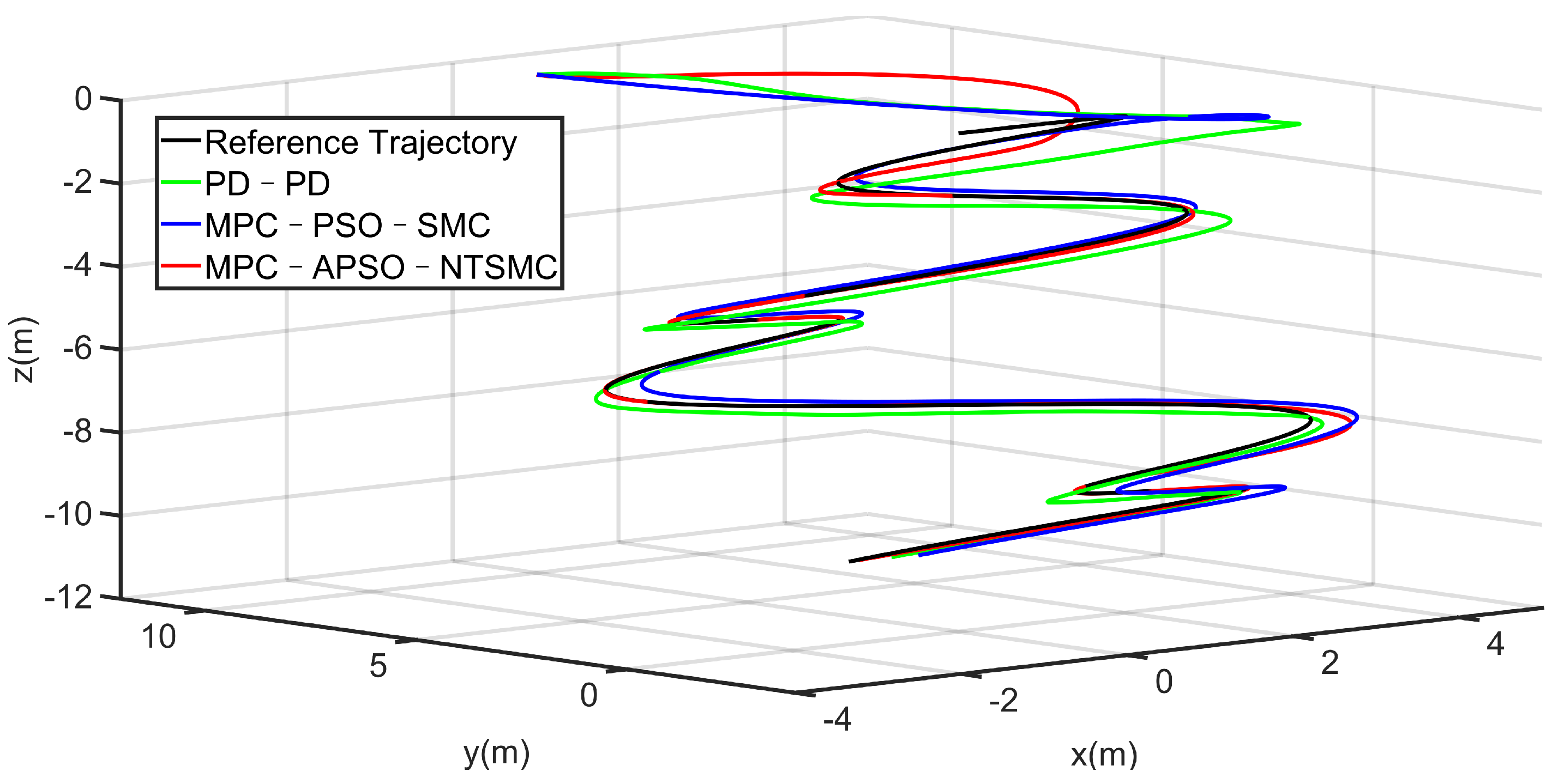
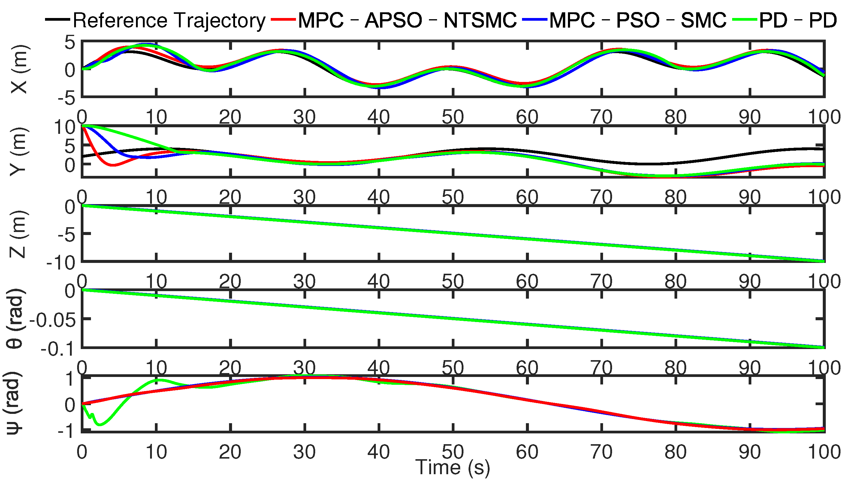
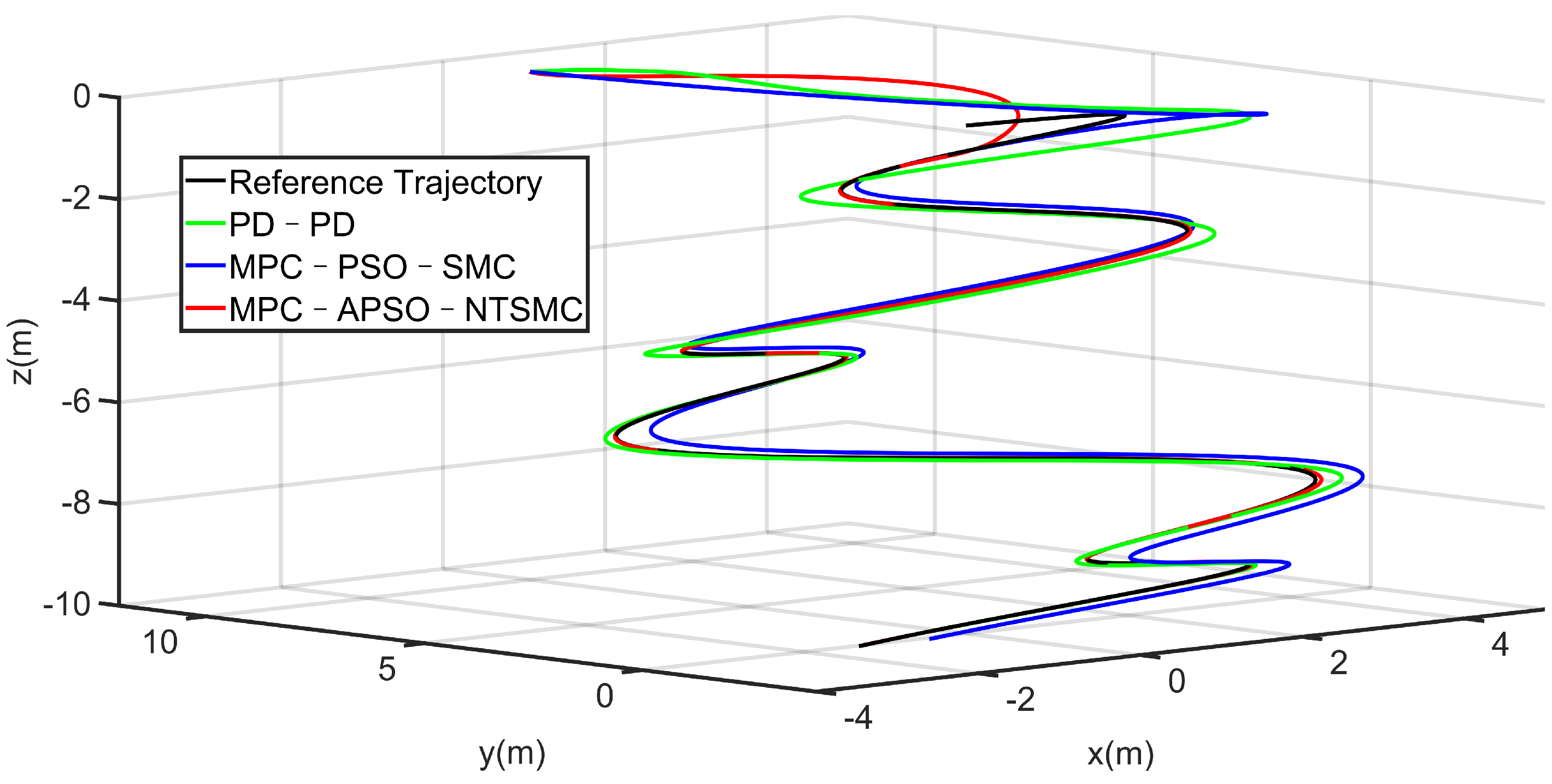
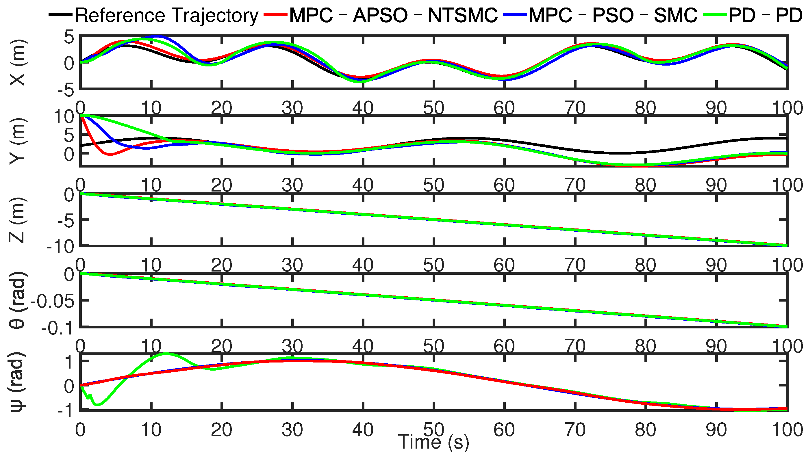
x d = 10 sin ( 0.1 t ) y d = 10 10 cos ( 0.1 t ) z d = 0.25 t θ d = 0.002 t ψ d = 0.1 t
It can be seen from Figure 9 and 
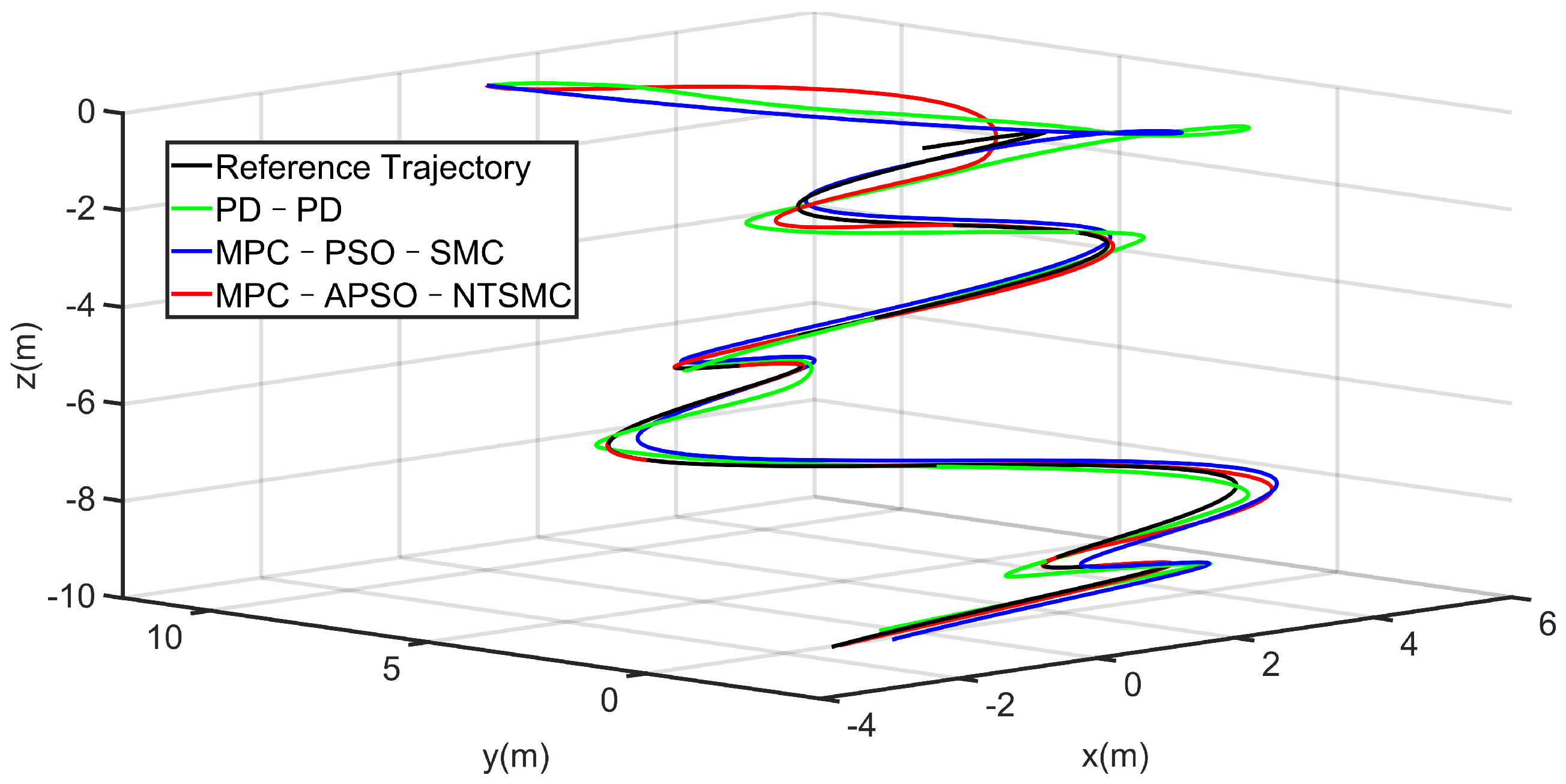
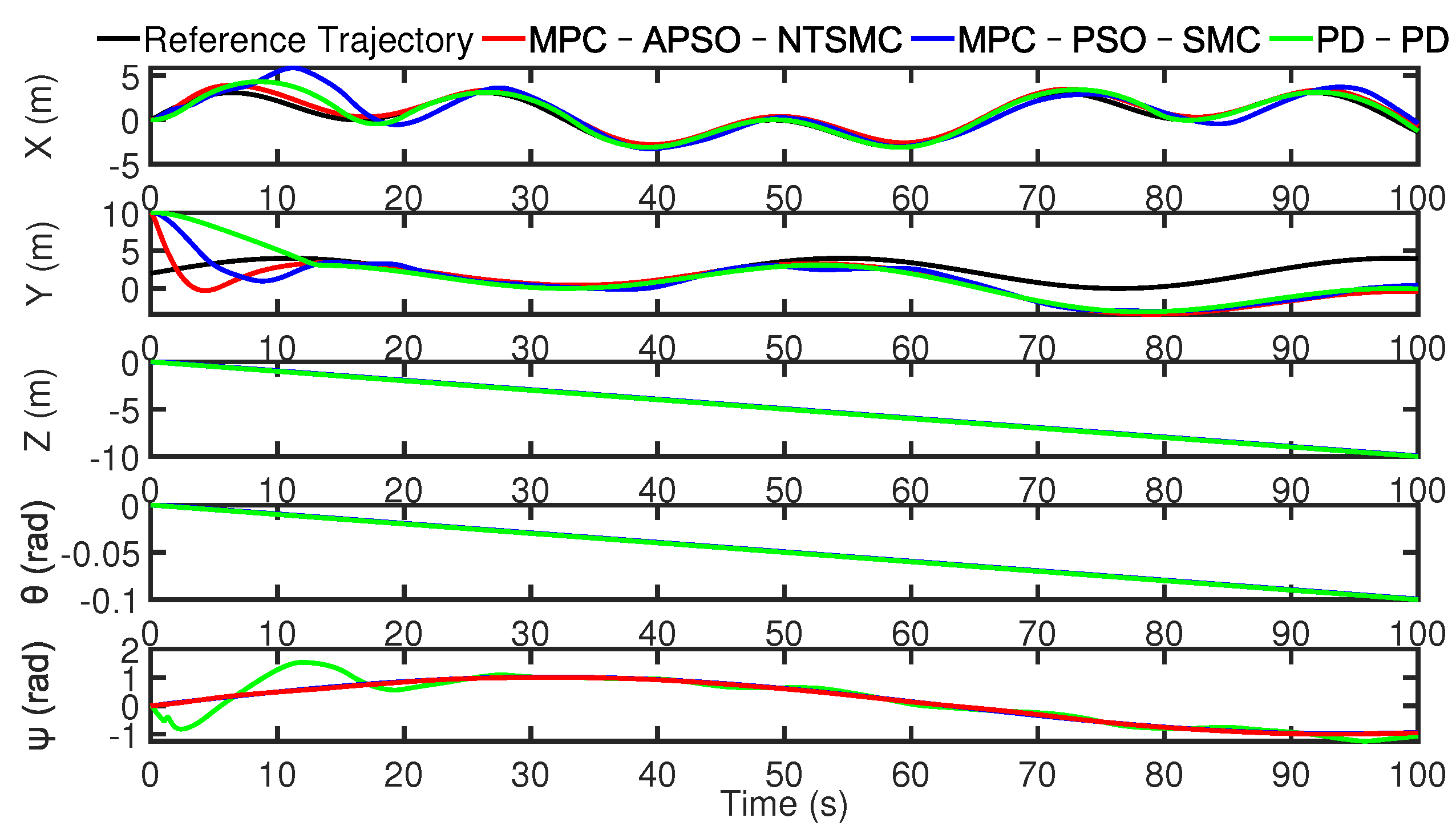
Figure 10 that all three controllers can provide better trajectory tracking performance for the AUV. However, since the AUV is a system with large inertia, the PD-PD controller (green curve) cannot track in time when the expected trajectory curvature of the AUV is large, resulting in relatively large tracking errors. In addition, the controller designed in this paper (red curve) has better final tracking performance than the MPC-PSO-SMC controller (blue curve) in terms of initial tracking speed and error control.
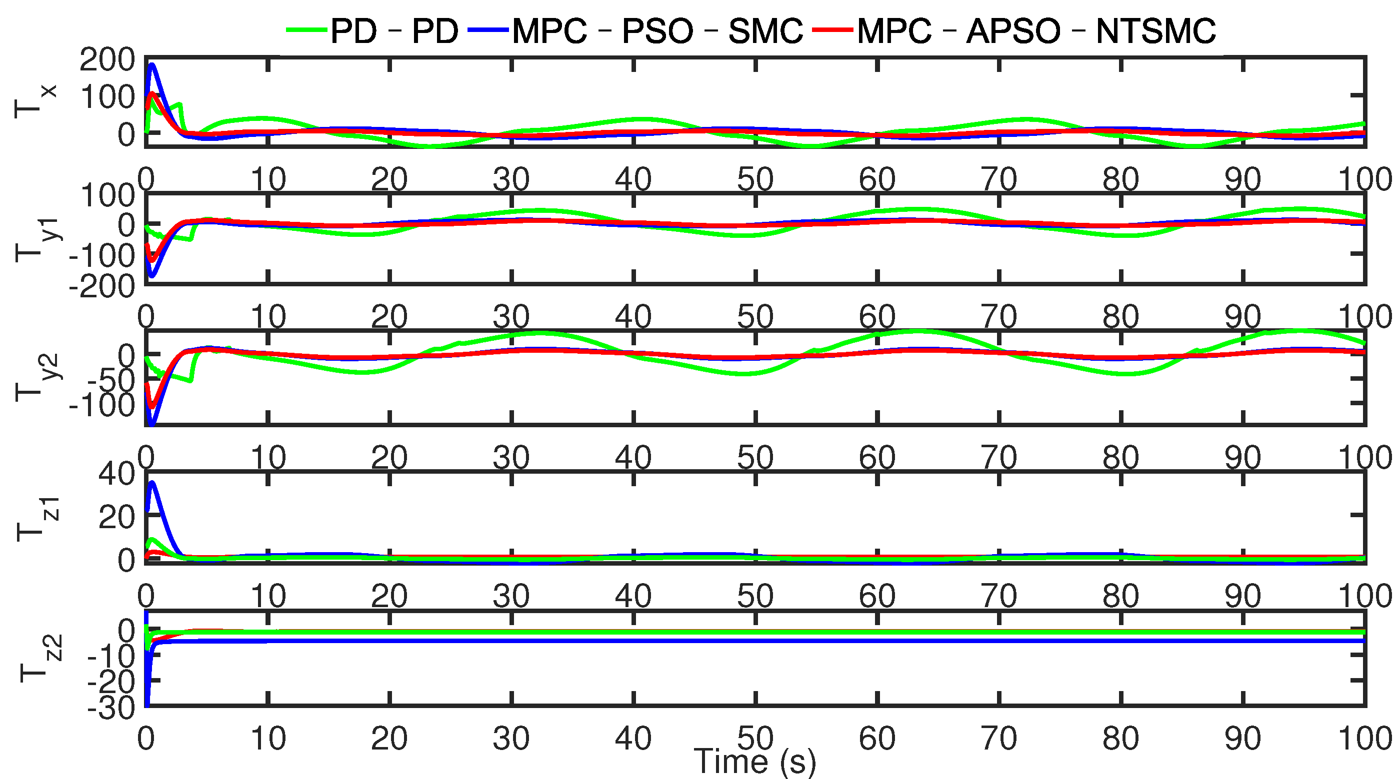
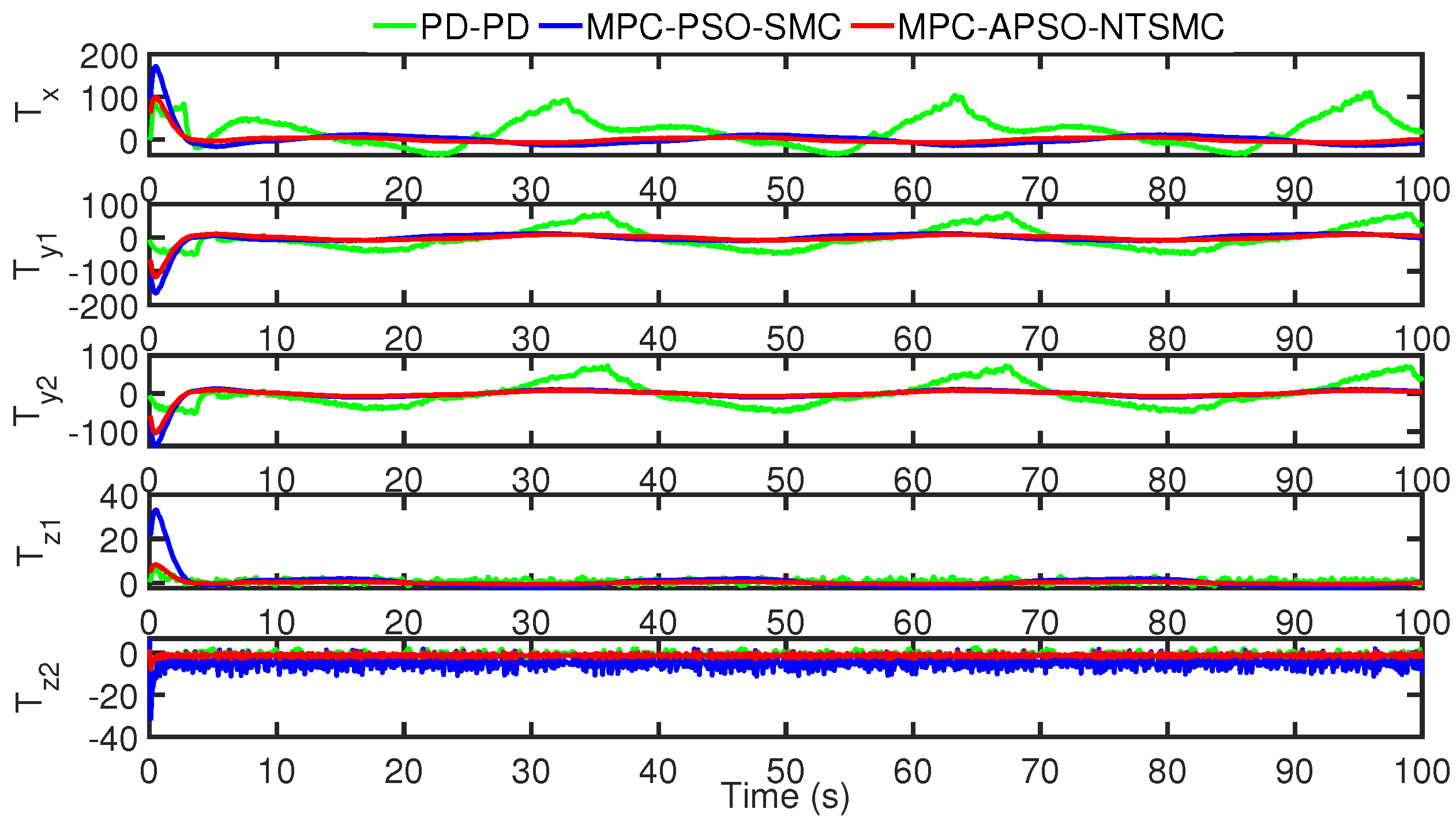
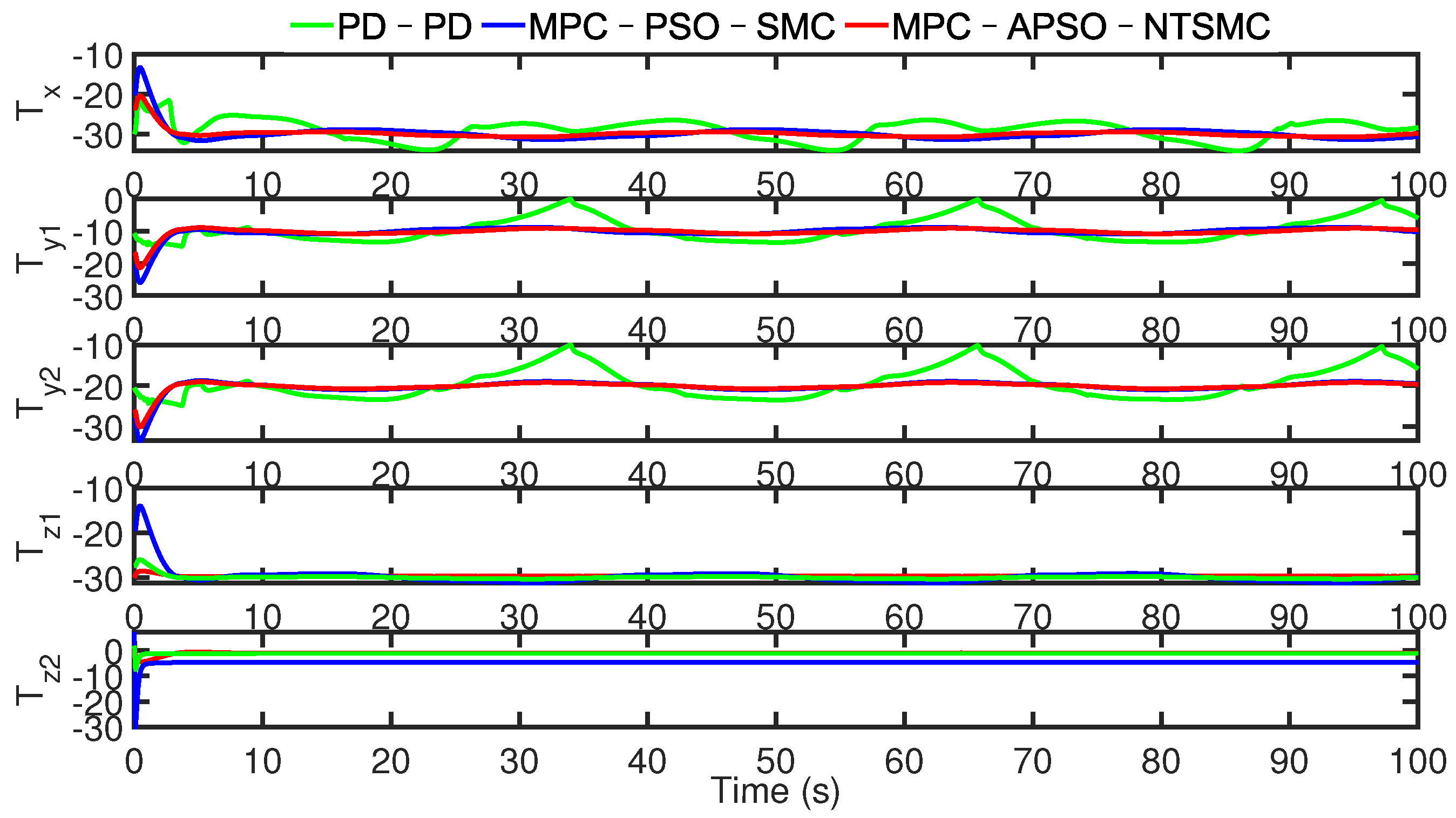
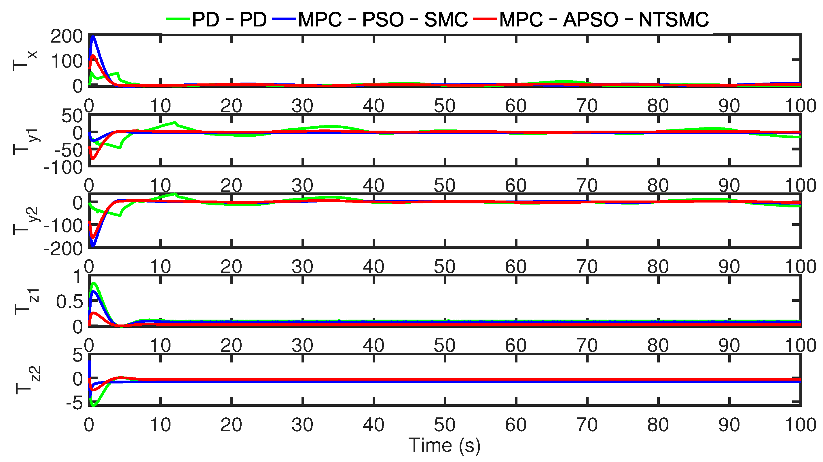
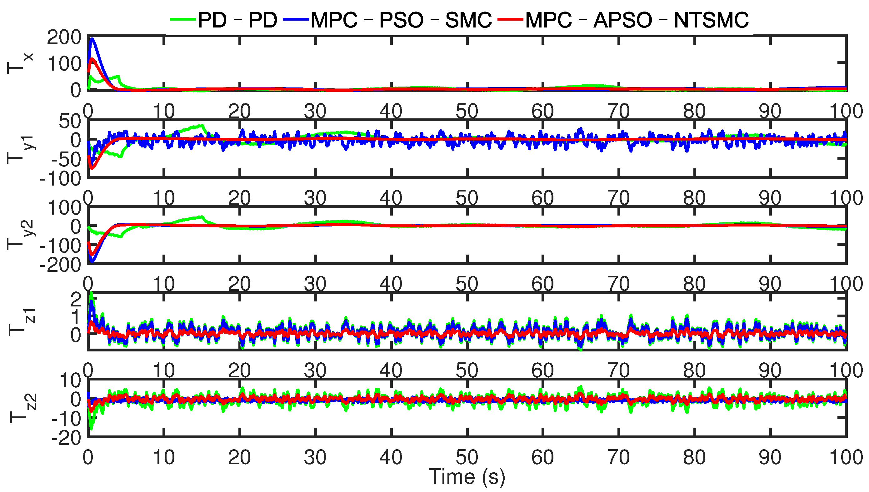
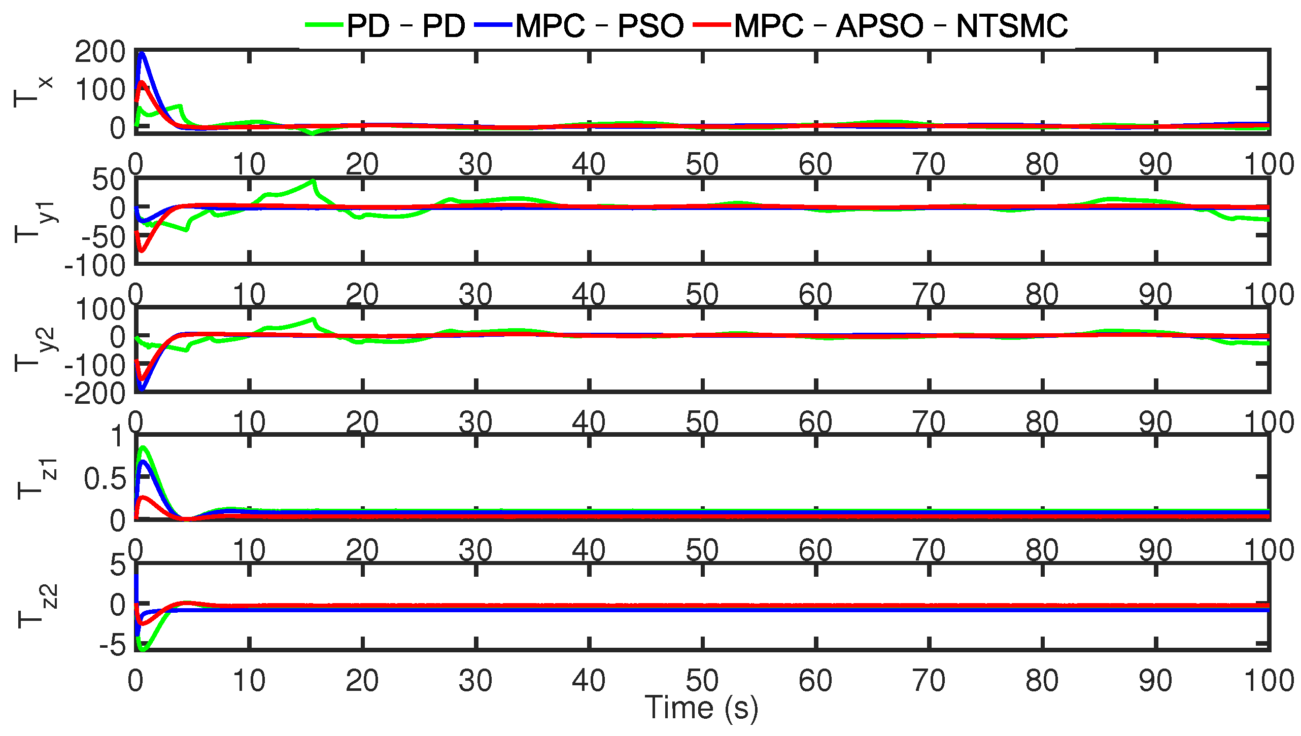
Figure 11 shows the thrust output of each thruster of the AUV during trajectory tracking. The figure shows that although the thrust output of the PD-PD controller (green curve) is not the maximum at the initial moment, the overall output fluctuates greatly, which is related to the difficulty of setting controller parameters. The controller proposed in this paper (red curve), under the action of the MPC-APSO kinematic controller and the NTSMC dynamics controller, has a relatively stable overall thrust output that is the best among the three.
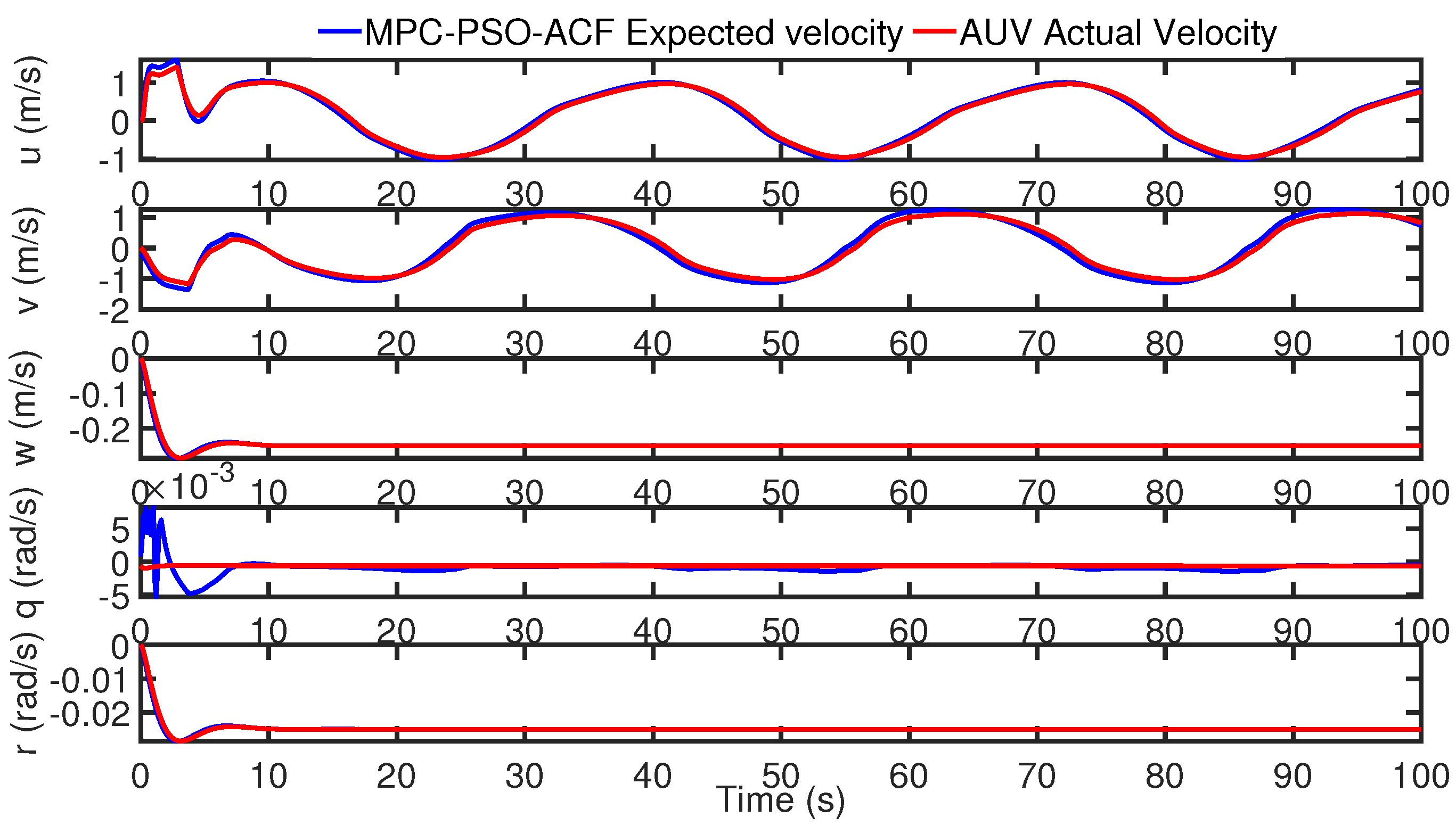
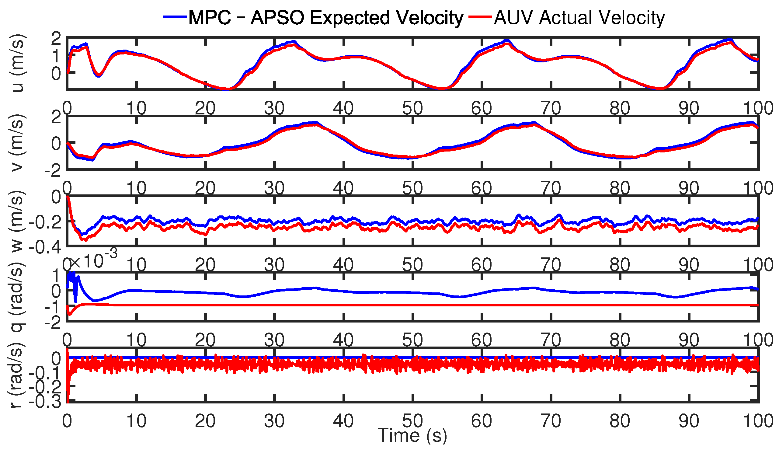
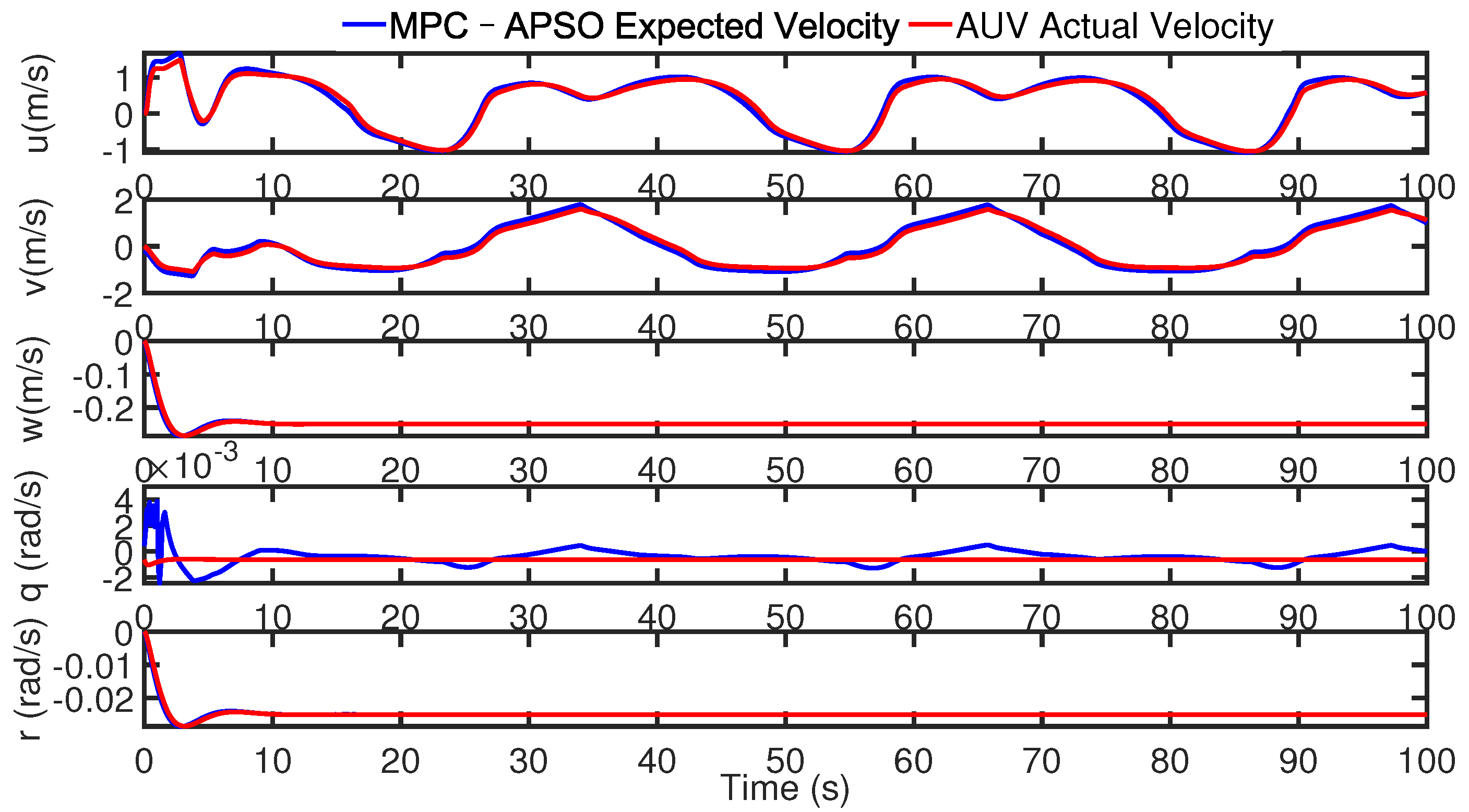
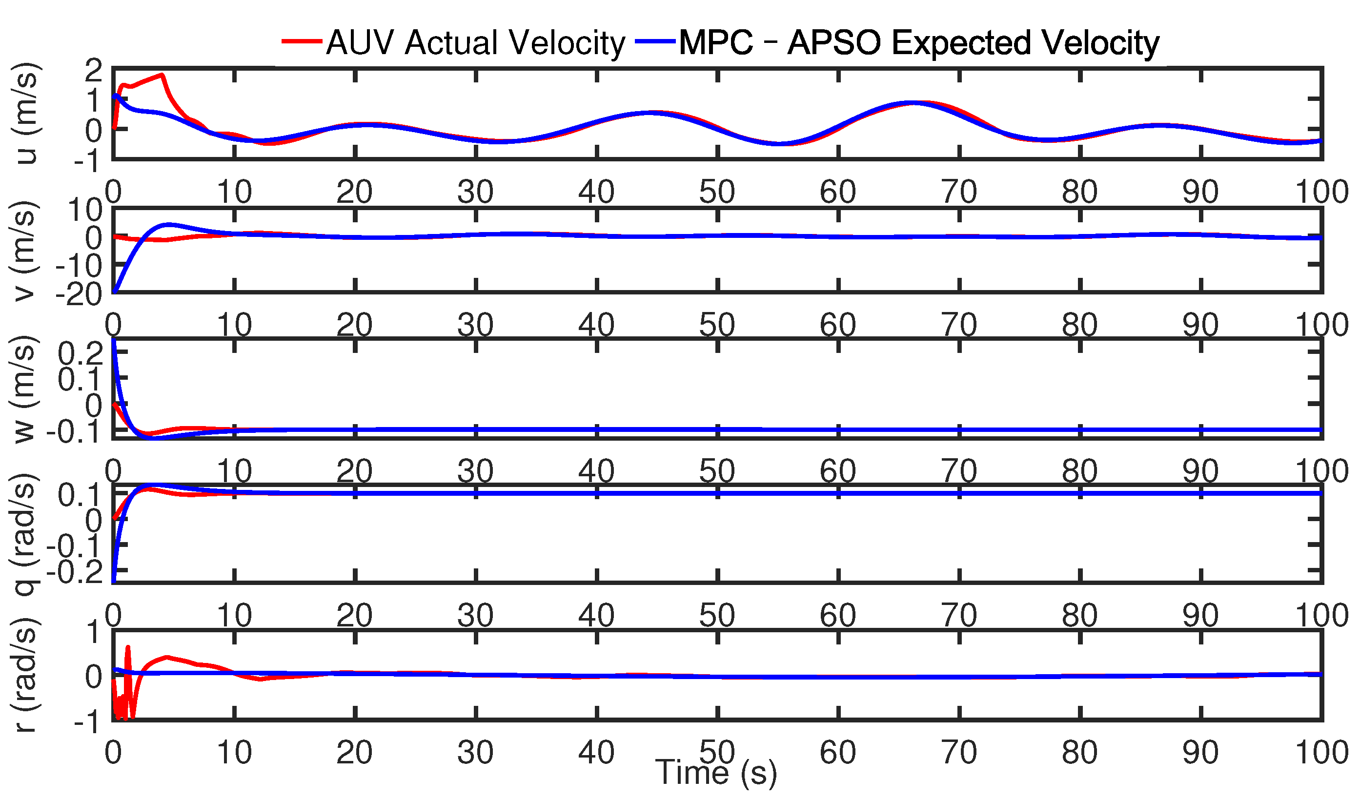
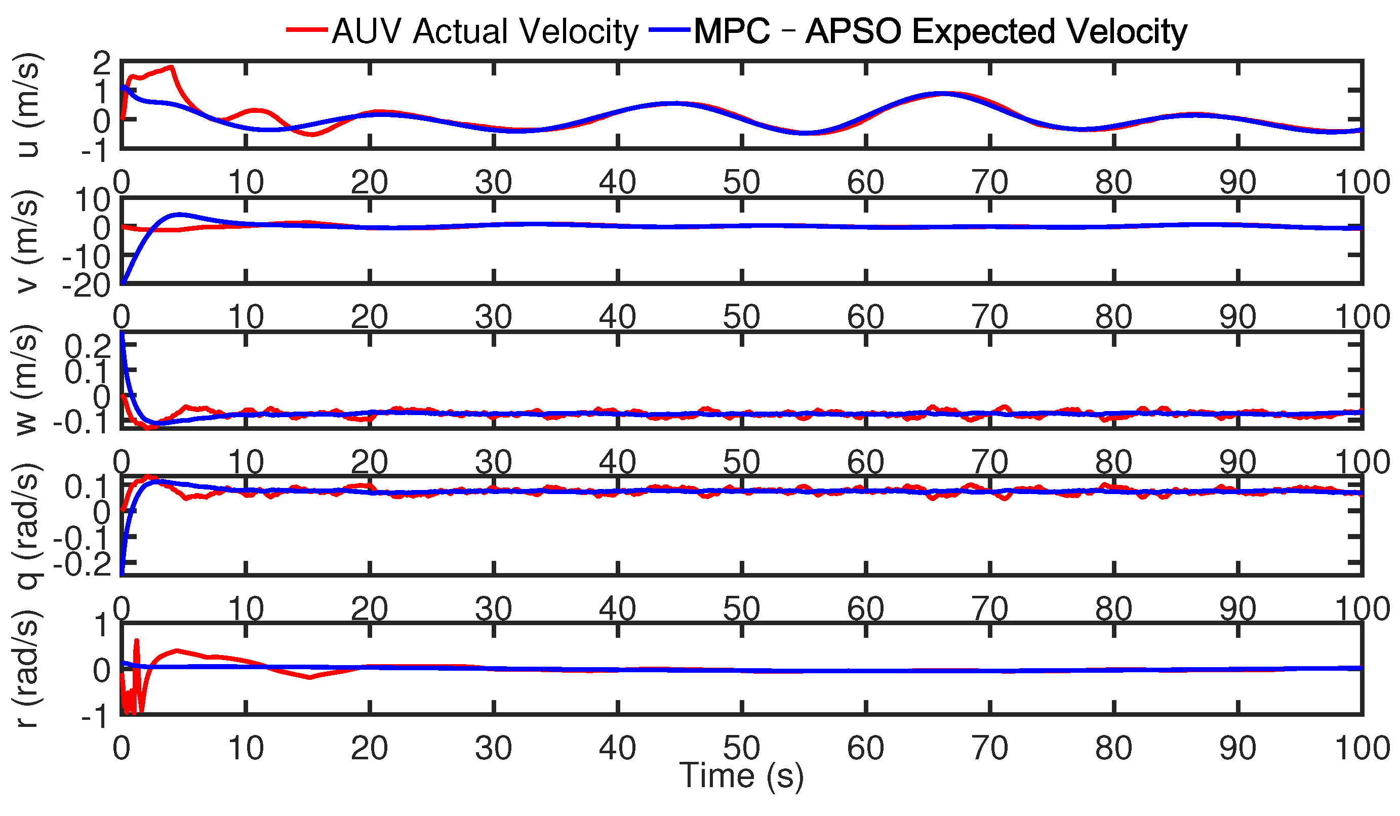
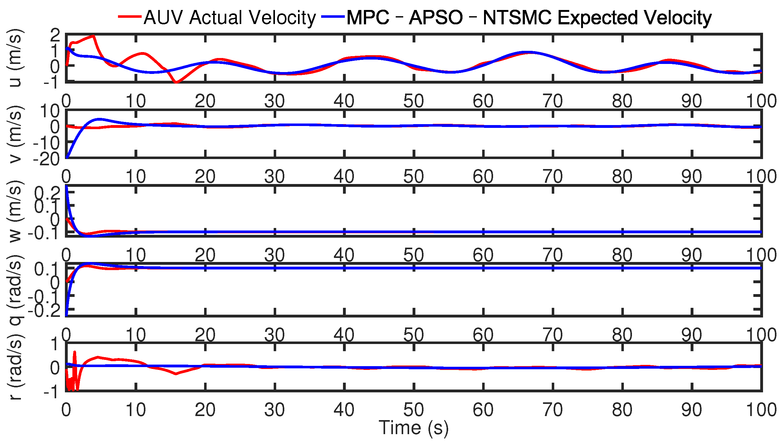
Figure 12 shows the effect of the NTSMC velocity controller tracking the optimal expected velocity command (blue curve) based on the RBF-NN compensator designed in this paper. Obviously, the MPC-APSO method proposed in this paper can obtain the globally optimal expected velocity, and the proposed velocity controller has a good tracking effect (red curve).
Table 3 shows the mean absolute error (MAE) data obtained by simulation when the AUV tracks the spiral trajectory proposed in Case 1 without disturbance. We can clearly draw from the data in the table that the MPC-APSO-NTSMC controller designed in this paper can make the trajectory tracking task of the AUV have the minimum position MAE. MAE data of pitch, roll, heave, pitch, and yaw positions were 0.1165 m, 0.2013 m, 0.1727 m, 0.0815 rad , and 0.0721 rad , respectively.
The simulation results of the three controllers for Case 1 with random disturbances are shown in Figure 13, Figure 14, Figure 15 and Figure 16.
Figure 13 shows 3D AUV tracking of a spiral trajectory with the influence of random disturbance. Obviously, compared with Case 1 without external disturbance, the tracking performance of the three control methods has declined, and the corresponding fluctuations are generated under the influence of random disturbance, which is reflected in the large changes to the trajectory curvature. However, compared with PD-PD (green curve) and MPC-PSO-SMC (blue curve), the proposed controller (red curve) still has the best tracking performance.
Figure 14 shows the trajectory tracking performance comparison of the three controllers for each degree of freedom. The PD-PD controller (green curve) has the largest error fluctuation. The proposed controller (red curve) under the action of the RBF-NN compensator not only improves the influence of model errors on the controller performance but also effectively compensates for external disturbance to minimize tracking error fluctuation and improve the robustness of the controller.
Figure 15 shows the comparison of simulation results of thruster thrust output in the case of random interference. Although the thrust output of the controller proposed in this paper has a small-amplitude oscillation with random interference, compared with the other two methods, the overall thrust output is relatively stable under the action of the MPC-APSO kinematic controller with the NTSMC dynamic controller. It is the best of the three.
Figure 16 shows the tracking of the velocity controller designed in this paper. The simulation results show that the velocity tracking performance of each degree of freedom of the AUV decreases slightly with random disturbance, but the overall tracking effect is good. At the same time, it can be proved that compared with the standard PSO, the APSO algorithm can obtain a global optimal value superior to the standard PSO in each sampling period of the MPC, and the proposed NTSMC velocity controller based on the RBF-NN compensator can effectively suppress the influence of external disturbances.
Table 4 shows the MAE data obtained by simulation when the AUV tracks the spiral trajectory proposed in Case 1 with random disturbances. We can also clearly draw from the data in the table that the MPC-APSO-NTSMC controller designed in this paper can make the trajectory tracking task of the AUV have the minimum position MAE. MAE data of surge, sway, heave, pitch, and yaw positions are 0.1678 m, 0.1913 m, 0.1427 m, 0.0775 rad , and 0.0903 rad , respectively.
In order to more fully consider the actual situation of underwater trajectory tracking of a fully actuated AUV, the wave and current interference is added in the simulation process, and the trajectory tracking control performance of PD-PD, MPC-PSO-NTSMC, and the proposed controller are again verified by simulation. The simulation results are shown in Figure 17, Figure 18, Figure 19 and Figure 20.
The results show that the proposed controller still has the best trajectory tracking performance and robustness, and all types of trajectory errors are the smallest among the three. The thrust output response speed is fast, the thrust output is smooth, and the speed tracking is correspondingly fast with the condition of wave and ocean current interference at the same time, which, again, proves the effectiveness and robustness of the controller (red curve).
Table 5 shows the MAE data obtained by simulation when the AUV tracks the spiral trajectory proposed in Case 1 with wave and current disturbance. We can clearly draw from the data in the table that the MPC-APSO-NTSMC controller designed in this paper can make the trajectory tracking task of the AUV have the minimum position MAE. MAE data of surge, roll, heave, pitch, and yaw are 0.1981 m, 0.1699 m, 0.1827 m, 0.0915 rad , and 0.0928 rad , respectively.
Case 2: We set the initial position of the fully actuated AUV in the underwater simulation environment to be η ( 0 ) = [ 0 , 10 , 0 , 0 , 0 ] T , and the function of the complex curve trajectory with time is defined as follows:
x d = 2 sin ( 0.1 t ) + 2 sin ( 0.3 t ) y d = 2 sin ( 0.05 t ) + 2 sin ( 0.15 t ) z d = 0.1 t θ d = 0.001 t ψ d = sin ( 0.015 π t )
Figure 21 and Figure 22 show the tracking performance of the AUV when tracking complex curves. It can be easily observed that the tracking errors of the three control methods under each degree of freedom increase significantly when tracking the trajectory of complex curves with multiple curvations, especially the position with large curvature changes, compared with tracking the spiral trajectory. However, the position tracking errors of the three control methods are all bounded. The overall tracking error result (red curve) of the proposed controller is better than that of the other two controllers.
Figure 23 shows the output of each thruster when the AUV tracks a complex curve. The PD-PD controller (green curve) has a large change rate of thruster output at the initial stage. Although the change rate of the MPC-PSO-SMC (blue curve) controller’s thruster output during the initial tracking process is better than that of the PD-PD controller, the output value is large. The proposed controller (red curve) has a minimum charge rate of thruster output during the entire tracking process, and it is relatively stable.
Figure 24 shows the effect of the NTSMC velocity controller based on the RBF-NN compensator designed in this paper to track the expected velocity command (blue curve). Obviously, the MPC-APSO method proposed in Case 2 can also obtain the globally optimal expected velocity, and the proposed velocity controller has a great tracking effect (red curve).
Table 6 shows the MAE data obtained by simulation when the AUV tracks the complex curve trajectory proposed in Case 2 without disturbance. We can also clearly draw from the data in the table that the MPC-APSO-NTSMC controller designed in this paper can make the trajectory tracking task of the AUV have the minimum position MAE. MAE data of surge, roll, heave, pitch, and yaw are 0.1778 m, 0.1845 m, 0.1025 m, 0.1134 rad , and 0.1219 rad , respectively.
Figure 25, Figure 26, Figure 27 and Figure 28 show the trajectory tracking performance of the AUV when tracking complex curves with random disturbance. Similar to tracking the spiral track, with the effect of the random disturbance, the controller proposed in this paper (red curve) can overcome the influence of tracking fluctuation caused by multi-curvature changes and random disturbance regardless of the overall tracking effect, the output stability of thrusters, and the velocity tracking effect of NTSMC based on the NN compensator. The effectiveness and robustness of the controller are the best of the three.
Table 7 shows the MAE data obtained by simulation when the AUV tracks the complex curve trajectory proposed in Case 2 with random disturbance. We can also clearly draw from the data in the table that the MPC-APSO-NTSMC controller designed in this paper can make the trajectory tracking task of the AUV have the minimum position MAE. MAE data of surge, roll, heave, pitch, and yaw are 0.1812 m, 0.1909 m, 0.1215 m, 0.1167 rad , and 0.1439 rad , respectively.
Figure 29, Figure 30, Figure 31 and Figure 32 show the trajectory tracking performance of the AUV when tracking complex curves with wave and current disturbance. Similar to spiral tracking, with the effect of the wave and current disturbance, the controller proposed in this paper (red curve) can overcome the influence of tracking fluctuation caused by multi-curvature changes and wave and current disturbance regardless of the overall tracking effect, the output stability of thrusters, and the velocity tracking effect of NTSMC based on the NN compensator. The effectiveness and robustness of the controller are still the best of the three.
Table 8 shows the MAE data obtained by simulation when the AUV tracks the complex curve trajectory proposed in Case 2 with wave and current disturbance. We can also clearly draw from the data in the table that the MPC-APSO-NTSMC controller designed in this paper can make the trajectory tracking task of AUV have the minimum position MAE. MAE data of surge, roll, heave, pitch, and yaw are 0.1843 m, 0.1712 m, 0.1901 m, 0.1004 rad , and 0.1115 rad , respectively.

5. Conclusions

Aiming at the problem of underwater 3D dynamic trajectory tracking control of fully actuated AUVs, a novel cascade controller using MPC and NTSMC is proposed in this paper. Firstly, the five-degree-of-freedom kinematics and dynamics model of the fully actuated AUV is established in the corresponding coordinate system. Secondly, a novel PSO method with adaptive inertia weight is proposed to replace the QP method for solving the optimal control sequence in standard MPC. Combined with the state and control input constraints of the AUV, MPC-APSO obtains the optimal velocity control sequence, generates the expected velocity command, and transmits it to the NTSMC velocity controller. The introduction of adaptive inertia weight can balance and improve the local search and global search capabilities of the optimization algorithm, which overcomes the problem of the traditional MPC control being unable to find the global optimal solution when using QP to solve for the optimal solution. After that, considering the modeling error of the dynamic model of AUV and the unknown disturbance of the underwater environment when the AUV performs underwater trajectory tracking control, this paper improves the response speed and control accuracy of NTSMC by designing an RBF-NN compensator. Moreover, stability analysis based on the Lyapunov method proves the stability of the two controllers. Finally, two different expected 3D trajectories are designed using MATLAB/Simulink to verify the dynamic trajectory tracking performance of the AUV with different external disturbances, and the robustness and effectiveness of the designed controller are verified.
In future research, we will focus on practical problems of AUVs in trajectory tracking control, such as the rationality of the expected trajectory, the integration of the constraints with the underwater environment and AUV dynamic constraints, controller input saturation, multi-AUV cooperative formation control, etc.

Author Contributions

Conceptualization, H.B. and H.Z.; methodology, H.B. and X.L.; software, H.B. and X.L.; formal analysis, H.B. and H.Z.; investigation, H.B. and H.Z.; data curation, H.B.; writing—original draft preparation, H.B. and J.L.; writing—review and editing, H.B. and H.Z.; visualization, H.B.; supervision, H.Z. and J.L. All authors have read and agreed to the published version of the manuscript.

Funding

This work was supported by the university–local integration category project “Underwater Vehicles Key Technology R&D Center” and the China Scholarship Council (grant no. 202006680065).

Data Availability Statement

Not applicable.

Conflicts of Interest

The authors declare no conflict of interest.

References

  1. Chu, Z.; Sun, B.; Zhu, D.; Zhang, M.; Luo, C. Motion control of unmanned underwater vehicles via deep imitation reinforcement learning algorithm. IET Intell. Transp. Syst. 2020, 14, 764–774. [Google Scholar] [CrossRef]
  2. Yin, J.; Wang, N. Predictive Trajectory Tracking Control of Autonomous Underwater Vehicles Based on Variable Fuzzy Predictor. Int. J. Fuzzy Syst. 2020, 23, 1809–1822. [Google Scholar] [CrossRef]
  3. Rahmani, M.; Rahman, M.H. New hybrid control of autonomous underwater vehicles. Int. J. Control. 2021, 94, 3038–3045. [Google Scholar] [CrossRef]
  4. Xie, T.; Li, Y.; Jiang, Y.; An, L.; Wu, H. Backstepping active disturbance rejection control for trajectory tracking of underactuated autonomous underwater vehicles with position error constraint. Int. J. Adv. Robot. Syst. 2020, 17, 1729881420909633. [Google Scholar] [CrossRef] [Green Version]
  5. Ru, J.; Yu, S.; Wu, H.; Li, Y.; Wu, C.; Jia, Z.; Xu, H. A Multi-AUV Path Planning System Based on the Omni-Directional Sensing Ability. J. Mar. Sci. Eng. 2021, 9, 806. [Google Scholar] [CrossRef]
  6. Jia, C.; Chen, Z.; Zhang, G.; Shi, L.; Sun, Y.; Pang, S. AUV Tunnel Tracking Method Based on Adaptive Model Predictive Control. In Proceedings of the IOP Conference Series: Materials Science and Engineering; IOP Publishing: Bristol, UK, 2018; Volume 428, p. 012070. [Google Scholar]
  7. Cao, X.; Sun, H.; Guo, L. Potential field hierarchical reinforcement learning approach for target search by multi-AUV in 3-D underwater environments. Int. J. Control. 2020, 93, 1677–1683. [Google Scholar] [CrossRef]
  8. Liu, X.; Zhang, M.; Chen, Z. Trajectory tracking control based on a virtual closed-loop system for autonomous underwater vehicles. Int. J. Control. 2020, 93, 2789–2803. [Google Scholar] [CrossRef]
  9. Bechlioulis, C.P.; Karras, G.C.; Heshmati-Alamdari, S.; Kyriakopoulos, K.J. Trajectory tracking with prescribed performance for underactuated underwater vehicles under model uncertainties and external disturbances. IEEE Trans. Control. Syst. Technol. 2016, 25, 429–440. [Google Scholar] [CrossRef]
  10. Liu, X.; Zhang, M.; Yao, F.; Chu, Z. Observer-based region tracking control for underwater vehicles without velocity measurement. Nonlinear Dyn. 2022, 108, 3543–3560. [Google Scholar] [CrossRef]
  11. An, R.; Guo, S.; Zheng, L.; Hirata, H.; Gu, S. Uncertain moving obstacles avoiding method in 3D arbitrary path planning for a spherical underwater robot. Robot. Auton. Syst. 2022, 151, 104011. [Google Scholar] [CrossRef]
  12. Gao, Z.; Guo, G. Command filtered finite-time formation tracking control of AUVs with unknown control directions. IET Control. Theory Appl. 2020, 14, 1744–1751. [Google Scholar] [CrossRef]
  13. Rober, N.; Hammond, M.; Cichella, V.; Martin, J.E.; Carrica, P. 3D path following and L1 adaptive control for underwater vehicles. Ocean Eng. 2022, 253, 110971. [Google Scholar] [CrossRef]
  14. Shen, C.; Shi, Y.; Buckham, B. Integrated path planning and tracking control of an AUV: A unified receding horizon optimization approach. IEEE/ASME Trans. Mechatron. 2016, 22, 1163–1173. [Google Scholar] [CrossRef]
  15. Zhou, B.; Su, Y.; Huang, B.; Wang, W.; Zhang, E. Trajectory tracking control for autonomous underwater vehicles under quantized state feedback and ocean disturbances. Ocean Eng. 2022, 256, 111500. [Google Scholar] [CrossRef]
  16. Min, F.; Pan, G.; Xu, X. Modeling of autonomous underwater vehicles with multi-propellers based on maximum likelihood method. J. Mar. Sci. Eng. 2020, 8, 407. [Google Scholar] [CrossRef]
  17. García-Molleda, D.; Sandoval, J.; Coria, L.N.; Bugarin, E. Energy-based trajectory tracking control for underwater vehicles subject to disturbances with actuator partial faults and bounded input. Ocean Eng. 2022, 248, 110666. [Google Scholar] [CrossRef]
  18. Sun, Y.; Zhang, C.; Zhang, G.; Xu, H.; Ran, X. Three-dimensional path tracking control of autonomous underwater vehicle based on deep reinforcement learning. J. Mar. Sci. Eng. 2019, 7, 443. [Google Scholar] [CrossRef] [Green Version]
  19. Liu, X.; Zhang, M.; Wang, Y.; Rogers, E. Design and experimental validation of an adaptive sliding mode observer-based fault-tolerant control for underwater vehicles. IEEE Trans. Control. Syst. Technol. 2018, 27, 2655–2662. [Google Scholar] [CrossRef]
  20. Hong, L.; Wang, X.; Zhang, D.; Xu, H. Numerical Study on Hydrodynamic Coefficient Estimation of an Underactuated Underwater Vehicle. J. Mar. Sci. Eng. 2022, 10, 1049. [Google Scholar] [CrossRef]
  21. Liang, X.; Qu, X.; Wang, N.; Zhang, R.; Li, Y. Three-dimensional trajectory tracking of an underactuated AUV based on fuzzy dynamic surface control. IET Intell. Transp. Syst. 2020, 14, 364–370. [Google Scholar] [CrossRef]
  22. Sarhadi, P.; Noei, A.R.; Khosravi, A. Model reference adaptive PID control with anti-windup compensator for an autonomous underwater vehicle. Robot. Auton. Syst. 2016, 83, 87–93. [Google Scholar] [CrossRef]
  23. Hammad, M.M.; Elshenawy, A.K.; El Singaby, M. Trajectory following and stabilization control of fully actuated AUV using inverse kinematics and self-tuning fuzzy PID. PLoS ONE 2017, 12, e0179611. [Google Scholar] [CrossRef] [PubMed] [Green Version]
  24. Yan, Y.; Yu, S. Sliding mode tracking control of autonomous underwater vehicles with the effect of quantization. Ocean Eng. 2018, 151, 322–328. [Google Scholar] [CrossRef]
  25. Guo, X.; Yan, W.; Cui, R. Neural network-based nonlinear sliding-mode control for an AUV without velocity measurements. Int. J. Control. 2019, 92, 677–692. [Google Scholar] [CrossRef]
  26. Elmokadem, T.; Zribi, M.; Youcef-Toumi, K. Trajectory tracking sliding mode control of underactuated AUVs. Nonlinear Dyn. 2016, 84, 1079–1091. [Google Scholar] [CrossRef] [Green Version]
  27. Londhe, P.; Patre, B. Adaptive fuzzy sliding mode control for robust trajectory tracking control of an autonomous underwater vehicle. Intell. Serv. Robot. 2019, 12, 87–102. [Google Scholar] [CrossRef]
  28. Eski, İ.; Yildirim, S. Design of neural network control system for controlling trajectory of autonomous underwater vehicles. Int. J. Adv. Robot. Syst. 2014, 11, 7. [Google Scholar] [CrossRef] [Green Version]
  29. Shen, C.; Shi, Y.; Buckham, B. Trajectory tracking control of an autonomous underwater vehicle using Lyapunov-based model predictive control. IEEE Trans. Ind. Electron. 2017, 65, 5796–5805. [Google Scholar] [CrossRef]
  30. Li, X.; Zhu, D. An adaptive SOM neural network method for distributed formation control of a group of AUVs. IEEE Trans. Ind. Electron. 2018, 65, 8260–8270. [Google Scholar] [CrossRef]
  31. Zhang, Y.; Liu, X.; Luo, M.; Yang, C. MPC-based 3-D trajectory tracking for an autonomous underwater vehicle with constraints in complex ocean environments. Ocean Eng. 2019, 189, 106309. [Google Scholar] [CrossRef]
  32. Shen, C.; Buckham, B.; Shi, Y. Modified C/GMRES algorithm for fast nonlinear model predictive tracking control of AUVs. IEEE Trans. Control. Syst. Technol. 2016, 25, 1896–1904. [Google Scholar] [CrossRef]
  33. Yan, Z.; Gong, P.; Zhang, W.; Wu, W. Model predictive control of autonomous underwater vehicles for trajectory tracking with external disturbances. Ocean Eng. 2020, 217, 107884. [Google Scholar] [CrossRef]
  34. Bao, H.; Zhu, H. Modeling and Trajectory Tracking Model Predictive Control Novel Method of AUV Based on CFD Data. Sensors 2022, 22, 4234. [Google Scholar] [CrossRef]
  35. Gan, W.; Zhu, D.; Ji, D. QPSO-model predictive control-based approach to dynamic trajectory tracking control for unmanned underwater vehicles. Ocean Eng. 2018, 158, 208–220. [Google Scholar] [CrossRef]
  36. Kemna, S.; Hamilton, M.; Hughes, D.T.; LePage, K.D. Adaptive autonomous underwater vehicles for littoral surveillance: The GLINT10 field trial results. Intell. Serv. Robot. 2011, 4, 245. [Google Scholar] [CrossRef]
  37. Zhong, Y.; Yang, Y.; He, K.; Chen, C. Fast terminal sliding-mode control based on unknown input observer for the tracking control of underwater vehicles. Ocean Eng. 2022, 264, 112480. [Google Scholar] [CrossRef]
  38. Zhang, J.; Xiang, X.; Zhang, Q.; Li, W. Neural network-based adaptive trajectory tracking control of underactuated AUVs with unknown asymmetrical actuator saturation and unknown dynamics. Ocean Eng. 2020, 218, 108193. [Google Scholar] [CrossRef]
Figure 1. Reference frames.
Jmse 10 01867 g001
Figure 2. Schematic diagram of propeller arrangement.
Jmse 10 01867 g002
Figure 3. Mesh result.
Jmse 10 01867 g003
Figure 4. Velocity cloud diagram and convergence process of CFD simulation.
Jmse 10 01867 g004
Figure 5. Fitting results.
Jmse 10 01867 g005
Figure 6. Schematic diagram of thrust curve.
Jmse 10 01867 g006
Figure 7. Diagram of the fully actuated AUV control strategy.
Jmse 10 01867 g007
Figure 8. Simulation model.
Jmse 10 01867 g008
Figure 9. AUV spiral trajectory tracking without disturbance for Case 1.
Jmse 10 01867 g009
Figure 10. Position tracking performance for the tracking task without disturbance for Case 1.
Jmse 10 01867 g010
Figure 11. The thrust of thrusters for the tracking task without disturbance for Case 1.
Jmse 10 01867 g011
Figure 12. Velocity tracking of the AUV without disturbance for Case 1.
Jmse 10 01867 g012
Figure 13. AUV spiral trajectory tracking with random disturbance for Case 1.
Jmse 10 01867 g013
Figure 14. Position tracking performancesfor the tracking task with random disturbance for Case 1.
Jmse 10 01867 g014
Figure 15. The thrust of thrusters for the tracking task with random disturbance for Case 1.
Jmse 10 01867 g015
Figure 16. Velocity tracking of the AUV with random disturbance for Case 1.
Jmse 10 01867 g016
Figure 17. AUV spiral trajectory tracking with wave and current disturbance for Case 1.
Jmse 10 01867 g017
Figure 18. Position tracking performancesfor the tracking task with wave and current disturbance for Case 1.
Jmse 10 01867 g018
Figure 19. The thrust of thrusters for the tracking task with wave and current disturbance for Case 1.
Jmse 10 01867 g019
Figure 20. Velocity tracking for the AUV with wave and current disturbance for Case 1.
Jmse 10 01867 g020
Figure 21. AUV complex curve trajectory tracking without disturbance for Case 2.
Jmse 10 01867 g021
Figure 22. Position tracking performance for the tracking task without disturbance for Case 2.
Jmse 10 01867 g022
Figure 23. The thrust of thrusters for the tracking task without disturbance for Case 2.
Jmse 10 01867 g023
Figure 24. Velocity tracking for the AUV without disturbance for Case 2.
Jmse 10 01867 g024
Figure 25. AUV complex curve trajectory tracking with random disturbance for Case 2.
Jmse 10 01867 g025
Figure 26. Position tracking performance for the tracking task with random disturbance for Case 2.
Jmse 10 01867 g026
Figure 27. The thrust of thrusters for the tracking task with random disturbance for Case 2.
Jmse 10 01867 g027
Figure 28. Velocity tracking for the AUV with random disturbance for Case 2.
Jmse 10 01867 g028
Figure 29. AUV complex curve trajectory tracking with wave and current disturbance for Case 2.
Jmse 10 01867 g029
Figure 30. Position tracking performance for the tracking task with wave and current disturbance for Case 2.
Jmse 10 01867 g030
Figure 31. The thrust of thrusters for the tracking task with wave and current disturbance for Case 2.
Jmse 10 01867 g031
Figure 32. Velocity tracking for the AUV with wave and current disturbance for Case 2.
Jmse 10 01867 g032
Table 1. Basic parameters and hydrodynamic coefficients of AUV.
ParameterValueParameterValue
Mass183 kgDiameter0.4 m
Length2.5 m I y 56.1 kgm 2
X u ˙ 35.78 kg I z 54.5 kgm 2
Y v ˙ 159.26 kg X u 5.77 kg / s
Z w ˙ 151.31 kg Y v 37.13 kg / s
M q ˙ 39.29 kgm 2 Z w 35.94 kg / s
N r ˙ 41.71 kgm 2 M q 10.71 kgm 2 / ( s · rad )
X u u 17.77 kg / m N r 9.96 kgm 2 / ( s · rad )
Y v v 150.23 kg / m M q q 26.55 kgm 2 / rad 2
Z w w 147.76 kg / m N r r 26.71 kgm 2 / rad 2
Table 2. Simulation parameters.
ParameterValueParameterValue
T100 s T s 100
Y m a x [ , , , π / 2 , π ] T N m a x 50
Y m i n [ , , , π / 2 , π ] T c 1 2.05
v m a x [ 2 , 2 , 2 , 0.5 , 0.5 ] T c 2 2.05
v m i n [ 2 , 2 , 2 , 0.5 , 0.5 ] T N p s 100
τ m a x [ 135 , 270 , 270 , 20 , 20 ] T N p 10
τ m i n [ 90 , 180 , 180 , 20 , 20 ] T N c 4
Γ Δ v d i a g ( 1 , 1 , 1 , 1 , 1 ) Υ m a x 0.9
Γ x d i a g ( 0.05 , 0.05 , 0.05 , 0.05 , 0.05 ) Υ m i n 0.4
Δ v m a x [ 0.15 , 0.1 , 0.1 , 0.05 , 0.05 ] T n15
Δ v m i n [ 0.15 , 0.1 , 0.1 , 0.05 , 0.05 ] T
Table 3. Position MAE without disturbance after 20 s for Case 1.
Methodsx (m)y (m)z (m) θ (rad) ψ (rad)
PD-PD0.28970.24450.29170.15470.1529
MPC-PSO-SMC0.15700.13170.21840.10920.1291
MPC-APSO-NTSMC0.11650.20130.17270.08150.0721
Table 4. Position MAE with random disturbance after 20 s for Case 1.
Methodsx (m)y (m)z (m) θ (rad) ψ (rad)
PD-PD0.33120.32390.30070.18350.2025
MPC-PSO-SMC0.20180.19170.23540.11240.1301
MPC-APSO-NTSMC0.16780.19130.14270.07750.0903
Table 5. Position MAE with wave and current disturbance after 20 s for Case 1.
Methodsx (m)y (m)z (m) θ (rad) ψ (rad)
PD-PD0.35780.27890.22190.19490.1825
MPC-PSO-SMC0.19650.21170.27840.12990.1791
MPC-APSO-NTSMC0.19810.16990.18270.09160.0928
Table 6. Position MAE without disturbance after 20 s for Case 2.
Methodsx (m)y (m)z (m) θ (rad) ψ (rad)
PD-PD0.31120.23220.20010.17480.1698
MPC-PSO-SMC0.24570.22340.25310.14060.1818
MPC-APSO-NTSMC0.17780.18450.10250.11340.1219
Table 7. Position MAE with random disturbance after 20 s for Case 2.
Methodsx (m)y (m)z (m) θ (rad) ψ (rad)
PD-PD0.34570.28120.23210.19040.1717
MPC-PSO-SMC0.25120.23310.25830.15670.1896
MPC-APSO-NTSMC0.18120.19090.12150.11670.1439
Table 8. Position MAE with wave and current disturbance after 20 s for Case 2.
Methodsx (m)y (m)z (m) θ (rad) ψ (rad)
PD-PD0.35490.26890.23390.15490.1634
MPC-PSO-SMC0.18740.22010.24010.13370.1814
MPC-APSO-NTSMC0.18430.17120.19010.10040.1115
Publisher’s Note: MDPI stays neutral with regard to jurisdictional claims in published maps and institutional affiliations.

