Taking into Account the Eddy Density on Analysis of Underwater Glider Motion

Abstract

Mesoscale eddies play an important role in regulating the global ocean ecosystem and climate variability. However, few studies have been found to focus on the survey of the underwater gliders (UGs) motion performance inside mesoscale eddies. The dynamic model of an UG considering the eddy density is established to predict its motion performance inside an eddy. Ignoring the effect of vertical velocity inside the eddy on the motion of UG, the simulation results and experimental data are compared to verify the derived model. From the analysis of the motion performance, the vertical velocity is larger at 400∼940 m depth than that at a depth of 0∼400 m in the ascent. Considering the vertical structures of parameters within eddies, the climbing profiles are chosen as the available samples to capture an eddy better. The larger error caused by the eddy density mainly occurs near the depth of the thermocline. Moreover, there is a stronger influence of eddy density on the motion performance of the UG in the ascent than that in the descent. The results show the differences in the effect of the mesoscale eddy density on the motion performance of “Petrel II” UG in the descent and ascent, and they provide a sampling suggestion for the application of UGs in the mesoscale eddy observation.

1. Introduction

Mesoscale eddies with horizontal scales of 50∼500 km and temporal scales of 10∼100 days [1] exist ubiquitously in the ocean. By trapping water parcels, mesoscale eddies advect nutrients and water properties away from the regions of eddy origins [2]. As a considerable contributor to the transport of nutrients, phytoplankton [2], heat and salt [3], mesoscale eddies play an important role in regulating the global ocean ecosystem and climate variability [4]. However, the high variability in spatial and temporal dynamics of mesoscale eddies makes their in situ observation a great challenge. As a new type of ocean-sampling platform, UGs characterized by the high sampling resolution and long endurance provide submesoscale resolving along their trajectory [5,6] and continuous long-term observation [7,8], making their application in the investigation of the mesoscale eddy a hotspot [4,9,10,11,12,13,14,15,16]. Previous attempts have indicated that the density distribution within mesoscale eddies varies complicatedly [17,18,19,20], which will considerably influence the motion performance of UGs.

To predict the movement, maneuverability and stability of UGs, substantial work has been completed from their dynamic modeling to behavior analysis. Leonard et al. presented the nonlinear dynamic model of UGs and thoroughly analyzed their movement, stability and controllability in the vertical plane. Based on the analysis results, the feedback control laws of the UGs were carefully designed [21,22,23]. Woolsey et al. also carried out the UG dynamic behavior analysis and control strategy development [24,25], in which an optimal control law with minimal energy consumption was sought [26,27]. More than that, by considering the influence of ocean currents, a nonlinear multi-body dynamic model of the UG for the non-uniform flow fields was established [28]. In order to analyze the motion performance of an UG with independently controllable main wings, Arima et al. constructed the dynamic model of the UG and clarified its hydrodynamic performance and motion capability through various kinds of experiments and numerical simulation respectively [29,30]. Isa et al. proposed a dynamic model of a hybrid-driven UG based on Newton–Euler formulation and investigated its motion performance with a well-designed Neural Network Predictive Control (NNPC) in the presence of water currents [31]. Using the Gibbs–Appell equations, Wang et al. formulated the dynamic model of an UG and developed the linear quadratic regulator (LQR) and the $H\infty$ robust controller to ensure the UG’s favorable performance with parameter uncertainties [32]. Liu et al. adopted the differential geometry theory to establish the dynamic model of a hybrid-driven UG. Based on the model, they discussed the ‘’zigzag” motion characteristics of the UG and compared the simulation results with the sea trial data to verify the validity of the model [33]. Zhang et al. conducted a comprehensive study on the spiral motion of an UG in which the spiral motion characteristics of the UG under the influence of strong ocean currents were elucidated by comparing with the results from sea trials [34]. Considering the hull deformation and seawater density variation, Yang et al. obtained the full dynamic model of a deep-sea UG using the Newton–Euler method. Compared with the simpler dynamic model that ignored the hull deformation and seawater density variation, the superiority of the full dynamic model in truly reflecting the dynamic behaviors of the UG was validated [35]. Wang et al. introduced the parameter of ocean depth into the motion equations of a dual-buoyancy-driven full ocean depth UG. The dynamic model of the UG was derived using the Newton–Euler formulation and vector mechanics theory in light of the surrounding seawater density and the deep contraction of the UG and seawater, which were expressed as the functions of the seawater pressure and temperature. Based on the model, the gliding and steering performance of the UG were analyzed in detail [36]. Although a lot of studies the literature have reported the dynamic models of the UGs in various forms and analyses of their dynamic behavior, the researchers mainly tried to establish the proper model of different UGs and analyze their dynamic motion in static water or flow fields. Very few studies have been found to focus on the investigation of the UGs motion performance inside mesoscale eddies.

The South China Sea, as the largest and deepest marginal sea surrounded by the Asian continent and the islands of Kalimantan, Palawan, Luzon, and Taiwan in the western North Pacific Ocean, has a very complex submarine topography. The Asian monsoon system and its interactions with the coastline and submarine topography result in rich mesoscale eddies in the South China Sea. However, our understanding of the UGs motion performance inside mesoscale eddies remains incomplete. To reveal the motion characteristics of UGs within eddies, thus verify the effectiveness of their application in observing mesoscale eddies, and guide the design of a sampling scheme for mesoscale eddies observation, it is necessary to establish the dynamic model of the UG and simulate its motion process within an eddy. From 4 August 2017 to 29 August 2017, twelve “Petrel II” UGs developed by Tianjin University, China, were deployed in the northern part of the South China Sea, acquiring 1720 profiles totally. In this paper, the CTD (Conductivity-Temperature-with-Depth profiler) dataset collected by UGs and satellite data of SLA (Sea Level Anomaly) distributed by CMEMS (Copernicus Marine Environment Monitoring Service) are integrated. On this basis, we investigated the density distribution within the anticyclonic eddy, developed the dynamic model of “Petrel II” UG considering the buoyancy variation affected by both the density distribution within the eddy and deformation of the pressure hull, and conducted the analysis of the UG motion performance inside the eddy.

This paper is organized as follows: Section 2 describes the dynamic modeling of “Petrel II” UG, including kinematical modeling and force analysis, during which the density distribution within the eddy and deformation of the UG hull expressed as functions of ocean depth are introduced into the buoyancy analysis. Section 3 investigates the dynamic behavior of “Petrel II” UG inside the anticyclonic eddy based on the constructed dynamic model. Section 4 summarizes the full paper.

2. Materials and Methods

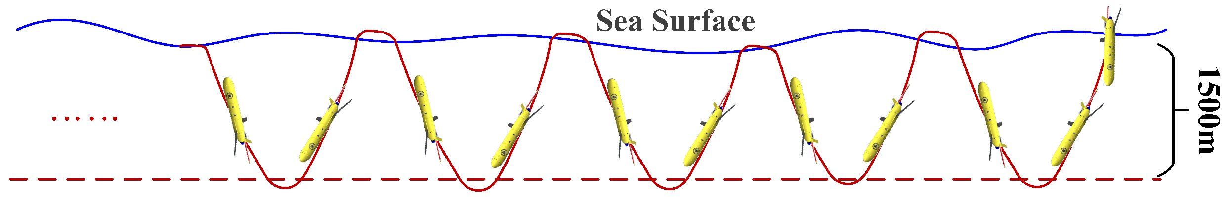
UGs, characterized by long operation range (up to several thousand kilometers), long endurance (up to months), low costs and repeatable utilization, are driven by the buoyancy to move vertically and the lift produced by the fixed wings to achieve horizontal movement, thus traveling in a sawtooth trajectory beneath the sea surface. During diving or climbing through the water column, UGs collect various measurements, including temperature, conductivity, dissolved oxygen, current, fluorescence of chlorophyll, sound, etc., depending on the equipped sensors. The “Petrel II” UGs (Figure 1) developed by Tianjin University, China were applied in the research. “Petrel II” UG can be equipped with multiple physical and biochemical sensors, such as a CTD sensor, vector hydrophone, background hydrophone, current meter, MicroRider and optical backscatter. Each dive cycle of the UG took about 4∼5 h to reach up to 1500 m depth vertically and cover about 4∼5 km horizontally, which is not constant, as the presence of intense currents may impact it. The performance of “Petrel II” gliders has been validated in repeated sea trials [37].

2.1. Kinematical Modeling

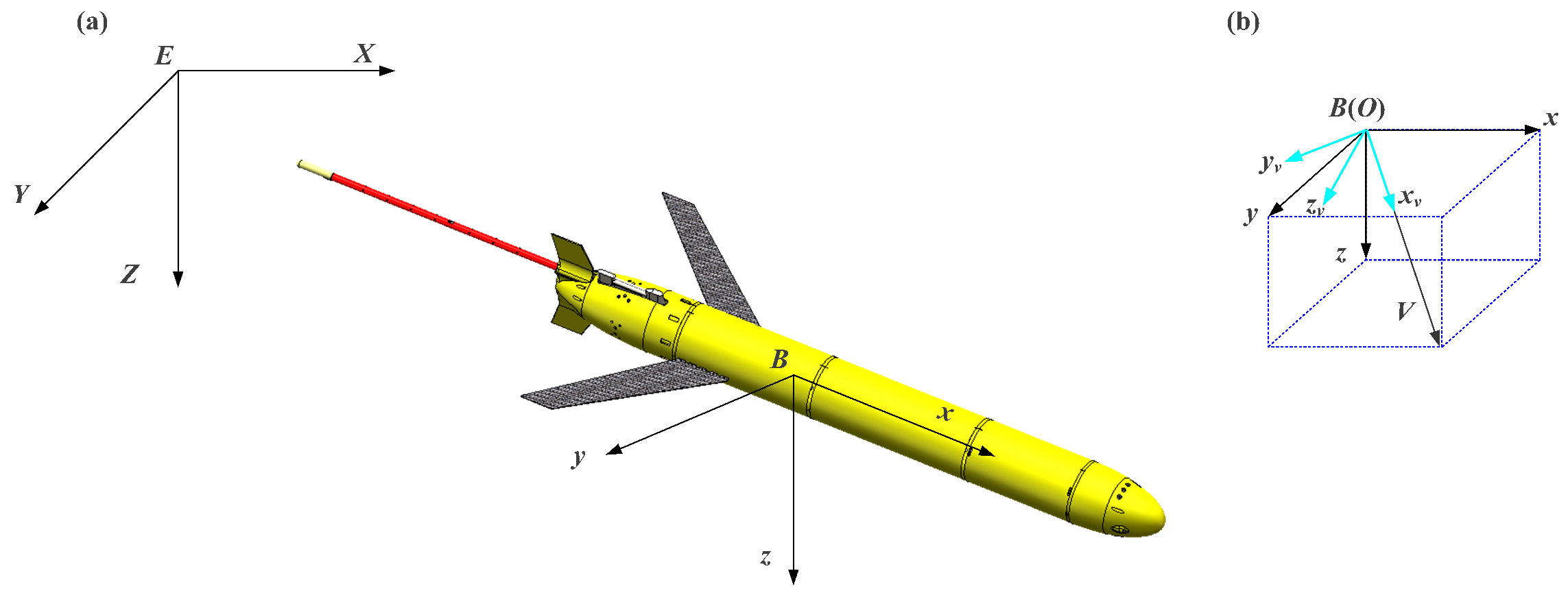
To establish the kinematical model of “Petrel II” UG, three reference frames of the UG, including the inertial frame, the body frame and the velocity frame, are firstly chosen (see Figure 2). The entry point of the UG is chosen as the origin of the inertial frame E-XYZ, in which the EX-axis locates in the horizontal plane and points to the north, the EZ-axis, perpendicular to the horizontal plane, points downward, and the EY-axis satisfies the right-hand rule. The body frame B-xyz, fixed on the UG, locates the buoyancy center of the UG, with the Bx-axis pointing to the fore along its longitudinal axis, the By-axis, perpendicular to the Bx-axis, pointing to the starboard side of the UG, and the direction of the Bz-axis determined by the right-hand rule. Similar to the body frame, the velocity frame O-$x_v{y}_v{z}_v$ also selects the buoyancy center as its origin, with the $O{x}_v$-axis pointing forward along the velocity, the $O{z}_v$-axis in the Bxz plane, perpendicular to the $O{x}_v$-axis, and the direction of the $O{y}_v$-axis meeting the right-hand rule.

In the body frame, the linear velocity V of “Petrel II” UG is expressed as ${[u,v,w]}^T$

$$\left\{\begin{array}{c}V=\sqrt{u^2+v^2+w^2}\\ \alpha =arctan\left(\frac{w}{u}\right)\\ \beta =arcsin\left(\frac{v}{V}\right)\end{array}\right.$$

(1)

where $\alpha$ is the angle of attack, and $\beta$ represents the sideslip angle.

The origin of the body frame in the inertial frame is represented as ${[X,Y,Z]}^T$, and thus, its velocity will be shown as ${[\dot{X}, \dot{Y}, \dot{Z}]}^T$. The transformation between ${[\dot{X}, \dot{Y}, \dot{Z}]}^T$ and ${[u,v,w]}^T$ can be expressed as follows:

$$\left\{\begin{array}{c}\dot{X}=ucos\theta cos\psi +vsin\theta cos\psi sin\phi -vsin\psi cos\phi \\ +wsin\theta cos\psi cos\phi +wsin\psi sin\phi \\ \dot{Y}=ucos\theta sin\psi +vsin\theta sin\psi sin\phi +vcos\psi cos\phi \\ +wsin\theta sin\psi cos\phi -wcos\psi sin\phi \\ \dot{Z}=-usin\theta +vcos\theta sin\phi +wcos\theta cos\phi \end{array}\right.$$

(2)

The angular velocity in the inertial frame is given in the form of

$$\left[\begin{array}{c}\dot{\phi }\\ \dot{\theta }\\ \dot{\psi }\end{array}\right]=\left[\begin{array}{ccc}1& sin\phi tan\theta & cos\phi tan\theta \\ 0& cos\phi & -sin\phi \\ 0& sin\phi /cos\theta & cos\phi /cos\theta \end{array}\right]\left[\begin{array}{c}p\\ q\\ r\end{array}\right]$$

(3)

where the vector ${[p,q,r]}^T$ stands for the angular velocity in the body frame. By integrating Equations (1)–(3), the kinematical model of “Petrel II” UG is derived.

2.2. Force Analysis

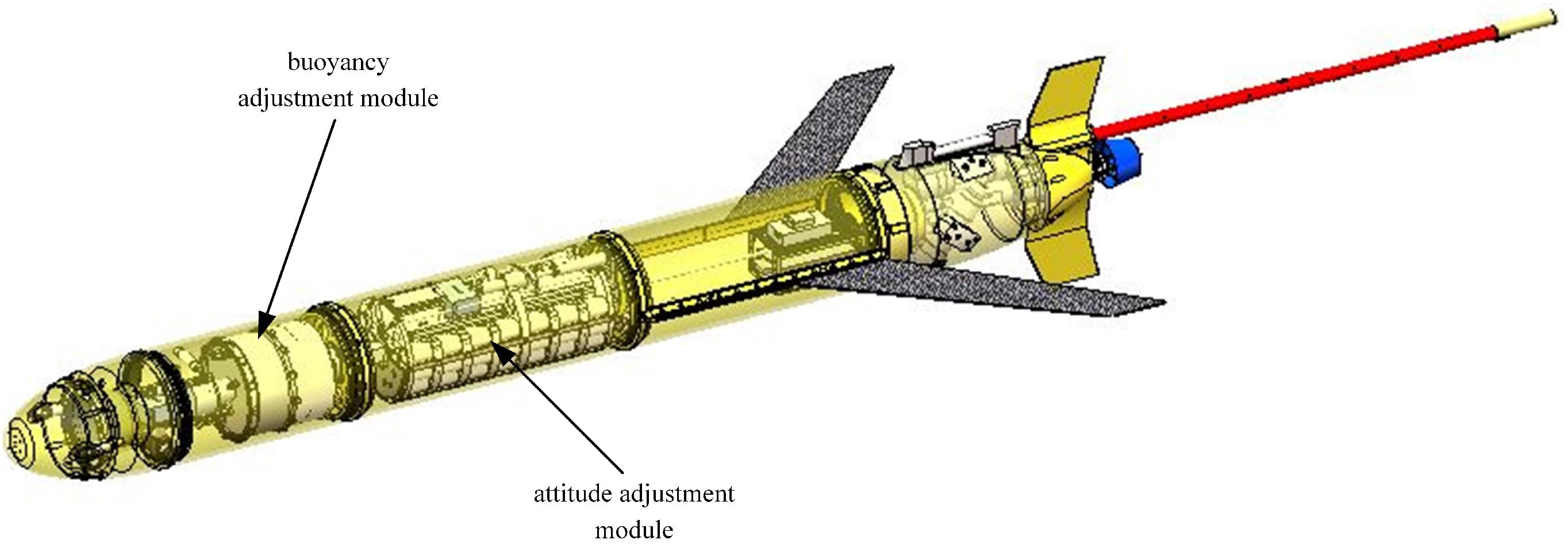
The “Petrel II” UG is composed of the main body (including the pressure hull, two wings, antenna and other appendages), the buoyancy adjustment module and the attitude adjustment module (shown in Figure 3). The mass center of the main body does not coincide with the buoyancy center, and in general, the mass is expressed as m_m. By changing the displaced volume of the UG, the buoyancy adjustment module produces the required buoyancy with the buoyancy center located at the Bx-axis [38], which is represented as m_b. The battery package with the mass denoted as m_p adjusts the attitude by moving along and rotating around the Bx-axis to change the pitch angle and roll angle, respectively. The external forces acting on the UG during its navigation include hydrodynamic force and other external forces (including buoyancy and gravity).

2.2.1. Buoyancy

The buoyancy is denoted as B₀.

$$B_0=\rho g{V}_0$$

(4)

where $\rho$ represents the density of seawater and $V_0$ means the displaced volume when the UG is adjusted to neutral buoyancy before entering the water. The buoyancy $B_0$ is determined by $\rho$ and $V_0$, and it points upward in the inertial frame.

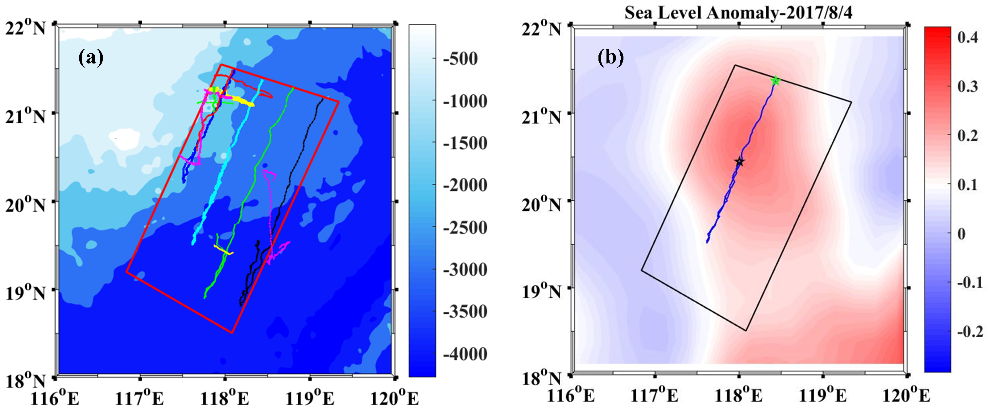
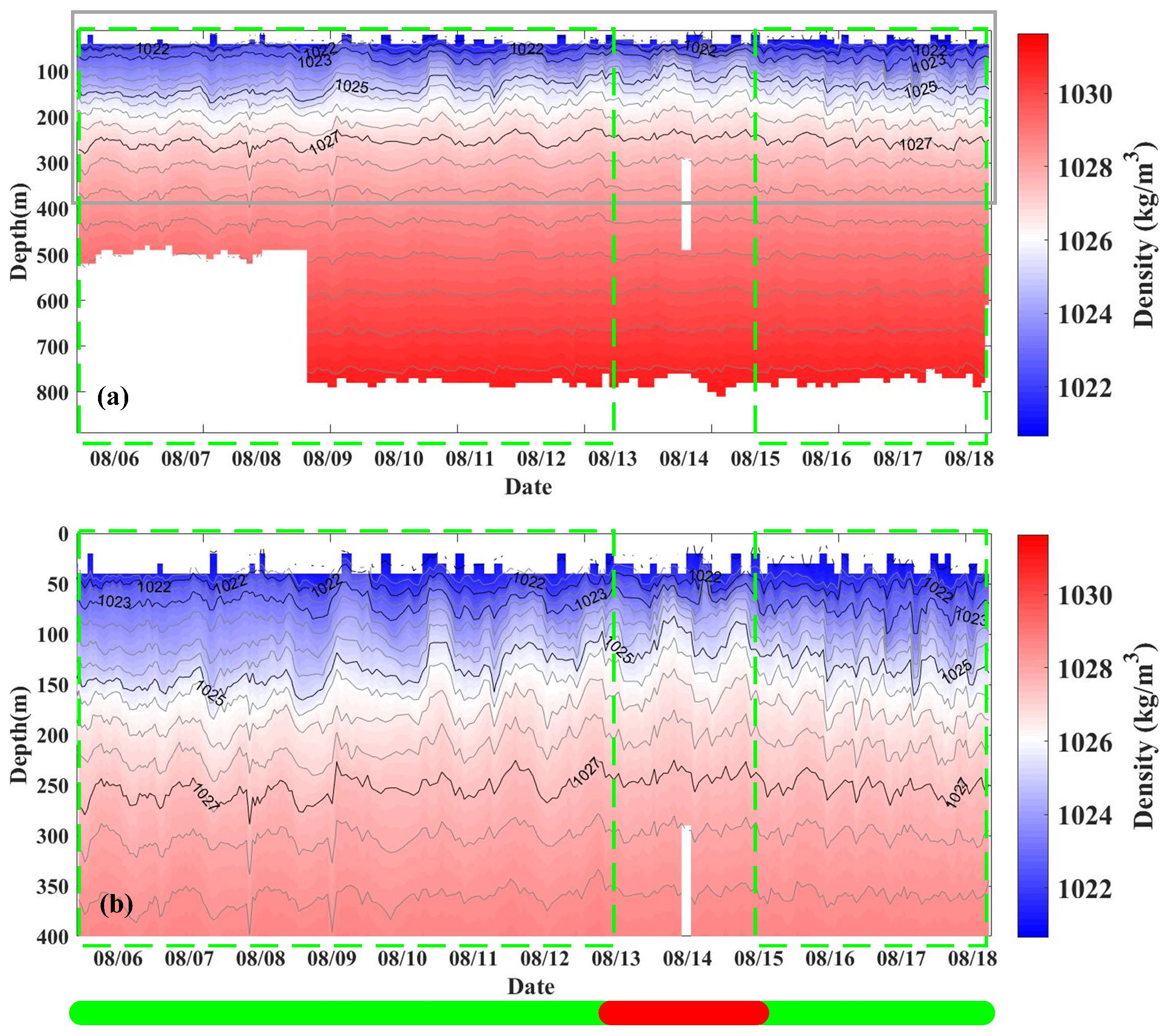
The density increases gradually with the increasing depth due to the steady stratification in most seas [39]. When an anticyclonic mesoscale eddy exists, the density stratification of the sea varies correspondingly. In August 2017, a multi-parameter observation for a mesoscale eddy using twelve “Petrel II” UGs in the northern part of the South China Sea was carried out by Tianjin University, China (see Figure 4a) [40]. Among the UGs, UG No. 6 (described as UG 6 in the following sections) collected ocean parameters from August 5 to August 18, sailing for 14 days and 360.3 km, during which UG 6 crossed the center of the anticyclonic mesoscale eddy and acquired 121 profiles about the eddy totally. The trajectory of UG 6 is presented in Figure 4b where the green and black stars represent the entry and recovery point of the UG 6, respectively.

Equipped with a SeaBird Glider Payload CTD, UG 6 collected ocean parameters of conductivity, temperature and pressure. The sampling frequency of the CTD was set to be 0.25 HZ, and the vertical resolution of the sampling was about 0.8 m with a mean vertical speed of 0.2 m/s. The observation accuracy of the sensor was ±0.002 °C for temperature, ±0.0003 S/m for conductivity and $\pm 0.1\%$ for pressure. The manufacturer has performed the preliminary calibration of the CTD. Before the trial, the CTD was calibrated again at National Ocean Technology Center, Tianjin, China. After the mission, the raw data were downloaded from the internal memory of the UG and then processed. The quality control, validation and smoothness of the data collected by UG 6 have been completed in the previous work [4]. The density of seawater is calculated by the method recorded in the reference [41]. Thus, the density distribution along the trajectory of UG 6 is revealed (shown in Figure 5). According to the previous work [42], the eddy parameters such as positions, radius, and amplitude were carefully identified from the SLA (downloaded from CMEMS) map. From Figure 4b, UG 6 crossed the eddy during its mission. Thus, the density distribution within an eddy is displayed in Figure 5. For brevity, the identification of the eddy will not be described in the paper.

In Figure 5a, the density increases from 1020.0 kg/m³ (near the sea surface) to 1031.6 kg/m³ (depth < 900 m) with the increase of depth. Near the depth of 100 m, a sinking of isopycnals can be seen obviously, indicating that the presence of the anticyclonic eddy changes the steady stratification of seawater. To better display the density distribution within the eddy, the upper water column of 0∼400 m is isolated from the whole depth, as shown in Figure 5b. From August 13 to 15 (marked as the red bar below Figure 5b), UG 6 sailed outside the eddy and took transects inside the eddy during the rest time (marked as the green bar). In Figure 5b, the isopycnals present a bowl-shaped descending, where the closer the isopycnals are to the eddy center, the deeper they descend, while the farther they are to the eddy center, the shallower they descend.

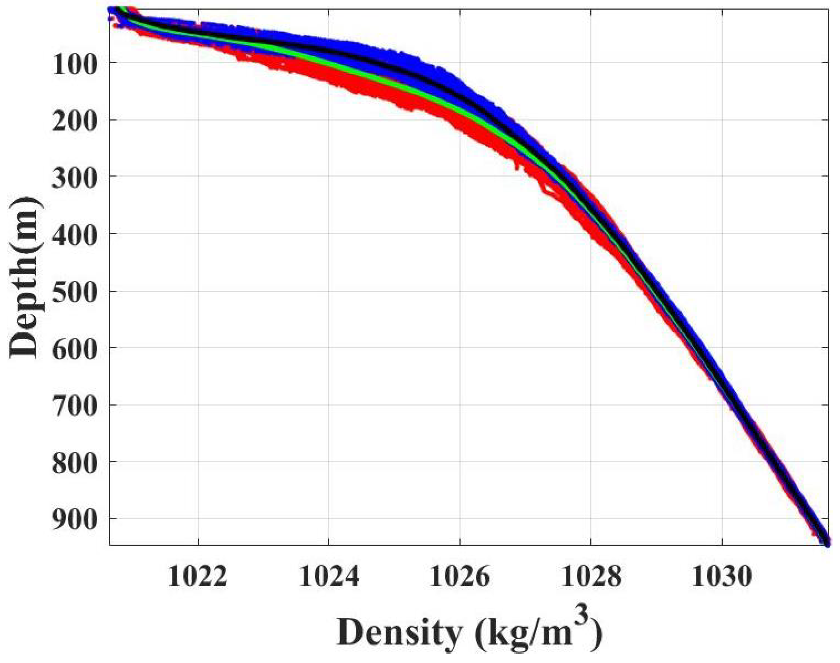
To compare the difference of the density distribution inside and outside the eddy, the whole navigation of UG 6 is divided into three sections: August 5∼12, 13∼15 and 16∼18. During August 5∼12 and 16∼18, UG 6 worked within the eddy; thus, the data collected revealed the density distribution within the eddy. To present the relationship between the density within the eddy and the depth, the data during these periods are extracted and plotted in Figure 6 (marked as red dots in Figure 6). UG 6 navigated outside the eddy during August 13∼15, and the collected data showed the density without the eddy (shown as blue dots in Figure 6). In Figure 6, the green and black solid lines represent the mean density variability inside and outside the eddy, respectively. Comparing the density distribution within and without the eddy in Figure 6, it can be found that the density difference is mainly located near 50∼400 m. Within the depth range, the density inside the eddy is smaller than that outside the eddy, and the maximum difference reaches 0.082 kg/m³.

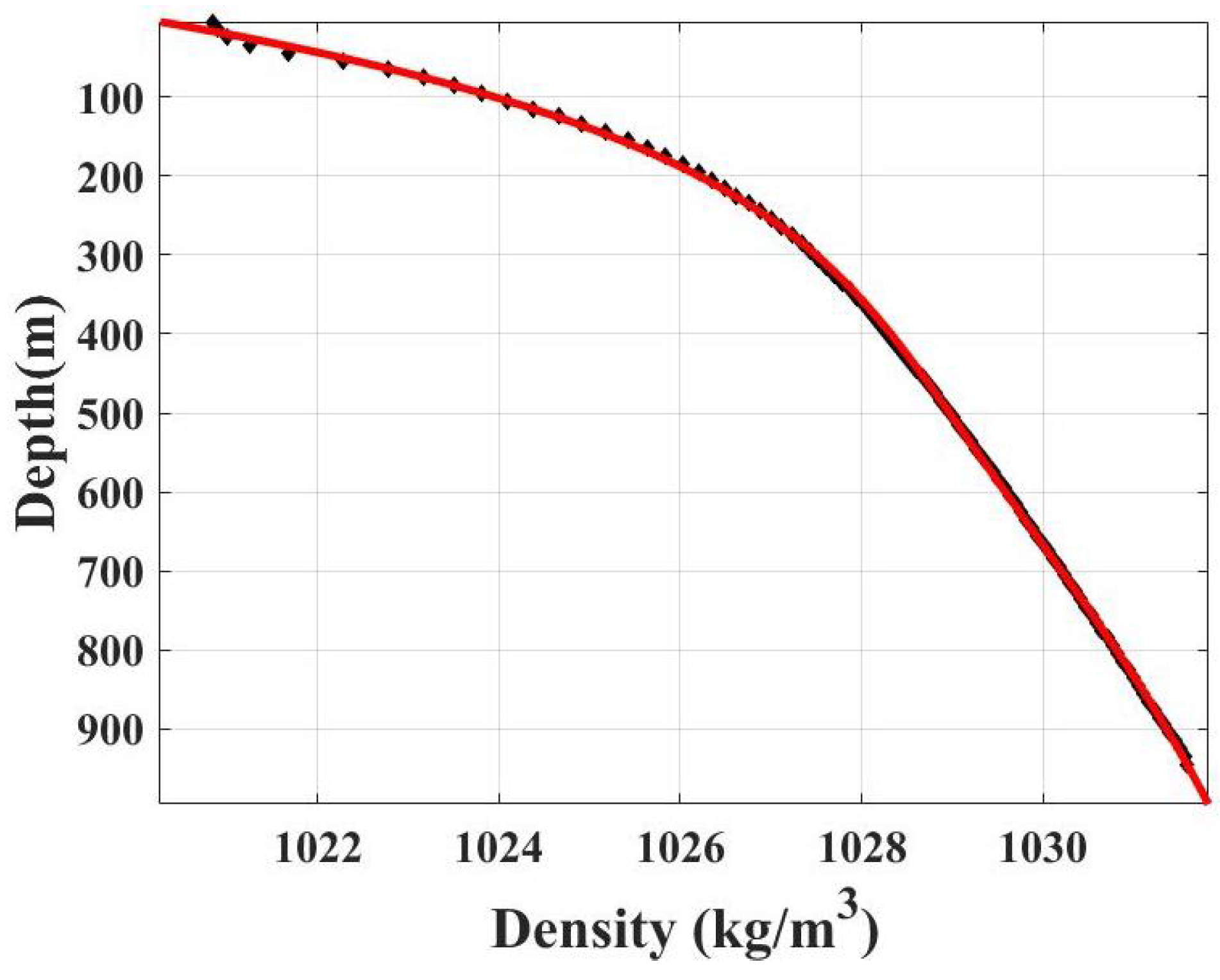
According to the distribution of the mean density within the eddy in Figure 6, a quintic polynomial is adopted to fit the data, and thus, the fitting function between the density and the depth is obtained [35]. The quintic polynomial has the following form. The coefficient of determination (R-square) is 0.9989.

$$\begin{array}{c}{\rho }_{in}\left(h\right)=3.6210\times {10}^{-14}{h}^5-1.3422\times {10}^{-10}{h}^4+1.9152\times {10}^{-7}{h}^3\\ -1.3244\times {10}^{-4}{h}^2+0.0508h+1.0200\times {10}^3\end{array}$$

(5)

where h stands for the depth of the water column (with positive value).

The fitting curve is shown in Figure 7, where the black square represents the mean value of the density within the eddy, and the solid red solid line means the quintic polynomial fitting curve. From Figure 7, the quintic polynomial fits the mean density distribution of the mean density within the eddy well.

Similarly, the data outside the eddy are fitted as a quintic polynomial, which is expressed as the following function. The coefficient of determination (R-square) is 0.9978.

$$\begin{array}{c}{\rho }_{out}\left(h\right)=1.3466\times {10}^{-13}{h}^5-3.8763\times {10}^{-10}{h}^4+4.2771\times {10}^{-7}{h}^3\\ -2.2680\times {10}^{-4}{h}^2+0.0646h+1.0199\times {10}^3\end{array}$$

(6)

The pressure hull of “Petrel II” UG is designed as a cylindrical shape in the middle and semi-ellipsoidal shape in the head and tail [43]. During the descent and ascent, the huge seawater pressure acts on the pressure hull, resulting in the compression deformation of the hull and correspondingly the volume reduction. At a given depth h, the volume of the hull is expressed in the following form [35,38].

$$V\left(h\right)=V_0-\mathsf{\Delta }{V}_h=V_0-kh$$

(7)

where $\mathsf{\Delta }{V}_h$ represents the volume change of the pressure hull and is obtained by pressure test experiment [38]. k means the compression ratio of the pressure hull, k = 0.27172 mL/m.

Equation (4) can be rewritten as Equation (8).

$$B_0=\rho \left(h\right)gV\left(h\right)$$

(8)

where $\rho \left(h\right)$ means the fitting function within the eddy, ${\rho }_{in}\left(h\right)$, or that outside the eddy, ${\rho }_{out}\left(h\right)$.

2.2.2. Other Forces

The gravity of the UG is donated as G, where $G=mg$ and $m=m_m+m_b+m_p$, and the position vector from the mass center to the origin of the body frame is represented as $r_G={[l_{xG},l_{yG},l_{zG}]}^T$. Additional buoyancy generated by the buoyancy adjustment module is expressed as $\mathsf{\Delta }B$, pointing downward in the inertial frame, and its position vector is donated as $r_b={[l_b,0,0]}^T$ in the body frame. The additional buoyancy has the form of

$$\mathsf{\Delta }B=\rho \left(h\right)g\mathsf{\Delta }V$$

(9)

where $\rho \left(h\right)$ is the same as that in Equation (8), and $\mathsf{\Delta }V$ denotes the volume change of the UG caused by the flow of oil into or out of the inner tank.

The mass of the attitude adjustment module is expressed as $m_p$, and the position vector is expressed as $r_p={[l_{xp},l_{yp},l_{zp}]}^T$. The fluid force on the UG can be expressed in the following form.

$$F_f=f(u,v,w,p,q,r)+g(\dot{u},\dot{v},\dot{w},\dot{p},\dot{q},\dot{r})$$

(10)

In Equation (10), $f(u,v,w,p,q,r)$ and $g(\dot{u},\dot{v},\dot{w},\dot{p},\dot{q},\dot{r})$ represent the viscous hydrodynamic force and inertial hydrodynamic force, respectively.

In the velocity frame, the viscous hydrodynamic force can be given in the following form.

$$f=\left[\begin{array}{c}-D\\ SF\\ -L\\ M_x\\ M_y\\ M_z\end{array}\right]=\left[\begin{array}{c}-\frac{1}{2}\rho V^{2}A(C_x\left(0\right)+C_x\left(\alpha \right)\alpha )\\ \frac{1}{2}\rho V^{2}A(C_y\left(\beta \right)\beta +C_y\left(p\right)p^{\prime }+C_y\left(r\right)r^{\prime })\\ -\frac{1}{2}\rho V^{2}A(C_z\left(0\right)+C_z\left(\alpha \right)\alpha +C_z\left(q\right)q^{\prime })\\ \frac{1}{2}\rho V^{2}Al(C_{Mx}\left(\beta \right)\beta +C_{Mx}\left(p\right)p^{\prime }+C_{Mx}\left(r\right)r^{\prime })\\ \frac{1}{2}\rho V^{2}Al(C_{My}\left(0\right)+C_{My}\left(\alpha \right)\alpha +C_{My}\left(q\right)q^{\prime })\\ \frac{1}{2}\rho V^{2}Al(C_{Mz}\left(\beta \right)\beta +C_{Mz}\left(p\right)p^{\prime }+C_{Mz}\left(r\right)r^{\prime })\end{array}\right]$$

(11)

where D, L, and $SF$ represent resistance, lift and side force, respectively, $M_x$, $M_y$, and $M_z$ denote roll moment, pitch moment yaw moment, respectively, $\rho$ means the density of seawater, A is the maximum cross-sectional area of the UG and l is the length of the UG. $C_x\left(0\right)$, $C_y\left(\beta \right)$, $C_y\left(p\right)$, $C_y\left(r\right)$, $C_z\left(0\right)$, $C_z\left(\alpha \right)$, $C_z\left(q\right)$, $C_{Mx}\left(\beta \right)$, $C_{Mx}\left(p\right)$, $C_{Mx}\left(r\right)$, $C_{My}\left(0\right)$, $C_{My}\left(\alpha \right)$, $C_{My}\left(q\right)$, $C_{Mz}\left(\beta \right)$, $C_{Mz}\left(p\right)$, and $C_{Mz}\left(r\right)$ denote the viscous hydrodynamic force or moment coefficients related to attack angle, sideslip attack or angular velocity, respectively. $p^{{}^{\prime }}$, $q^{{}^{\prime }}$, $r^{{}^{\prime }}$ is the dimensionless angular velocity, respectively, during which $p^{{}^{\prime }}=pl/V$, $q^{{}^{\prime }}=ql/V$, $r^{{}^{\prime }}=rl/V$.

In the velocity frame, the inertial hydrodynamic force is expressed as follows.

$$Ih=\left[\begin{array}{c}-{\lambda }_{11}\dot{u}\\ -{\lambda }_{22}\dot{v}-{\lambda }_{26}\dot{r}\\ -{\lambda }_{33}\dot{w}-{\lambda }_{35}\dot{q}\\ -{\lambda }_{44}\dot{p}\\ -{\lambda }_{35}\dot{w}-{\lambda }_{55}\dot{q}\\ -{\lambda }_{26}\dot{v}-{\lambda }_{66}\dot{r}\end{array}\right]$$

(12)

where ${\lambda }_{11}$, ${\lambda }_{22}$, and ${\lambda }_{33}$ mean the added mass, ${\lambda }_{44}$, ${\lambda }_{55}$, and ${\lambda }_{66}$ stand for the added momentum, and ${\lambda }_{26}$ and ${\lambda }_{35}$ represent the additional static moment.

2.3. Dynamic Modeling

Based on the rigid body momentum theorem and angular momentum theorem, the 3D dynamic model of UGs is carefully derived. Since the transect observation of the anticyclonic eddy requires the UGs to move steadily in the vertical plane, the motion of UGs in the vertical plane is discussed in detail. To obtain the dynamic model of UGs in the vertical plane, the parameters of $\beta$, v, p, r, $\varphi$, $\psi$, and Y are set to zeros [21]. Then, the dynamic equations of UGs are rewritten in the form of Equations (13) and (14).

$$\left\{\begin{array}{c}\begin{array}{c}(m+{\lambda }_{11})\dot{u}+m{l}_{zG}\dot{q}+mwq=\mathsf{\Delta }Bsin\theta -(B_0-G)sin\theta \\ -Dcos\alpha +Lsin\alpha \end{array}\\ \begin{array}{c}(m+{\lambda }_{33})\dot{u}+{\lambda }_{35}\dot{q}-m{l}_{xG}\dot{q}-muq=\mathsf{\Delta }Bcos\theta -(B_0-G)cos\theta \\ -Dsin\alpha -Lcos\alpha \end{array}\\ \begin{array}{c}(J_y+{\lambda }_{55})\dot{q}+{\lambda }_{35}\dot{w}=-\mathsf{\Delta }B{l}_{b}cos\theta -G(l_{xG}cos\theta -l_{zG}sin\theta )\\ -m_{p}g(l_{xp}cos\theta -l_{zp}sin\theta )+M_y\end{array}\end{array}\right.$$

(13)

$$\left\{\begin{array}{c}\dot{X}=-usin\theta +wcos\theta \\ \dot{Z}=ucos\theta +wsin\theta \\ V=\sqrt{u^2+w^2}\\ \alpha =arctan\left(\frac{w}{u}\right)\end{array}\right.$$

(14)

where $L=1/2\rho V^{2}A(C_z\left(0\right)+C_z\left(\alpha \right)\alpha )$ and $M_y=1/2\rho V^{2}Al(C_{My}\left(0\right)+C_{My}\left(\alpha \right)\alpha )$. The physical and geometric parameters and the hydrodynamic force or moment coefficients of the UG are shown in

Table 1. The physical and geometric parameters of “Petrel II” UG.

Parameters	Value	Parameters	Value
$m_m$	47.2 kg	$J_y$	22.03 kg⋯m2
$m_b$	7.3 kg	$D_{UG}$	0.22 m
$m_p$	16.4 kg	l	2.1 m
${\lambda }_{11}$	2.0 × ${10}^{-4}$ kg	$l_{xG}$	0.0910 m
${\lambda }_{33}$	0.0153 kg	$l_{zG}$	0.0035 m
${\lambda }_{55}$	9.6 × ${10}^{-4}$ kg	$l_b$	0.9510 m
${\lambda }_{35}$	1.1 × ${10}^{-3}$ kg⋯m	$l_{zp}$	0.0160 m

and

Table 2. The hydrodynamic force or moment coefficients of “Petrel II” UG.

Coefficients	Value	Coefficients	Value
$C_x\left(0\right)$	0.4030	$C_x\left(\alpha \right)$	18.844
$C_z\left(0\right)$	−0.0263	$C_z\left(\alpha \right)$	20.0941
$C_{My}\left(0\right)$	0.0032	$C_{My}\left(\alpha \right)$	−1.5280

, during which the hydrodynamic coefficients are estimated by the computational fluid mechanics (CFD) method [6].

2.4. Validation of the Dynamic Model

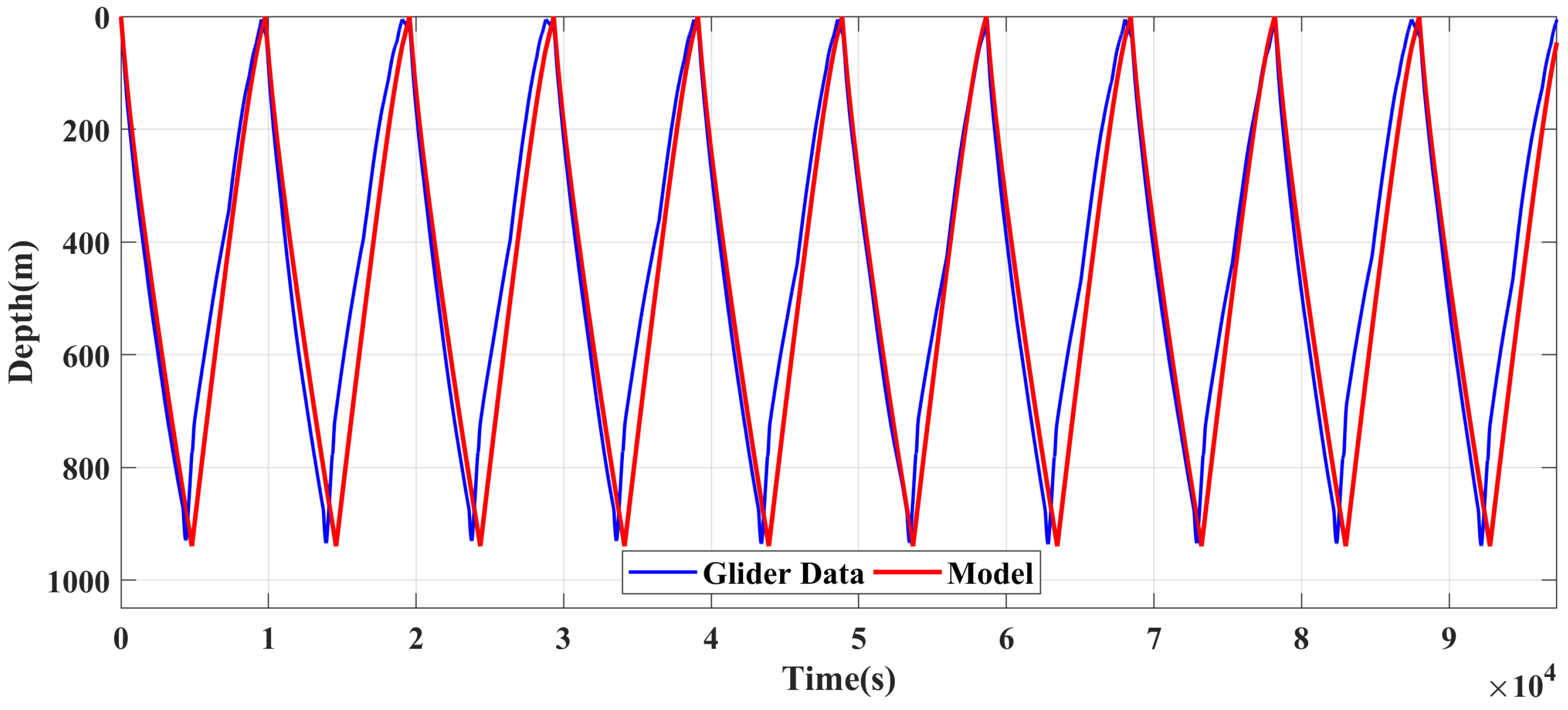
To verify the validity and availability of the established dynamic model considering the effect of the density distribution within the eddy, the in situ data from the field experiments are analyzed to compare with the simulation results. In the simulation, the motion variables of the “Petrel II” UG are obtained by applying the Fourth-Order Runge–Kutta method to solve the dynamic model in the vertical plane expressed by Equations (13) and (14). The initial values of the variables $w_0$, $q_0$, $X_0$, $Z_0$, ${\theta }_0$ are set as zeros, while $u_0$ is set to 0.01 m/s. The proportion of the oil volume in the inner tank and the movement amount of the attitude adjustment module along the Bx-axis and $l_{xp}$ act as input parameters, and these are set to 83%, 17 mm in the descent and 24%, −6 mm in the ascent, respectively. Moreover, the target depth is set to 940 m. During the navigation, UG 6 took transects from August 5∼12 and 16∼18 within the anticyclonic eddy and collected 97 profiles in total. To clearly present the difference between the data from UG 6 and that from the simulations, the data from profiles No. 50∼60 are selected to compare with that from the dynamic model.

Equipped with a SeaBird Glider Payload CTD (described in Section 2.2.1), UG 6 provided the information on the gliding depth along its trajectory, as shown in Figure 8. In Figure 8, the blue and red lines represent the gliding depth obtained from the field experiment and the dynamic model, respectively. Inside the anticyclonic eddy, the vertical velocity is vertically downward in the inertial frame. So, UG 6 descended a little faster in the field experiment than in the simulation during the diving stage. However, the UG ascended slower in the field experiment than in the simulation during the climbing stage. So, the depth difference between the field experiment and simulation is gradually increasing in the descent and reducing in the ascent. Considering that the vertical velocity inside the anticyclonic eddy is about 0.02 m/s at the sea surface and gradually decreases with the increasing depth [44], and the mean vertical velocity of UG is about 0.2 m/s when UG remains stable [42], the effect of the eddy vertical velocity on the motion of UG in the vertical plane is negligible. Assuming that the vertical velocity inside the anticyclonic eddy has a negligible effect on the UG, the gliding depth of UG 6 has a better alignment with that of the model, which means the established dynamic model considering the effect of the density distribution within an eddy has high accuracy in predicting the vertical trajectory of UGs within the eddy. Moreover, the data from the simulations agree better with the experimental data in the descent compared with the ascent, indicating that the dynamic model has a higher prediction accuracy for the descent.

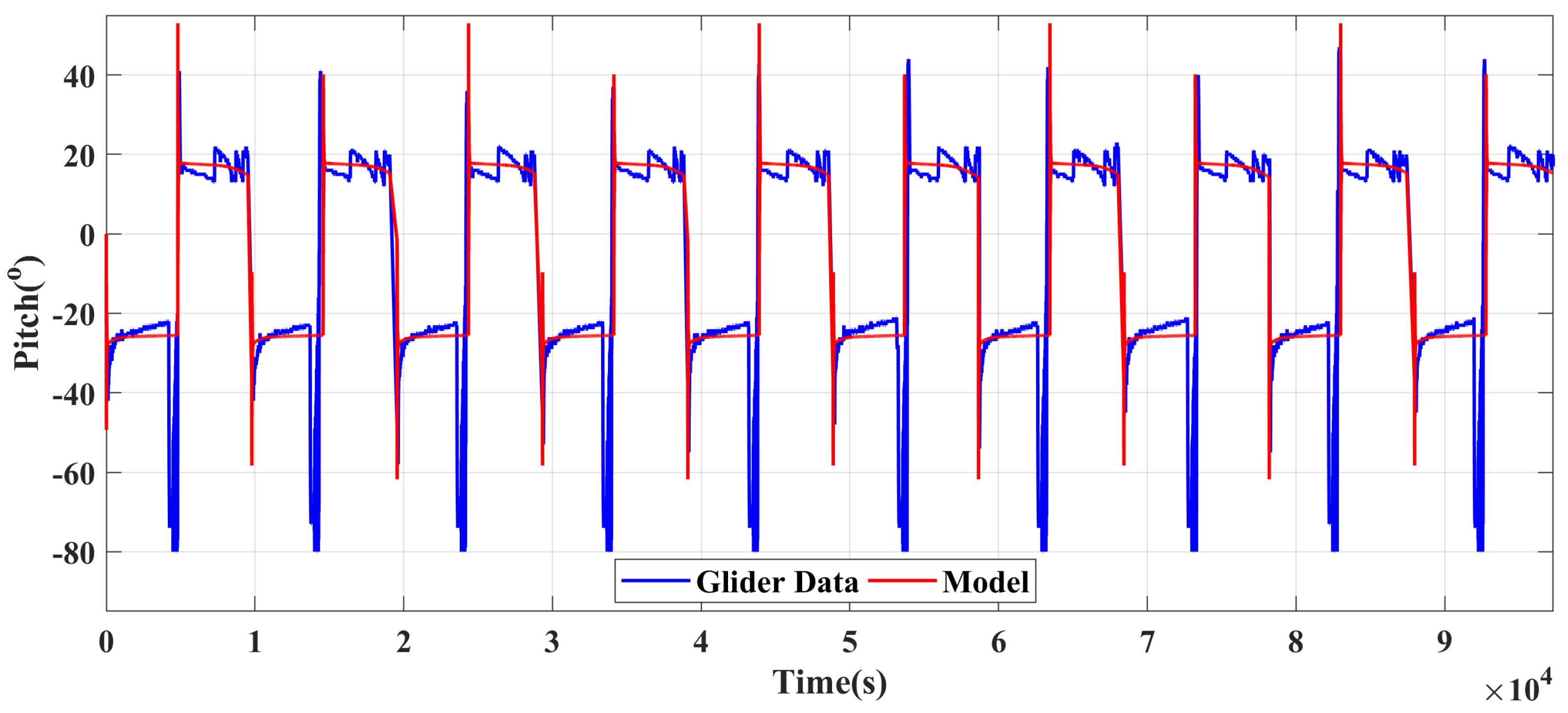
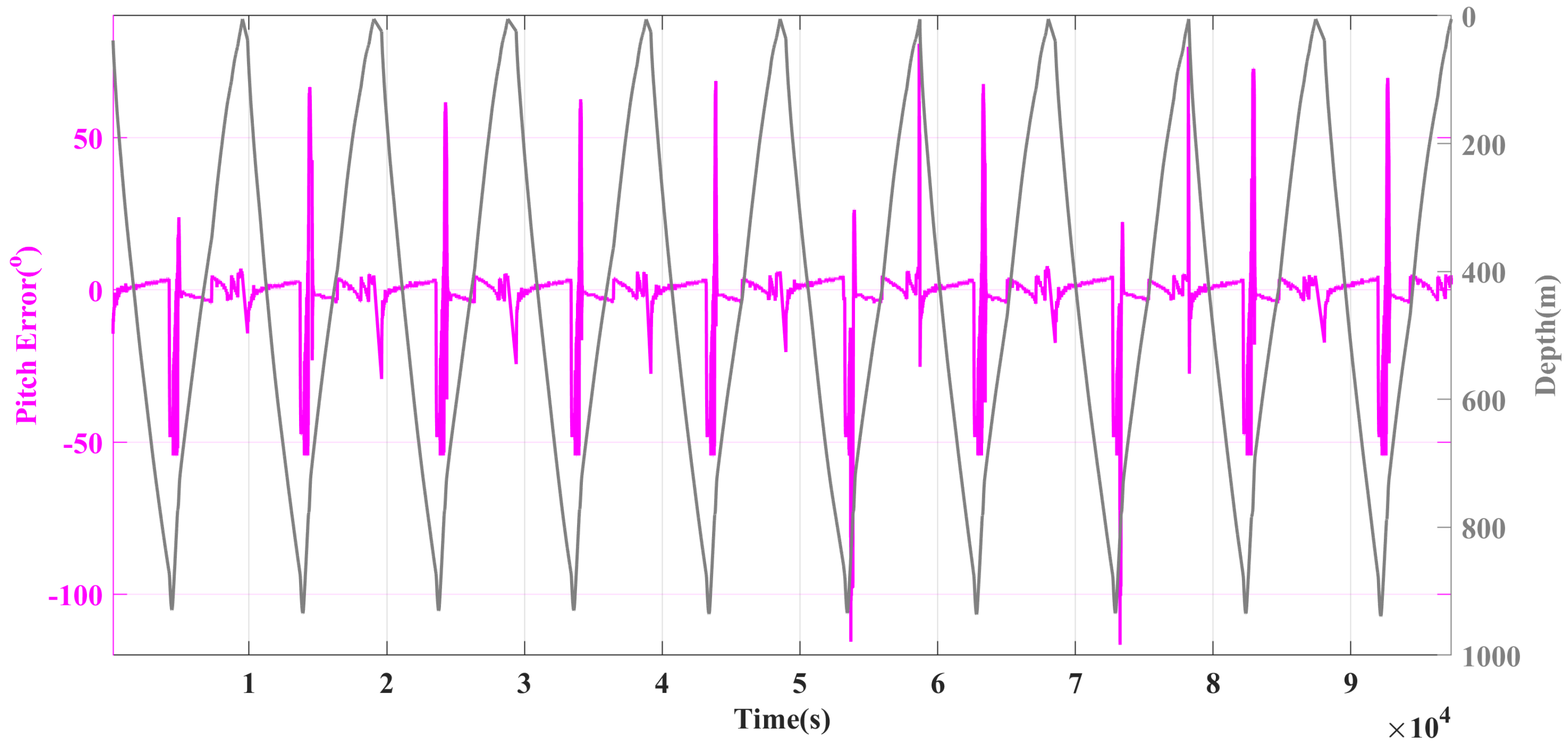
The pitch angle values were acquired by a TCM3 digital compass mounted on UG 6. The pitch angles from UG 6 and the dynamic model are presented in Figure 9. In Figure 9, the trend of the pitch angle derived from UG 6 has considerable similarity to that of the established dynamic model. At the beginning of a profile, UG will adjust its pitch angle and buoyancy to achieve the traveling in a sawtooth trajectory. During the adjustment, the oil flows from the external tank to the inner tank, and the battery in the attitude adjustment model moves forward along the longitudinal axis. Due to the oil flowing inside the UG 6 and the start-up of the oil pump, the errors at a depth of 0∼50 m are shown as peaks in Figure 10. Similarly, during the switching period from the descent to ascent, the peaks occur at a depth of 800∼940 m. After removing the peaks, the mean value of the absolute errors between UG 6 and the model is calculated as 2.1287°, which clarifies the validity of the dynamic model in the analysis of UG attitudes within an eddy in the vertical plane.

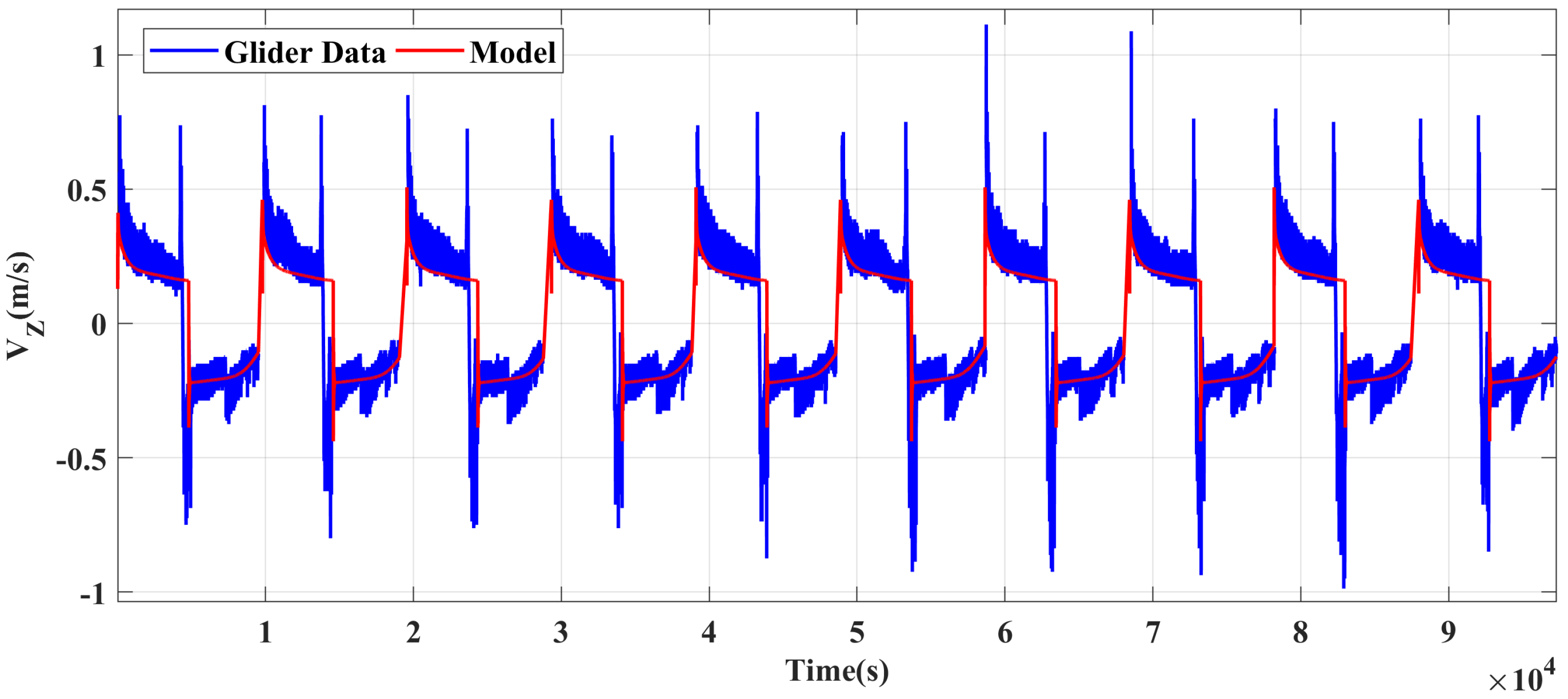
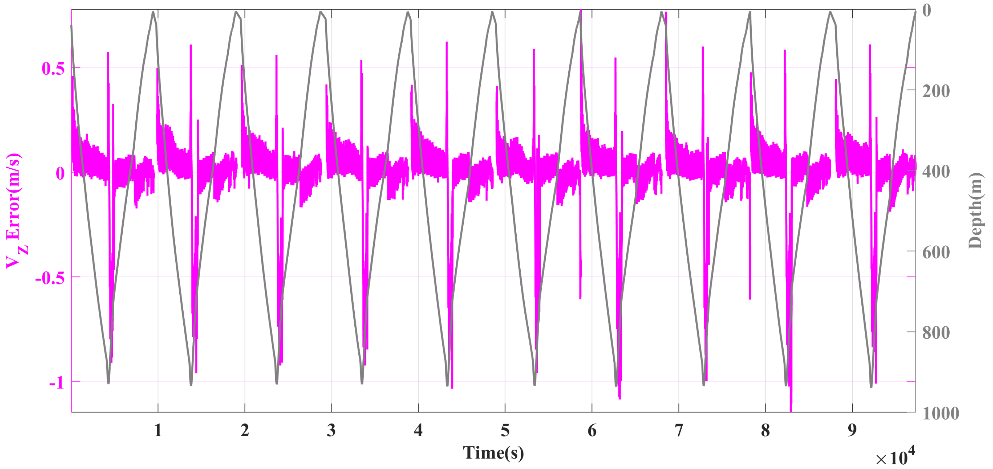
To investigate the motion of UGs within an eddy during the field experiment, the vertical velocity of UG 6 is calculated by the time derivative of depth observed with the pressure sensor [12], as shown in Figure 11. In Figure 11, there exists an obvious consistent pattern in the trend of the vertical velocity between UG 6 and the dynamic model with the smaller values in the deeper water and larger ones in the shallower water during the descent, while the phenomenon is reversed with the larger values in the deeper water and smaller ones in the shallower water during the ascent. To quantify the difference between UG 6 and the model, the errors of the vertical velocity are computed and plotted in Figure 12. Similarly, some peaks during the beginning and the switching period result from the oil flowing inside the UG 6 and the start-up of the oil pump. To calculate the mean error of UG 6 during the stable operation stage, the spikes existing at a depth of 0∼50 m in the descent and 800 m∼940 m in the ascent are removed carefully. Then, the mean value of the absolute errors estimated by UG 6 and the model is 0.0346 m/s, indicating that the dynamic model will be the appropriate choice to analyze the kinematic performance of UGs inside an eddy.

3. Results and Discussion

By considering the variations of the buoyancy, the validity and accuracy of the dynamic model in the vertical plane have been examined in Section 2. In our research, the effect of the density distribution within the anticyclonic eddy on the dynamic behavior of “Petrel II” UG in the vertical plane is discussed thoroughly by analyzing the simulation results of the dynamic model established in Section 2 with the density distribution inside (Model-1) or outside the eddy (Model-2). Same as the simulation setup of Section 2.4, the net buoyancy (calculated by $B_{net}=G-\rho \left(h\right)g(V_h-\mathsf{\Delta }V)$), horizontal velocity, vertical velocity, gliding trajectory and pitch angle of the UG are obtained, as shown in Figure 13, Figure 14, Figure 15 and Figure 16.

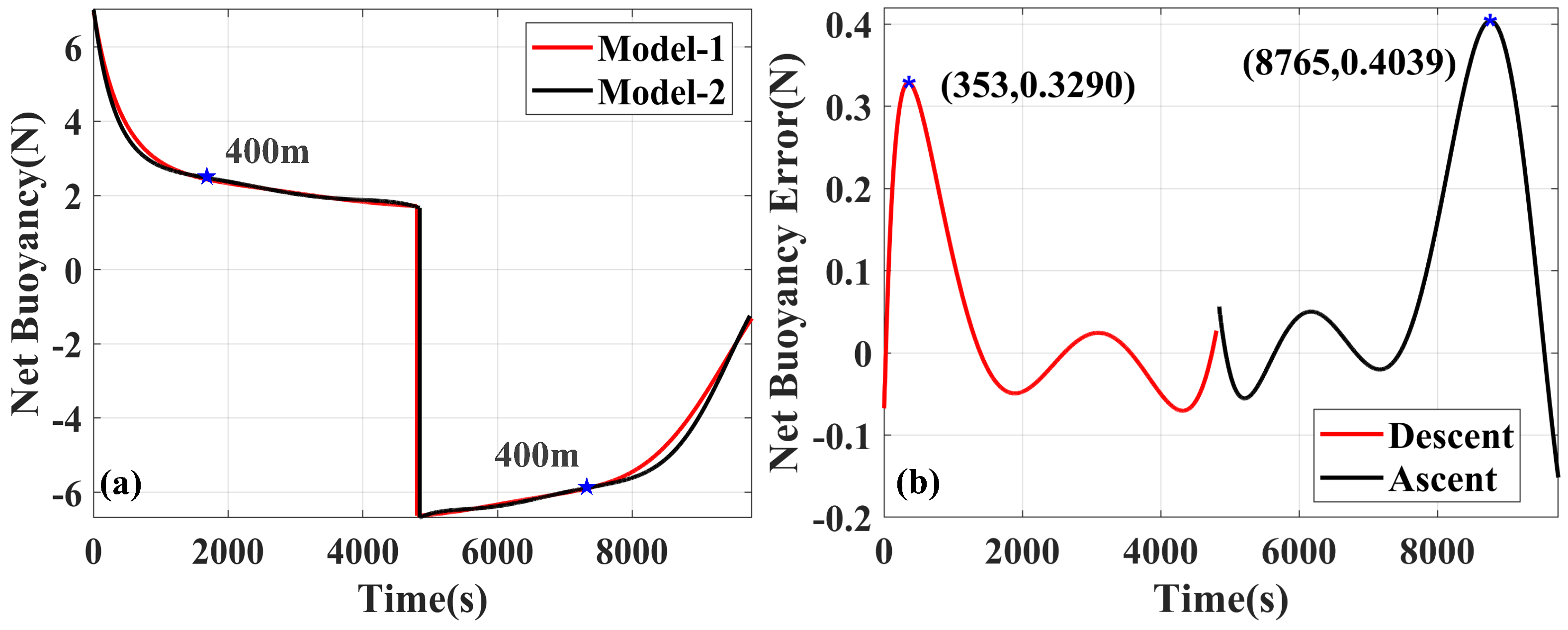
When the movement amount of the attitude adjustment module remains constant, the pitch angle increases with the increasing net buoyancy. It can be seen from Figure 13a that there exists a slight difference in the net buoyancy of Model-1 and Model-2 during the diving (the value less than zero) and climbing (the value greater than zero) stages. The relevant data are listed in

Table 3. Maximums and minimums of net buoyancy and its error in the descent and ascent.

	Descent		Ascent
	Maximum (N)	Minimum (N)	Maximum (N)	Minimum (N)
Model-1	6.9467	1.7168	6.6337	1.3113
Model-2	7.0142	1.6671	6.6844	1.2418
Error	0.3290	−0.0703	0.4039	−0.1515

. The net buoyancy decreases from 6.9467 to 1.7168 N during the descent and from 6.6337 to 1.3113 N during the ascent in Model-1, while in Model-2, it changes from 7.0142 to 1.6671 N and from 6.6844 to 1.2418 N in the descent and ascent, respectively. Obviously, there is a difference of about 0.3 N between the beginning of the descent and ascent both in Model-1 and Model-2, resulting from the compression deformation of the hull and variations of the seawater density. The same phenomenon also occurs at the end of the descending and ascending phases, with a difference of about 0.4 N. In Model-1, the net buoyancy varies dramatically between the sea surface and the depth of about 400 m with an average gradient of about 0.0027 N/m and 0.0019 N/m during the descent and ascent, respectively, while it changes slowly between 400 and 940 m with an average gradient of about 0.0002 N/m and 0.0003 N/m during the descent and ascent, respectively. The errors of the net buoyancy between Model-1 and Model-2 are calculated by subtracting the value of Model-2 from that of Model-1, as shown in Figure 13b. In the descent, the error is within the range of −0.0703 N∼0.3290 N, and the maximum value of the errors reaches up to 0.3290 N at 353 s (about 107 m). Similarly, in the ascent, the value range of the error is [−0.1515 N, 0.4039 N] and the maximum value of the absolute errors achieves 0.4039 N at 8765 s (about 129 m). The results indicate that the larger error of the net buoyancy caused by the eddy density mainly occurs near the depth of the thermocline. Moreover, the estimated mean and standard deviation ($Std$) of the absolute net buoyancy error are 0.0746 N and 0.0916 N, respectively, in the descent. However, they are 0.1150 N and 0.1317 N, respectively, in the ascent, which reveals a stronger influence of eddy density on the net buoyancy of the UG in the ascent than that in the descent.

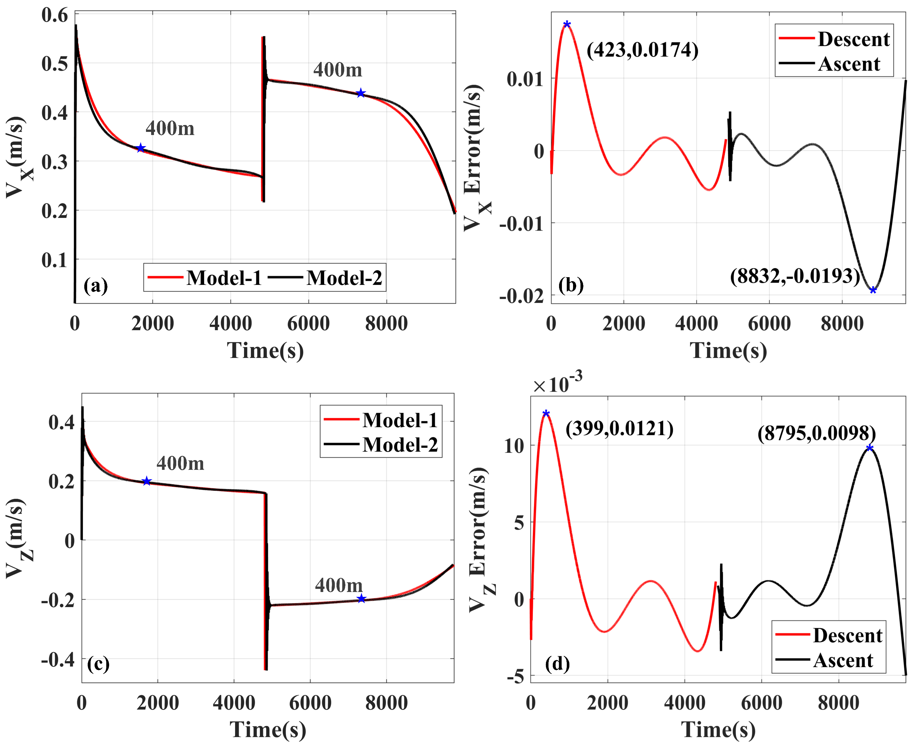
The simulation results of the horizontal ($V_X$) and vertical velocity ($V_Z$) of the UG in the vertical plane are shown in Figure 14a,c and

Table 4. Maximums and minimums of $V_X$ and its errors in the descent and ascent.

	Descent		Ascent
	Maximum (m/s)	Minimum (m/s)	Maximum (m/s)	Minimum (m/s)
Model-1	0.5292	0.2686	0.4666	0.2013
Model-2	0.5784	0.2656	0.4634	0.1916
Error	0.0174	−0.0055	0.0097	−0.0193

and

Table 5. Maximums and minimums of $V_Z$ and its errors in the descent and ascent.

	Descent		Ascent
	Maximum (m/s)	Minimum (m/s)	Maximum (m/s)	Minimum (m/s)
Model-1	0.3312	0.1591	0.2204	0.0876
Model-2	0.3103	0.1569	0.2197	0.0826
Error	0.0121	−0.0034	0.0098	−0.005

. In Model-1, $V_X$ and $V_Z$ in the descent decrease from 0.5292 m/s to 0.2686 m/s and from 0.3312 m/s to 0.1591 m/s, respectively. When switching from the decent to the ascent, both $V_X$ and $V_Z$ change suddenly and fluctuate sharply due to the switch of input parameters, and they decrease from 0.4666 m/s to 0.2013 m/s and from 0.2204 m/s to 0.0876 m/s, respectively, when the UG moves steadily. Both $V_X$ and $V_Z$ vary rapidly from the sea surface to 400 m depth but slowly from 400 to 940 m depth. In the climbing stage, $V_Z$ is larger at 400∼940 m depth with the mean value of 0.2133 m/s than that at a depth of 0∼400 m with the mean value of 0.1648 m/s, while in the diving stage, the variation of $V_Z$ is exactly opposite with $V_Z$ between 400 and 940 m smaller than that between 0 and 400 m. Then, at the same sampling frequency, the vertical sampling resolution of shallow water with a depth less than 400 m is higher than that of deeper water during the climbing of an UG. In the previous work, the vertical structures of temperature, salinity, density, chlorophyll, DO (Dissolved Oxygen) and CDOM (Colored Dissolved Organic Matter) within mesoscale eddies were discussed in detail [4], which revealed that the anomalies within eddies were mainly distributed in the depth of 0∼400 m. To obtain more details of the eddy structure, the climbing profiles are chosen as the available profiles to capture the eddies. Suppose the data are collected in the descent. In that case, it is necessary to increase the sampling frequency of the sensors between the sea surface and 400 m and reduce that from 400 to 940 m to obtain a reasonable vertical sampling resolution. In Model-2, the variation trends of $V_X$ and $V_Z$ are similar to those in Model-1.

To illustrate the differences between the two models in more detail, the errors of $V_X$ and $V_Z$ are represented in Figure 14b,d, respectively. Both positive and negative values of $V_X$ error show a large fluctuation, as seen in Figure 14b. The outliers found between the descent and ascent are caused by switching input parameters and considered as the invalid data. It can be observed that the curve of the $V_X$ error has an approximately centrosymmetric structure and the errors fall in the range of −0.0055 m/s∼0.0174 m/s with the maximum of 0.0174 m/s at 423 s (about 126 m) in the descent and a wider range of −0.0193 m/s∼0.0097 m/s with a larger maximal error of 0.0193 m/s at 8832 s (about 128 m) in the ascent. So, the larger errors appear near 120 m, whether in the descent or the ascent, meaning the greater impact of the eddy density on the horizontal velocity at a depth of about 120 m. For the absolute value of $V_X$ error, the mean and $Std$ values are 0.0045 m/s and 0.0049m/s, respectively, in the descent. However, in the ascent, the mean is 0.0055 m/s, and the standard deviation of 0.0064 m/s, which are both larger than those in the descent. Thus, there is a stronger influence of the eddy density on $V_X$ in the ascent than that in the descent. Different from the variation of $V_X$ error, the error of $V_Z$ shows an approximately axisymmetric structure. In the descent, the fluctuation with the range of −0.0034 m/s∼0.0121 m/s is slightly greater in magnitude than that in the ascent with the range of −0.0050 m/s∼0.0098 m/s. At 399 s (about 120 m) in the descent and 8795 s (about 124 m) in the ascent, there exist two larger peaks of $V_Z$ error, indicating that the eddy density has more influence on the vertical velocity at a depth of about 120 m. To estimate the mean and $Std$, the absolute values of $V_Z$ error are calculated. The mean and $Std$ values are 0.0030 m/s and 0.0034 m/s in the descent, respectively. In the ascent, they are 0.0029 m/s and 0.0036 m/s, respectively. So, there is little difference in the influence of the eddy density on $V_Z$ in the descent and ascent.

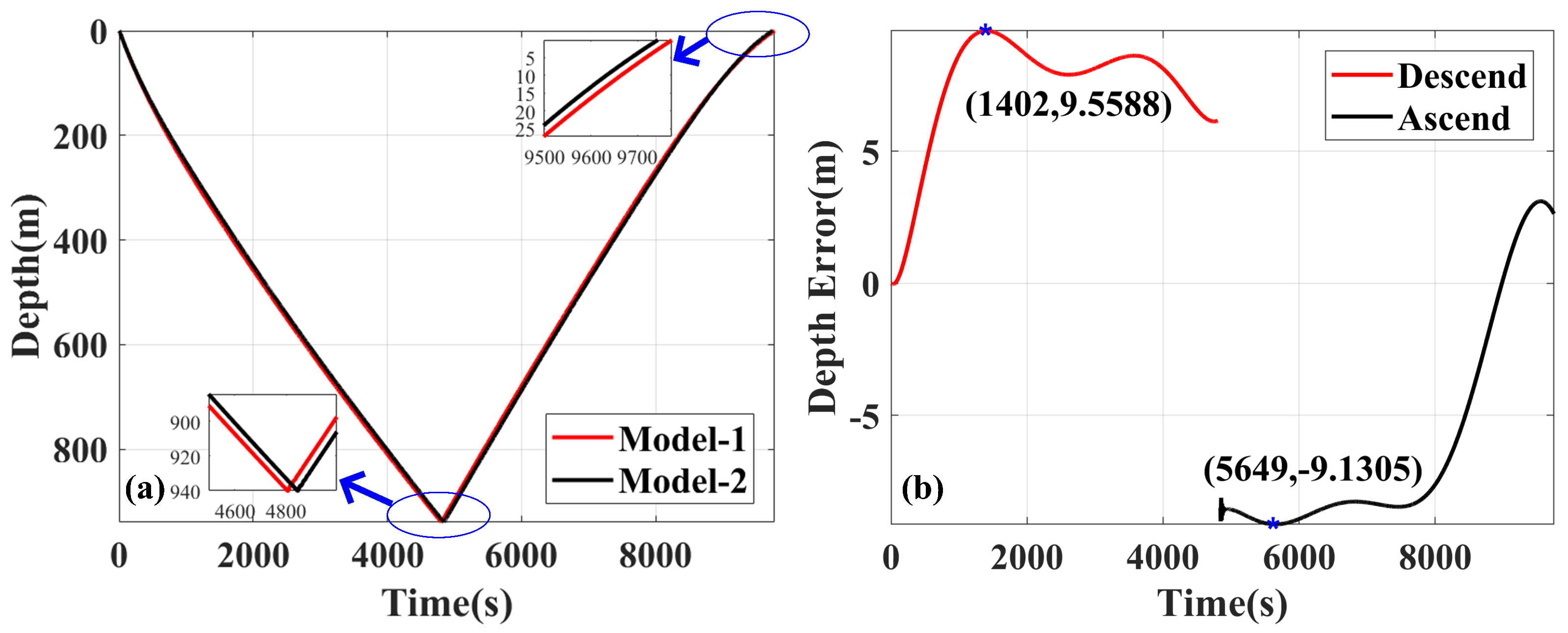
To reveal how the eddy density affects the movement position of the UG, the simulation results of its gliding trajectory and pitch angle are displayed in Figure 15 and Figure 16 and

Table 6. Maximums and minimums of gliding trajectory error in the descent and ascent.

	Maximum (m)	Minimum (m)	Mean	Std	CV
Descent	9.5588	0	7.4059	2.2284	0.3009
Ascent	3.1070	−9.1305	6.7365	2.7849	0.4134

. In Figure 15a, the two trajectories obtained from the simulation using Model-1 and Model-2 almost overlap. However, the time required for an UG to complete a profile simulated based on Model-1 is slightly longer than that based on Model-2, which indicates that the difference of the out-of-water moments simulated by the two models will keep increasing as the number of UG gliding profiles increases. Compared with the simulation results of Model-2, it takes less time for an UG to dive to the specified depth in Model-1 but more time to climb to the sea surface. In order to discuss the trajectory error in more detail, the error between the trajectories simulated by the two models is calculated, as shown in Figure 15b. It can be found that the error fluctuates in both the descent and ascent. In the descent, the error increases gradually from zero to the maximum absolute value of 9.5588 m at 1402 s, when the trajectory obtained from Model-1 reaches 342.6826 m and that obtained from Model-2 achieves 333.1238 m. Then, the error locates at the larger values and fluctuates with a small amplitude, which is consistent with the phenomenon in Figure 14d, where the error of $V_Z$ fluctuates around the value of zero in this stage. In the ascent, the trajectory error reaches the maximum absolute value of 9.1305 m at 5649 s, when the trajectory obtained from Model-1 reaches 755.0830 m, and that obtained from Model-2 reaches 764.2135 m. During the stage of the simulation time larger than 5649 s, the trajectory error also fluctuates near the larger values with a small amplitude and then gradually decreases to zero. Hereafter, it starts to grow in a positive direction because of the $V_Z$ error still being greater than zero. When the error of $V_Z$ is less than zero, the trajectory error starts to decrease. To compare the effect of the eddy density on the trajectory errors in the descent and ascent, the variations of the absolute trajectory error in the two phases are discussed. In the descent, the mean value of the absolute trajectory error is 7.4059 m with the Std value of 2.2284 m, while in the ascent, the mean and $Std$ values are 6.7365 m and 2.7849 m, respectively. Obviously, the mean value in the descent is larger than that in the ascent, but the $Std$ value is smaller. So, the coefficient of variation ($CV$, $CV=Std/mean$ ) is adopted as a normalized index to measure the error dispersion. The $CV$ is calculated to be 0.3009 for the descent and 0.4134 for the ascent, indicating that the trajectory error in the ascent has the larger variability and the trajectory is more influenced by the eddy density, which is consistent with the conclusions discussed above.

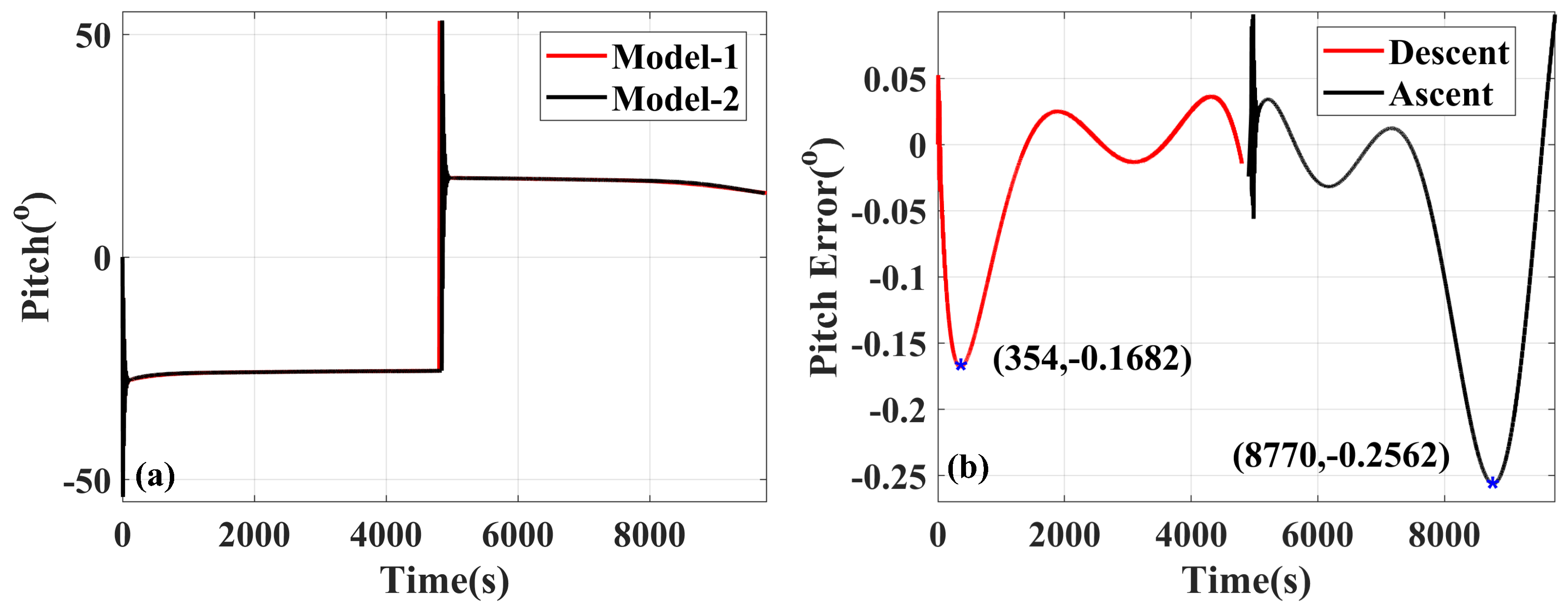
As shown in Figure 16a and

Table 7. Maximums and minimums of pitch angle and its error in the descent and ascent.

	Descent		Ascent
	Maximum (°)	Minimum (°)	Maximum (°)	Minimum (°)
Model-1	27.4562	25.5568	17.7683	14.3615
Model-2	27.3256	25.532	17.7879	14.3175
Error	−0.1682	0.0524	−0.2562	0.0980

, the pitch angle of the UG simulated in Model-1 decreases gradually from 27.4562° to 25.5568° in the descent and from 17.7683° to 14.3615° in the ascent. Similar to the variation in Model-1, the pitch angle obtained from Model-2 also decreases from 27.3256° to 25.5320° in the descent and from 17.7879° to 14.3175° in the ascent. To illustrate the difference in the pitch angle between the two models, the simulation results of the pitch angle error in the vertical plane are shown in Figure 16b. In the descent, the maximum absolute error of 0.1682° occurs at 354 s (about 108 m). Then, the error values fluctuate in a small range. In the ascent, the maximum absolute error of 0.2562° appears at 8770 s (about 128 m). According to the above analysis of the gliding trajectory, the UG simulated in Model-1 reaches the specified depth before Model-2, meaning that the pitch angle in Model-2 keeps the positive value when that in Model-1 switches to the negative value. Therefore, there exists a difference of about 20 m between the depth of the maximum error in the descent and ascent. The mean and Std values of the absolute pitch angle error are 0.0384° and 0.0469°, respectively, in the descent, while these values are 0.0746° and 0.0840°, respectively, in the ascent, both of which are greater than those in the descent, indicating that the mesoscale eddy density makes a stronger effect on the pitch angle of the UG in the ascent.

4. Conclusions

Considering the effect of the density distribution within an eddy on the buoyancy of “Petrel II” UG, the distribution of the eddy density is fitted by a quintic polynomial based on the data collected by a “Petrel II” UG in the sea trial. By combining with the compressibility of the pressure hull, we derive the new expressions of the UG buoyancy which are rewritten as the functions of the water depth h, and thus, the new dynamic model of the UG is established. Assuming there is negligible effect of the vertical velocity inside the anticyclonic eddy on the motion of UG, the analysis of the in situ UG data proves that the established dynamic model has high accuracy in predicting the motion performance of UGs within an eddy in the vertical plane, demonstrating the validity and availability of the dynamic model considering the effect of the density distribution within the eddy to analyze the dynamic behavior of UGs inside an eddy. Based on the established dynamic model, the motion performance of the UG considering the density distribution within the eddy is analyzed.

There is a slight difference in the magnitude of the net buoyance when the dynamic model integrates the density distribution inside an anticyclonic eddy (Model-1) or not (Model-2). In Model-1, there exists a dramatic variation exists from the sea surface to about 400 m depth but a slow variation from about 400 to 940 m depth. The maximum values of the absolute errors between Model-1 and Model-2 reach up to 0.3290 N and 0.4039 N during the descent and ascent, respectively. When the error reaches its maximum values, the depths arrived by the UG simulated with Model-1 are 107 m and 129 m in the descent and ascent, respectively, meaning that the larger error of the net buoyancy caused by the eddy density mainly occurs near the depth of the thermocline. The estimated mean and standard deviation of the absolute net buoyancy are 0.0746 N and 0.0916 N in the descent, respectively, and 0.1150 N and 0.1317 N in the ascent, respectively, indicating that there is a stronger influence of eddy density on the net buoyancy of the UG in the ascent than that in the descent. In Model-1, the value of the horizontal velocity and the vertical velocity in the descent decreases from 0.5292 m/s to 0.2686 m/s and from 0.3312 m/s to 0.1591 m/s, respectively, while in the ascent, they decrease from 0.4666 m/s to 0.2013 m/s and from 0.2204 m/s to 0.0876 m/s, respectively. Similar to the variation of the net buoyancy, both the horizontal velocity and vertical velocity vary rapidly from the sea surface to 400 m depth but slowly from 400 m to 940 m depth. In the ascent, the vertical velocity value is larger at 400∼940 m depth than that at a depth of 0∼400 m. Considering the vertical velocity variations of the UG and the vertical structures of parameters within eddies, the climbing profiles are chosen as the available samples to capture an eddy. If the diving profiles are chosen, increasing the sampling frequency of sensors between the sea surface and 400 m and reducing that from 400 to 940 m will facilitate a reasonable vertical sampling resolution. The curve of the $V_X$ error shows an approximately centrosymmetric structure, and the maximum of the errors is 0.0174 m/s located at about 126 m in the descent and 0.0193 m/s located at about 128 m in the ascent, which means that the larger errors appear near 120 m whether in the descent or the ascent, revealing the greater impact of the eddy density on the horizontal velocity at a depth of about 120 m. In the descent, the mean and standard deviation values of the absolute $V_X$ error are 0.0045 m/s and 0.0049 m/s, respectively. In the ascent, they are 0.0055 m/s and 0.0064 m/s, respectively, which are both larger than those in the descent, showing a stronger influence of the eddy density on $V_X$ in the ascent than that in the descent. When discussing $V_Z$ error, it can be found that there exist two larger peaks of $V_Z$ error at about 120 m in the descent and about 124 m in the ascent, indicating that the eddy density has more influence on the vertical velocity at a depth of about 120 m. Moreover, the mean and standard deviation values are 0.0030 m/s and 0.0034 m/s in the descent, respectively. In the ascent, they are 0.0029 m/s and 0.0036 m/s, respectively, which gives us an important conclusion that there is little difference in the influence of the eddy density on $V_Z$ in the descent and ascent. Moreover, the time required for an UG to complete a profile simulated by Model-1 is slightly longer than that by Model-2. Comparing the simulation results of Model-1 with those of Model-2, it takes less time for an UG to dive to the specified depth in Model-1 but more time to climb to the sea surface. The maximum values of the depth error are located at 9.5588 m and 9.1305 m in the descent and ascent, respectively. The coefficient of variation is calculated to be 0.3009 for the descent and 0.4134 for the ascent, indicating that the trajectory error in the ascent has a larger variability and the eddy density more influences the trajectory. The pitch angle of the UG simulated both in Model-1 and Model-2 decreases gradually both in the descent and ascent. The simulation results of the pitch angle error in the vertical plane show that the maximum error of 0.1682° occurs at about 108 m in the descent and 0.2562° appears at about 128 m in the ascent. In the descent, the mean and standard deviation values of the absolute pitch angle error are 0.0384° and 0.0469°, respectively, while these values are 0.0746° and 0.0840° in the ascent, respectively, both of which are greater than those in the descent, indicating that the mesoscale eddy density makes a stronger effect on the pitch angle in the ascent.

The dynamic model of “Petrel II” UG considering the effect of the density distribution within the eddy contributes to the research on the motion performance analysis of the UG in the complex density distribution within an eddy, which demonstrates that the established dynamic model can predict the movement of the UG in the environment with the complex density distributions. The detailed analysis of the simulation for the dynamic model integrating the density distribution inside an anticyclonic eddy or not shows the differences in the effect of the mesoscale eddy density on the motion performance of “Petrel II” UG in the descent and ascent. Moreover, the results provide a sampling suggestion for applying UGs in the mesoscale eddy observation.

References

- Li, S.; Zhang, F.; Wang, S.; Wang, Y.; Yang, S. Constructing the three-dimensional structure of an anticyclonic eddy with the optimal configuration of an underwater glider network. Appl. Ocean. Res. 2020, 95, 101893. [Google Scholar] [CrossRef]
- Gaube, P.; McGillicuddy, D.J., Jr.; Chelton, D.B.; Behrenfeld, M.J.; Strutton, P.G. Regional variations in the influence of mesoscale eddies on near-surface chlorophyll. J. Geophys. Res. Ocean. 2014, 119, 8195–8220. [Google Scholar] [CrossRef] [Green Version]
- Mcwilliams, J.C.; Liu, Y.; Dong, C.; Chen, D. Global heat and salt transports by eddy movement. Nat. Commun. 2014, 5, 1–6. [Google Scholar]
- Wei, M.; Yanhui, W.; Shuxin, W.; Gege, L.; Shaoqiong, Y. Optimization of hydrodynamic parameters for underwater glider based on the electromagnetic velocity sensor. Proc. Inst. Mech. Eng. J. Mech. Eng. Sci. 2019, 233, 5019–5032. [Google Scholar]
- Nardelli, B.B. Vortex waves and vertical motion in a mesoscale cyclonic eddy. J. Geophys. Res. Ocean. 2013, 118, 5609–5624. [Google Scholar] [CrossRef]
- Mengyao, S. Numerical Simulation of Viscous Hydrodynamics of Unmanned Underwater Glider. Ph.D. Thesis, Tianjin University, Tianjin, China, 2014. [Google Scholar]
- Dickey, T.D.; Itsweire, E.C.; Moline, M.A.; Perry, M.J. Introduction to the Limnology and Oceanography special issue on autonomous and lagrangian platforms and sensors (ALPS). Limnol. Oceanogr. 2008, 53, 2057–2061. [Google Scholar] [CrossRef] [Green Version]
- Yang, M.; Wang, Y.H.; Liang, Y.; Wang, C. A New Approach to System Design Optimization of Underwater Gliders. IEEE/Asme Trans. Mechatronics 2022, 27, 3494–3505. [Google Scholar] [CrossRef]
- Qi, Y.; Shang, C.; Mao, H.; Qiu, C.; Liang, C.; Yu, L.; Yu, J.; Shang, X. Spatial structure of turbulent mixing of an anticyclonic mesoscale eddy in the northern South China Sea. Acta Oceanol. Sin. 2020, 39, 69–81. [Google Scholar] [CrossRef]
- Zhao, J.; Bower, A.; Yang, J.; Lin, X.; Holliday, N.P. Meridional heat transport variability induced by mesoscale processes in the subpolar North Atlantic. Nat. Commun. 2018, 9, 1–9. [Google Scholar] [CrossRef] [Green Version]
- Yu, L.S.; Bosse, A.; Fer, I.; Orvik, K.A.; Bruvik, E.M.; Hessevik, I.; Kvalsund, K. The Lofoten Basin eddy: Three years of evolution as observed by Seagliders. J. Geophys. Res. Ocean. 2017, 122, 6814–6834. [Google Scholar] [CrossRef]
- Martin, J.P.; Lee, C.M.; Eriksen, C.C.; Ladd, C.; Kachel, N.B. Glider observations of kinematics in a Gulf of Alaska eddy. J. Geophys. Res. Ocean. 2009, 114, 1–19. [Google Scholar] [CrossRef] [Green Version]
- Baird, M.E.; Suthers, I.M.; Griffin, D.A.; Hollings, B.; Pattiaratchi, C.; Everett, J.D.; Roughan, M.; Oubelkheir, K.; Doblin, M. The effect of surface flooding on the physical-biogeochemical dynamics of a warm-core eddy off southeast Australia. Deep.-Sea Res. Part II Top. Stud. Oceanogr. 2011, 58, 592–605. [Google Scholar] [CrossRef]
- Cotroneo, Y.; Aulicino, G.; Ruiz, S.; Pascual, A.; Budillon, G.; Fusco, G.; Tintoré, J. Glider and satellite high resolution monitoring of a mesoscale eddy in the algerian basin: Effects on the mixed layer depth and biochemistry. J. Mar. Syst. 2016, 162, 73–88. [Google Scholar] [CrossRef] [Green Version]
- Hodges, B.A.; Fratantoni, D.M. A thin layer of phytoplankton observed in the Philippine Sea with a synthetic moored array of autonomous gliders. J. Geophys. Res. Ocean. 2009, 114, 1–15. [Google Scholar] [CrossRef] [Green Version]
- Thomsen, S. The formation of a subsurface anticyclonic eddy in the Peru-Chile Undercurrent and its impact on the near-coastal salinity, oxygen, and nutrient distributions. J. Geophys. Res. Ocean. 2015, 121, 476–501. [Google Scholar] [CrossRef] [Green Version]
- Yang, G.; Wang, F.; Li, Y.; Lin, P. Mesoscale eddies in the northwestern subtropical Pacific Ocean: Statistical characteristics and three-dimensional structures. J. Geophys. Res. Ocean. 2013, 118, 1906–1925. [Google Scholar] [CrossRef]
- Hu, J.; Gan, J.; Sun, Z.; Zhu, J.; Dai, M. Observed three-dimensional structure of a cold eddy in the southwestern South China Sea. J. Geophys. Res. Ocean. 2011, 116, 1–11. [Google Scholar] [CrossRef] [Green Version]
- He, Q.; Zhan, H.; Cai, S.; He, Y.; Huang, G.; Zhan, W. A New Assessment of Mesoscale Eddies in the South China Sea: Surface Features, Three-Dimensional Structures, and Thermohaline Transports. J. Geophys. Res. Ocean. 2018, 123, 4906–4929. [Google Scholar] [CrossRef]
- Petersen, M.R.; Williams, S.J.; Maltrud, M.E.; Hecht, M.W.; Hamann, B. A three-dimensional eddy census of a high-resolution global ocean simulation. J. Geophys. Res. Ocean. 2013, 118, 1759–1774. [Google Scholar] [CrossRef]
- Leonard, N.E.; Graver, J.G. Model-based feedback control of autonomous underwater gliders. IEEE J. Ocean. Eng. 2001, 26, 633–645. [Google Scholar] [CrossRef] [Green Version]
- Bhatta, P.; Leonard, N.E. Stabilization and coordination of underwater gliders. In Proceedings of the IEEE Conference on Decision and Control, Las Vegas, NV, USA, 10–13 December 2002; Volume 2, pp. 2081–2086. [Google Scholar]
- Graver, J.G. Underwater Gliders: Dynamics, Control and Design. Ph.D. Thesis, Princeton University, Princeton, NY, USA, 2005. [Google Scholar]
- Woolsey, C.A.; Leonard, N.E. Stabilizing underwater vehicle motion using internal rotors. Automatica 2002, 38, 2053–2062. [Google Scholar] [CrossRef]
- Woolsey, C.A.; Leonard, N.E. Moving mass control for underwater vehicles. In Proceedings of the American Control Conference, Anchorage, AK, USA, 8–10 May 2002; Volume 4, pp. 2824–2829. [Google Scholar]
- Mahmoudian, N.; Geisbert, J.; Woolsey, C. Dynamics and Control of Underwater Gliders I: Steady Motions; Technical Report; Virginia Center for Autonomous Systems: Blacksburg, VA, USA, 2009. [Google Scholar]
- Mahmoudian, N.; Woolsey, C.A. An Efficient Motion Control System for Underwater Gliders. Nonlinear Eng. 2013, 2, 63–77. [Google Scholar] [CrossRef]
- Fan, S.; Woolsey, C.A. Dynamics of underwater gliders in currents. Ocean. Eng. 2014, 84, 249–258. [Google Scholar] [CrossRef]
- Arima, M.; Ichihashi, N.; Ikebuchi, T. Motion characteristics of an underwater glider with independently controllable main wings. In Proceedings of the OCEANS 2008—MTS/IEEE Kobe Techno-Ocean, Kobe, Japan, 8–1 April 2008; pp. 1–7. [Google Scholar]
- Arima, M.; Ichihashi, N.; Miwa, Y. Modelling and motion simulation of an underwater glider with independently controllable main wings. In Proceedings of the OCEANS 2009-EUROPE, Bremen, Germany, 11–14 May 2009; pp. 1–6. [Google Scholar]
- Isa, K.; Arshad, M.R.; Ishak, S. A hybrid-driven underwater glider model, hydrodynamics estimation, and an analysis of the motion control. Ocean. Eng. 2014, 81, 111–129. [Google Scholar] [CrossRef]
- Wang, Y. Dynamical Behavior and Robust Control Strategies of the Underwater Gliders. Ph.D. Thesis, Tianjin University, Tianjin, China, 2007. [Google Scholar]
- Wang, S.; Liu, F.; Shao, S.; Wang, Y.; Niu, W.; Wu, Z. Dynamic modeling of hybrid underwater glider based on the theory of differential geometry and sea trails. J. Mech. Eng. 2014, 50, 19–27. [Google Scholar] [CrossRef]
- Zhang, S.; Yu, J.; Zhang, A.; Zhang, F. Spiraling motion of underwater gliders: Modeling, analysis, and experimental results. Ocean. Eng. 2013, 60, 1–13. [Google Scholar] [CrossRef]
- Yang, Y.; Liu, Y.; Wang, Y.; Zhang, H.; Zhang, L. Dynamic modeling and motion control strategy for deep-sea hybrid-driven underwater gliders considering hull deformation and seawater density variation. Ocean. Eng. 2017, 143, 66–78. [Google Scholar] [CrossRef]
- Wang, S.; Li, H.; Wang, Y.; Liu, Y.; Zhang, H.; Yang, S. Dynamic modeling and motion analysis for a dual-buoyancy-driven full ocean depth glider. Ocean. Eng. 2019, 187, 1–11. [Google Scholar] [CrossRef]
- Liu, F.; Wang, Y.H.; Wu, Z.L.; Wang, S.X. Motion analysis and trials of the deep sea hybrid underwater glider Petrel-II. China Ocean. Eng. 2017, 31, 55–62. [Google Scholar] [CrossRef]
- Liu, F. System Design and Motion Behaviors Analysis of the Hybrid Underwater Glider. Ph.D. Thesis, Tianjin University, Tianjin, China, 2014. [Google Scholar]
- Charles, C.E. Autonomous Underwater Gliders. In Underwater Vehicles; IntechOpen Ltd.: London, UK, 2009; pp. 1–5. [Google Scholar]
- Eriksen, C.C.; Osse, T.J.; Light, R.D.; Wen, T.; Lehman, T.W.; Sabin, P.L.; Ballard, J.W.; Chiodi, A.M. Seaglider: A long-range autonomous underwater vehicle for oceanographic research. IEEE J. Ocean. Eng. 2001, 26, 424–436. [Google Scholar] [CrossRef] [Green Version]
- Fofonoff, N.P.; Millard, R.C. Algorithms for computation of fundamental properties of seawater. Unesco Tech. Pap. Mar. Sci. 1983, 44, 53. [Google Scholar]
- Li, S.; Wang, S.; Zhang, F.; Wang, Y. Constructing the three-dimensional structure of an anticyclonic eddy in the South China Sea using multiple underwater gliders. J. Atmos. Ocean. Technol. 2019, 36, 2449–2469. [Google Scholar] [CrossRef]
- Wang, X. Dynamical Behavior and Control Strategies of the Hybrid Autonomous Underwater Vehicle. Ph.D. Thesis, Tianjin University, Tianjin, China, 2009. [Google Scholar]
- Niu, W. Stability Control and Path Planning for Hybrid-driven Underwater Gliders. Ph.D. Thesis, Tianjin University, Tianjin, China, 2016. [Google Scholar]
Figure 1.
The sawtooth trajectory of “Petrel II” UG developed by Tianjin University in the water column.
Figure 2.
(a) The inertial frame and body frame of “Petrel II” UG; (b) The velocity frame of “Petrel II” UG.
Figure 3.
The components of “Petrel II” UG.
Figure 4.
(a) The trajectories of 12 UGs from 4 August 2017 to 29 August 2017 in the South China Sea (the red rectangle highlighted the surveyed domain and the contours on the background represent the isobaths). (b) The trajectory of UG 6 in August 2017 (shown on the SLA map in the domain).
Figure 5.
Seawater density collected by UG 6 in August 2017. The dashed green boxes indicate the transects collected inside the eddy. (a) 0∼900 m (the solid gray box denotes the area shown in (b)). (b) 0∼400 m.
Figure 6.
Comparison of seawater density inside and outside the eddy.
Figure 7.
Fitting curve of seawater density inside the eddy.
Figure 8.
The gliding depth in the vertical plane: UG data vs. simulation results.
Figure 9.
The pitch angle in the vertical plane: UG data vs. simulation results.
Figure 10.
The error of the pitch angle in the vertical plane.
Figure 11.
The vertical velocity in the vertical plane: UG data vs. simulation results.
Figure 12.
The error of the vertical velocity in the vertical plane.
Figure 13.
Simulation results of the net buoyancy and net buoyancy error in the vertical plane. (a) Net buoyancy; (b) Net buoyancy error.
Figure 14.
Simulation results of and in the vertical plane. (a) ; (b) error; (c) ; (d) error.
Figure 15.
Simulation results of the gliding trajectory and its error in the vertical plane. (a) Gliding trajectory; (b) Gliding trajectory error.
Figure 16.
Simulation results of the pitch angle and its error in the vertical plane. (a) Pitch angle; (b) Pitch angle error.