Dynamic Target Tracking of Autonomous Underwater Vehicle Based on Deep Reinforcement Learning

Abstract

Due to the unknown motion model and the complexity of the environment, the problem of target tracking for autonomous underwater vehicles (AUVs) became one of the major difficulties in model-based controllers. Therefore, the target tracking task of AUV is modeled as a Markov decision process (MDP) with unknown state transition probabilities. Based on actor–critic framework and experience replay technique, a model-free reinforcement learning algorithm is proposed to realize the dynamic target tracking of AUVs. In order to improve the performance of the algorithm, an adaptive experience replay scheme is further proposed. Specifically, the proposed algorithm utilizes the experience replay buffer to store and disrupt the samples, so that the time series samples can be used for training the neural network. Then, the sample priority is arranged according to the temporal difference error, while the adaptive parameters are introduced in the sample priority calculation, thus improving the experience replay rules. The results confirm the quick and stable learning of the proposed algorithm, when tracking the dynamic targets in various motion states. Additionally, the results also demonstrate good control performance regarding both stability and computational complexity, thus indicating the effectiveness of the proposed algorithm in target tracking tasks.

1. Introduction

An autonomous underwater vehicle (AUV) is an important tool for exploring the ocean. AUVs possess the ability to complete underwater tasks independently based on the configured sensors and pre-implanted control programs [1,2]. Few underwater tasks require a good target tracking ability, including underwater target reconnaissance, port defense, and underwater docking, etc. [3,4,5,6]. However, during the task execution, the motion of AUV may be easily disturbed by the ocean currents, waves, and other factors [7,8]. Additionally, due to its complex structure, the dynamics of AUVs are nonlinear [9,10]. As a result, the AUV control problem becomes harder to solve.

Most of the methods presented in literature are based on accurate dynamic models for addressing the control problem of AUVs. Prestero et al. [11] established a set of six-degree-of-freedom kinematic and dynamic models based on the REMUS AUV. Assuming that the inclination angle of an AUV is small, the model is linearized, and a proportional-integral-differential controller is designed to control its depth. Refsnes et al. [12] designed a three-degree-of-freedom flow field dynamics model and a five-degree-of-freedom AUV model, combined with the flow field dynamics model, the influence of the seabed flow field on AUVs was accurately described, and an output feedback controller was proposed to control the direction and inclination of the AUV tracking target [13]. All the aforementioned control methods perform well in specific tasks, however, their control performance declines, and an accurate dynamic model is difficult to obtain. Unlike the traditional controllers, the controller obtained using reinforcement learning (RL) does not depend on the accuracy of the model, i.e., it can learn through its interactions with the environment [14,15].

In recent years, the reinforcement learning was developed and successfully applied to the UAV control, autonomous driving and path planning tasks [16,17]. In AUV research, Fakdi et al. [18] used a direct policy search method to learn the strategies for tracking the electric cable, for the state space and action space are discrete. Sun et al. [19] discretized the action space of AUV for target tracking. However, it is noteworthy that poor precision discretization is unable to meet the requirements of control precision, and high precision discretization leads to curse of dimensionality [20].

With the development of deep learning, batch learning, and experience replay techniques [21,22,23], deep reinforcement learning shows an excellent performance in continuous control tasks [24]. Mnih et al. [25] proposed a deep Q-learning (DQN) algorithm, which achieves human level control accuracy in various challenging tasks. However, this method is unable to address the problem of high dimensional state space and high dimensional action space simultaneously [26,27]. Based on the actor–critic framework [28], Lillicrap et al. [20] proposed deep deterministic policy gradient (DDPG) algorithm. This algorithm uses the action network to approximate the deterministic strategy and solves the problem that the DQN algorithm is unable to solve directly in a continuous action space.

When applying the RL algorithms in various tasks, it is critical to establish the corresponding Markov decision process (MDP), including the design of action, state, and reward functions [29]. In complex tasks, the reward function design may involve multiple conflicting control objectives, thus making the task very difficult [30,31]. Therefore, it is necessary to design a reward function that can be used for multiple control objectives. Chowdhury et al. [32] converted the multi-objective problem into a single-objective MDP by scalarizing the one-step rewards with a weight, and completed three simulated mission scenarios to elucidate the approach.

The experience replay technique allows the samples to be used for neural network training [33]. However, in underwater tasks involving AUVs, the battery and storage capacity are limited. As a result, it is impossible to collect samples indefinitely. Moreover, the number of collected samples is generally not enough for appropriately training the model. The original experience replay technique uses the equal probability extraction method to replay the samples, resulting in invalid or low-quality training samples [34]. The temporal difference error reflects the impact of samples on the training process [35]. In order to improve sample utilization, this work considers the temporal difference error based on samples for improving the existing experience replay technique based on the actor–critic algorithm. We propose the adaptive experience replay deterministic policy gradient (AERDPG) for addressing the aforementioned issues.

The main contributions of this work are summarized below.

(1).

We design reward function for multiple control objectives and formulate MDP for the AUV target tracking task.

(2).

The use of the experience replay technique for training leads to low sample utilization. In order to improve the training efficiency, combined with the temporal difference error, an adaptive experience replay rule is proposed.

(3).

Based on the actor–critic algorithm, a reinforcement learning training framework is built, and the target tracking of AUV is realized combined with the experience replay technique.

The rest of this paper is organized as follows: In Section 2, the AUV motion and target tracking are described. In Section 3, the target tracking task is modeled as MDP, and the state, action, and reward functions are designed. In Section 4, an RL algorithm, namely AERDPG, is applied to solve the MDP. In Section 5, the target tracking simulation experiments are performed, and the proposed algorithm is compared with DDPG and PER DDPG algorithms to verify its effectiveness.

2. Problem Formulation

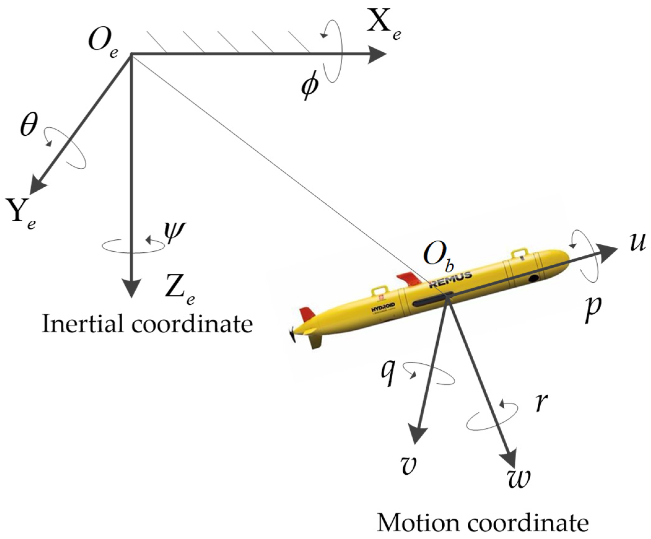
2.1. Coordinate Systems of AUVs

The AUV motion description involves two sets of coordinate systems [36,37], namely the inertial coordinate system and motion coordinate system, as shown in Figure 1, where $\left(\varphi ,\theta ,\psi \right)$ represents the roll angle, pitch angle, and yaw angle of the AUV, respectively, $\left(u,v,w\right)$ denotes the turbulence speed, sway speed, and heave speed, respectively, (p, q, r) denotes the roll angular velocity, pitch angular velocity, and yaw angular velocity, respectively, and $\left(X_e,Y_e,Z_e\right)$ represents the position of the AUV in the inertial coordinate system.

2.2. Dynamic Model of AUVs

The equations of motion of six-DOF AUVs [38] are mathematically expressed as,

$$\{\begin{array}{l}m\left[\dot{u}-vr+wq-x_g\left(q^2+r^2\right)+y_g\left(pq-\dot{r}\right)+z_g\left(pr+\dot{q}\right)\right]=X\\ m\left[\dot{v}-wp+ur-y_g\left(r^2+p^2\right)+z_g\left(qr-\dot{p}\right)+x_g\left(qp+\dot{r}\right)\right]=Y\\ m\left[\dot{w}-uq+vp-z_g\left(p^2+q^2\right)+x_g\left(rp-\dot{q}\right)+y_g\left(rq+\dot{p}\right)\right]=Z\\ I_{xx}\dot{p}+\left(I_{zz}-I_{yy}\right)qr+m\left[y_g\left(\dot{w}-uq+vp\right)-z_g\left(\dot{v}-wp+ur\right)\right]=K\\ I_{yy}\dot{q}+\left(I_{xx}-I_{zz}\right)rp+m\left[z_g\left(\dot{u}-vr+wq\right)-x_g\left(\dot{w}-uq+vp\right)\right]=M\\ I_{zz}\dot{r}+\left(I_{yy}-I_{xx}\right)pq+m\left[x_g\left(\dot{v}-wp+ur\right)-y_g\left(\dot{u}-vr+wq\right)\right]=N\end{array},$$

(1)

where $m$ represents the mass, $I_{xx}$, $I_{yy}$, $I_{zz}$, $I_{xy}$, $I_{xz}$, and $I_{yz}$ represent the moments of inertia of AUVs’ center of gravity relative to its origin, $\left(x_g,y_g,z_g\right)$ represents the center coordinate of AUV, $u$, $v$, $w$, $p$, $q$ and $r$ represent the velocities and angular velocities of AUV, $\dot{u}$, $\dot{v}$, $\dot{w}$, $\dot{p}$, $\dot{q}$ and $\dot{r}$ represent the accelerations and angular accelerations, $X$, $Y$ and $Z$ represent the surge force, sway force, and heave force, respectively, $K$, $M$ and $N$ represent the torques.

The AUV motion is regarded as the sum of the motions in the vertical plane and the surge direction. In this work, the tracking problem is only considered in the vertical plane to simplify the AUV motion. Additionally, the following two common assumptions are made,

(1).

The AUV center of buoyancy coincides with its center of gravity.

(2).

The yaw, pitch, and roll motions can be neglected.

Finally, the AUV motion equation in the vertical plane can be expressed as follows,

$$\begin{array}{l}m\dot{v}=Y_{\left|v\right|v}v\left|v\right|+Y_{\dot{v}}\dot{v}+Y_{uv}uv+Y\\ m\dot{w}=Z_{\left|w\right|w}w\left|w\right|+Z_{\dot{w}}\dot{w}+Z\\ v=v+\dot{v}\Delta t\\ w=w+\dot{w}\Delta t\end{array},$$

(2)

where $Y_{\left|v\right|v}$, $Y_{\dot{v}}$, $Y_{uv}$, $Z_{\left|w\right|w}$ and $Z_{\dot{w}}$ represent the hydrodynamic coefficients and $\Delta d$ is the time interval.

$\tau ={\left[Y,Z\right]}^T$ is the input vector of the AUV, due to the drive limitation, the values of $Y$ and $Z$ have saturated boundaries [9], and they can be expressed as follows,

$$Y=\{\begin{array}{ll}\mathrm{sign}\left(Y\right)Y_M,& \left|Y\right|\ge Y_M\\ Y,& \left|Y\right|<Y_M\end{array},$$

(3)

$$Z=\{\begin{array}{ll}\mathrm{sign}\left(Z\right)Z_M,& \left|Z\right|\ge Z_M\\ Z,& \left|Z\right|<Z_M\end{array},$$

(4)

where $\mathrm{sign}(\cdot )$ represents sign function, $Y_M$ and $Z_M$ represent the saturated boundary of $Y$ and $Z$ respectively. The output vector of AUV is $\eta ={\left[y,z\right]}^T$, which is obtained by the visual sensors. $y$ and $z$ are the relative coordinates of the AUV and the tracked target along the $Y_e$ and $Z_e$ axes in the inertial coordinate system, respectively.

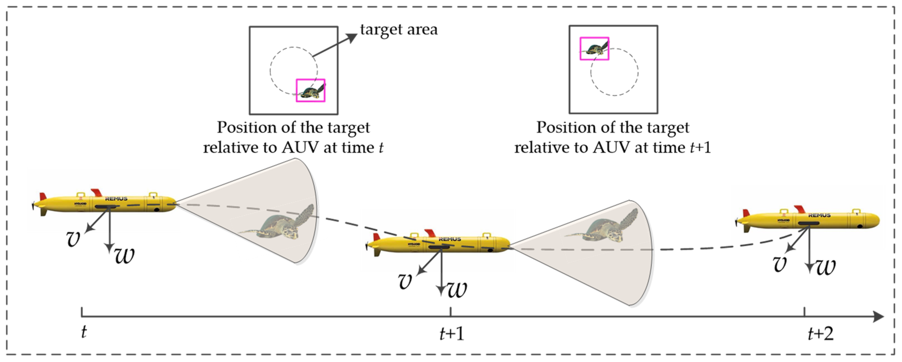
2.3. Target Tracking Tasks

As presented in Figure 2, at time $t$, the target being tracked is located at the bottom right of the AUV. At this time, the AUV is moved to the bottom right, so that the relative position point is returned to the target area. Similarly, the AUV is moved above the left at $t+1$. This is the target tracking process in a unit time period. The continuous time period constitutes the continuous target tracking process of the AUV.

The tracked target motion is time-varying. $p$ is defined as a constant, which represents the probability of the tracked target changing its motion direction and speed. The magnitude of motion change follows normal distribution. Considering the upper and lower limits of motion, the target dynamic equation is mathematically expressed as follows,

$$\{\begin{array}{l}{v}_{obj}=v_{obj}+\varpi n_a\\ d_{obj}=d_{obj}+\varpi n_b\end{array},$$

(5)

$$\varpi =\{\begin{array}{l}0,p_0>p\\ 1,p_0\le p\end{array},$$

(6)

where $\varpi$ denotes the change in the states of tracked target motion, $p_0$ is a randomly generated number between 0 and 1, $n_a\sim N\left(0,a\right)$ and $n_b\sim N\left(0,b\right)$ are the random variables subject to normal distributions, $0\le v_{obj}\le v_{\max }$ is the speed of the target being tracked, and $0\le d_{obj}\le 2\pi$ is the motion direction.

3. MDP of Target Tracking Problem

The goal of MDP is to find a strategy that maximizes the cumulative discount reward, and strategy $\pi$ that maps the states to actions. Therefore, the following optimization objective can be expressed as follows,

$$\underset{\pi \in {\rm P}}{\max }J\left(\pi \right)=\underset{\pi \in {\rm P}}{\max }E\left[{\displaystyle \sum _{t=1}^T{\gamma }^{t-1}{r}_t|\pi }\right],$$

(7)

where $P$ represents the strategy space, $\gamma$ represents the discount factor from 0 to 1, and $T$ represents the maximum step size.

Based on the input vector, the action a_t at $t$ is defined as follows,

$$a_t={\tau }_t={\left[Y_t,{\mathrm{Z}}_t\right]}^T,$$

(8)

in addition, the state $s_t$ is defined by the output vector,

$$s_t={\left[y_{t-1},z_{t-1},y_t,z_t,\sin {\theta }_t,\cos {\theta }_t,v_t\right]}^T,$$

(9)

where $\sin {\theta }_t$ and $\cos {\theta }_t$ jointly describe the relative motion speed directions, and $v_t$ is the relative speed between $t-1$ and $t$, which is expressed as follows,

$$v_t=\frac{\sqrt{{\left(y_t-y_{t-1}\right)}^2+{\left(z_t-z_{t-1}\right)}^2}}{\Delta t}.$$

(10)

Due to the complexity and uncertainty of the underwater environment, the state transition model is defined as a black box function as follows,

$$s_{t+1}=f\left(s_t,a_t,\Delta {\chi }_t\right),$$

(11)

the model shows that, given the state variables and action variables at the current moment, the state variables at the next moment are returned under the interference of noise $\Delta {\chi }_t$.

Target tracking is a multi-objective control problem that includes tracking, stability, and energy saving. First, in order to perform tracking, the AUV motion is controlled to retain the relative motion within the target area. Second, smooth control is achieved by considering the speed of the relative position point entering the target area. Finally, the AUV energy loss during a mission is considered.

During the initial stage of target tracking, there is a distance between the relative position point and the target area. In order to reduce this distance, energy must be consumed to increase the speed of the AUV. In this process, there is a contradiction between the distance from the position point to the target area and the relative speed. In order to mitigate this contradiction between multiple targets during the initial training stage, a variable $\kappa$ related to time is introduced. It is used to measure the effect of objective functions on the training process during different periods. The design reward function is mathematically expressed as follows,

$$r_t=r\left(s_t,a_t\right)=-\left(1-\kappa \right){\rho }_1{\eta }_t{}^T{\eta }_t-\kappa \left({\rho }_2{v}_t+{\rho }_3{a}^{T}a\right),$$

(12)

where ${\rho }_1$, ${\rho }_2$ and ${\rho }_3$ represent the weight coefficients of each item, $-{\rho }_1{\eta }_t{}^T{\eta }_t$ represents the minimal distance between the target location point and the target area, $-{\rho }_2{v}_t$ represents the minimal relative velocity, and $-{\rho }_3{a}^{T}a$ is the minimal consumed energy.

The total reward can be expressed as,

$$R=\sum _{t=1}^T{r}_t,$$

(13)

where $T$ represents the number of time steps.

4. The AERDPG Algorithm

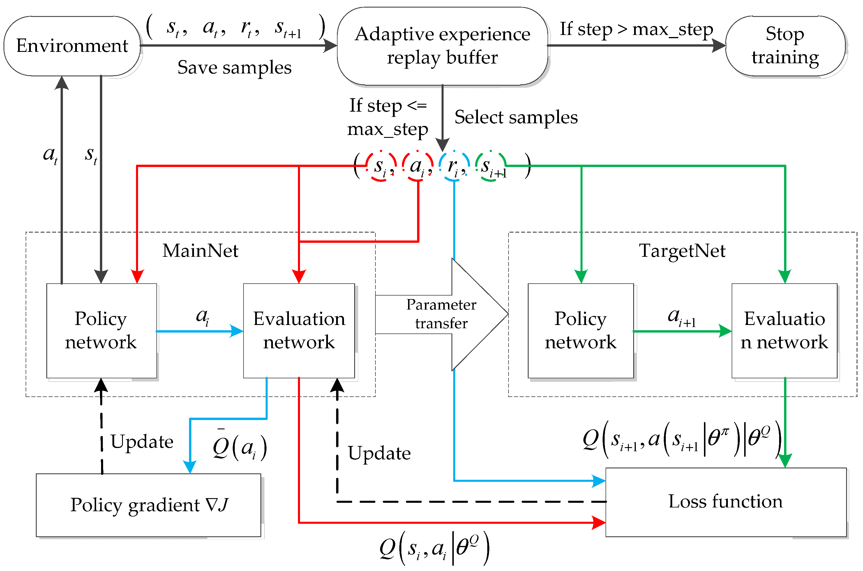
4.1. Algorithm Structure

Based on the actor–critic framework [28], an algorithm denoted as adaptive experience replay deterministic policy gradient (AERDPG) is proposed. The proposed algorithm is developed by using a dual network structure and experience replay technique, as shown in Figure 3.

As presented in Figure 3, the samples generated based on the interaction with the environment are stored in the adaptive experience replay buffer. The data are then selected from the replay buffer as the input of both the main and the target network. In the main network, the evaluation network estimates the function value $Q\left(s_t,a_t|{\theta }^{\pi }\right)$ by applying the temporal difference (TD) method for evaluating both the advantages and disadvantages of the policy network selection action. The evaluation network uses the off-policy method for updating the parameters. The update formula is mathematically expressed as follows,

$$\begin{array}{l}{\delta }_t=r\left(s_t,a_t\right)+\gamma Q\left(s_{t+1},a\left(s_{t+1}|{\theta }^{\pi }\right)|{\theta }^Q\right)-Q\left(s_t,a_t|{\theta }^Q\right)\\ {\theta }_{t+1}^Q={\theta }_t^Q+{\alpha }_Q{\delta }_t{\nabla }_{{\theta }^Q}Q\left(s_t,a_t|{\theta }^Q\right)\end{array},$$

(14)

where ${\alpha }_Q$ is the learning rate of the evaluation network, ${\delta }_t$ is the temporal difference error (TD error), and $a\left(s_{t+1}|{\theta }^{\pi }\right)$ is the output of the policy network, which is responsible for guiding the agent to interact with the environment and update the parameters based on the deterministic policy gradient method [39]. The parameter update formula is expressed as follows,

$${\theta }_{t+1}^{\mu }={\theta }_t^{\mu }+{\alpha }_{\pi }\frac{1}{T}{\displaystyle \sum _{i=1}^T{\nabla }_{{\theta }^{\pi }}a\left(s_i|{\theta }^{\pi }\right){\nabla }_{a_i}Q\left(s_i,a_i|{\theta }^Q\right)},$$

(15)

where ${\alpha }_{\pi }$ denotes the learning rate of the policy network. In the target network, the parameters of each network are transferred by the main network. The output function of the target network is used to construct the loss function.

In order to solve the existing gradient disappearance problem, the neural network uses the ReLU activation function. Then, an adaptive experience replay technique is proposed to improve the sample utilization.

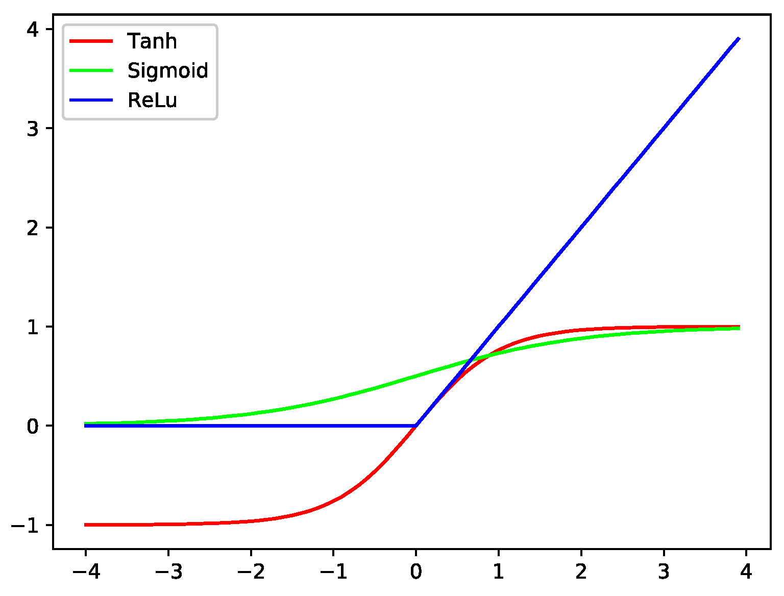
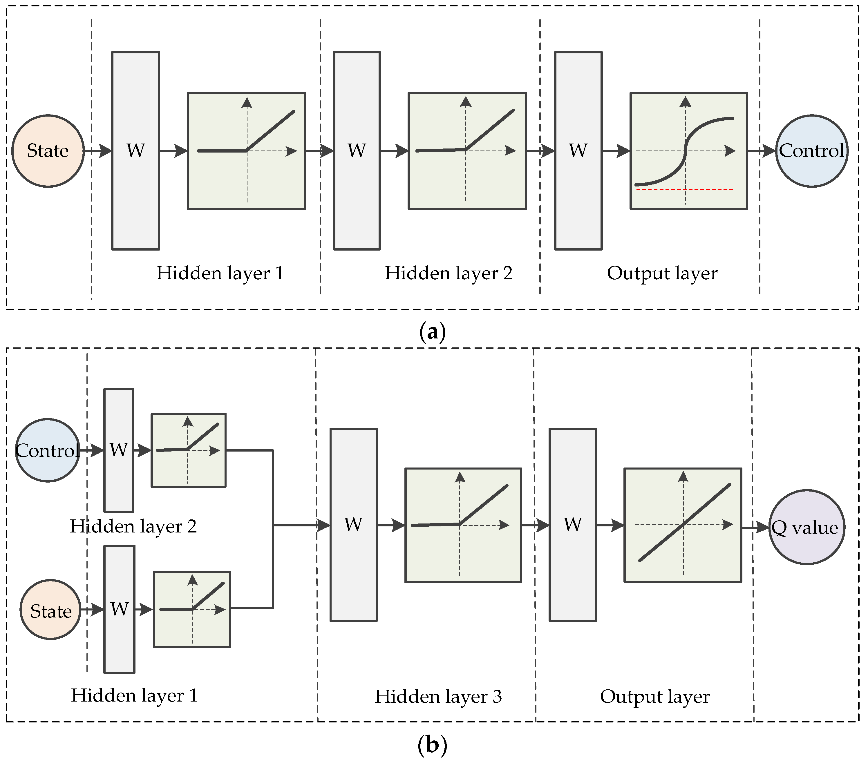
4.2. Neural Network Structure

Considering the nonlinear dynamic characteristics of the AUV, two neural network structures are designed, i.e., the evaluation network and the policy network, with parameters ${\theta }^Q$ and ${\theta }^{\mu }$, respectively.

In the neural network structure, either sigmoid or tanh functions are generally used as the activation functions. These activation functions are very sensitive to the near-zero inputs and insensitive to larger inputs. This saturation property leads to gradient disappearance. In other words, under large input, the element gradient approaches zero, which is not beneficial for network training. The ReLU activation function avoids this problem since it only suppresses the changes in one direction, as shown in Figure 4. Furthermore, the simple ReLU activation function accelerates the network calculation, which is in accordance with the requirements of online tracking.

Therefore, two networks with ReLU activation functions are designed to approximate the strategy function $\mu \left(s|{\theta }^{\mu }\right)$ and value function $Q\left(s,\chi |{\theta }^Q\right)$, as shown in Figure 5. Figure 5a is the policy network structure and Figure 5b is the evaluation network structure.

The policy network has three layers for generating the policies. Its input comprises an amount of state $s_t$ and its output consists of an amount of action $a_t$. The policy network has two hidden layers and an output layer. In order to control the actions within a certain interval, the tanh function is used as the activation function of the output layer. The evaluation network has three layers for evaluating the policy. Its input comprises action $a_t$ and state $s_t$, which pass through two hidden layers, are then combined, and enter in the third implicit layer. Finally, we obtain the value function by using the linear unit of the output layer.

4.3. Adaptive Experience Replay Technique

The experience replay technique eliminates the requirements for independent samples and their identical distribution during the training process of the network. This is done by disrupting the sample order and eliminating the correlation between the samples. Furthermore, the original experience replay technique replays all the samples in the replay buffer with equal probability, and the extracted samples contain a large number of invalid or low-quality individuals. The TD error guides the parameter update of evaluation and strategy networks simultaneously. Additionally, in the experience replay buffer, TD error generated by different samples after entering the evaluation network varies. Therefore, different samples affect the back propagation differently—the greater the TD error, the greater the effect on the network back propagation. The original experience replay technique ignores the difference between the TD errors of the samples, resulting in low sample utilization.

In this work, the sample priority is determined by the absolute sample TD error. The samples with higher priority are considered in subsequent training. The replay probability is defined as follows,

$$P_r\left(i\right)=\frac{\left|{\delta }_i\right|}{{\displaystyle \sum _{i=1}^L\left|{\delta }_i\right|}},$$

(16)

where $L$ denotes the number of samples.

However, during the initial training stage, differences between samples cannot be evaluated properly due to the randomly generated initial parameters of the evaluation network. Thus, the TD error is not accurate, thus making it difficult for samples with a low TD error to be replayed during the initial training stage. As the training process progresses, these samples are replaced by new samples, which degrade the diversity of training samples. Therefore, it is necessary to reduce the impact of TD error on replay probability during the initial training stage. Additionally, the probability of replaying low TD error should be increased to ensure that each sample has a similar replay probability. The probability of replaying samples is mathematically expressed as follows,

$$P\left(i\right)=\mu \times \frac{{\left|{\delta }_i\right|}^{\alpha }}{{\displaystyle \sum _{i=1}^L{\left|{\delta }_i\right|}^{\alpha }}}+b,$$

(17)

where $\alpha$ is a constantly changing value used to adapt to the training process and control the priority degree of the TD error. During the initial training stage $\alpha =0$, the probability of replaying each sample is the same. As the training progresses, $\alpha$ increases until it reaches the maximum value, i.e., $\alpha =1$. The $\mu$ is the normalization coefficient used to ensure that the total sample replay probability is always 1, whereas $b$ is an offset value required to improve the probability of replaying low TD error samples during the whole training process.

4.4. Algorithm Process

Combined with the adaptive experience replay technique and the aforementioned neural network structure, the AERDPG algorithm was proposed. The major steps involved in the proposed algorithm are presented in Algorithm 1.

Algorithm 1. AERDPG for the target tracking of the AUV

Input: number of episodes $M$, number of steps for each episode $T$, batch size $N$, learning rates for evaluation and policy networks ${\alpha }_Q$ and ${\alpha }_{\mu }$, respectively, discount factor $\gamma$, experience replay buffer capacity $L_{\max }$, target motion change probability $p$, and current number of samples in experience replay buffer $L$. Output: Target tracking strategy $a_t=\mu \left(s_t|{\theta }^{\mu }\right)$. 1 Initialize the evaluation network $Q\left(s_t,a_t|{\theta }^Q\right)$ and the policy network $\mu \left(s_t|{\theta }^{\mu }\right)$. Initialize the current number of samples in the experience replay buffer $L$. 2 for $i=1:M$ do: 3  Reset the initial state $s_0$; 4  for $j=1:T$ do: 5   if $R<R_{\max }$: 6    Generate a control strategy $a_t=\mu \left(s_t|{\theta }^{\mu }\right)+\Delta \sigma$ with additional exploration noise $\Delta \sigma$ obtained from the current policy network; 7    Reward $r_{t+1}$ and next state $s_{t+1}$ are obtained from the current state $s_t$ and action $a_t$; 8    Store quadruples $\left[s_t,a_t,r_{t+1},s_{t+1}\right]$ into experience replay buffer; 9   end for; 10   else: 11    The priority of each sample is calculated by Equation (17); 12    Select group $\left[s_t,a_t,r_{t+1},s_{t+1}\right]$ from the experience replay buffer based on $P\left(j\right)$; 13    Update the current evaluation network by Equation (14); 14    Update the current policy network by Equation (15); 15    Transfer the current network parameters to the target network after a pre-defined time step; 16   end for; 17  end for; 18 end for.

5. Experiments

5.1. Experiment Settings

Using the RL algorithm to perform target tracking requires an AUV to explore the environment. Please note that obtaining a large amount of data in the real environment using an AUV is expensive. Therefore, the simulation experiments based on REMUS AUV are performed to obtain the training data. The REMUS AUV was developed and designed by a hydroid company in cooperation with the Naval Research Office. It is one of the widely used AUVs. The specific values of hydrodynamic coefficients [11] are shown in

Table 1. The nonlinear hydrodynamic coefficients of REMUS model AUV.

Coefficient	Value	Coefficient	Value
$m\left(kg\right)$	30.51	$Z_{ww}\left(kg/m\right)$	−131.00
$X_{uu}\left(kg/m\right)$	−1.62	$Z_{\dot{w}}\left(kg\right)$	−35.50
$X_{\dot{u}}\left(kg\right)$	−0.93	$Z_{uw}\left(kg/m\right)$	−28.60

.

For various target motion changing probabilities $p$, the performances of DDPG (based on the original experience replay mechanism) and PER DDPG (based on the priority experience replay mechanism) are compared with the proposed AERDPG algorithm. The number of epochs is set to 2000 and there are 200 steps in each epoch. The learning rates of both the policy and evaluation networks are 0.0005, the hidden layers of policy network is 2, the hidden layers of evaluation networks is 3, the hidden unit is 256, the cumulative reward discount factor is $\gamma =0.99$, the experience replay buffer capacity is 100,000, the batch size is 64, and the soft update parameter is $\tau =0.01$.

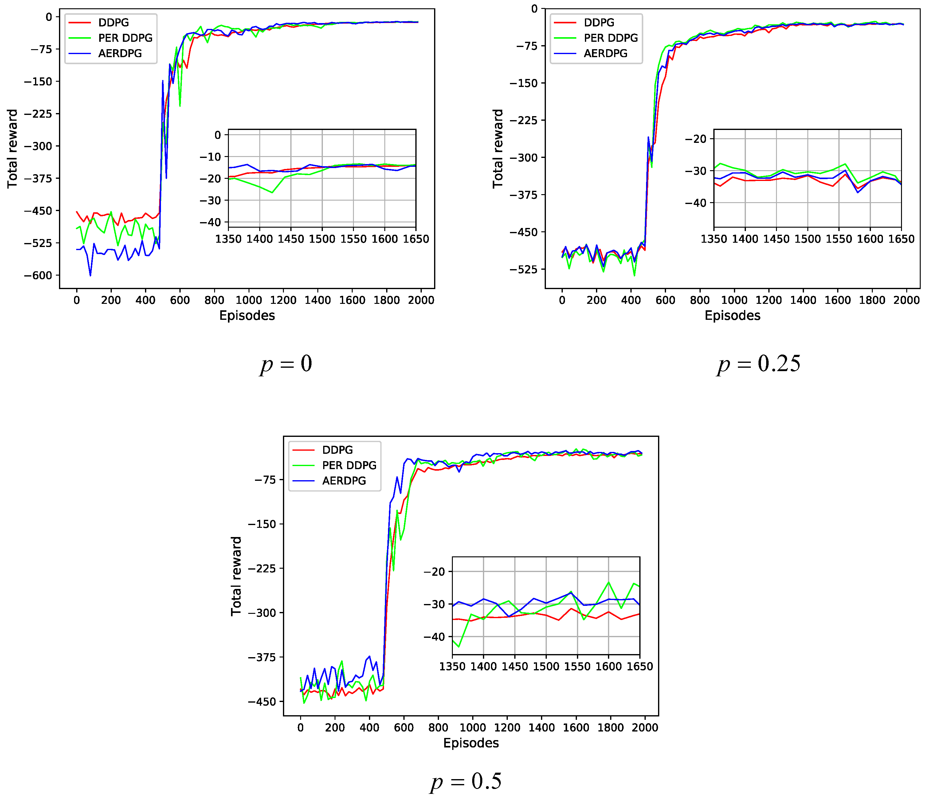
5.2. Training Process Comparison

The training processes for three algorithms are compared and the total reward value curve is obtained, as shown in Figure 6; obviously, no matter what probability, the target changes speed and direction randomly, and the algorithm in this paper can achieve a higher total reward value in 600 episodes, which verifies the feasibility of the algorithm.

Moreover, in order to further compare the performance of the proposed algorithm during the training process, various evaluation indicators are introduced. However, unlike supervised learning, the RL has no separate dataset for training and testing, thus making it difficult to evaluate the online training algorithms. Thus, the sample utilization rate is evaluated by increasing the reward value curve speed. As the time required by the training curve to reach a higher reward value decreases, the curve rises quickly, resulting in a higher sample utilization rate. In addition, the average reward and reward variance are used to evaluate the training stability. The larger the average reward, the smaller the reward variance, indicating that the training process is more stable.

The experiments show that the AUV achieves a better tracking result when the reward value is −40. Therefore, the number of rounds required to reach the reward value −40 is used as the index to evaluate the sample utilization. Moreover, the average reward and its reward variance in both the middle and later training stages are used as the indices to evaluate the training stability. The resulting values are presented in

Table 2. A comparison of experimental results of total reward value.

$p$	Algorithm	DDPG	PER DDPG	AERDPG
$p=0$	Average reward	−18.4416	−18.7932	−16.2437
	Reward variance	41.3573	65.8884	30.8670
	Episodes	732.0000	627.0000	647.0000
$p=0.25$	Average reward	−36.6492	−32.6332	−34.7070
	Reward variance	63.3247	72.3156	53.2815
	Episodes	1021.0000	838.0000	894.0000
$p=0.5$	Average reward	−36.3298	−34.1015	−30.8198
	Reward variance	42.4152	89.9896	70.1450
	Episodes	1032.0000	676.0000	663.0000

* Bold represents the optimal value.

.

By analyzing the aforementioned values, it is evident that the DDPG reward value curve slowly rises, whereas the PER DDPG algorithm performs poorly for the average reward and reward variance. The results imply a certain relationship between the sample utilization and the training sample selection rules. The sample selection affects the training stability during the middle and later stages of the training process. Additionally, the results show that the proposed AERDPG algorithm has advantages in terms of sample utilization and training stability.

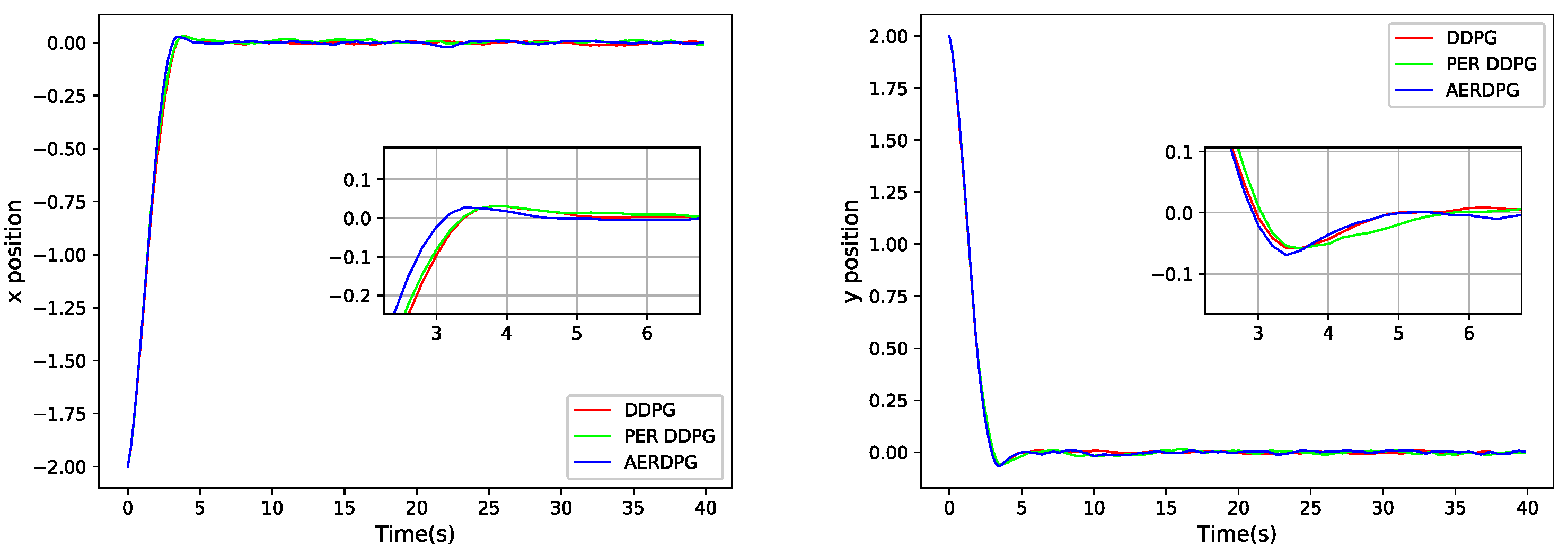
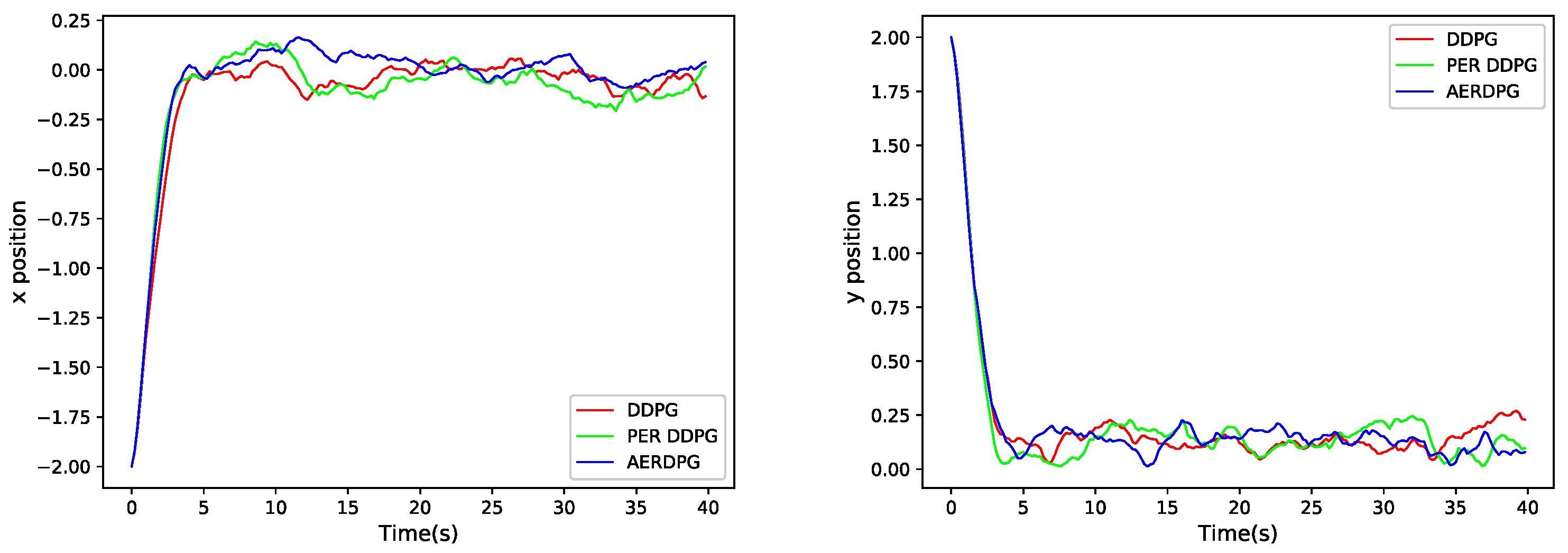
5.3. Controller Performance Comparison

In order to further verify the performance of the control strategy trained by using the proposed AERDPG algorithm, the tracking experiments using the static and dynamic targets are performed. The control performance is evaluated by changing the relative position between the AUV and the target.

First, a static target with the motion changing probability $p=0$ is tracked. The same initial position is set in each experiment to perform the comparison between the experimental results. The initial position is located at the upper left AUV segment and the angle between the connecting line (connecting the target and the center) and the horizontal line is 45 °. As shown in Figure 7, during the initial control stage, the AUV quickly adjusts both the sway and heave force to keep the target in the middle of the relative coordinate system. The relative position in the sway and heave directions approaches zero. However, small amplitude oscillation still occurs due to noise interference.

In order to verify the computational complexity and accuracy of the proposed AERDPG controller, steady-state error, overshoot, and regulation time are observed. The attained values are compared with those values that are obtained by using the DDPG and PER DDPG controllers. It should be noted that the regulation time refers to the time required for the controlled object to reach a steady state. The overshoot denotes the difference between the maximum output value and the steady-state value. On the contrary, the steady-state error denotes the difference between the expected and actual output. The comparison results are shown in

Table 3. The performance indicators of the two controllers (Bold represents the optimal value).

Controller	DDPG	PER DDPG	AERDPG
Sway adjustment time (s)	2.9840	2.9445	2.7473
Sway steady-state error	0.0017	0.0045	0.0026
Sway overshoot	0.0080	0.0171	0.0082
Heave adjustment time (s)	2.6433	2.7214	2.6189
Heave steady-state error	0.0015	0.0019	0.0016
Heave overshoot	0.0105	0.0140	0.0094

.

The numerical analysis shows that the AERDPG and DDPG controllers perform better as compared to the PER DDPG controller in terms of steady-state error, overshoot, and regulation time.

In the next step, a tracking experiment using the dynamic target is conducted with the motion change probability $p=0.25$. The experimental results are shown in Figure 8. During the initial control stage, the controller makes the target reach the central target area quickly. The relative positions in the sway and heave directions approach zero. Due to the randomness of the tracked target motion, the tracking produces oscillations. However, the target is kept in the central area, thus meeting the tracking control requirements.

Due to significant curve oscillations, the performance cannot be evaluated based on the steady-state error, overshoot, and adjustment time. Therefore, the mean relative position and its square deviation are used as the indicators for evaluating the performance. The comparison results are shown in

Table 4. The performance indicators for the three controllers (Bold represents the optimal value).

Controller	DDPG	PER DDPG	AERDPG
Mean value of sway direction	0.0415	0.0792	0.0399
Mean square deviation of sway direction	0.0013	0.0027	0.0012
Mean value in heave direction	0.1282	0.1415	0.1349
Mean square deviation of heave direction	0.0015	0.0026	0.0020

.

The numerical analysis shows that when the motion changing probability of the tracked target is $p=0.25$, the AERDPG and DDPG controllers provide better mean and mean square deviation (of the relative position) results as compared to the PER DDPG controller.

When tracking the static and dynamic targets, the AERDPG controller controls the AUV motion, ensuring that it is always directly behind the target. Its performance is proven to be an improvement with respect to the PER DDPG controller in terms of speed and stability.

6. Conclusions

In this paper, a control method based on deep reinforcement learning is proposed for the AUV target tracking. Considering the time variability in the motion of the target being tracked, the tracked target motion model with different probabilities of motion change is established. The reward function is used to establish the MDP of the corresponding problem. Based on the reinforcement learning actor–critic framework, combined with the timing differential error and adaptive parameters to improve the original experience replay technique, the AERDPG algorithm is proposed. The proposed algorithm combines the determination of strategy gradient and timing differential update neural network, and trains the network with adaptive prioritization samples to improve the utilization of samples. The tracking experimental results of targets with different motion change probabilities confirm the quick and stable learning of the AERDPG algorithm. Additionally, the results also show that the AERDPG algorithm is better as compared to the previous DDPG algorithm in terms of training speed, and the trained controller can track the probability of different motion changes.

References

1. Wang, Y.; Wang, P.; Sun, P. Review on research of control technology of autonomous underwater vehicle. World Sci.-Tech. R & D 2021, 43, 14–26. [Google Scholar]
2. Zhang, Q.; Lin, J.; Sha, Q.; He, B.; Li, G. Deep interactive reinforcement learning for path following of autonomous underwater vehicle. IEEE Access 2020, 8, 24258–24268. [Google Scholar] [CrossRef]
3. Guo, Y.; Qin, H.; Xu, B.; Han, Y.; Fan, Q.-Y.; Zhang, P. Composite learning adaptive sliding mode control for AUV target tracking. Neurocomputing 2019, 351, 180–186. [Google Scholar] [CrossRef]
4. Mintchev, S.; Ranzani, R.; Fabiani, F.; Stefanini, C. Towards docking for small scale underwater robots. Auton. Robot. 2015, 38, 283–299. [Google Scholar] [CrossRef]
5. Li, J.; Li, C.; Chen, T.; Zhang, Y. Improved RRT algorithm for AUV target search in unknown 3D environment. J. Mar. Sci. Eng. 2022, 10, 826. [Google Scholar] [CrossRef]
6. Li, L.; Li, Y.; Zhang, Y.; Xu, G.; Zeng, J.; Feng, X. Formation Control of Multiple Autonomous Underwater Vehicles under Communication Delay, Packet Discreteness and Dropout. J. Mar. Sci. Eng. 2022, 10, 920. [Google Scholar] [CrossRef]
7. Sun, Y.; Ran, X.; Zhang, G.; Wang, X.; Xu, H. AUV path following controlled by modified deep deterministic policy gradient. Ocean. Eng. 2020, 210, 107360. [Google Scholar] [CrossRef]
8. Mannarini, G.; Subramani, D.N.; Lermusiaux, P.F.; Pinardi, N. Graph-search and differential equations for time-optimal vessel route planning in dynamic ocean waves. IEEE Trans. Intell. Transp. Syst. 2019, 21, 3581–3593. [Google Scholar] [CrossRef] [Green Version]
9. Shi, W.; Song, S.; Wu, C.; Chen, C.P. Multi pseudo Q-learning-based deterministic policy gradient for tracking control of autonomous underwater vehicles. IEEE Trans. Neural Netw. Learn. Syst. 2018, 30, 3534–3546. [Google Scholar] [CrossRef] [Green Version]
10. Carlucho, I.; De Paula, M.; Wang, S.; Petillot, Y.; Acosta, G.G. Adaptive low-level control of autonomous underwater vehicles using deep reinforcement learning. Robot. Auton. Syst. 2018, 107, 71–86. [Google Scholar] [CrossRef] [Green Version]
11. Prestero, T. Development of a six-degree of freedom simulation model for the REMUS autonomous underwater vehicle. In Proceedings of the MTS/IEEE Oceans 2001 An Ocean Odyssey. Conference Proceedings (IEEE Cat. No.01CH37295), Honolulu, HI, USA, 5–8 November 2001; Volume 1, pp. 450–455. [Google Scholar]
12. Refsnes, J.E.; Sorensen, A.J.; Pettersen, K.Y. Model-based output feedback control of slender-body underactuated AUVs: Theory and experiments. IEEE Trans. Control. Syst. Technol. 2008, 16, 930–946. [Google Scholar] [CrossRef]
13. Li, D.; Du, L. Auv trajectory tracking models and control strategies: A review. J. Mar. Sci. Eng. 2021, 9, 1020. [Google Scholar] [CrossRef]
14. Carlucho, I.; De Paula, M.; Wang, S.; Menna, B.V.; Petillot, Y.R.; Acosta, G.G. AUV position tracking control using end-to-end deep reinforcement learning. In Proceedings of the OCEANS 2018 MTS/IEEE Charleston, Charleston, SC, USA, 22–25 October 2018; pp. 1–8. [Google Scholar]
15. Mao, Y.; Gao, F.; Zhang, Q.; Yang, Z. An AUV target-tracking method combining imitation learning and deep reinforcement learning. J. Mar. Sci. Eng. 2022, 10, 383. [Google Scholar] [CrossRef]
16. Chowdhury, R.; Subramani, D.N. Physics-driven machine learning for time-optimal path planning in stochastic dynamic flows. In Proceedings of the International Conference on Dynamic Data Driven Application Systems, Boston, MA, USA, 2–4 October 2020; pp. 293–301. [Google Scholar]
17. Bhopale, P.; Kazi, F.; Singh, N. Reinforcement learning based obstacle avoidance for autonomous underwater vehicle. J. Mar. Sci. Appl. 2019, 18, 228–238. [Google Scholar] [CrossRef]
18. El-Fakdi, A.; Carreras, M. Two-step gradient-based reinforcement learning for underwater robotics behavior learning. Robot. Auton. Syst. 2013, 61, 271–282. [Google Scholar] [CrossRef]
19. Sun, T.; He, B.; Nian, R.; Yan, T. Target following for an autonomous underwater vehicle using regularized ELM-based reinforcement learning. In Proceedings of the OCEANS 2015-MTS/IEEE Washington, Washington, DC, USA, 19–22 October 2015; pp. 1–5. [Google Scholar]
20. Lillicrap, T.P.; Hunt, J.J.; Pritzel, A.; Heess, N.; Erez, T.; Tassa, Y.; Silver, D.; Wierstra, D. Continuous control with deep reinforcement learning. arXiv 2015, arXiv:1509.02971. [Google Scholar]
21. Zhao, Y.; Gao, F.; Yu, J.; Yu, X.; Yang, Z. Underwater image mosaic algorithm based on improved image registration. Appl. Sci. 2021, 11, 5986. [Google Scholar] [CrossRef]
22. Hu, K.; Weng, C.; Zhang, Y.; Jin, J.; Xia, Q. An Overview of Underwater Vision Enhancement: From Traditional Methods to Recent Deep Learning. J. Mar. Sci. Eng. 2022, 10, 241. [Google Scholar] [CrossRef]
23. Gao, F.; Wang, K.; Yang, Z.; Wang, Y.; Zhang, Q. Underwater image enhancement based on local contrast correction and multi-scale fusion. J. Mar. Sci. Eng. 2021, 9, 225. [Google Scholar] [CrossRef]
24. Liu, Y.; Swaminathan, A.; Agarwal, A.; Brunskill, E. Provably good batch off-policy reinforcement learning without great exploration. Adv. Neural Inf. Process. Syst. 2020, 33, 1264–1274. [Google Scholar]
25. Mnih, V.; Kavukcuoglu, K.; Silver, D.; Graves, A.; Antonoglou, I.; Wierstra, D.; Riedmiller, M. Playing atari with deep reinforcement learning. arXiv 2013, arXiv:1312.5602. [Google Scholar]
26. Yan, C.; Xiang, X.; Wang, C. Fixed-Wing UAVs flocking in continuous spaces: A deep reinforcement learning approach. Robot. Auton. Syst. 2020, 131, 103594. [Google Scholar] [CrossRef]
27. Devo, A.; Dionigi, A.; Costante, G. Enhancing continuous control of mobile robots for end-to-end visual active tracking. Robot. Auton. Syst. 2021, 142, 103799. [Google Scholar] [CrossRef]
28. Konda, V.R.; Tsitsiklis, J.N. Actor-critic algorithms. In Proceedings of the Advances in Neural Information Processing Systems, Denver, CO, USA, 29 November–4 December 1999; pp. 1008–1014. [Google Scholar]
29. Qin, Z.; Li, N.; Liu, X.; Liu, X.; Tong, Q.; Liu, X. Overview of research on model-free reinforcement learning. Comput. Sci. 2021, 48, 180–187. [Google Scholar]
30. Fechert, R.; Lorenz, A.; Liessner, R.; Bäker, B. Using deep reinforcement learning for hybrid electric vehicle energy management under consideration of dynamic emission models. In Proceedings of the SAE Powertrains, Fuels & Lubricants Meeting, Virtual, Online, Poland, 22–24 September 2020; pp. 2506–2518. [Google Scholar]
31. Chowdhury, R.; Subramani, D. Optimal Path Planning of Autonomous Marine Vehicles in Stochastic Dynamic Ocean Flows using a GPU-Accelerated Algorithm. IEEE J. Ocean. Eng. 2022, 48, 1–16. [Google Scholar] [CrossRef]
32. Chowdhury, R.; Navsalkar, A.; Subramani, D. GPU-Accelerated Multi-Objective Optimal Planning in Stochastic Dynamic Environments. J. Mar. Sci. Eng. 2022, 10, 533. [Google Scholar] [CrossRef]
33. Wu, J.; Wang, R.; Li, R.; Zhang, H.; Hu, X. Multi-critic DDPG method and double experience replay. In Proceedings of the IEEE International Conference on Systems, Man, and Cybernetics, Miyazaki, Japan, 7–10 October 2018; pp. 165–171. [Google Scholar]
34. Ye, Y.; Qiu, D.; Sun, M.; Papadaskalopoulos, D.; Strbac, G. Deep reinforcement learning for strategic bidding in electricity markets. IEEE Trans. Smart Grid 2019, 11, 1343–1355. [Google Scholar] [CrossRef]
35. Hou, Y.; Liu, L.; Wei, Q.; Xu, X.; Chen, C. A novel DDPG method with prioritized experience replay. In Proceedings of the IEEE International Conference on Systems, Man, and Cybernetics, Banff, AB, Canada, 5–8 October 2017; pp. 316–321. [Google Scholar]
36. McCue, L. Handbook of marine craft hydrodynamics and motion control. IEEE Control Syst. Mag. 2016, 36, 78–79. [Google Scholar]
37. Bao, H.; Zhu, H. Modeling and trajectory tracking model predictive control novel method of AUV based on CFD data. Sensors 2022, 22, 4234. [Google Scholar] [CrossRef]
38. Khodayari, M.H.; Balochian, S. Modeling and control of autonomous underwater vehicle (AUV) in heading and depth attitude via self-adaptive fuzzy PID controller. J. Mar. Sci. Technol. 2015, 20, 559–578. [Google Scholar] [CrossRef]
39. Silver, D.; Lever, G.; Heess, N.; Degris, T.; Wierstra, D.; Riedmiller, M. Deterministic policy gradient algorithms. In Proceedings of the International Conference on Machine Learning, Beijing, China, 21–26 June 2014; pp. 387–395. [Google Scholar]
Figure 1. The inertial coordinate system and motion coordinate system of AUV.
Jmse 10 01406 g001
Figure 2. The schematic diagram of AUV dynamic target tracking.
Jmse 10 01406 g002
Figure 3. The flowchart of the proposed algorithm.
Jmse 10 01406 g003
Figure 4. The curves of activation functions.
Jmse 10 01406 g004
Figure 5. The architectures of policy and evaluation networks. (a): the policy network structure; (b): the evaluation network structure.
Jmse 10 01406 g005
Figure 6. The total reward values.
Jmse 10 01406 g006
Figure 7. The AUV control effect for various target motion probabilities.
Jmse 10 01406 g007
Figure 8. The control effect of AUV for various target motion probabilities.
Jmse 10 01406 g008