Robust Optimization Design for Path Planning of Bionic Robotic Fish in the Presence of Ocean Currents

Abstract

The bionic robotic fish is one of the special autonomous underwater vehicles (AUV), whose path planning is crucial for many applications including underwater environment detection, archaeology, pipeline leak detection, and so on. However, the uncertain ocean currents increase the difficulty of path planning for bionic robotic fish in practice. In this paper, the path energy consumption is selected as the objective function for path planning, path safety factor, and smoothness are considered as the constraint conditions. The kinematic model is established for bionic robotic fish and, considering the uncertainty of ocean currents, a “min-max” robust optimization problem is proposed in the light of the normal optimization model of path planning for bionic robotic fish. The co-evolutionary genetic algorithm is presented to solve the robust optimization problem with two populations; one population represents the solutions and the other represents the uncertain ocean currents. The objective of the proposed algorithm is to find a robust solution that has the best worst-case performance over a set of possible ocean currents. Multiple experiments indicate that the proposed algorithm is very effective for path planning for bionic robotic fish with ocean currents.

1. Introduction

As one of the special autonomous underwater vehicles (AUV), the bionic robotic fish has a broad application in the development of marine resources due to its good performance of propulsion efficiency, mobility, and concealment [1,2,3]. In the complex underwater environment, path planning is the key for the bionic robotic fish to arrive at the designated location [4,5]. However, there are many obstacles and uncertain ocean currents in the underwater environment, which increase the difficulty to find an optimal path for improving the path planning performance of the bionic robotic fish.

A lot of research has been conducted based on deterministic methods for solving AUV path planning, including particle swarm optimization (PSO) algorithm, ant colony optimization (ACO) algorithm, A^* algorithm, genetic algorithm, and so on. For shortening path length, reducing travel time, smoothing trajectory and keeping navigation safety, the PSO algorithm is used to obtain the optimal path based on the obstacles detection by a multi-beam forward looking sonars [6]. A multi-objective genetic algorithm is presented for the evaluation of an optimal path and the work gives the designer the freedom to choose one desirable path from a set of Pareto-optimal solutions [7]. An improved quantum particle swarm optimization (IQPSO) algorithm is proposed to satisfy the three factors of path safety, path length, and angle change of the path point [8]. Combining PSO and Legendre pseudo spectral method (LPM), it presents an efficient path-planner based on the hybrid PSO-LPM algorithm to obtain an optimal path with minimum travelling time [9]. In order to find an energy-efficient path, a distance evolution nonlinear PSO algorithm is presented in the three-dimensional underwater acoustic sensor networks [10]; an efficient gain-based dynamic green ACO metaheuristic is proposed to reduce the total energy consumption during path planning [11]; an AUV traversal path is proposed for communication with the underwater wireless sensor networks [12]. To solve the target traveling problem in densely obstructive environments, the ACO-A* algorithm is proposed to obtain an optimal path, ACO is used to determine a traveling order of targets, A* performs pairwise path planning based on a search graph [13]. In order to find the global optimal solution with the shortest path in light of the elite opposition-based learning strategy and the simplex method, an enhanced water wave optimization is used to solve the optimization problem [14]. However, there inevitably exists uncertain ocean currents and all the above deterministic methods [6,7,8,9,10,11,12,13,14] are difficult to be used in the environment with ocean currents for path planning directly and effectively.

The uncertain ocean currents exist in the complex underwater environment, which increases the difficulty of the path planning for bionic robotic fish. To realize the AUV path planning with time-varying ocean currents, the velocity synthesis algorithm is used to adjust the moving direction of AUV to counteract the current influence [15,16]. Although the velocity synthesis algorithm can make the designer obtain a non-collision path in theory, it is difficult to realize the real time accurate measurement of the value and direction of time-varying ocean currents in complex environment. Based on the forecast of the ocean currents, a genetic algorithm is proposed for AUV path planning to find a safe path for minimizing the energy consumption in an ocean environment characterized by strong currents [17]. A quantum particle swarm optimization (QPSO) algorithm is proposed to solve the AUV path planning problem in ocean currents environment [18]. It assumes that the currents remain static in direction and strength over the course of the mission, however, the strong uncertain ocean current or dynamic flow not only reduces the path planning performance index, but even leads the AUV to collide with the obstacles. Recently, fundamental level-set Partial Differential Equations (PDEs) have been developed for AUV time-optimal [19,20,21] and energy-optimal [22,23] path planning in strong and dynamic ocean currents. It can directly utilize a forecast of the dynamic environment to plan collision-free optimal paths that intelligently utilize favorable flows and avoid adverse currents. In these works, the PDEs are used for path planning based on the forecast of the environmental flows, the accuracy of the forecast of the ocean currents determines the effectiveness of the path planning. In summary, in order to obtain an optimal path, the above studies are focused on the forecast of ocean currents [17,19,20,21,22,23], simplifying the ocean currents environments [18] or detecting the currents [15,16] in real time. However, environments simplifying or forecast based on modelling may not match with the real complex underwater environment with strong currents; the ocean current detecting takes up a lot of computing resources and it is difficult to obtain accurate real-time values. Therefore, it needs a new method for path planning for bionic robotic fish in the complex environment with ocean currents.

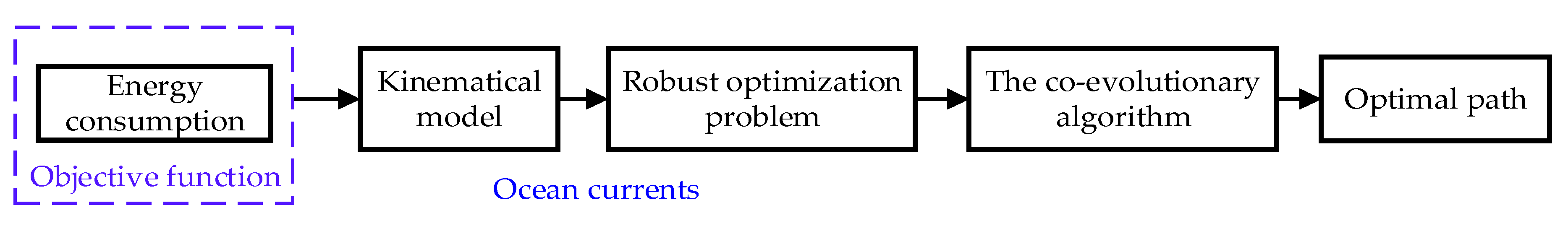
Ocean currents are one of the prominent disturbances for bionic robotic fish in the underwater environment, which can help and hinder the mission for bionic robotic fish [24]. In other words, the bionic robotic fish may save the energy and shorten the path length by allowing it to ride the current, or use more energy and increase the path length through the opposing motion of the ocean forcing. Therefore, the uncertain ocean currents cannot to be ignored for bionic robotic fish path planning in practice. In this paper, in order to solve the path planning for bionic robotic fish with ocean currents, based on the established Kinematic model for bionic robotic fish, an optimization problem is proposed with the objective function of the path energy consumption. Considering the uncertainty of ocean currents, based on the upper and lower limits of ocean currents, it forms a “min-max” robust optimization problem for the path planning for bionic robotic fish, which is solved by the proposed co-evolutionary genetic algorithm. The proposed algorithm can obtain a robust path that has the best worst-case performance over a set of possible ocean currents.

The rest of this paper is organized as follows. Section 2 proposes the problem description of the path planning for bionic robotic fish; Section 3 establishes the mathematical models for the path planning; Section 4 presents the robust optimization problem and the corresponding co-evolutionary genetic algorithm; the simulation results are given and analyzed in Section 5; finally, the paper is concluded in Section 6.

2. Problem Description for the Path Planning

Bionic robotic fish works in the underwater environment, there inevitably exist some obstacles and ocean currents in the complex underwater environment. Ocean currents may lead the bionic robotic fish to deviate from its path, take more time or energy consumption to reach its target point and cause a collision. Therefore, the ocean currents increase the difficulty to obtain an optimal collision-free path for bionic robotic fish. In order to solve the path planning problem for bionic robotic fish easily, some assumptions are given as follows: (1) It ignores the roll motion, because the bionic robotic fish doesn’t easily roll in the underwater environment; (2) The irregular obstacle is represented by a spherical shape that wraps around its contour; and (3) It assumes that the values of ocean currents are in a given range, the range can be obtained based on the historical data. Figure 1 gives the roadmap of path planning for bionic robotic fish in this paper. It selects the path energy consumption as the objective function, combined with the decision variables and constraints in practice, based on the established kinematical model, a deterministic optimization problem is formed for path planning for bionic robotic fish. Considering the ocean currents, a “min-max” optimization problem is proposed for path planning, which is solved by the presented co-evolutionary algorithm; finally, it obtains an optimal path.

3. Mathematical Models for the Path Planning

3.1. Kinematic Model for the Bionic Robotic Fish

Figure 2 gives the workspace of the bionic robotic fish, which includes two coordinate systems of earth-fixed frame $\left\{O-XYZ\right\}$ and body-fixed frame $\left\{O_0-X_0{Y}_0{Z}_0\right\}$. The kinematic model of the bionic robotic fish can be given as follows [25,26,27]:

$$\dot{\mathit{\eta }}=\left[\begin{array}{cc}{\mathit{J}}_1& {\mathbf{0}}_{3\times 3}\\ {\mathbf{0}}_{3\times 3}& {\mathit{J}}_2\end{array}\right]\mathit{V}$$

(1)

$${\left[\begin{array}{cccccc} \dot{x}& \dot{y}& \dot{z}& \dot{\varphi }& \dot{\theta }& \dot{\phi }\end{array}\right]}^T=\left[\begin{array}{cc}{\mathit{J}}_1& {\mathbf{0}}_{3\times 3}\\ {\mathbf{0}}_{3\times 3}& {\mathit{J}}_2\end{array}\right]{\left[\begin{array}{cccccc}u& v& w& p& q& r\end{array}\right]}^T$$

(2)

where $\mathit{\eta }={\left[\begin{array}{cccccc}x& y& z& \varphi & \theta & \psi \end{array}\right]}^T$ is the position and orientation of the bionic robotic fish with respect to the earth-fixed frame, $x$, $y$, $z$ are the position for the bionic robotic fish with respect to the North, East, Down respectively, $\varphi$, $\theta$, $\psi$ are the roll angle, pitch angle, and yaw angle of bionic robotic fish respectively; $\mathit{V}=\left[\begin{array}{cccccc}u& v& w& p& q& r\end{array}\right]$ is the linear and angular velocity vector in the body-fixed frame; $p$, $q$, $r$ are roll rate, pitch rate and yaw rate respectively; $u$, $v$, $w$ are the surge, sway and heave components of velocities respectively; ${\mathit{J}}_1$ and ${\mathit{J}}_2$ are the coordinate transformation matrix relating the two frames respectively, which are expressed as follows:

$${\mathit{J}}_1=\left[\begin{array}{ccc}\cos \psi \cos \theta & -\sin \psi \cos \varphi +\cos \psi \sin \theta \sin \varphi & \sin \psi \sin \varphi +\cos \psi \sin \theta \cos \varphi \\ \sin \psi \cos \theta & \cos \psi \cos \varphi +\sin \psi \sin \theta \sin \varphi & -\cos \psi \sin \varphi +\sin \psi \sin \theta \cos \varphi \\ -\sin \theta & \cos \theta \sin \varphi & \cos \theta \cos \varphi \end{array}\right]$$

(3)

$${\mathit{J}}_2=\left[\begin{array}{ccc}1& \sin \varphi \tan \theta & \cos \varphi \tan \theta \\ 0& \cos \varphi & -\sin \varphi \\ 0& \sin \varphi /\cos \theta & \cos \varphi /\cos \theta \end{array}\right]$$

(4)

In general, the bionic robotic fish do not easily roll in the underwater environment, so it is assumed that $\varphi =0^{\circ }$. In this paper, the Euler angle components of the bionic robotic fish are considered to only be in the XOY plane and the XOZ planes as follows:

$${\psi }_{\mathrm{m}}={\tan }^{-1}\left(\frac{\left|y_{m+1}-y_m\right|}{\left|x_{m+1}-x_m\right|}\right)$$

(5)

$${\theta }_m={\tan }^{-1}\left(\frac{-\left|z_{m+1}-z_m\right|}{\sqrt{{\left(x_{m+1}-x_m\right)}^2+{\left(y_{m+1}-y_m\right)}^2}}\right)$$

(6)

where $\left(x_m, y_m, z_m\right)$ and $\left(x_{m+1}, y_{m+1}, z_{m+1}\right)$ are the two adjacent points on the path.

The components of ocean current vector ($u_c$, $v_c$, $w_c$) in the body-frame is defined as follows:

$$\{\begin{array}{l}{u}_c=\left|{\mathit{V}}_c\right|\cos {\theta }_c\cos {\psi }_c\\ v_c=\left|{\mathit{V}}_c\right|\sin {\theta }_c\cos {\psi }_c\\ w_c=\left|{\mathit{V}}_c\right|\sin {\theta }_c\end{array}$$

(7)

where $\left|{\mathit{V}}_c\right|$ is the magnitude of ocean current velocity ${\mathit{V}}_c$; ${\psi }_c$ and ${\theta }_c$ denote the directions of current in horizontal and vertical planes, respectively. ${\left[\begin{array}{ccc}{u}_c& v_c& w_c\end{array}\right]}^T$ is called the uncertainty of ocean current in this paper.

It assumes that the bionic robotic fish travels with a constant thrust power, in other words, it has a constant water-referenced velocity $\mathit{V}$, then $u$, $v$, $w$ are calculated as follows:

$$\{\begin{array}{l}u=\left|\mathit{V}\right|\cos \varphi \cos \theta +u_c\\ v=\left|\mathit{V}\right|\sin \varphi \cos \theta +v_c\\ w=\left|\mathit{V}\right|\sin \theta +w_c\end{array}$$

(8)

3.2. The Optimization Model for the Path Planning

In the three-dimensional environment, the path energy consumption is crucial for path planning for bionic robotic fish, which determines the endurance time to accomplish the missions for bionic robotic fish [7,8]. Therefore, it selected as the objective function of path planning for bionic robotic fish.

$$\begin{array}{ll}\min & f_E\left(A\right)\\ \mathit{s.t.}& x_{\mathit{min}}\le x_m\le x_{\mathit{max}}\\ & y_{\mathit{min}}\le y_m\le y_{\mathit{max}}\\ & z_{\mathit{min}}\le z_m\le z_{\mathit{max}}\\ & f_S\left(A\right)=1\\ & f_R\left(A\right)=1\\ & \dot{\mathit{\eta }}=\left[\begin{array}{cc}{\mathit{J}}_1& {\mathbf{0}}_{3\times 3}\\ {\mathbf{0}}_{3\times 3}& {\mathit{J}}_2\end{array}\right]\mathit{V}\end{array}$$

(9)

where $x_m$, $y_m$, $z_m$ are the decision variables of the path optimization problem; $A=\left(x_1, y_1, z_1; \cdots ; x_m, y_m, z_m; \cdots ; x_M, y_M, z_M\right)$ are the points on the path, $f_E\left(A\right)$, $f_S\left(A\right)$, $f_R\left(A\right)$ are the path energy consumption, smoothness and safety factor, respectively; $(x_{\mathit{min}},y_{\mathit{min}},z_{\mathit{min}})$ and $(x_{max},y_{max},z_{max})$ are the minimum and maximum coordinate position points, respectively.

It gives the mathematical models of path energy consumption, smoothness, safety factor as follows.

(1) The path energy consumption

In this paper, the path for bionic robotic is made up of the orderly connected points $p_m=\left(x_m, y_m, z_m\right)$, where $m=1,2,\cdots ,M$, $M$ denotes the total number of the path points, the adjacent points are connected by a straight line, the path is given as follows:

$${\Pi }_{s,g}=\langle \overrightarrow{ p_1{p}_2},\overrightarrow{p_2{p}_3},\cdots \overrightarrow{p_{M-1}{p}_M}\rangle$$

(10)

where $p_1$ and $p_M$ are the start and goal path points, respectively.

Based on the distance between two adjacent points in the path of three-dimensional space, the total path length of bionic robotic fish can be given as follows:

$$f_L\left(A\right)={\displaystyle \sum _{m=1}^{M-1}d\left(\overrightarrow{ p_m{p}_{m+1}}\right)}$$

(11)

$$d\left(\overrightarrow{ p_m{p}_{m+1}}\right)=\sqrt{{\left(x_m-x_{m-1}\right)}^2+{\left(y_m-y_{m-1}\right)}^2+{\left(z_m-z_{m-1}\right)}^2}$$

(12)

where $f_L\left(A\right)$ is the total path length; $d\left( \overrightarrow{p_m{p}_{m+1}}\right)$ is the distance between the two adjacent points $p_m$ and $p_{m+1}$.

The energy consumption of path planning for bionic robotic fish is calculated as follows [10,24]:

$$f_E\left(A\right)={\displaystyle \sum _{m=1}^{M-1}{c}_d{v}_m^3{t}_m}={\displaystyle \sum _{m=1}^{M-1}{c}_d{v}_m^3\left(\frac{d\left(\overrightarrow{ p_m{p}_{m+1}}\right)}{\left|\overrightarrow{v_{g,m}}\right|}\right)}$$

(13)

$$\overrightarrow{ v_{g,m}}=\overrightarrow{v_m}+\overrightarrow{V_c}$$

(14)

where $f_E\left(A\right)$ is the path energy consumption, $c_d$ is the bionic robotic fish drag coefficient, $v_m$ is the velocity of the bionic robotic fish; $t_m$ is the travel time for the path $\overrightarrow{p_m{p}_{m+1}}$; $\overrightarrow{ v_{g,m}}$ is the velocity of bionic robotic fish relative to the seabed; $\overrightarrow{V_c}$ is the synthesis of $u_c$, $v_c$, $w_c$ in the path $\overrightarrow{ p_m{p}_{m+1}}$. Equation (13) means the total path energy consumption can be obtained by the sum of the energy consumptions of paths combined by the adjacent points.

(2) The path smoothness

In the process of path planning for bionic robotic fish, the path smoothness should be considered to avoid sudden direction change, the main reasons are given as follows [7]: (1) A sharp change in direction may increase energy consumption and (2) Bionic robotic fish may not be able to track the path with sharp direction changes and pass through unsafe areas. Therefore, the planned path should be gentle and smooth as far as possible. The cosine function has the performance of monotonically decreasing in the interval $\left[0,\pi \right]$, based on the cosine theorem, it can calculate the cosine of the angle between two vectors easily, whose value can be used to calculate the corner angle in this paper. It assumes that the virtual triangle is constituted from the three adjacent points $p_{m-1}$, $p_m$, $p_{m+1}$ (as shown in Figure 3), the cosine function is given to calculate the intersection angle for path planning for bionic robotic fish as follows.

$$\cos \alpha =\frac{b^2+c^2-a^2}{2bc}$$

(15)

$$f_S\left(A\right)=\{\begin{array}{l}1, {\alpha }_{min}<{\alpha }_r<{\alpha }_{max}\\ 0, else\end{array}$$

(16)

where $\alpha$ is the intersection angle with the corner vertex of $p_m$; $\beta$ is the intersection angle with the corner vertex of $p_{m-1}$; $\gamma$ is the intersection angle with the corner vertex of $p_{m+1}$; $a$, $b$, $c$ are the lengths of triangle sides with the corresponding angle of $\alpha$, $\gamma$, $\beta$, respectively; $r=1,2,\cdots ,R$, $R$ is the number of the corner at each turning point; ${\alpha }_r$ is one of the corner angle, which is obtained based on Equation (15). ${\alpha }_{\mathit{min}}$ and ${\alpha }_{\mathit{max}}$ are the minimum and maximum intersection angles respectively, which satisfy $\frac{\pi }{2}<{\alpha }_{\mathit{min}}<{\alpha }_{\mathit{max}}<\pi$.

(3) The path safety factor

The obstacle avoidance is the premise of path planning for bionic robotic fish, which can be evaluated by the safety factor as follows [8].

$$f_R(A)=\{\begin{array}{l}1, d\left(\overrightarrow{ p_m{p}_{m+1}},O_b{}_j\right)>d_0+r_{obs}^j\\ 0, else\end{array}$$

(17)

$$d\left(\overrightarrow{ p_m{p}_{m+1}},O_b{}_j\right)=\frac{\Vert \overrightarrow{p_m{p}_{m+1}}\times \overrightarrow{p_m{O}_{bj}}\Vert }{d\left(\overrightarrow{p_m{p}_{m+1}}\right)}$$

(18)

where $f_R\left(A\right)$ is the safety factor of the path planning for robotic fish; $O_b{}_j$ is the centre of the virtual spherical obstacle, which envelops the actual irregular obstacle; $r_{obs}^j$ is the radius of the $j-th$ spherical obstacle, $j$ is the serial number of the obstacle; $d(\overrightarrow{ p_m{p}_{m+1}},O_b{}_j)$ is the distance between $\overrightarrow{ p_m{p}_{m+1}}$ and $O_b{}_j$; $d_0$ is a positive number. When the line between two adjacent path points does not pass through the obstacle, the value of $f_R\left(A\right)$ is 1, which represents the path safety. Otherwise, the path is danger of colliding with obstacles.

4. Robust Optimization Design for Path Planning

In this paper, the bionic robotic fish works in a complex underwater environment, it is a challenge problem of non-collision path planning with low energy consumption in the presence of ocean currents [16]. Robust optimization is the problem to find the best solution in the worst cases, it’s also called “min-max” problem, which is proposed to solve the path planning with the ocean currents. Considering the uncertain of ocean currents, Equation (9) is transformed into a “min-max” optimization problem as follows.

$$\begin{array}{l}\underset{(x_m,y_m,z_m)}{\min } \underset{(u_c,{\nu }_c,w_c)}{\max }f(x_m,y_m,z_m,u_c,{\nu }_c,w_c)\\ s.t.\hspace{1em} x_{\mathit{min}}\le x_m\le x_{\mathit{max}}\\ \hspace{1em}\hspace{1em}\hspace{1em}{y}_{\mathit{min}}\le y_m\le y_{\mathit{max}}\\ \hspace{1em}\hspace{1em}\hspace{1em}{z}_{\mathit{min}}\le z_m\le z_{\mathit{max}}\\ \hspace{1em}\hspace{1em}\hspace{1em}{f}_S\left(A\right)=1\\ \hspace{1em}\hspace{1em}\hspace{1em}{f}_R\left(A\right)=1\\ \hspace{1em}\hspace{1em}\hspace{1em}\dot{\mathit{\eta }}=\left[\begin{array}{cc}{\mathit{J}}_1& {\mathbf{0}}_{3\times 3}\\ {\mathbf{0}}_{3\times 3}& {\mathit{J}}_2\end{array}\right]\mathit{V}\\ \hspace{1em}\hspace{1em}\hspace{1em}{u}_{\mathit{minc}}\le u_c\le u_{\mathit{maxc}}\\ \hspace{1em}\hspace{1em}\hspace{1em}{v}_{\mathit{minc}}\le {\nu }_c\le v_{\mathit{maxc}}\\ \hspace{1em}\hspace{1em}\hspace{1em}{w}_{\mathit{minc}}\le w_c\le w_{\mathit{maxc}}\end{array}$$

(19)

where $\left[\begin{array}{ccc}{u}_{minc}& {\nu }_{minc}& w_{minc}\end{array}\right]$ and $\left[\begin{array}{ccc}{u}_{maxc}& {\nu }_{maxc}& w_{maxc}\end{array}\right]$ are the minimum and maximum values of the components of ocean currents based on the historical data, which can be obtained based on Equation (7). Equation (19) is a “min-max” optimization problem for the path planning for bionic robotic fish, whose goal is to find the robust solution that the obtained path with the best performance in all the worst cases of ocean currents.

The robust optimization problem is more challenging to be solved than general ones due to its computational complexity [28,29], to make the robust optimization of path planning for bionic robotic fish feasible, a co-evolutionary genetic algorithm is developed and used in this section.

Genetic algorithm is widely used in engineering practice due to its good performance of simple principle, ease of implementation and good scalability, based on the performance of genetic algorithm, co-evolutionary genetic algorithm is formed to solve the robust optimization problem for path planning for bionic robotic fish. There are two populations for co-evolutionary genetic algorithm; individual fitness value depends not only on the individual of its own population, but also on the individual of another population [30]. In this paper, the individual of population $P_X$ denotes the solution of the optimization problem, the individual of population $P_U$ denotes the uncertain cases of ocean currents. Each population is evaluated separately, but they are combined by the evaluation of the fitness functions.

For each solution, the individual fitness function is given as follows:

$$G(x_m,y_m,z_m)= \underset{(u_c,{\nu }_c,w_c)\in P_U}{\max }f(x_m,y_m,z_m,u_c,{\nu }_c,w_c)$$

(20)

the objective is to minimize Equation (20), which means that it ignores the larger values and keeps the smaller values of $G(x_m,y_m,z_m)$, the evaluation result retains the minimum value in the worst case, that is, the smaller function value, the greater fitness of the individual.

For each uncertain case, the individual fitness function is given as follows:

$$H(u_c,{\nu }_c,w_c)= \underset{(x_m,y_m,z_m)\in P_X}{\min } f(x_m,y_m,z_m,u_c,{\nu }_c,w_c)$$

(21)

the objective is to maximize Equation (21), which means that it ignores the smaller function value $H(u_c,{\nu }_c,w_c)$ and keeps the larger one, the evaluation result retains the worst case, that is, the larger function value, the greater fitness of the individual. Based on Equations (20) and (21), it can solve the robust path planning problem for bionic robotic fish.

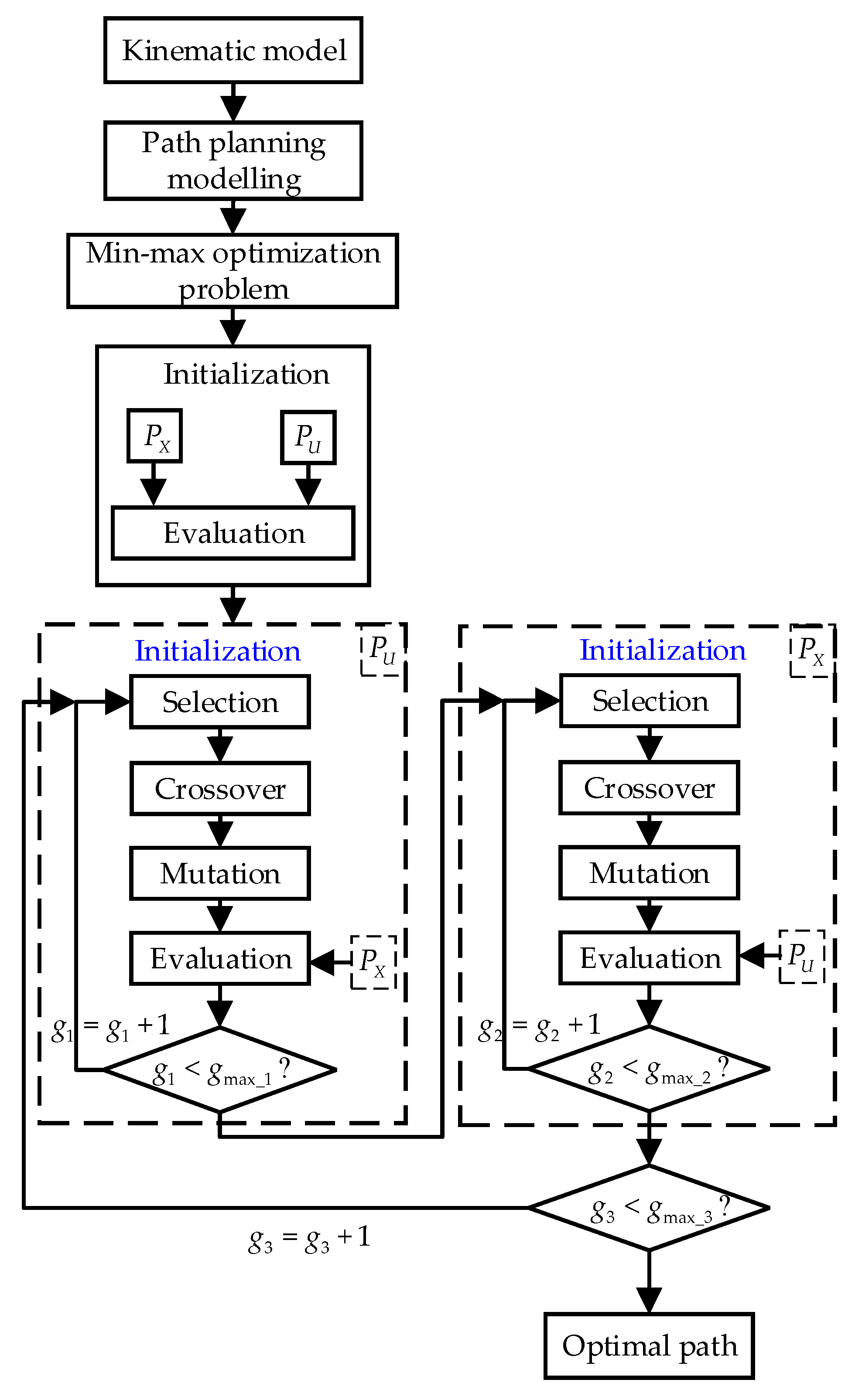
Figure 4 gives the robust optimization design flowchart of the path planning for bionic robotic fish, algorithm 1 gives the corresponding steps in detail.

Algorithm 1: Robust optimization design for path planning

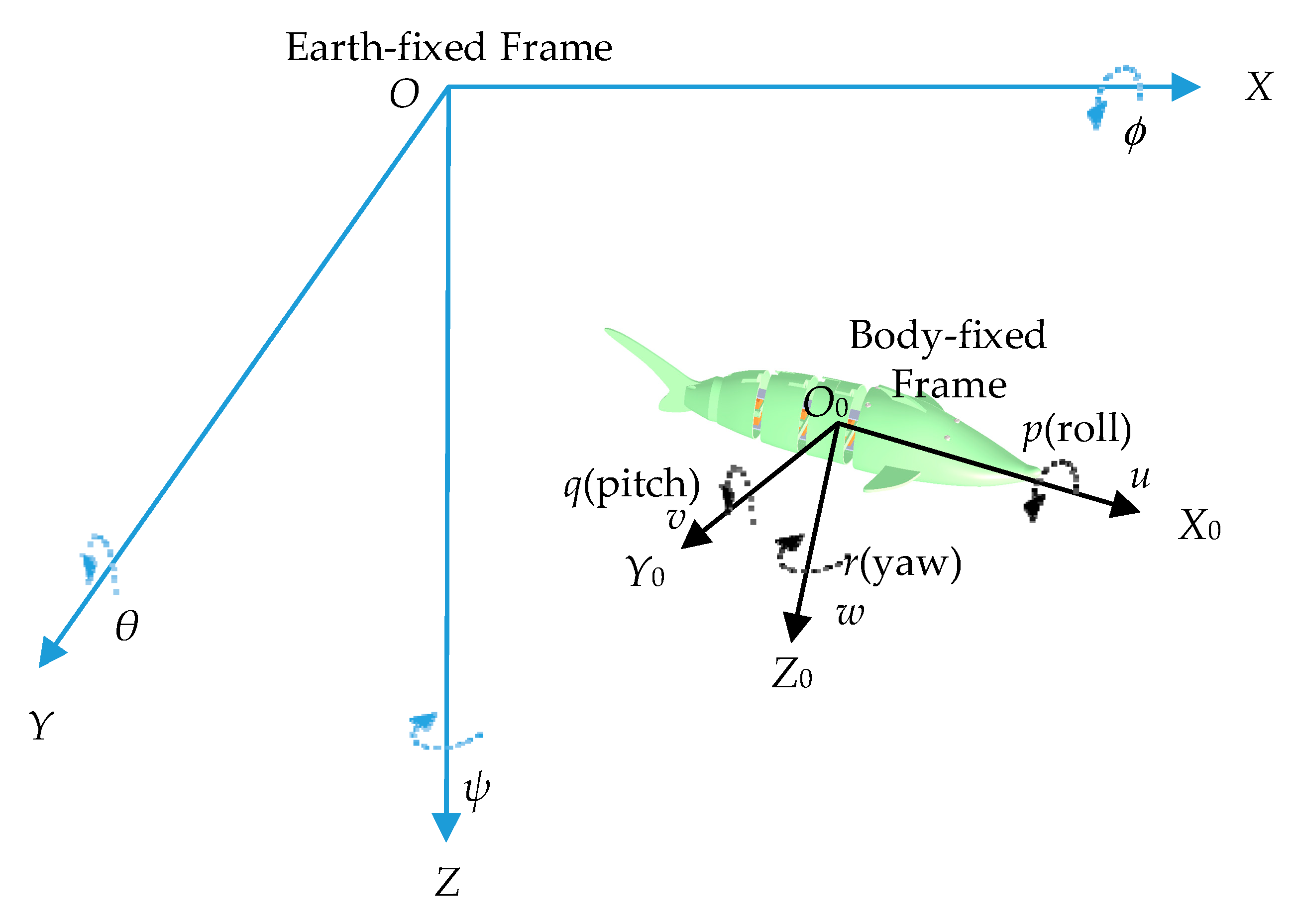
1: Modelling the environment for bionic robotic fish, establishing the two coordinate systems of the earth-fixed frame and the body-fixed frame; 2: Selecting the path energy consumption as the objective function of the path planning for bionic robotic fish; 3: Based on the established Kinematic model for bionic robotic fish, establishing path planning model (9) in the light of three basic elements of objective function, decision variables and constrains; 4: Considering the uncertainty of ocean currents, obtaining the robust optimization problem (19) for path planning of bionic robotic fish; 5: Initializing the parameters such as population size, the maximum number of iterations and so on; 6: Creating two populations $P_U$ and $P_X$, obtaining multiple collision-free initial paths based on the fitness functions (20) and (21); 7: Evaluating $P_U$ after selection, crossover and mutation operations based on (21); 8: If $g_1$ is smaller than $g_{\max \_1}$, setting $g_1=g_1+1$, go to step 7; otherwise go to next step; 9: Evaluating $P_X$ after selection, crossover and mutation operations based on (20); 10: If $g_2$ is smaller than $g_{\max \_2}$, setting $g_2=g_2+1$, go to step 9; otherwise go to next step; 11: If $g_3$ is smaller than $g_{\max \_3}$, setting $g_3=g_3+1$, go to step 7; otherwise go to next step; 12: Obtaining the optimal path.

5. Simulation Results and Analysis

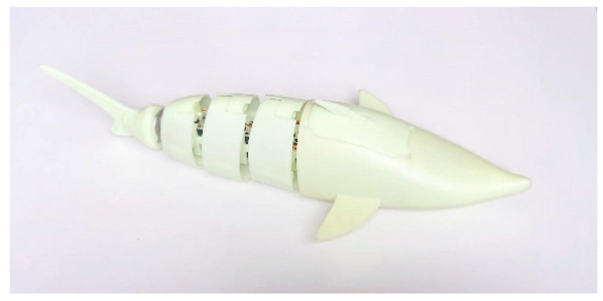
In this section, different scenarios are given to illustrate the performance of the proposed robust optimization design for the path planning of bionic robotic fish. Figure 5 shows the designed bionic robotic fish, the total length, width, and height are 0.617 $\mathrm{m}$, 0.239 $\mathrm{m}$, and 0.155 $\mathrm{m}$ respectively. It assumes that the population size is 100 and the maximum number of iterations is 200 for the co-evolutionary genetic algorithm.

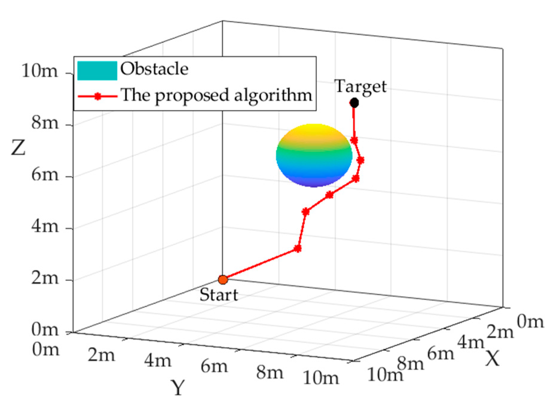
To test the performance of the proposed algorithm for path planning of bionic robotic fish in the environment with obstacle and ocean currents, it assumes that the ocean current is in the range of $[0, 0.1]$ $\mathrm{m}/\mathrm{s}$, whose direction is stochastic. Figure 6 shows that the bionic robotic fish works in the three-dimensional environment with $10 \mathrm{m}\times 10 \mathrm{m}\times 10 \mathrm{m}$. The center position is $(7 \mathrm{m}, 7 \mathrm{m}, 7 \mathrm{m})$ and radius is 1.2 $\mathrm{m}$ for the spherical obstacle. The start and target points are $(0 \mathrm{m}, 0 \mathrm{m}, 0 \mathrm{m})$ and $(10 \mathrm{m}, 10 \mathrm{m}, 10 \mathrm{m})$ respectively, the velocity is 0.2 $\mathrm{m}/\mathrm{s}$ for the bionic robotic fish. Figure 6 gives the obtained optimal path by the proposed algorithm, the corresponding path length is 17.89 m. It can be seen that the bionic robotic fish can obtain a non-collision path with the performance of short path length in the environment with the worst ocean currents. If the components of ocean currents $u_c$, $v_c$ and $w_c$ are 0.05 $\mathrm{m}/\mathrm{s}$, 0.06 $\mathrm{m}/\mathrm{s}$, 0 $\mathrm{m}/\mathrm{s}$ in practice, respectively. The energy consumption is 1.0619 $\mathrm{J}$ for the obtained optimal path by the proposed algorithm. The results show that the proposed algorithm can obtain a safety and smoothness path with low energy consumption in the presence of ocean currents.

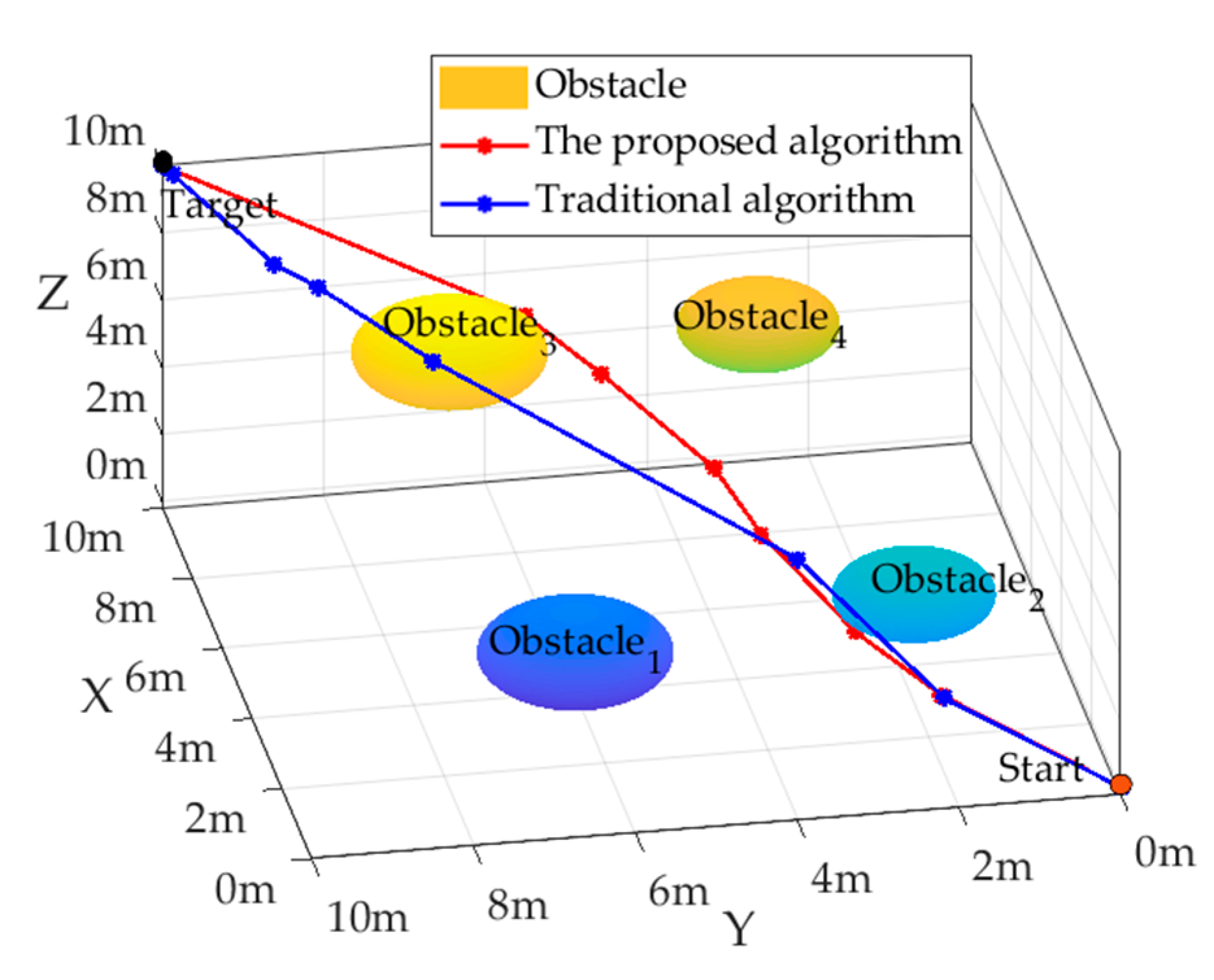
In order to further test the performance of the proposed algorithm, it assumes that there are four obstacles in the environment, the ocean currents are in the range of $[0, 0.1]$ $\mathrm{m}/\mathrm{s}$, whose direction is stochastic. The bionic robotic fish works in the three-dimensional environment with $10 \mathrm{m}\times 10 \mathrm{m}\times 10 \mathrm{m}$, the basic parameters of the obstacles are given in

Table 1. Basic parameters of the obstacles in Figure 7.

Serial Number	Coordinate Position of the Obstacle Center ($\mathbf{m}$)	Radius ($\mathbf{m}$)
Obstacle1	(4 m, 6 m, 1 m)	1.2 m
Obstacle2	(3 m, 2 m, 3 m)	1 m
Obstacle3	(7 m, 7 m, 7 m)	1.2 m
Obstacle4	(8 m, 3 m, 6 m)	1 m

. The start and target points are $(0 \mathrm{m}, 0 \mathrm{m}, 0 \mathrm{m})$ and $(10 \mathrm{m}, 10 \mathrm{m}, 10 \mathrm{m})$ respectively, the velocity of the bionic robotic fish is 0.2 $\mathrm{m}/\mathrm{s}$. Figure 7 gives the obtain optimal path by the proposed algorithm, the corresponding path length is 17.98 $\mathrm{m}$. It can be seen that the proposed algorithm can obtain the safe path under the condition of multiple obstacles and ocean currents. Figure 8 also gives the optimal path by the traditional PSO algorithm without considering the ocean currents (the blue curve), the corresponding path length is 17.73 m. If the components of ocean currents $u_c$, $v_c$ and $w_c$ are 0.071 $\mathrm{m}/\mathrm{s}$, 0.036 $\mathrm{m}/\mathrm{s}$, 0 $\mathrm{m}/\mathrm{s}$ in practice respectively. The energy consumption is 1.079 $\mathrm{J}$ for following the obtained optimal path by the proposed algorithm, the energy consumption is 1.083 $\mathrm{J}$ for following the obtained optimal path by the traditional algorithm. It can be seen that the energy consumption is smaller by the proposed algorithm than the traditional method. The main reasons are given as follows: for the proposed algorithm in this paper, it obtains the best solution in the worst case by the proposed algorithm, if the ocean currents are in the range of the given cases, the path planning design can satisfy the requirements for reducing energy consumption. The results show that the proposed algorithm is robust enough to be used in complex environments and can saving energy when lacking real time data about the environment with ocean currents.

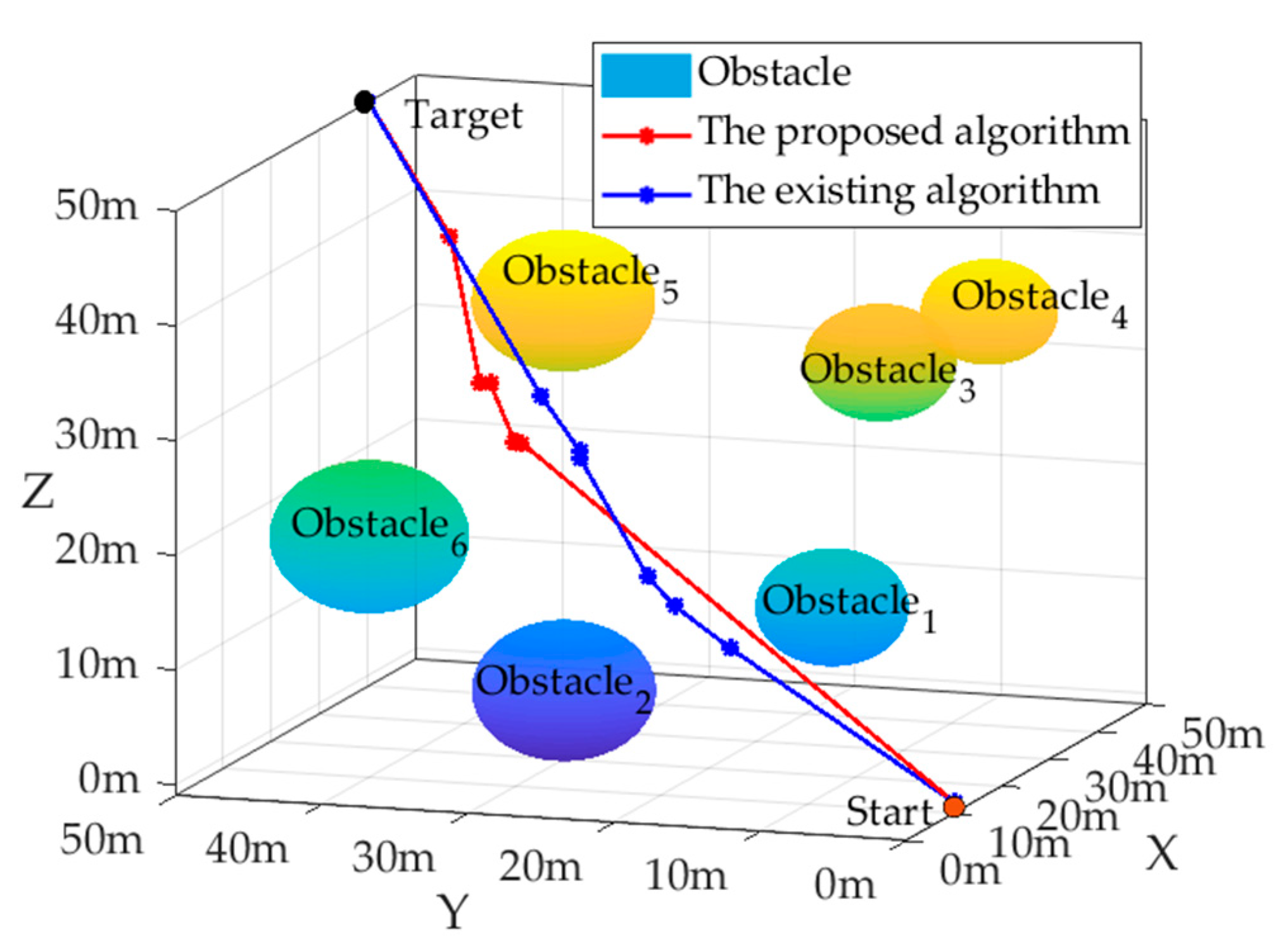
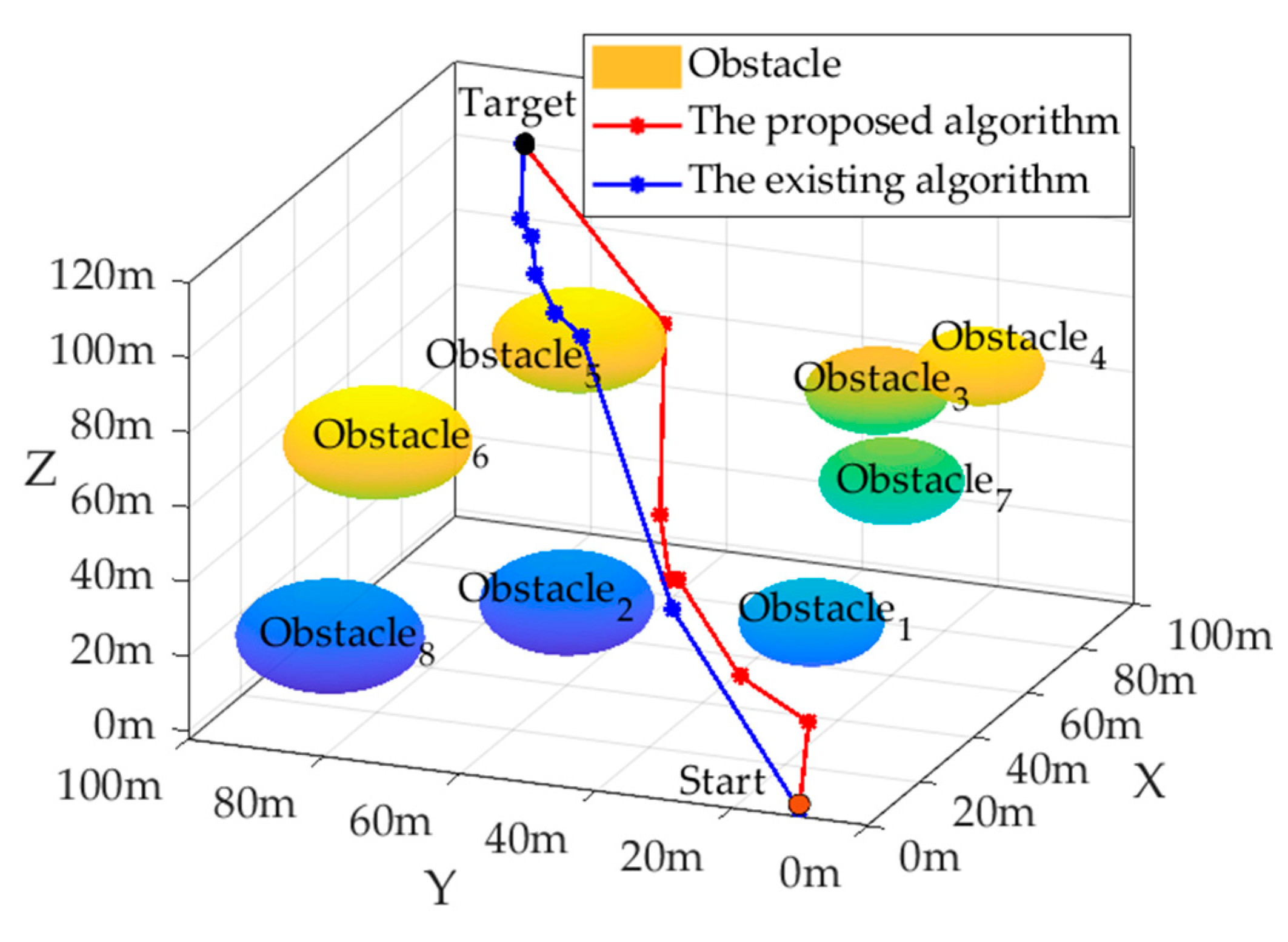
In order to further verify the proposed algorithm in the environment with ocean currents, some comparisons are given for the proposed algorithm and the existing algorithms. It assumes that the bionic robotic fish works in the three-dimensional environment with $50 \mathrm{m}\times 50 \mathrm{m}\times 50 \mathrm{m}$, the start and target points are $(10 \mathrm{m}, 0 \mathrm{m}, 0 \mathrm{m})$ and $(40 \mathrm{m}, 50 \mathrm{m}, 50 \mathrm{m})$ respectively, the velocity of the bionic robotic fish is 0.2 $\mathrm{m}/\mathrm{s}$. The ocean currents are in the range of $[0, 0.1]$ $\mathrm{m}/\mathrm{s}$, whose direction is stochastic.

Table 2. The basic parameters of the obstacles in Figure 8.

Serial Number	Obstacle Center ($\mathbf{m}$)	Obstacle Radius ($\mathbf{m}$)
Obstacle1	(15 m, 10 m, 15 m)	5 m
Obstacle2	(20 m, 30 m, 5 m)	6 m
Obstacle3	(40 m, 15 m, 30 m)	5 m
Obstacle4	(40 m, 7.5 m, 35 m)	4.5 m
Obstacle5	(35 m, 35 m, 35 m)	6 m
Obstacle6	(10 m, 40 m, 20 m)	6.5 m

gives the basic parameters of the obstacles of the path planning for bionic robotic fish. In practice, if the components of ocean currents $u_c$ is 0.03 $\mathrm{m}/\mathrm{s}$, $v_c$ is 0.07 $\mathrm{m}/\mathrm{s}$ and $w_c$ is 0 $\mathrm{m}/\mathrm{s}$. Figure 8 shows the comparison results between the proposed and existing IQPSO algorithms [8]. It can be seen that it can obtain a non-collision path by the proposed algorithm, the corresponding path energy consumption is 4.68 $\mathrm{J}$, path length is 80.88 $\mathrm{m}$. By using the existing IQPSO algorithm, the corresponding path energy consumption is 4.85 $\mathrm{J}$, path length is 79.3 $\mathrm{m}$. Compared with the results of the existing IQPSO algorithm, although the length of the planed path is larger by the proposed algorithm, the energy consumption is smaller. This means that the obtained optimal path by the existing algorithm may consume more consumption without considering the effects of ocean currents.

It assumes that the bionic robotic fish works in the three-dimensional environment with $100 \mathrm{m}\times 100 \mathrm{m}\times 120 \mathrm{m}$, the ocean currents are in the range of $[0, 0.1]$ $\mathrm{m}/\mathrm{s}$, whose direction is stochastic. The start and target points are $(10 \mathrm{m}, 0 \mathrm{m},0 \mathrm{m})$ and $(100 \mathrm{m}, 90 \mathrm{m}, 100 \mathrm{m})$ respectively.

Table 3. The basic parameters of the obstacles in Figure 9.

Serial Number	Obstacle Center ($\mathbf{m}$)	Obstacle Radius ($\mathbf{m}$)
Obstacle1	(30 m, 20 m, 30 m)	10 m
Obstacle2	(40 m, 60 m, 20 m)	12 m
Obstacle3	(80 m, 30 m, 60 m)	10 m
Obstacle4	(80 m, 15 m, 70 m)	9 m
Obstacle5	(70 m, 70 m, 70 m)	12 m
Obstacle6	(20 m, 80 m, 70 m)	13 m
Obstacle7	(60 m, 20 m, 50 m)	10 m
Obstacle8	(15 m, 85 m, 20 m)	13 m

gives the obstacles parameters for path planning for bionic robotic fish. For the existing QPSO algorithm [18] to design the path planning with fixed value of ocean currents. It sets the ocean current is 0.1 $\mathrm{m}/\mathrm{s}$, the angle is ${180}^{\circ }$ between the ocean current direction and the Y-axis; the angle is ${90}^{\circ }$ between the ocean current direction and X-axis; the angle is ${90}^{\circ }$ between the ocean current direction and the Z-axis. In practice, if the components of ocean currents $u_c$ is 0.066 $\mathrm{m}/\mathrm{s}$, $v_c$ is 0.045 $\mathrm{m}/\mathrm{s}$ and $w_c$ is 0 $\mathrm{m}/\mathrm{s}$. Figure 9 gives the optimal paths by the proposed and the existing QPSO algorithms [18] for the bionic robotic fish. By using the proposed algorithm, the corresponding energy consumption is 9.822 $\mathrm{J}$. The energy consumption is 9.994 $\mathrm{J}$ by using the existing QPSO algorithm. Compared with the optimal results by the existing algorithm, the energy consumption is smaller by the proposed algorithm. It has good optimization performance of energy consumption by the proposed algorithm for the path planning. The main reason is given as follows, the existing algorithm designs the path planning based on the fixed ocean currents, however, it doesn’t consider the influence with the variable ocean currents in practice, which decrease the optimization performance of the obtained optimal path.

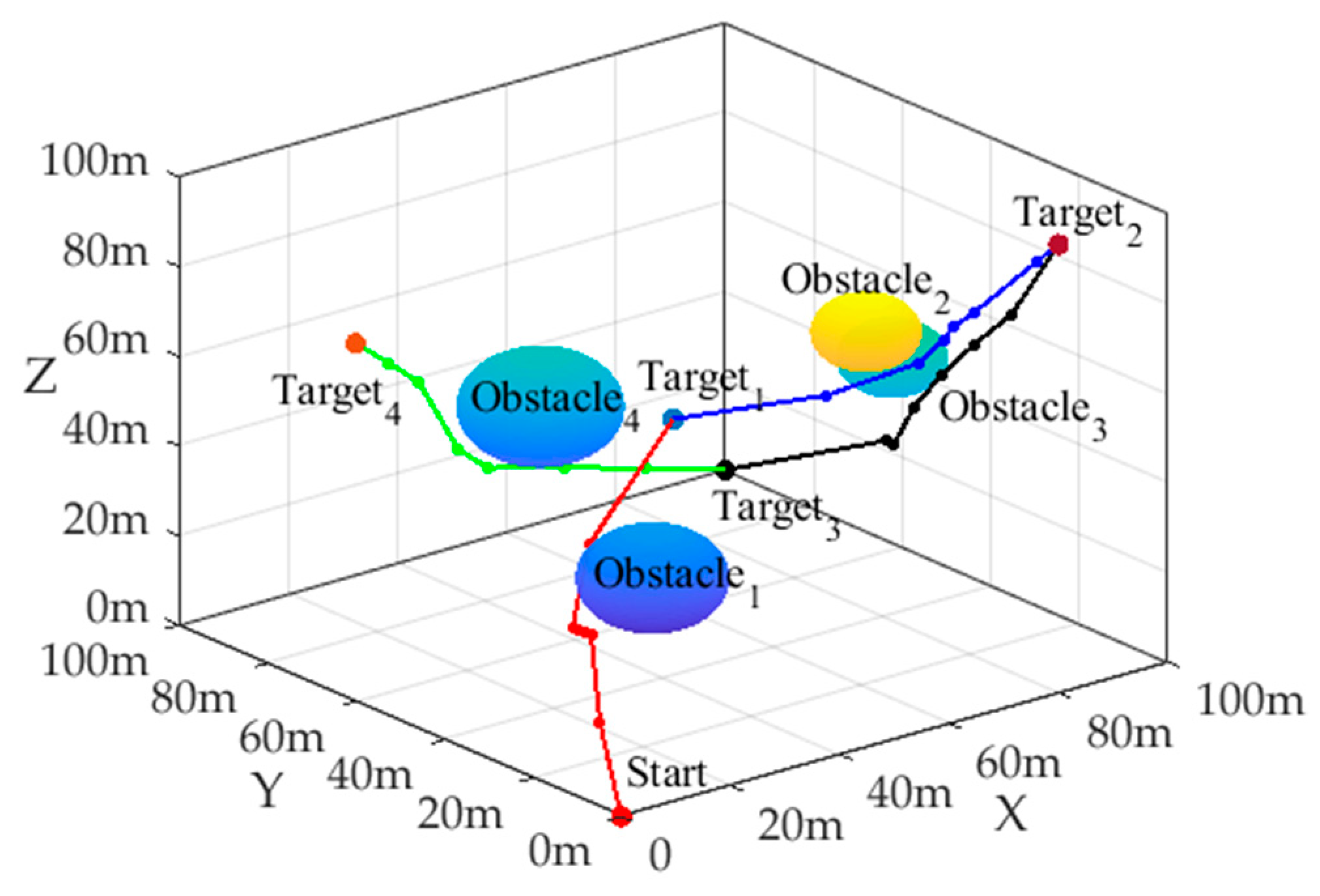
In practice, the bionic robotic fish may need to move from the start point to different targets for detection in sequence. It assumes that the bionic robotic fish works in the three-dimensional environment with $100 \mathrm{m}\times 100 \mathrm{m}\times 100 \mathrm{m}$ and that the ocean currents are in the range of $[0, 0.1]$ $\mathrm{m}/\mathrm{s}$, whose direction is stochastic. There are multiple targets and obstacles, the bionic robotic fish must get through these target points according to the order ${\mathrm{Target}}_1\to {\mathrm{Target}}_2\to \cdots \to {\mathrm{Target}}_4$. The start point is $(0 \mathrm{m}, 0 \mathrm{m}, 0 \mathrm{m})$ and the target points are $(50 \mathrm{m}, 50 \mathrm{m}, 50 \mathrm{m})$, $(80 \mathrm{m}, 0 \mathrm{m}, 100 \mathrm{m})$, $(100 \mathrm{m}, 100 \mathrm{m}, 0 \mathrm{m})$, $(0 \mathrm{m}, 60 \mathrm{m}, 80 \mathrm{m})$ for target₁ to target₄ respectively. The parameters for the obstacles are given in

Table 4. The basic parameters of the obstacles in Figure 10.

Serial Number	Obstacle Center ($\mathbf{m}$)	Obstacle Radius ($\mathbf{m}$)
Obstacle1	(30 m, 30 m, 30 m)	11 m
Obstacle2	(65 m, 25 m, 75 m)	8 m
Obstacle3	(90 m, 50 m, 50 m)	8 m
Obstacle4	(50 m, 80 m, 40 m)	12 m

. The velocity for bionic robotic fish is 0.2 $\mathrm{m}/\mathrm{s}$. Figure 10 gives the path planning for the bionic robotic fish to arrive at different targets in sequence, the optimal path energy consumption is 22.75 $\mathrm{J}$ and path length is 457.09 $\mathrm{m}$ by the proposed algorithm. One can see that the proposed algorithm can deal with the path planning problem for bionic robotic fish through the targets in sequence in the environment with ocean currents effectively.

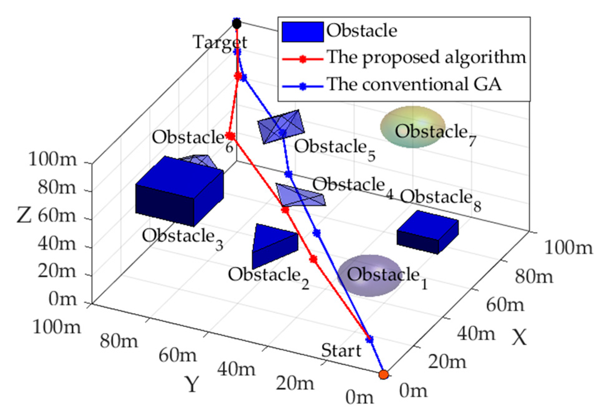
It assumes that the bionic robotic fish works in the three-dimensional environment with $100 \mathrm{m}\times 100 \mathrm{m}\times 100 \mathrm{m}$ and that the ocean currents are in the range of $[0, 0.1]$ $\mathrm{m}/\mathrm{s}$, whose direction is stochastic. The start and target points are $(0 \mathrm{m}, 0 \mathrm{m},0 \mathrm{m})$ and $(100 \mathrm{m}, 100 \mathrm{m}, 100 \mathrm{m})$. In practice, if the components of ocean currents $u_c$ is 0.06 $\mathrm{m}/\mathrm{s}$, $v_c$ is 0.04 $\mathrm{m}/\mathrm{s}$ and $w_c$ is 0 $\mathrm{m}/\mathrm{s}$. Figure 11 shows the comparison results between the proposed and conventional genetic algorithms, it can be seen that it can obtain a non-collision path by the proposed algorithm, the corresponding path energy consumption is 10.81 $\mathrm{J}$, path length is 179.86 $\mathrm{m}$. By using the conventional genetic algorithm, the corresponding path energy consumption is 10.99 $\mathrm{J}$, path length is 179.02 $\mathrm{m}$. Compared with the conventional genetic algorithm, it can be seen that the path length and energy consumption are smaller by the proposed algorithm. The main reason is given as follows, the conventional genetic algorithm designs the path planning without considering the effect of ocean currents, which decreases the optimization performance of the obtained optimal path. Ocean currents affect the energy consumption of the path planning in practice.

Table 5. Energy consumptions with different ocean currents.

	Considerations	$\left|{\mathit{V}}_c\right|=[0,0.2]$$\mathbf{m}/\mathbf{s}$, ${\mathit{v}}_{\mathit{f}}=0.3$$\mathbf{m}/\mathbf{s}$
Actual Situations
Ocean current ($\mathrm{m}/\mathrm{s}$)		[0.05, 0.05, 0]	[0.1, 0.1, 0]	[0.12, 0.13, 0.09]	[0.08, 0.16, 0.08]	[0.18, 0.05, 0.09]
Energy consumption ($\mathrm{J}$)		20.96	28.53	33.81	34.22	36.76

gives the energy consumption with different ocean currents. It assumes that the design conditions are given as follows: the magnitude of ocean current velocity $\left|V_c\right|=[0, 0.2]$ $\mathrm{m}/\mathrm{s}$, the velocity is $v_f=0.3$ $\mathrm{m}/\mathrm{s}$ for the bionic robotic fish. The optimal path length is 188.72 $\mathrm{m}$ by the proposed algorithm. In practice, with the increasing of the values of ocean currents, the energy consumption increases. For example, if the components of ocean currents $u_c$ is 0.05 $\mathrm{m}/\mathrm{s}$, $v_c$ is 0.05 $\mathrm{m}/\mathrm{s}$ and $w_c$ is 0 $\mathrm{m}/\mathrm{s}$; the path energy consumption is 20.96 $\mathrm{J}$. If the components of ocean currents $u_c$ is 0.1 $\mathrm{m}/\mathrm{s}$, $v_c$ is 0.1 $\mathrm{m}/\mathrm{s}$ and $w_c$ is 0 $\mathrm{m}/\mathrm{s}$; the path energy consumption is 28.53 $\mathrm{J}$, which is larger.

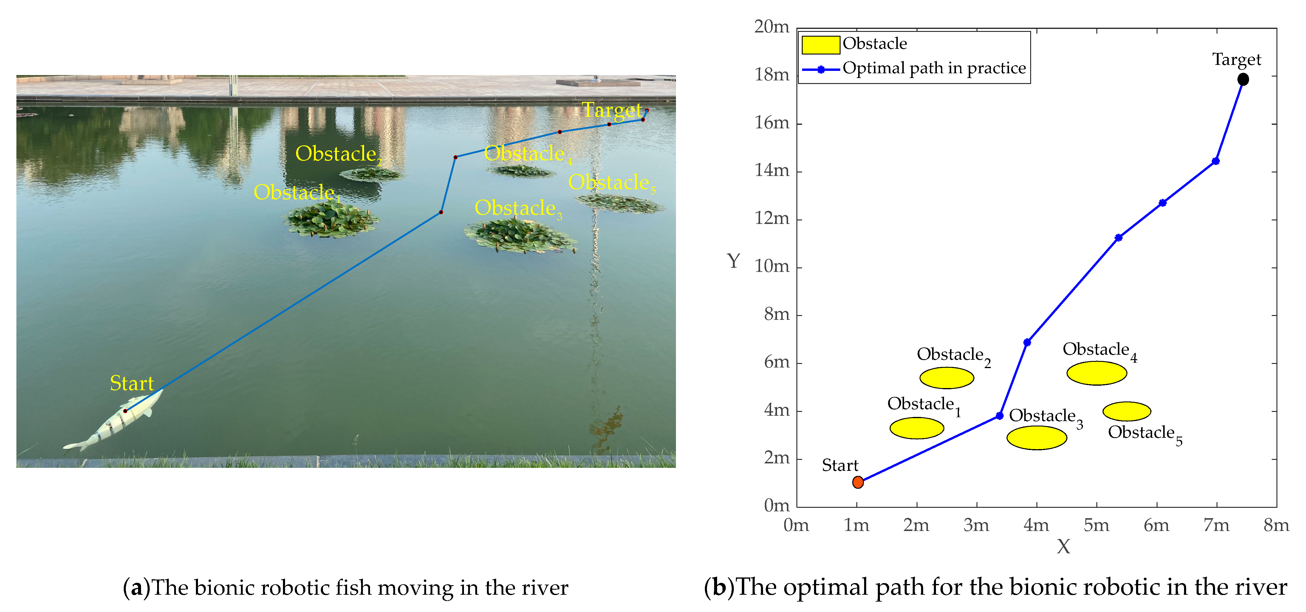
In order to test the effectiveness of the proposed algorithm in practice, the proposed algorithm is used for our designed bionic robotic fish in the river of our university. Based on the distance measuring equipment, Figure 12 gives the map for the path planning of the bionic robotic fish. Figure 12 shows the real bionic robotic fish moving in the river,

Table 6. The basic parameters of the obstacles in Figure 12.

Serial Number	Obstacle Center ($\mathbf{m}$)	Radius ($\mathbf{m}$)
Obstacle1	(2 m, 3.3 m, 0 m)	0.45 m
Obstacle2	(2.5 m, 5.4 m, 0 m)	0.45 m
Obstacle3	(4 m, 2.9 m, 0 m)	0.5 m
Obstacle4	(5 m, 5.5 m, 0 m)	0.5 m
Obstacle5	(5.5 m, 4 m, 0 m)	0.4 m

shows the basic parameters of the obstacles, the start and goal points are $(1 \mathrm{m}, 1 \mathrm{m}, 0 \mathrm{m})$ and $(7 \mathrm{m}, 17 \mathrm{m}, 0 \mathrm{m})$ respectively. It assumes that the design consideration of ocean currents is in the range of $[0, 0.05]$ $\mathrm{m}/\mathrm{s}$, the direction of ocean currents is stochastic. In order to better illustrate the effectiveness of the proposed algorithm, it sets that the designed bionic robotic fish works in a plane without up and down motion. In Figure 12, based on the optimal path planning with the worst ocean currents, it obtains a non-collision path in practice, the corresponding path length is 17.27 $\mathrm{m}$, the energy consumption is 0.83 $\mathrm{J}$. In practice, the energy is 0.69 without the ocean currents. Without the real time value of ocean currents, the bionic robotic fish can obtain a non-collision path with low energy consumption.

6. Conclusions

Path planning is the premise for bionic robotic fish to accomplish missions in the three-dimensional environment. In the complex underwater environment, the uncertain ocean currents are inevitable in practice, whose influence cannot be ignored on path planning for bionic robotic fish. In this paper, in order to solve the path planning problem for bionic robotic fish with ocean currents, it selects energy consumption as the object function; smoothness and safety factor are selected as constraint conditions. A general path planning problem is formed in the light of the three basic elements of decision variables, objective functions, and constraint conditions. Considering the uncertainty of ocean currents, it presents a robust optimization problem, which is solved by the proposed co-evolutionary genetic algorithm, an optimal path can be obtained by finding the best solution in the worst cases. Different scenarios illustrate that it can obtain the optimal path with strong robustness by the proposed robust optimization design algorithm for the path planning for bionic robotic fish in the environment with ocean currents. Compared with the results by existing methods, it obtains optimal paths with better optimization performance by the proposed algorithm. In this paper, the proposed algorithm cannot deal with the path planning with moving obstacles effectively. Therefore, we will propose a dynamic programming algorithm to solve this problem in the future work. We will also plan to use the back propagation neural network to establish the energy consumption model. Because the input and output data are obtained from the engineering practice, the established model is more realistic.