A Review of Recent Machine Learning Advances for Forecasting Harmful Algal Blooms and Shellfish Contamination

Abstract

Harmful algal blooms (HABs) are among the most severe ecological marine problems worldwide. Under favorable climate and oceanographic conditions, toxin-producing microalgae species may proliferate, reach increasingly high cell concentrations in seawater, accumulate in shellfish, and threaten the health of seafood consumers. There is an urgent need for the development of effective tools to help shellfish farmers to cope and anticipate HAB events and shellfish contamination, which frequently leads to significant negative economic impacts. Statistical and machine learning forecasting tools have been developed in an attempt to better inform the shellfish industry to limit damages, improve mitigation measures and reduce production losses. This study presents a synoptic review covering the trends in machine learning methods for predicting HABs and shellfish biotoxin contamination, with a particular focus on autoregressive models, support vector machines, random forest, probabilistic graphical models, and artificial neural networks (ANN). Most efforts have been attempted to forecast HABs based on models of increased complexity over the years, coupled with increased multi-source data availability, with ANN architectures in the forefront to model these events. The purpose of this review is to help defining machine learning-based strategies to support shellfish industry to manage their harvesting/production, and decision making by governmental agencies with environmental responsibilities.

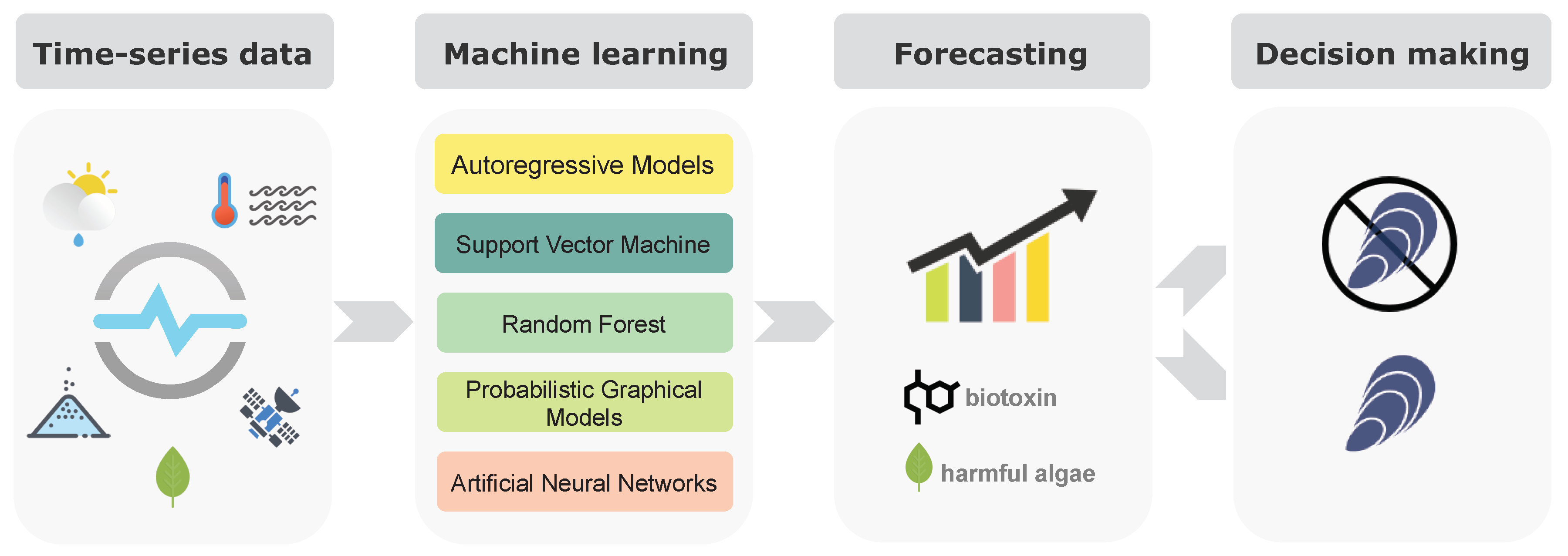
1. Impact of Harmful Algal Blooms (HABs) on Shellfish Safety

Shellfish farming and shellfish harvesting from natural seed banks have been growing in recent years as a response to the increasing worldwide demand for seafood products [1]. According to estimations of the United Nations, the world human population will reach 9.7 billion people in 2050 [2], which represents a significant challenge to guarantee food security and safety. While wild-capture has limited chances of growing and developing new sustainable fisheries, shellfish farming is able to respond to new challenges in terms of both economic and environmental aspects. Shellfish farming shows multiple benefits, such as no need for freshwater input, and limited artificial feed. Shellfish are filter-feeding organisms, relying on the plankton available in the water column to grow [3]. However, among a plethora of phytoplankton species occurring in seawater, a few may produce toxic compounds and contaminate shellfish. Harmful algal blooms (HABs) are a natural phenomenon occurring in all aquatic environments (fresh, brackish, and marine waters) characterized by relatively fast proliferation of toxic phytoplankton. The frequency and intensity of HAB events are increasing in response to global warming and other climate change conditions, with consequences to environment and shellfish safety. During these events, shellfish may accumulate high concentrations of natural toxins and remain contaminated and unsafe for human consumption, jeopardizing shellfish farming [4].

Consumption of contaminated shellfish can cause serious health problems. The most common poisonings are known by their symptoms, namely diarrhetic shellfish poisoning (DSP), amnesic shellfish poisoning (ASP), and paralytic shellfish poisoning (PSP) [4]. To safeguard public health and minimize the risk of acute intoxication, shellfish are routinely monitored for HAB-derived marine biotoxins in most coastal countries. In order to ensure that safe concentrations are not exceeded and contaminated shellfish do not enter the markets, a series of directives establishing sampling frequency, analytical methods of reference for toxins determination, and safety limits are defined in the EU Regulations [5,6].

The current strategy has been highly effective in terms of consumer protection. The number of reported cases of shellfish food poisonings during the last decade is low, and in most occasions, intoxication results from not respecting or misunderstanding of harvesting closures [7,8]. However, the system is based on a reactive approach, responding only after shellfish contamination is verified. Sudden and prolonged closures to shellfish harvesting due to temporary contamination with marine toxins leads to severe economic losses and disruptions to coastal towns’ social fabric and cultural identity. Therefore, it becomes necessary to develop proactive strategies to predict the environmental changes, HAB formation, and shellfish contamination to anticipate and mitigate these negative impacts. The possibility of knowing in advance when harvesting will be prohibited, and for how long, will benefit the productive and recreational sectors. Entities with activities related to shellfish farming will be able to take proper actions in terms of production management, stock distribution or storage, reducing production waste and economic losses.

2. Forecasting HABs and Shellfish Biotoxin Contamination

Official control data and environmental parameters are collected at regular time intervals, making time-series modeling a natural first statistical learning choice. Time series analysis and forecasting aims at understanding the past and predicting the future based on past observations, enabling managers and policymakers to make decisions with sound scientific support. In the particular context of HAB and shellfish contamination forecasting, the goal is to make use of available time-series data via statistical and machine learning methods to make predictions on future events and guide decision on harvesting permissions (Figure 1).

Shellfish contamination often exhibits a cyclic or seasonal pattern due to its relation to climate and biological variables [9]. Since HABs are the source of the biotoxins responsible for shellfish contamination, great efforts have been put to develop early warning systems for HABs (e.g., [10,11]). It is reasonable that first attempts have been focused on HAB modeling, their prediction, persistence, and spread. However, HAB prediction may fail to estimate shellfish contamination, as HAB species greatly vary on toxin production, and shellfish accumulation/elimination dynamics vary among species. The role of other drivers, including climate and environmental variables, has been investigated as predictors of biotoxin contamination by multivariate time-series modeling based on a range of variables measured over time (e.g., [12,13,14]). The following review covers past and current directions in time-series forecasting of algal bloom events and shellfish contamination by marine biotoxin. Our focus is on machine learning (ML) methods because these are generic methods that can be applied to this whole class of problems. Furthermore, these models have the ability to handle big data and are flexible in selecting/excluding features.

ML models have some advantages in comparison to other approaches that have been used to model algal dynamics. One example are process-based models—mathematical models based on prior assumptions about the interactions and mechanisms that regulate the phytoplankton compartment. Since these mechanisms are complex and non-linear, these models have difficulties in accurately reproducing phytoplankton dynamics [15]. ML methods, on the other hand, are known to be effective in handling complex, non-linear and noisy datasets, especially when underlying physical relationships are not fully understood [16]. Moreover, they do not require the a priori assumptions used by the process-based models [12]. Additionally, ML models can be applied to virtually any data, eliminating the need to specify assumptions regarding the underlying statistical distribution of the data, as in traditional statistical models [17]. Despite the many advantages of ML methods, there has been a large amount of work to establish HAB dynamics using process-based and traditional statistical models. For a review on the use of these methods for HAB modeling see Franks (2018) [18].

3. Time-Series Forecasting Methods

In a time series forecasting problem, given an observed time series $\{x_1,x_2,\dots ,x_T\}$, one wishes to forecast one or more future values, $\{x_{T+h},x_{T+h+1},\dots \}$, where the integer h is called the lead time or the forecasting horizon [19]. Forecasting methods may be classified into univariate methods and multivariate methods. In univariate methods, forecasts depend only on the present and past values of the single series being forecasted. In multivariate methods, forecasts of a given variable depend, at least partly, on values of one or more additional time-series variables, called predictor or explanatory variables [19].

Multivariate time series (MTS) occur when multiple variables are observed over time. MTS data are common in various fields, such as the traffic flows on highways, stock market prices, and the temperatures across different cities. In such applications, users are usually interested in the forecasting of new trends based on historical observations. One major research challenge often faced in MTS forecasting problems is how to capture and leverage the complex interdependencies between different variables. The better the interdependencies among different series are modeled, the more accurate the forecasting can be, and so many models that try to capture these relationships have been developed [20,21].

In order to assess the performance of the forecasting models, i.e., how accurate the models are when forecasting future values, it is common to use evaluation metrics. These metrics usually measure the forecast errors, which are the difference between the actual values and their forecasts [22]. Several error measures can be used to assess forecasting performance, depending on the objective of the forecast. In a regression problem, in which the values to be predicted are continuous, the root mean square error (RMSE) and the mean absolute error (MAE) are two examples [22]. In a classification problem, in which the values to be predicted belong to discrete categories, an example of a metric used to assess the forecasting performance is the classification accuracy, which measures the percentage of correctly classified values.

3.1. Autoregressive Models

A traditional approach to model univariate time series is to use an autoregressive model—a linear model in which the present value of a variable is explained by its own past values [23]. In an autoregressive model of order p, AR(p), the value of $X_t$ is obtained through a weighted linear sum of the past p values plus white noise,

$$X_t={\varphi }_1{X}_{t-1}+{\varphi }_2{X}_{t-2}+\dots +{\varphi }_p{X}_{t-p}+{\epsilon }_t=\sum _{i=1}^p\left({\varphi }_i{X}_{t-i}\right)+{\epsilon }_t,$$

(1)

where ${\epsilon }_t$, called a random shock, denotes a purely random process, i.e., a process defined as a sequence of uncorrelated, identically distributed random variables with zero mean and constant variance [19].

A more general class of autoregressive models for time series analysis is the autoregressive integrated moving average (ARIMA) model [24]. ARIMA directly models the autocorrelation of the series values, as well as the autocorrelations of the random shocks, ${\epsilon }_t$ [25]. An AR(p) model captures the autocorrelations of the series values up to lag p. Adding the autocorrelation terms for the random shocks up to lag q—called a moving average model, MA(q)—we obtain an autoregressive moving average (ARMA) model, ARMA($p,q$) [25],

$$X_t={\varphi }_1{X}_{t-1}+{\varphi }_2{X}_{t-2}+\dots +{\varphi }_p{X}_{t-p}+{\epsilon }_t+{\theta }_1{\epsilon }_{t-1}+{\theta }_2{\epsilon }_{t-2}+\dots +{\theta }_q{\epsilon }_{t-p}.$$

(2)

AR and ARMA models are only adequate for data without trend or seasonality. To circumvent this problem, an ARIMA model incorporates a preliminary step of differencing, which is performed before fitting the model. Differencing a time series consists of subtracting the prior observation to the current observation, that is, $\Delta x_t=x_t-x_{t-1}$. The order of differencing in an ARIMA($p,d,q$) model, d, indicates how many rounds of differencing are performed.

ARIMA is one of the most popular models for time series forecasting. Since it includes the AR (when $q=0$ and $d=0$), MA (when $p=0$ and $d=0$), and ARMA (when $d=0$) models, it is flexible and adaptable to various types of time series [26]. ARIMA attempts to filter out high-frequency noise in the data to detect local trends based on linear dependence in observations in the series. This model accommodates the dynamic behavior changing over time to predict future occurrences based on the recently changed relationships.

The problem of forecasting algal blooms has been approached via ARIMA models. Chen et al. (2015) [27] applied an ARIMA model to daily chlorophyll-a (chl-a) concentrations to obtain short-term predictions of algal blooms in Taihu Lake, China. The authors compared the proposed model to a multivariate linear regression (MVLR) model, which used several input variables, such as water temperature, water transparency, total inorganic nitrogen concentration, and phosphate concentration. The results showed that the ARIMA model outperformed the MVLR model with respect to multiple evaluation metrics.

ARIMA models can also be a source of data for more complex multivariate models, since many variables critical for HABs can be forecasted accurately using ARIMA on short time scales. One example of this approach is the work of Qin et al. (2017) [28], that proposed a hybrid model combining ARIMA with a deep belief network (DBN) [29], a type of deep neural network, for HAB prediction on two coastal areas in Zhejiang, China. In the proposed approach, the authors chose twelve environmental variables measured at one-week intervals and used the ARIMA model to forecast each variable up to ten weeks in advance. Then, the predicted values were used as input to a DBN. The DBN captured the complex non-linear relationships between the environmental factors and algal biomass, outputting the forecast for algal biomass up to ten-weeks ahead. The results showed that the proposed ARIMA-DBN model could reliably forecast the future trend of algal biomass, outperforming several other models, such as DBN, feed-forward neural network (FFNN; method described below), and ARIMA combined with an FFNN.

Despite its widespread application across many application domains, ARIMA is only able to model linear patterns in time series and cannot capture the non-linear patterns present in many complex systems (

Table 1. Strengths and weaknesses of time-series methods applied in studies to forecast HABs and shellfish contamination (ARIMA, Autoregressive Integrated Moving Average; VAR, Vector Autoregression; FFNN, Feed-Forward Neural Network; CNN, Convolutional Neural Network; RNN, Recurrent Neural Network; LSTM, Long Short-Term Memory).

Method	Strengths	Weaknesses	Ref.
Autoregressive Models
ARIMA	Needs a small amount of data, is simple, fast, flexible, and adaptable to various types of time series.	Cannot model non-linear patterns in time series and is not applicable to multivariate cases.	[27,28,30]
VAR	Applicable to multivariate time series, simple and flexible.	Is prone to overfit and cannot model non-linear patterns in time series.	[31]
Support Vector Machine	Models non-linear data, needs a small amount of data, generalizes well, and assures a global optimal solution.	Has a high computational cost and tends to overfit when applied to high-dimensional multivariate time series.	[32,33,34]
Random Forest	Models non-linear data, is robust and insensitive to missing data, and its outputs are easily interpretable.	Has a high computational cost and tends to overfit when applied to high-dimensional multivariate time series.	[12,13,35]
Probabilistic Graphical Models	Easy to incorporate diverse data types and to specify relations between variables. Explicitly probabilistic results.	Depends on a correct manual modeling of the relations between variables. A good estimate of the joint probability distributions may require a large data set, especially with complex models.	[36]
Artificial Neural Networks
FFNN	Models dynamic, non-linear and noisy data, has a low computational cost, is easy to set up, self-adaptable, self-organizing, and error tolerant.	Yields instable outputs, can produce a local minimum result, has a low efficiency and slow convergence speed, the parameter tuning is difficult.	[14,16,30,34,37,38,39,40,41,42,43,44]
CNN	Extracts important features from the data, can work with noisy data, has a small number of trainable weights and efficient training.	The receptive field size needs to be tuned carefully to use all relevant historical information, and struggles to capture long-term dependencies in the data.	[45]
RNN, LSTM	Captures temporal dependencies over variable periods of time.	Has a high complexity and computational cost.	[46,47,48,49]

). Moreover, ARIMA is not applicable to multivariate time series.

The vector autoregressive (VAR) model, which extends the AR model to the multivariate setting, emerged as a solution to address this latter issue. A VAR model is an n-variable, n-equation linear model in which each variable is explained by its own lagged values, plus current and past values of the remaining $n-1$ variables [23]. In a VAR model of order p, the the current values of a vector ${\mathbf{X}}_t=\left[X_{1,t},X_{2,t},\dots ,X_{n,t}\right]$ are given by

$${\mathbf{X}}_t={\varphi }_0+\sum _{i=1}^p\left({\varphi }_i{\mathbf{X}}_{t-i}\right)+{\mathbf{a}}_t,$$

(3)

where ${\varphi }_0$ is a n-dimensional constant vector, ${\varphi }_i$ are $n\times n$ matrices for $i>0$, and ${\mathbf{a}}_t$ are independent and identically distributed random vectors with mean zero and time invariant covariance matrix ${\Sigma }_a$ [50].

VAR is one of the most commonly used MTS models due to its simplicity and flexibility, and its properties have been broadly studied in the literature [24,51,52]. In the context of HAB forecasting, Lui et al. (2007) [31] developed a VAR model with exogenous variables (VARX) to predict algal blooms at Kat O, Hong Kong. The authors used daily and 2-h field monitoring data of water temperature, solar radiation, and wind speed as exogenous variables to predict one-step ahead chl-a fluorescence. The proposed approach had the advantage that the model parameters were interpretable, giving insights into the actual algal dynamics process. Even though the VARX model outperformed an artificial neural network approach proposed by Lee et al. (2004) [53] on the same data, it performed worse than a standard AR model.

VAR models have two main disadvantages (Table 1). First, the model capacity of VAR grows quadratically over the number of variables. Therefore, when applied to MTS with many variables, this model can have a large number of parameters, making it prone to overfitting [20,54], which means that the model adapts too much to the details in the data used for training, performing poorly on new data. Furthermore, VAR models are linear and thus fail to capture non-linear relationships among variables. The ability to capture non-linearity is especially important in the HAB and shellfish contamination forecasting problem, since the relationships between biological and environmental variables in ecosystems are often very complex and highly non-linear [55]. In order to handle the non-linear relationships involved in MTS, non-linear models have been proposed.

3.2. Support Vector Machine

A time series forecasting problem can be treated as a standard regression problem with time-varying parameters [20]. Thus, over the years, multiple non-linear regression methods have been proposed for time series forecasting tasks. One example is the support vector machine (SVM), introduced by Vapnik (1995) [56].

In a classification problem, the basic idea of SVM is to map the input data into a high-dimensional feature space, $\mathcal{F}$, using a fixed non-linear mapping, $\Phi$. In this high-dimensional space, the data can be separated using a linear hyperplane [57]. The projecting of the input data into the feature space can be done implicitly using a kernel function, which returns the inner product $\langle \Phi \left(x\right),\Phi \left(x^{\prime }\right)\rangle$ between the images of two data points, x and $x^{\prime }$, in the feature space. The learning process takes place in the feature space, and the data points only appear inside dot products with other points. This is computationally simpler than explicitly projecting x and $x^{\prime }$ into the feature space $\mathcal{F}$ [58]. In the case of a regression problem, SVM works similarly: the input data is mapped into a high-dimensional feature space via a non-linear mapping, and a linear regression is performed in this space [59].

SVM models have some advantages over artificial neural networks (ANNs; method described below) (Table 1), including good generalization ability, only requiring a small amount of training data and assurance of a global optimal solution [34]. Ribeiro and Torgo (2008) [32] compared the performance of three prediction models, SVM, ANN, and random forest (RF; method described below), on the task of predicting algal blooms. They used biweekly physical-chemical and microbiological variables collected in river Douro, Portugal, to predict the abundance values of seven micro-algae groups (Cyanobacteria, Cryptophyta, Euglenophyta, Chrysophyta, Dinophyta, Chlorophyta, and Diatom). The results showed that the proposed SVM model outperformed the other two approaches for almost all the micro-algae groups analyzed.

Vilas et al. (2014) [33] proposed a SVM model to predict Pseudo-nitzschia spp. blooms in the Galician coast, Spain. These blooms have adverse health and economic impacts, namely due to mussel contamination with ASP toxins. The authors used eight years of Pseudo-nitzschia abundance and associated meteorological and oceanographic data to predict Pseudo-nitzschia presence/below detection limit and bloom/no bloom situations. The bloom/no bloom models, that were trained using only the presence samples, showed a high predictive performance, which was superior to an ANN used in a previous study [60], and thus could offer useful information to the local shellfish industry. Li et al. (2014) [34] used monthly/biweekly water quality data to predict HABs in Tolo Harbour, Hong Kong, based on several machine learning methods, namely, SVM, FFNN, and a generalized regression neural network [61]. For both one- and two-weeks ahead predictions of chl-a, SVM showed the best performance among all the tested models, outperforming all the ANNs.

However, similar to VAR, the number of parameters in SVM models grows quadratically over the temporal window size and the number of variables, leading to high computational cost and risk of overfitting when dealing with high-dimensional MTS data [62] (Table 1). In fact, in the work of Li et al. (2014) [34], even though the SVR model outperformed the ANNs in all the used evaluation metrics, its running time was much higher.

3.3. Random Forest

Random forest (RF) is another non-linear regression model that can be used in time series forecasting problems. An RF is a machine learning model developed by Breiman (2001) [63], which easily adapts to non-linearities found in the data. The RF algorithm consists of ensembles of decision tree models. In a decision tree, the input data is recursively partitioned into two groups based on certain criteria until a predetermined stopping condition is met. A disadvantage of decision trees is that they are prone to overfitting, adapting too much to the details in the training data and performing poorly on new data. RF models address this issue by considering only a subset of the input data and building many individual trees [64]. In an RF model, each individual tree is built on a random sub-sampling of the input data. The final output of the model is then determined by aggregating the results generated by each tree making up the forest [35]. This method increases the robustness and generalization accuracy of individual decision trees [35,64] (Table 1).

Yajima and Derot (2018) [35] proposed an RF model to forecast algal blooms in the Urayama Reservoir (with fresh water) and the Lake Shinji (with saline water), Japan. The authors used monthly water records containing more than ten years of data to forecast chl-a concentration one to six months ahead. The results showed that the RF model could forecast the general trends of chl-a concentration. Moreover, the model allowed the authors to determine the most influential variables for the forecast: chemical and biochemical oxygen demand, pH, and total nitrogen/total phosphorus.

More recently, Derot et al. (2020) [12] proposed an RF model to forecast HABs caused by the toxic cyanobacterium Planktothrix rubescens in Lake Geneva. The goal was to lay the foundation for a HAB forecasting model to help local stakeholders managing the lake. The authors used 34 years of monthly/bi-monthly data of P. rubescens concentration, biological and physical-chemical variables. Using a K-means clustering algorithm [65], the P. rubescens concentration values were grouped into four categories, which were then used as the prediction target for an RF model. The results showed that the proposed approach could predict the concentration of harmful cyanobacteria over a year scale.

RF models have also been used for shellfish toxicity prediction. Harley et al. (2020) [13] used several environmental time series, such as sea surface temperature (SST), salinity, and air temperature, to predict the concentration of PSP toxins in blue mussels. The authors created an RF model to classify shellfish above and below a toxicity threshold one week in advance. However, a low classification accuracy was obtained (below 50%) for the out-of-sample hindcast.

3.4. Probabilistic Graphical Models

Alongside the remarkable development of machine learning algorithms to model time-series data, there is a growing need to understand the causal temporal relationships in complex systems. Temporal probabilistic graphical models have been proposed to infer the direction of temporal relationships, which show particularly promising for environmental risk prediction and decision analysis [66]. Pioneering work in causal discovery is rooted in Bayesian Network (BN) theory [67]. BNs are increasingly used to describe complex systems, being able to incorporate diverse data sources and handle problems with uncertainty.

BNs encode probabilistic relations within a set of variables, $\{X_1,\dots ,X_n\}$, to simplify the representation of their joint distribution [66]. A BN is represented by a directed acyclic graph (DAG), where the variables are represented by nodes, with edges between the variables corresponding to a causal relationship represented by directed arrows. The set of parents of the node $X_i$ is denoted by $Pa\left(X_i\right)$. The joint probability distribution over X is given by

$$P(X_1,\dots ,X_n)=\prod _{i=1}^{n}P\left(X_i\right|Pa\left(X_i\right)).$$

(4)

Dynamic Bayesian Networks [68,69] are an extension of Bayesian networks for modeling dynamic systems, where the state at time t is represented by a set of random variables ${\mathbf{X}}_t=(X_{1,t},\dots ,X_{n,t})$ and is dependent on the states at previous time steps. These models can be extended to incorporate hidden variables through dynamic Bayesian networks and their particular case Hidden Markov Model (HMM). In this context, an HMM with adaptive exponential weighting (AEW-CHMM) has been used for early forecasting of microcystin, a toxin produced by the cyanobacteria microcystis, through chl-a forecasting, in a shallow lake [36]. The dataset was composed of 731 daily observations during a two-year period, accounting for meteorological and biological factors, namely, total nitrogen and phosphorus, sunlight intensity, temperature, wind speed, and chl-a concentration. The computational results showed better performance of AEW-CHMM over other time-series forecasting models, including ARIMA and SVM, for the three-step-ahead forecasting after fluctuation points.

3.5. Artificial Neural Networks

Considerable effort has been made by the machine learning community to develop new algorithms for the prospective detection of events to overcome the limitations of classical methods. Most innovation has been put forth on developing time-series models of increased complexity, with artificial neural networks (ANNs) standing in the cutting-edge research front. ANN models are well suited to simulating dynamic non-linear systems, which hold for many real-world problems.

An ANN is a computing system designed to mimic the human nervous system and learn and generalize from examples to produce useful solutions. An ANN is a composition of many simple non-linear computing units, called neurons. Each neuron has its own set of adjustable parameters and while some neurons use the data as input, many operate on the outputs of other neurons. This large composition of adjustable non-linear transformations can approximate any mapping between the data and a desired result. With enough training data, these learned relations generalize well to new examples. This property of universal approximation can be used to model non-linear relations in time series using different network architectures, as covered below. Consequently, in recent years, the number of studies focused on using ANNs to solve complex time series forecasting problems has been increasing.

3.5.1. Feed-Forward Neural Networks (FFNNs)

FFNNs, or multi-layer perceptrons (MLPs), were the first neural network architecture used for time series forecasting [70]. In an FFNN, the neurons are organized in layers, with links from each neuron in the $k^{th}$ layer being directed to each neuron in the ${(k+1)}^{th}$ layer [71]. Typically, there is one input layer that receives inputs from the environment, one output layer, which yields the network’s response, and one or more intermediate hidden layers [16].

Each neuron in each layer performs some calculation and outputs a value that is then sent as input to other units through its outgoing connections. Each connection has an associated weight, and a network is trained by modifying these weights [71,72] so that the network’s response best matches the desired response [16]. A popular method for training FFNNs is the back-propagation algorithm, proposed by Rumelhart et al. (1986) [73].

Many feed-forward architectures have been proposed to forecast algal blooms using MTS data (e.g., [37,38,39]). Recknagel et al. (1997) [37] used FFNNs applied to historical water quality and plankton measurements to predict cell counts for ten dominant algae species in different water bodies (freshwater lakes in Japan and Finland and an Australian river). The results showed that the proposed approach successfully modeled and predicted complex and non-linear algal blooms phenomena. In a different study, to forecast the occurrence of cyanobacteria of a species group of Anabaena in the River Murray at Morgan, Australia, Maier et al. (1998) [38] trained FFNNs on a seven-year weekly dataset of eight environmental variables to provide four-week forecasts. Good forecasts were obtained for both the incidence and magnitude of cyanobacterial growth. The flow and temperature were found to be the most relevant variables to the onset and magnitude of incidences of cyanobacterial growth, followed by watercolor, with plant nutrients and turbidity as less important for the time period evaluated. The use of lagged versus unlagged inputs was also evaluated, with lagged inputs yielding a significant improvement in model performance.

Lee et al. (2003) [39] used an FFNN to predict one-week ahead algal blooms in the coastal waters of Hong Kong in two different scenarios. In the first scenario, the authors predicted chl-a concentration using biweekly water quality data measured at Tolo Harbour from 1982 to 2000. In the second scenario, cell concentration of the genus Skeletonema was predicted using weekly phytoplankton abundance data at Lamma Island from 1996 to 2000. The authors trained an FFNN with one hidden layer with several combinations of inputs, including solar radiation, total inorganic nitrogen, dissolved oxygen, water temperature, rainfall, wind speed, and chl-a (or cell concentration for the second scenario). For both scenarios, the best results were obtained using only the time-lagged algal dynamics as the network input. The results showed that the prediction followed the major trends of the data reasonably well. However, large deviations were observed for short-term prediction.

Muttil and Chau (2006) [16] also used the biweekly water quality data and an FFNN with one hidden layer to predict algal blooms in Tolo Harbour. Furthermore, they then studied the weights of the trained FFNN to identify the ecologically significant variables. Similar to Lee et al. (2003) [39], the authors concluded that chl-a was the most significant variable in predicting the one-week ahead algal biomass, which suggests an auto-regressive nature for the algal dynamics. The predictions obtained by an FFNN trained with only time-lagged chl-a were able to track the algal dynamics with reasonable accuracy; however, a phase error of about one week was noticed on closer examination. Therefore, they concluded that the use of biweekly data might not be ideally suited for short-term predictions of algal blooms, and recommended the use of higher frequency data.

An FFNN was also used to forecast chl-a concentration and cell counts of the toxic algae Microcystis seven-days in advance in Lake Kasumigaura, Japan [40]. This study showed that the proposed model could forecast the timing and magnitudes of algal blooms to a reasonable extent. Velo-Suárez and Gutierrez-Estrada (2007) [41] used FFNNs with two hidden layers to forecast one-week ahead Dinophysis acuminata blooms, which are associated with DSP outbreaks. The models were trained and tested using weekly collected data of D. acuminata cell counts between 1998 and 2004, in the Huelva coast, Spain. The resulting FFNN models were able to capture the observed trends in D. acuminata with a low number of input variables.

More recently, Guallar et al. (2016) [14] developed one- and two-weeks ahead absence-presence and abundance models for HABs in Alfacs Bay, NW Mediterranean. The developed models were used to predict Pseudo-nitzschia diatoms and Karlodinium dinoflagellates, based on time series of more than 20 years of biological and environmental variables. The authors first developed a classification model (absence-presence) to discriminate the samples with abundances over and below a detection limit. Using the samples with an abundance above the detection limit, the authors then developed an abundance model. For both models and species, an FFNN with one hidden layer was used. The results showed that the developed models had a high performance for the absence-presence model. However, particularly for Karlodinium, the results for the abundance model were not satisfactory.

Algal biomass dynamics are non-linear and non-stationary due to the complex interaction of physical, chemical, and biological parameters affecting the growth and accumulation of biomass [30]. ANN models are well suited to simulating dynamic non-linear systems. However, these approaches often have limitations when dealing with non-stationary data [74]. Thus, to take advantage of ANN models, some studies pre-process the input data into several stationary variables. One example is the work of Xiao et al. (2017) [30], which used wavelet transformation on algal density time series. Wavelet transformation decomposes a univariate time series into sub-components such that the decomposed data improve the ability of a forecasting model by capturing useful information on various resolution levels [75]. The authors combined wavelet decomposition with ANNs, the so-called wavelet neural network (WNN), and applied the developed model to daily chl-a concentration data in Lake Winnebago, USA, and Siling Reservoir, China. In the WNN model, the original time series was first decomposed by wavelet transformation into four sub-components. Then, each decomposed series was used as input to an FFNN with two hidden layers for forecasting, and the final output was obtained by recomposing the individual output series. The developed model had a high performance on both study sites for one-day ahead forecasting. The WNN model was also compared to an FFNN and an ARIMA model and was found to be the most accurate approach.

The wavelet decomposition approach was also used by Shamshirband et al. (2019) [42], that developed ensemble models to obtain multi-day ahead forecasts of chl-a concentration in Hilo Bay, Hawaii. Using different wavelet transformation functions on a time series leads to sub-components with different characteristics. Thus, the authors applied different wavelet transformation functions to daily chl-a data and used the different sub-components to develop ten separate wavelet-ANN models. The outputs of the different wavelet-ANN were then combined using two ensemble techniques to achieve more accurate and reliable forecasts. The ensemble models performed well for up to three-days ahead forecasting and were found to be superior to the best single models.

A different approach for HAB forecasting was proposed by Guo et al. (2020) [43], which coupled ANNs with a deterministic vertical stability theory to build a daily algal bloom risk forecast system. A three-layer FFNN was adopted to predict SST, vertical temperature, and salinity differential, which stand as important physical parameters to assess the algal growth rate and vertical eddy diffusivity. Using real-time solar radiation, air temperature, wind speed, SST, rainfall, river flow, and tidal range data between 2012 and 2018 as input, the ANN models provided daily forecasts for a marine fish farm in Tolo Harbour. The proposed system was robust and had the advantage of not relying on past chlorophyll measurements.

Recently, Grasso et al. (2019) [44] addressed the challenge of directly forecasting shellfish biotoxin contamination, beyond HAB prediction, by predicting the concentration of PSP toxins in blue mussels with one to ten weeks of advance. To do that, the authors used four years of weekly toxin data and configured it to mimic an image classification task. Four classification categories were created based on toxin concentrations, and an FFNN with one hidden layer was used to perform the classification task. The model was able to accurately predict closure-level toxic events at a two-week advance notice. However, the classification accuracy dropped sharply for forecast horizons longer than three weeks.

3.5.2. Convolutional Neural Networks (CNNs)

A CNN is a type of ANN specialized for processing data that have a grid-like topology, such as images and time series [76]. The term convolutional indicates that CNNs employ a mathematical operation called convolution, instead of a general matrix multiplication, which is applied by traditional FFNNs [76]. A discrete convolution of two finite one-dimensional signals $f=\left[f\right(0),\dots ,f(N-1\left)\right]$ and $g=\left[g\right(0),\dots ,g(M-1\left)\right]$, $f\ast g$, is defined as

$$(f\ast g)\left(i\right)=\sum _{j=0}^{M-1}f\left(j\right)g(i-j).$$

(5)

From Equation (5), a convolution at point i is calculated by shifting the signal g over the input f along j and computing the weighted sum of the two [77].The neurons in the hidden layers of a CNN, also called convolutional layers, apply convolution operations over the input using a weight matrix, i.e., in each convolutional layer, the weight matrix (also called kernel or filter) slides over the input and computes the dot product between the input and the weight matrix to create a feature map. The intuition behind a CNN is thus to learn, in each layer, a weight matrix that will be able to extract the necessary features from the input [77,78].

In general, a convolutional layer consists of two stages. In the first stage, the layer performs multiple convolutions in parallel to produce a set of linear activations. In the second stage, each linear activation is run through a non-linear activation function. After a convolutional layer, it is common to add a pooling layer, which uses a pooling function to modify its output. This pooling function replaces the network’s output at a certain location with a summary statistic of the nearby outputs. These steps can be repeatedly performed as many times as desired, with a new convolutional layer applied on the pooled layer, followed by another pooling layer, and so forth. In the end, it is common to have fully connected layers that compute the final prediction [72].

Hill et al. (2020) [45] used a CNN applied to daily remote sensing data to detect and predict HAB events within the Gulf of Mexico region. The authors used a range of variables obtained through remote sensing, including SST, chl-a concentrations, and reflectance bands. The satellite images of these variables were used to create a datacube structure, which surrounds each HAB event in time and space. A CNN was used to extract feature vectors from each variable, which were then input to a long short-term memory (LSTM; method described below), MLP, RF, or SVM classifier, to discriminate between HAB and non-HAB events. Combining the CNN model with an LSTM yielded slightly better results (classification accuracy of 91%) compared to the other methods. The authors concluded that the datacube method effectively predicted HAB events up to eight-days ahead without significant degradation of classification accuracy.

3.5.3. Recurrent Neural Networks (RNNs)

An RNN is a neural network specialized for processing sequential data, such as time series [76]. Every RNN is a combination of multiple RNN units (or cells). RNNs process sequential data by maintaining an internal memory state, which acts as a compact summary of past information and is recursively updated with new observations at each time step [79]. This is made possible by the existence of feedback loops in the RNN cell, which connect its previous state to the current state, allowing for information about the past to be transmitted to the present.

In an RNN cell, the output at time step t, $o_t$, is given by

$$o_t=\psi (U·h_t+c),$$

(6)

where $\psi$ is the activation function, $h_t$ is the hidden state of the cell, U is the weight matrix of the hidden-to-output connection, and c is a bias vector. The hidden state of the cell is given by

$$h_t=\varphi (W·h_{t-1}+V·x_t+b),$$

(7)

where $\varphi$ is the activation function, W and V are the weight matrices of the hidden-to-hidden and input-to-hidden connections, respectively, b is a bias vector, $h_{t-1}$ is the hidden state at the previous time step $t-1$, and $x_t$ is the input at the current time step t. Thus, the current hidden state depends on the hidden state at the previous time step, as well as the current input [80].

RNNs are trained using a variant of the back-propagation algorithm called back-propagation through time (BPTT). BPTT propagates the error signal not only from layer to layer but also from one time step to the previous ones [81]. However, standard RNN architectures trained with BPTT have difficulty in capturing long-term dependencies in the data. This is due to the vanishing and the exploding gradient problems, where weights in the network go to zero or become extremely large during model training. Both problems occur because the error signal can only be effectively back-propagated for a limited number of time steps [82].

These problems of vanishing and exploding gradients can be mitigated with appropriate network architectures. One of the most successful approaches is the long short-term memory (LSTM) network, a RNN proposed by Hochreiter and Schmidhuber (1997) [83] that preserves gradient information over time. This allows LSTMs to capture longer patterns in the data, making it a better choice when prediction requires considering longer time windows [82]. An LSTM has two flows of information. At each time step t, the LSTM unit is presented with the corresponding data element in the input sequence and, in addition, the hidden state and cell state at the previous time step $t-1$. The hidden state, as in a generic RNN, results from non-linear transformations of the input to the LSTM unit. But the cell state is a function of linear transformations. It is this property that allows the cell state to better preserve gradients and gives the LSTM the ability to adapt to longer patterns in the data [80].

One example of the use of recurrent networks for HAB forecasting is the work of Lee and Lee (2018) [46]. The authors proposed an RNN and an LSTM to predict one-week ahead chl-a concentration on four major rivers in South Korea, using weekly water quality data. They also compared the results with an MLP with three hidden layers. The results showed that the LSTM model achieved the best prediction performance overall. Additionally, when large variations in chl-a occurred, the LSTM model predictions were closer to the actual data than those of the MLP model. Cho et al. (2018) [47] used a deep recurrent network composed of LSTM units to predict algal blooms in Geum River, South Korea. The authors used daily water quality parameters measured from 2013 to 2017 to predict chl-a concentration one- and four-days in advance. The results showed that the LSTM model achieved high predictive performance, outperforming an FFNN with multiple hidden layers. Similarly, Cho and Park (2019) [48] also predicted algal blooms in the Geum River. Besides the daily water quality parameters used by Cho et al. (2018) [47], other auxiliary variables from different sources were used. The authors introduced a merged-LSTM model, composed of three parallel LSTM layers, one for each data source, and a merge layer to yield the output. The proposed model outperformed a conventional LSTM and an MLP for seven-days ahead chl-a forecasting.

In a more complex approach, Wang and Xu (2020) [49] used a dual-stage attention-based RNN (DA-RNN) [84] to predict chl-a concentration. The proposed model was applied to a two-year dataset obtained by Fujian Marine Forecasts Station, which contained the time series of chl-a concentration plus seven other water parameters measured with an interval of 30 min. The DA-RNN model is based on an encoder-decoder architecture, in which an RNN is used to encode the input sequence into a feature representation vector, which is then used by another RNN to make predictions [85]. In the DA-RNN model, the encoder uses a spatial attention mechanism to adaptively capture the correlation between the chl-a time series and the other variables. The decoder then uses a temporal attention mechanism to adaptively select the relevant previous time intervals for making the prediction. Thus, this model can adaptively select both the relevant input variables and the relevant previous time intervals to make a prediction. The authors compared the DA-RNN model to a Seq2seq model [85] and an attention RNN [86]. The results showed that the DA-RNN model achieved the best performance on two evaluation metrics for different prediction intervals.

4. Conclusions

Although HABs are a natural phenomenon known from ancient times, their modeling and prediction remain a challenging task. The most relevant steps based on analysis of historical time-series data using machine learning models, registered throughout the last decades, that had contributed to important achievements in this field, were summarized here. From the machine learning perspective, a trend for increased model complexity can be depicted from the present survey. The most recent approaches are based on RF and ANN, with an emphasis on the latter to predict these natural events. Although RF provide explicit rules that can be easily interpreted by humans, deep ANN are notoriously hard to interpret. This may be a disadvantage of using these more powerful models. However, recent research in interpreting neural networks provides several techniques to mitigate this problem, such as local explainers that use synthetic neighbors to estimate the importance of different features for the classification of a given example [87], explanations by case that provide examples that the network considers to be similar to a target example according to the internal representations of the ANN [88], or synthetic counterfactuals that reveal the smallest change that could shift the network’s decision [89]. Although not specifically developed for HAB forecasting, methods such as these can provide insight into the workings of ANN applied to this problem, mitigating the disadvantages of using such opaque models.

In contrast with HAB forecasting, very little has been done to foresee the impacts of HABs, particularly where it concerns shellfish farming and wild-capture. This growing industry with great impacts on the economic sustainability of coastal regions is continuously and eagerly requesting support from the scientific community for anticipating closures to shellfish harvesting and market interdictions due to biotoxin contamination. Recent studies have now attempted to directly predict shellfish contamination based on multivariate environmental time-series data.

Technological advances in meteorology and oceanography have been providing vast amounts of data allowing characterizing key environmental factors associated with onset, development, and senescence of HABs. This increased availability of data from in-situ monitoring systems also shows in the current model development trend, with models now accounting for multiple variables for model development, including climate (e.g., temperature, rainfall, surface light, wind speed, and direction), satellite (remotely sensed images and satellite-derived SST and chl-a concentrations), nutrients, and in-situ measurements of toxin concentration. Such multi-source data has opened new avenues to infer the causal temporal relationships between the variables involved in HAB formation and shellfish contamination, which is expected to play a role in environmental risk prediction, decision making, and limit economic losses to the shellfisheries industry.

References

- López-Mas, L.; Claret, A.; Reinders, M.J.; Banovic, M.; Krystallis, A.; Guerrero, L. Farmed or wild fish? Segmenting European consumers based on their beliefs. Aquaculture 2021, 532, 735992. [Google Scholar] [CrossRef]
- United Nations. World Population Prospects: The 2015 Revision; United Nations: New York, NY, USA, 2015. [Google Scholar]
- Mateus, M.; Fernandes, J.; Revilla, M.; Ferrer, L.; Villarreal, M.R.; Miller, P.; Schmidt, W.; Maguire, J.; Silva, A.; Pinto, L. Early Warning Systems for Shellfish Safety: The Pivotal Role of Computational Science. In Proceedings of the International Conference on Computational Science—ICCS 2019, Faro, Portugal, 12–14 June 2019; pp. 361–375. [Google Scholar] [CrossRef]
- Grattan, L.M.; Holobaugh, S.; Morris, J.G., Jr. Harmful Algal Blooms and Public Health. Harmful Algae 2016, 57, 2–8. [Google Scholar] [CrossRef] [PubMed] [Green Version]
- European Commission. Commission Regulation (EC) No 853/2004 of the European Parliament and of the Council of 29 April 2004 laying down specific hygiene rules for on the hygiene of foodstuffs. Off. J. Eur. Union L 2004, 139, 55–205. [Google Scholar]
- European Commission. Commission Regulation (EC) No 854/2004 of the European Parliament and of the Council of 29 April 2004 laying down specific rules for the organisation of official controls on products of animal origin intended for human consumption. Off. J. Eur. Union L 2004, 139, 206–320. [Google Scholar]
- Young, N.; Robin, C.; Kwiatkowska, R.; Beck, C.; Mellon, D.; Edwards, P.; Turner, J.; Nicholls, P.; Fearby, G.; Lewis, D.; et al. Outbreak of diarrhetic shellfish poisoning associated with consumption of mussels, United Kingdom, May to June 2019. Eurosurveillance 2019, 24. [Google Scholar] [CrossRef] [PubMed]
- Carvalho, I.L.; Pelerito, A.; Ribeiro, I.; Cordeiro, R.; Núncio, M.S.; Vale, P. Paralytic shellfish poisoning due to ingestion of contaminated mussels: A 2018 case report in Caparica (Portugal). Toxicon X 2019, 4, 100017. [Google Scholar] [CrossRef] [PubMed]
- Anacleto, P.; Pedro, S.; Nunes, M.; Rosa, R.; Marques, A. Microbial composition of native and exotic clams from Tagus estuary: Effect of season and environmental parameters. Mar. Pollut. Bull. 2013, 74, 116–124. [Google Scholar] [CrossRef] [PubMed]
- Moita, M.T.; Pazos, Y.; Rocha, C.; Nolasco, R.; Oliveira, P.B. Toward predicting Dinophysis blooms off NW Iberia: A decade of events. Harmful Algae 2016, 53, 17–32. [Google Scholar] [CrossRef] [Green Version]
- Aleynik, D.; Dale, A.C.; Porter, M.; Davidson, K. A high resolution hydrodynamic model system suitable for novel harmful algal bloom modelling in areas of complex coastline and topography. Harmful Algae 2016, 53, 102–117. [Google Scholar] [CrossRef] [PubMed] [Green Version]
- Derot, J.; Yajima, H.; Jacquet, S. Advances in forecasting harmful algal blooms using machine learning models: A case study with Planktothrix rubescens in Lake Geneva. Harmful Algae 2020, 99, 101906. [Google Scholar] [CrossRef] [PubMed]
- Harley, J.R.; Lanphier, K.; Kennedy, E.; Whitehead, C.; Bidlack, A. Random forest classification to determine environmental drivers and forecast paralytic shellfish toxins in Southeast Alaska with high temporal resolution. Harmful Algae 2020, 99, 101918. [Google Scholar] [CrossRef]
- Guallar, C.; Delgado, M.; Diogène, J.; Fernández-Tejedor, M. Artificial neural network approach to population dynamics of harmful algal blooms in Alfacs Bay (NW Mediterranean): Case studies of Karlodinium and Pseudo-nitzschia. Ecol. Model. 2016, 338, 37–50. [Google Scholar] [CrossRef]
- Shimoda, Y.; Arhonditsis, G.B. Phytoplankton functional type modelling: Running before we can walk? A critical evaluation of the current state of knowledge. Ecol. Model. 2016, 320, 29–43. [Google Scholar] [CrossRef]
- Muttil, N.; Chau, K.W. Neural network and genetic programming for modelling coastal algal blooms. Int. J. Environ. Pollut. 2006, 28, 223–238. [Google Scholar] [CrossRef] [Green Version]
- Huettmann, F.; Craig, E.H.; Herrick, K.A.; Baltensperger, A.P.; Humphries, G.R.W.; Lieske, D.J.; Miller, K.; Mullet, T.C.; Oppel, S.; Resendiz, C.; et al. Use of Machine Learning (ML) for Predicting and Analyzing Ecological and ’Presence Only’ Data: An Overview of Applications and a Good Outlook. In Machine Learning for Ecology and Sustainable Natural Resource Management; Humphries, G., Magness, D., Huettmann, F., Eds.; Springer: Cham, Switzerland, 2018; pp. 27–61. [Google Scholar] [CrossRef]
- Franks, P.J.S. Recent Advances in Modelling of Harmful Algal Blooms. In Global Ecology and Oceanography of Harmful Algal Blooms. Ecological Studies (Analysis and Synthesis); Glibert, P., Berdalet, E., Burford, M., Pitcher, G., Zhou, M., Eds.; Springer: Cham, Switzerland, 2018; Volume 232, pp. 359–377. [Google Scholar] [CrossRef]
- Chatfield, C. Time-Series Forecasting, 1st ed.; Chapman & Hall/CRC: London, UK, 2001. [Google Scholar]
- Lai, G.; Chang, W.C.; Yang, Y.; Liu, H. Modeling Long- and Short-Term Temporal Patterns with Deep Neural Networks. In Proceedings of the 41st International ACM SIGIR Conference on Research & Development in Information Retrieval, Ann Arbor, MI, USA, 8–12 July 2018; pp. 95–104. [Google Scholar] [CrossRef] [Green Version]
- Shih, S.Y.; Sun, F.; Lee, H.Y. Temporal pattern attention for multivariate time series forecasting. Mach. Learn. 2019, 108, 1421–1441. [Google Scholar] [CrossRef] [Green Version]
- Hyndman, R. Measuring forecast accuracy. In Business Forecasting: Practical Problems and Solutions; Gilliland, M., Tashman, L., Sglavo, U., Eds.; John Wiley & Sons: Hoboken, NJ, USA, 2015; Chapter 3; pp. 177–184. [Google Scholar]
- Stock, J.H.; Watson, M.W. Vector Autoregressions. J. Econ. Perspect. 2001, 15, 101–115. [Google Scholar] [CrossRef] [Green Version]
- Box, G.E.P.; Jenkins, G.M. Time Series Analysis: Forecasting and Control, revisited ed.; Holden Day: San Francisco, CA, USA, 1976. [Google Scholar]
- Shmueli, G.; Lichtendahl, K.C. Practical Time Series Forecasting with R: A Hands-On Guide, 2nd ed.; Axelrod Schnall Publishers: Green Cove Springs, FL, USA, 2016. [Google Scholar]
- Xu, H.; Huang, Y.; Duan, Z.; Wang, X.; Feng, J.; Song, P. Multivariate Time Series Forecasting with Transfer Entropy Graph. arXiv 2020, arXiv:2005.01185. [Google Scholar]
- Chen, Q.; Guan, T.; Yun, L.; Li, R.; Recknagel, F. Online forecasting chlorophyll a concentrations by an auto-regressive integrated moving average model: Feasibilities and potentials. Harmful Algae 2015, 43, 58–65. [Google Scholar] [CrossRef]
- Qin, M.; Li, Z.; Duah, Z. Red tide time series forecasting by combining ARIMA and deep belief network. Knowl. Based Syst. 2017, 125, 39–52. [Google Scholar] [CrossRef]
- Hinton, G.E.; Osindero, S.; Teh, Y.W. A Fast Learning Algorithm for Deep Belief Nets. Neural Comput. 2006, 18, 1527–1554. [Google Scholar] [CrossRef]
- Xiao, X.; He, J.; Huang, H.; Miller, T.R.; Christakos, G.; Reichwaldt, E.S.; Ghadouani, A.; Lin, S.; Xu, X.; Shi, J. A novel single-parameter approach for forecasting algal blooms. Water Res. 2017, 108, 222–231. [Google Scholar] [CrossRef]
- Lui, G.C.; Li, W.; Leung, K.M.; Lee, J.H.; Jayawardena, A. Modelling algal blooms using vector autoregressive model with exogenous variables and long memory filter. Ecol. Model. 2007, 200, 130–138. [Google Scholar] [CrossRef]
- Ribeiro, R.; Torgo, L. A comparative study on predicting algae blooms in Douro River, Portugal. Ecol. Model. 2008, 212, 86–91. [Google Scholar] [CrossRef] [Green Version]
- González Vilas, L.; Spyrakos, E.; Torres Palenzuela, J.M.; Pazos, Y. Support Vector Machine-based method for predicting Pseudo-nitzschia spp. blooms in coastal waters (Galician rias, NW Spain). Prog. Oceanogr. 2014, 124, 66–77. [Google Scholar] [CrossRef]
- Li, X.; Yu, J.; Jia, Z.; Song, J. Harmful algal blooms prediction with machine learning models in Tolo Harbour. In Proceedings of the 2014 International Conference on Smart Computing, Hong Kong, China, 3–5 November 2014; pp. 245–250. [Google Scholar] [CrossRef]
- Yajima, H.; Derot, J. Application of the Random Forest model for chlorophyll-a forecasts in fresh and brackish water bodies in Japan, using multivariate long-term databases. J. Hydroinformatics 2018, 20, 206–220. [Google Scholar] [CrossRef] [Green Version]
- Jiang, P.; Liu, X.; Zhang, J.; Yuan, X. A framework based on hidden Markov model with adaptative weighting for microcystin forecasting and early-warning. Decis. Support Syst. 2016, 84, 89–103. [Google Scholar] [CrossRef]
- Recknagel, F.; French, M.; Harkonen, P.; Yabunaka, K.I. Artificial neural network approach for modelling and prediction of algal blooms. Ecol. Model. 1997, 96, 11–28. [Google Scholar] [CrossRef]
- Maier, H.R.; Dandy, G.C.; Burch, M.D. Use of artificial neural networks for modelling cyanobacteria Anabaena spp. in the River Murray, South Australia. Ecol. Model. 1998, 105, 257–272. [Google Scholar] [CrossRef]
- Lee, J.H.W.; Huang, Y.; Dickman, M.; Jayawardena, A.W. Neural network modelling of coastal algal blooms. Ecol. Model. 2003, 159, 179–201. [Google Scholar] [CrossRef]
- Recknagel, F.; Bobbin, J.; Whigham, P.; Wilson, H. Comparative application of artificial neural networks and genetic algorithms for multivariate time-series modelling of algal blooms in freshwater lakes. J. Hydroinformatics 2002, 4, 125–133. [Google Scholar] [CrossRef] [Green Version]
- Velo-Suárez, L.; Gutiérrez-Estrada, J. Artificial neural network approaches to one-step weekly prediction of Dinophysis acuminata blooms in Huelva (Western Andalucía, Spain). Harmful Algae 2007, 6, 361–371. [Google Scholar] [CrossRef]
- Shamshirband, S.; Nodoushan, E.J.; Adolf, J.E.; Manaf, A.A.; Mosavi, A.; Chau, K.W. Ensemble models with uncertainty analysis for multi-day ahead forecasting of chlorophyll a concentration in coastal waters. Eng. Appl. Comput. Fluid Mech. 2019, 13, 91–101. [Google Scholar] [CrossRef] [Green Version]
- Guo, J.; Dong, Y.; Lee, J.H. A real time data driven algal bloom risk forecast system for mariculture management. Mar. Pollut. Bull. 2020, 161, 111731. [Google Scholar] [CrossRef]
- Grasso, I.; Archer, S.D.; Burnell, C.; Tupper, B.; Rauschenber, C.; Kanwit, K.; Record, N.R. The hunt for red tides: Deep learning algorithm forecasts shellfish toxicity at site scales in coastal Maine. Ecosphere 2019, 10. [Google Scholar] [CrossRef] [Green Version]
- Hill, P.R.; Kumar, A.; Temimi, M.; Bull, D.R. HABNet: Machine Learning, Remote Sensing-Based Detection of Harmful Algal Blooms. IEEE J. Sel. Top. Appl. Earth Obs. Remote Sens. 2020, 13, 3229–3239. [Google Scholar] [CrossRef]
- Lee, S.; Lee, D. Improved Prediction of Harmful Algal Blooms in Four Major South Korea’s Rivers Using Deep Learning Models. Int. J. Environ. Res. Public Health 2018, 15, 1322. [Google Scholar] [CrossRef] [Green Version]
- Cho, H.; Choi, U.J.; Park, H. Deep Learning Application to Time Series Prediction of Daily Chlorophyll-a Concentration. WIT Trans. Ecol. Environ. 2018, 215, 157–163. [Google Scholar] [CrossRef] [Green Version]
- Cho, H.; Park, H. Merged-LSTM and multistep prediction of daily chlorophyll-a concentration for algal bloom forecast. IOP Conf. Ser. Earth Environ. Sci. 2019, 351, 012020. [Google Scholar] [CrossRef]
- Wang, X.; Xu, L. Unsteady Multi-Element Time Series Analysis and Prediction Based on Spatial-Temporal Attention and Error Forecast Fusion. Future Internet 2020, 12, 34. [Google Scholar] [CrossRef] [Green Version]
- Tsay, R.S. Multivariate Time Series Analysis: With R and Financial Applications, 1st ed.; John Wiley & Sons: Hoboken, NJ, USA, 2014. [Google Scholar]
- Hamilton, J.D. Time Series Analysis; Princeton University Press: Princeton, NJ, USA, 1994. [Google Scholar]
- Lütkepohl, H. New Introduction to Multiple Time Series Analysis; Springer: Berlin/Heidelberg, Germany, 2005. [Google Scholar]
- Liong, S.Y.; Phoon, K.; Babovic, V. (Eds.) Real Time Prediction of Coastal Algal Blooms Using Artificial Neural Networks. In Proceedings of the Sixth International Conference on Hydroinformatics; World Scientific: Singapore, 2004; Volume 2. [Google Scholar]
- Gooijer, J.G.D.; Hyndman, R.J. 25 years of time series forecasting. Int. J. Forecast. 2006, 22, 443–473. [Google Scholar] [CrossRef] [Green Version]
- Gevrey, M.; Dimopoulos, I.; Lek, S. Review and comparison of methods to study the contribution of variables in artificial neural network models. Ecol. Model. 2003, 160, 249–264. [Google Scholar] [CrossRef]
- Vapnik, V. The Nature of Statistical Learning Theory; Springer: New York, NY, USA, 1995. [Google Scholar]
- Cristianini, N.; Shawe-Taylor, J. An Introduction to Support Vector Machines and Other Kernel-Based Learning Methods, 1st ed.; Cambridge University Press: Cambridge, UK, 2000. [Google Scholar]
- Karatzoglou, A.; Meyer, D.; Hornik, K. Support Vector Machines in R. J. Stat. Softw. 2006, 15. [Google Scholar] [CrossRef] [Green Version]
- Gerstner, W.; Germond, A.; Hasler, M.; Nicoud, J. (Eds.) Predicting Time Series with Support Vector Machines; Lecture Notes in Computer Science; Springer: Berlin/Heidelberg, Germany, 1997; Volume 1327. [Google Scholar] [CrossRef]
- González Vilas, L.; Spyrakos, E.; Torres Palenzuela, J.M.; Estevez, M.D. Predicción de episodios de Pseudo-nitzschia spp. en las rias gallegas. In X Reuniao Ibérica de Fitoplâncton Tóxico e Biotoxinas; Instituto Nacional dos Recursos Biologicos (IPIMAR): Lisbon, Portugal, 2009; p. 7. [Google Scholar]
- Specht, D.F. A general regression neural network. IEEE Trans. Neural Netw. 1991, 2, 568–576. [Google Scholar] [CrossRef] [PubMed] [Green Version]
- Cheng, J.; Huang, K.; Zheng, Z. Towards Better Forecasting by Fusing Near and Distant Future Visions. arXiv 2019, arXiv:1912.05122. [Google Scholar] [CrossRef]
- Breiman, L. Random Forests. Mach. Learn. 2001, 45, 5–32. [Google Scholar] [CrossRef] [Green Version]
- Schonlau, M.; Zou, R.Y. The random forest algorithm for statistical learning. Stata J. 2020, 20, 3–29. [Google Scholar] [CrossRef]
- Hartigan, J.A.; Wong, M.A. Algorithm AS 136: A K-Means Clustering Algorithm. J. R. Stat. Soc. Ser. C 1979, 28, 100–108. [Google Scholar] [CrossRef]
- Sulik, J.J.; Newlands, N.K.; Long, D.S. Encoding Dependence in Bayesian Causal Networks. Front. Environ. Sci. 2017, 4, 84. [Google Scholar] [CrossRef] [Green Version]
- Pearl, J. Causality; Cambridge University Press: Cambridge, UK, 2009. [Google Scholar]
- Dean, T.; Kanazawa, K. A model for reasoning about persistence and causation. Comput. Intell. 1989, 5, 142–150. [Google Scholar] [CrossRef]
- Murphy, K.; Russell, S. Dynamic Bayesian Networks: Representation, Inference and Learning; University of California: Berkeley, CA, USA, 2002. [Google Scholar]
- Liu, F.; Lu, Y.; Cai, M. A Hybrid Method With Adaptive Sub-Series Clustering and Attention-Based Stacked Residual LSTMs for Multivariate Time Series Forecasting. IEEE Access 2020, 8, 62423–62438. [Google Scholar] [CrossRef]
- Chakraborty, K.; Mehrotra, K.; Mohan, C.K.; Ranka, S. Forecasting the Behavior of Multivariate Time Series Using Neural Networks. Neural Netw. 1992, 5, 961–970. [Google Scholar] [CrossRef] [Green Version]
- Gamboa, J.C.B. Deep Learning for Time-Series Analysis. arXiv 2017, arXiv:1701.01887. [Google Scholar]
- Rumelhart, D.E.; Hinton, G.E.; Williams, R.J. Learning representations by back-propagating errors. Nature 1986, 323, 533–536. [Google Scholar] [CrossRef]
- Cannas, B.; Fanni, A.; See, L.; Sias, G. Data preprocessing for river flow forecasting using neural networks: Wavelet transforms and data partitioning. Phys. Chem. Earth Parts A/B/C 2006, 31, 1164–1171. [Google Scholar] [CrossRef]
- Nourani, V.; Alami, M.T.; Aminfar, M.H. A combined neural-wavelet model for prediction of Ligvanchai watershed precipitation. Eng. Appl. Artif. Intell. 2009, 22, 466–472. [Google Scholar] [CrossRef]
- Goodfellow, I.; Bengio, Y.; Courville, A. Deep Learning; MIT Press: Cambridge, MA, USA, 2016. [Google Scholar]
- Borovykh, A.; Bohte, S.; Oosterlee, C.W. Conditional Time Series Forecasting with Convolutional Neural Networks. arXiv 2018, arXiv:1703.04691. [Google Scholar]
- Koprinska, I.; Wu, D.; Wang, Z. Convolutional Neural Networks for Energy Time Series Forecasting. In Proceedings of the 2018 International Joint Conference on Neural Networks (IJCNN), Rio de Janeiro, Brazil, 8–13 July 2018; pp. 1–8. [Google Scholar] [CrossRef]
- Lim, B.; Zohren, S. Time Series Forecasting With Deep Learning: A Survey. arXiv 2020, arXiv:2004.13408. [Google Scholar]
- Hewamalage, H.; Bergmeir, C.; Bandara, K. Recurrent Neural Networks for Time Series Forecasting: Current status and future directions. Int. J. Forecast. 2021, 37, 388–427. [Google Scholar] [CrossRef]
- Freeman, B.S.; Taylor, G.; Gharabaghi, B.; Thé, J. Forecasting air quality time series using deep learning. J. Air Waste Manag. Assoc. 2018, 68, 866–886. [Google Scholar] [CrossRef] [PubMed]
- Bowes, B.D.; Sadler, J.M.; Morsy, M.M.; Behl, M.; Goodall, J.L. Forecasting Groundwater Table in a Flood Prone Coastal City with Long Short-term Memory and Recurrent Neural Networks. Water 2019, 11, 1098. [Google Scholar] [CrossRef] [Green Version]
- Hochreiter, S.; Schmidhuber, J. Long Short-Term Memory. Neural Comput. 1997, 9, 1735–1780. [Google Scholar] [CrossRef] [PubMed]
- Qin, Y.; Song, D.; Chen, H.; Cheng, W.; Jiang, G.; Cottrell, G.W. A Dual-Stage Attention-Based Recurrent Neural Network for Time Series Prediction. In Proceedings of the Twenty-Sixth International Joint Conference on Artificial Intelligence, IJCAI-17, Melbourne, Australia, 19–25 August 2017; pp. 2627–2633. [Google Scholar] [CrossRef] [Green Version]
- Sutskever, I.; Vinyals, O.; Le, Q.V. Sequence to Sequence Learning with Neural Networks. In Proceedings of the 27th International Conference on Neural Information Processing Systems—Volume 2; MIT Press: Cambridge, MA, USA, 2014; pp. 3104–3112. [Google Scholar]
- Bahdanau, D.; Cho, K.; Bengio, Y. Neural Machine Translation by Jointly Learning to Align and Translate. arXiv 2016, arXiv:1409.0473. [Google Scholar]
- Ribeiro, M.T.; Singh, S.; Guestrin, C. “Why should i trust you?” Explaining the predictions of any classifier. In Proceedings of the 22nd ACM SIGKDD International Conference on Knowledge Discovery and Data Mining, San Francisco, CA, USA, 13–17 August 2016; pp. 1135–1144. [Google Scholar]
- Wallace, E.; Feng, S.; Boyd-Graber, J.L. Interpreting Neural Networks with Nearest Neighbors. arXiv 2018, arXiv:1809.02847. [Google Scholar]
- Wachter, S.; Mittelstadt, B.D.; Russell, C. Counterfactual Explanations without Opening the Black Box: Automated Decisions and the GDPR. Harv. J. Law Technol. 2017, 31, 841. [Google Scholar] [CrossRef] [Green Version]