1. Introduction
Photovoltaic (PV) power generation is a growing option for providing electricity, where large PV fields are more common every year due to multiple reasons such as the need of reducing costs [
1,
2], fossil fuel shortage, greenhouse effect, the integration of generation systems to buildings, and the deployment of stand-alone systems for remote/rural areas. The energy harvest from PV fields depends on several factors [
3], some intrinsic (panel degradation) and other extrinsic (solar irradiance, partial shading), where the fast estimation of the power production is crucial for control decisions like dynamic reconfiguration in the presence of partial shading [
4].
Determine the power produced by a PV array requires the calculation of the voltage (V) and current (I) of the modules, which is needed to reconstruct the current vs. voltage (I–V) curves of the PV system; those curves can be later used to interpolate the power production at a given operation point [
4]. Alternatively, a mathematical model of each PV section can be obtained using an Equivalent Electrical Circuit (EEC), where the single-diode and double-diode models are the most widely adopted [
5]. The main difference between those models concerns the current produced by the recombination mechanism, which is only considered by the double-diode model. Comparing those models using criteria like root mean square error (RMSE), normalized RMSE, absolute error, relative error (RE), and mean RE, demonstrate the higher accuracy provided by the double-diode model. On the other hand, the number of parameters to be estimated for the single-diode model is lower, hence it is a simpler model [
6]. However, the recombination current, which is only considered by the double-diode model, occurs in the depletion region (a low voltage region); this characteristic allows the double-diode model to provide better reproduction of the PV module behavior at low voltages [
7], which is particularly important under partial shading conditions.
Several works highlight the differences between the single-diode and double-diode models. For example, in [
8,
9,
10,
11,
12,
13,
14,
15,
16,
17,
18,
19,
20] different optimization methods are used to calculate the parameters of the models, such as FBIA (Forensic-Based Investigation Algorithm), GBO (Gradient-based optimizer), COA (Coyote Optimization Algorithm), CSO (Cat Swarm Optimization), BHCS (Biogeography-based Heterogeneous Cuckoo Search), PSO (Particle Swarm Optimization), GA (Genetic Algorithm), MLSHADE (Multi-strategy Success-History based Adaptive Differential Evolution), and IJAYA (Improved Jaya Algorithm); those works put into evidence the higher accuracy provided by the double-diode model over the single-diode one. Moreover, the double-diode model is also more accurate for different types of PV modules and under different operating conditions, such as low irradiance conditions and temperature variations [
17,
19,
21,
22].
The calculation of the power generated by a PV array requires information about the model and the interconnection topology of the PV modules. Regardless of the adopted model (single-diode or double-diode), the mathematical expression describing the I-V curve of the module is a transcendent equation, which is commonly solved using numerical methods. On the other hand, the modules-interconnection topologies are diverse, but the series-parallel structure is the most widely adopted for both small (urban) and large-scale installations [
23,
24,
25].
There are several numerical solutions for the transcendental equations, where one simple method concerns the use of the Lambert-W function to transform those equations into explicit expressions [
26]; however, the Lambert-W function is not available in several programming languages, and its accurate implementation requires complex numerical methods. Another strategy adopted to solve transcendental equations is the use of recursive numerical methods, where the most common options are the Newton-Raphson method, the bisection method, and the false position method [
3,
27,
28]. However, the previous methods only seek one solution of the transcendental equation in a given range; hence, those methods are not recommended to solve systems with more than one solution. Other methods that have been used, due to their implementation in specialized software like Matlab, are the trust-region-dogleg [
23,
29], trust-region and Levenberg-Marquardt. However, only the trust-region-dogleg algorithm is designed to solve nonlinear equations, while the other ones are mainly aimed at minimizing the squares of a function.
The implicit equation of the single-diode model has been used to evaluate the power production of series-parallel PV arrays under mismatching conditions [
29]. That method avoids evaluating the Lambert-W function, which decreases the calculation time, but keeps the relatively low accuracy of the single-diode model. A similar approach is reported in [
23,
29], both adopting the implicit expression of the PV current, but in this case, based on the double-diode model. In those works, the equation system representing the series-parallel PV array is solved using the trust-region-dogleg algorithm, and it is tested under non-homogeneous conditions, but only considering a series (classical) model execution. Similarly, the work reported in [
3] proposes a methodology to solve the equation system of a series-parallel PV array based on the double-diode model. As in the previous case, this method is tested under non-homogeneous conditions, but the Newton-Raphson method used for the solution is not parallelized.
The Lambert-W function is a mathematical definition that has been used in the last years to solve the transcendental equation of PV models. For example, the work reported in [
30] uses the Lambert-W function to estimate the power of a PV panel in a power system with a DC/DC converter, battery, load, and MPPT controller. In this case, the PV model is based on a single equation, and the authors do not provide the calculation analysis. Another approach is presented in [
31], which uses the bisection method and a modified version of the Lambert-W function to speed up the calculation time by, approximately, a factor of 2 concerning other methods [
32,
33,
34]; however, this solution is only tested with the fifth-order Schröder’s equation. A different approach is reported in [
35], which uses an explicit expression for the double-diode model based on the Lambert-W function, and it is applied to solve a series-parallel PV array, including the action of the bypass diode. This solution provides an accurate solution, but the calculation algorithm is not concurrent.
A different solution was presented in [
36], which proposes a discrete representation based on the Lambert-W function to calculate the power vs. voltage (P-V) and I-V curves of a PV array in different configurations and under homogeneous and non-homogeneous conditions. This solution, based on the single-diode model, is evaluated point-to-point to reach the MPPT, analyzing both regions of the diode conduction (negative and positive voltage) using the Lambert-W function [
37,
38]. The accuracy of the model is validated under partial shading, but there is not an analysis of performance and speed.
The difficulty of dealing with transcendent equations has been faced by transforming those expressions; for example, the authors of [
39] propose a power-law model to calculate the I-V curve under real operating conditions for different types of PV modules, which avoids the use of the single-diode model transcendental equation. Although some parameters of this model lack physical meaning, the resulting expression has an analytical solution, high accuracy, and low computational burden. Another approach, reported in [
40], proposes an explicit model based on the sine function, which only has a shape parameter. This model is aimed at constructing the I-V and P-V curves for the PV cells under different temperature and solar irradiance conditions, but the model is not tested under mismatched conditions. Similarly, the authors of [
41] present a transformation of the transcendental equation of the PV cell model into a non-transcendental expression that reduces the computation time without impacting the accuracy, but this is applied only to the single diode model.
Other modern approaches to solve transcendental equations include artificial intelligence and advanced numerical methods. For example, in [
42] is proposed a multilayer neural network to solve a transcendental equation; this method is tested in some problems modeled by transcendental expressions such as the diode equation. However, the authors do not provide a performance evaluation or a comparative analysis against other solutions. Similarly, Ref. [
43] proposes some approximate analytical solutions for a transcendental equation similar to the PV model, where the goal is to obtain a simpler equation with an acceptable numerical evaluation. Despite some cases are evaluated, it is not confirmed that such an approximation improves the accuracy or speed in comparison with other solutions adopted to calculate the PV model.
To take advantage of the concurrent execution provided by FPGAs, the work in [
44] uses an SoC formed by an ARM processor and an FPGA based on the Artix-7 logic, all in a single chip, for the simulation of a mismatched PV string. This solution is based on the system of equations reported in [
45], which is formed by the transcendental equations derived from the single-diode model of the PV modules. Such a technique requires constructing a Jacobian matrix representing the nonlinear equations system, which can be symbolically inverted [
45,
46,
47]; hence, the numerical method to solve the system is reduced to algebraic matrix operations. The authors split the simulation algorithm into three parts: the model update, the guess solution, and the Newton-Raphson numerical method. To perform a comparative analysis, the authors implemented three software versions. First, the complete solution runs on the ARM processor, which is the baseline; second, using the SIMD feature (Single-Instruction Multiple-Data) of the NEON coprocessor integrated into the ARM processor, the instructions are parallelized to calculate the currents and the differential resistances necessary to obtain the inverse of the Jacobian matrix; third, the numerical solution of the Lambert-W function [
32] was described in VHDL to be implemented on the FPGA. The first two versions were software-only solutions, while the third one is a hardware/software hybrid solution. The second software version improved the execution time by 68% concerning the baseline (first solution), and the third solution improves the execution time by an additional 3%. In this work, the parallelization of the algorithm is the main element used to improve the execution time, since the performance of the hybrid solution depends mainly on the communication protocol between the hardware and the software stages. Finally, it is worth noting that the work uses the single-diode model and an approximation of the Lambert-W function, which prevents a complete parallelization of the system solution.
This paper proposes a solution aimed at providing high accuracy and speed in the calculation of the power production of a PV array since many PV installations are based on multiple strings. First, this new solution is based on the more accurate double-diode model of the PV modules, thus improving the accuracy over solutions based on the single-diode model for mismatched (partial-shading) conditions. Second, the proposed solution is focused on performing a parallel calculation of the strings, thus providing a fast calculation over solutions based on classical (series) calculation algorithms. Finally, the use of this parallel and accurate solution is tested under a real-world condition, which considers the reconfiguration of a partially-shaded PV array. The paper is organized in the following way: the PV array model considering the double-diode model for the PV modules is presented in
Section 2.
Section 3 reports the results and discusses the different test conditions. Finally,
Section 4 presents the conclusions of the work.
2. Proposed Model
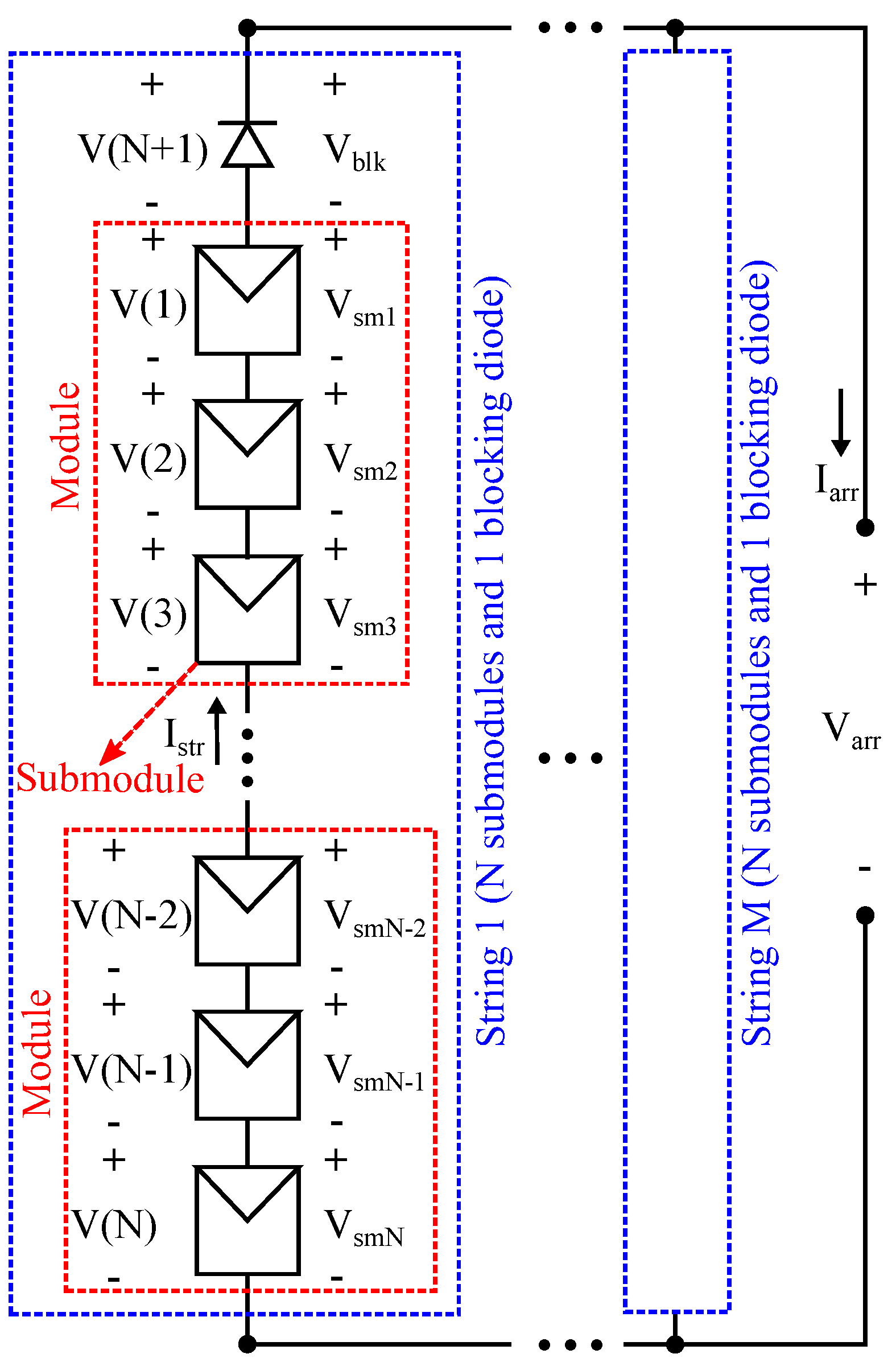
The general structure of the most widely used PV array configuration, named series-parallel (SP), is illustrated in
Figure 1. The array is formed by
M columns or strings, and each string is formed by a set of modules and a blocking diode connected in series. In turn, each module is formed by one or more series-connected submodules, where each submodule is formed by
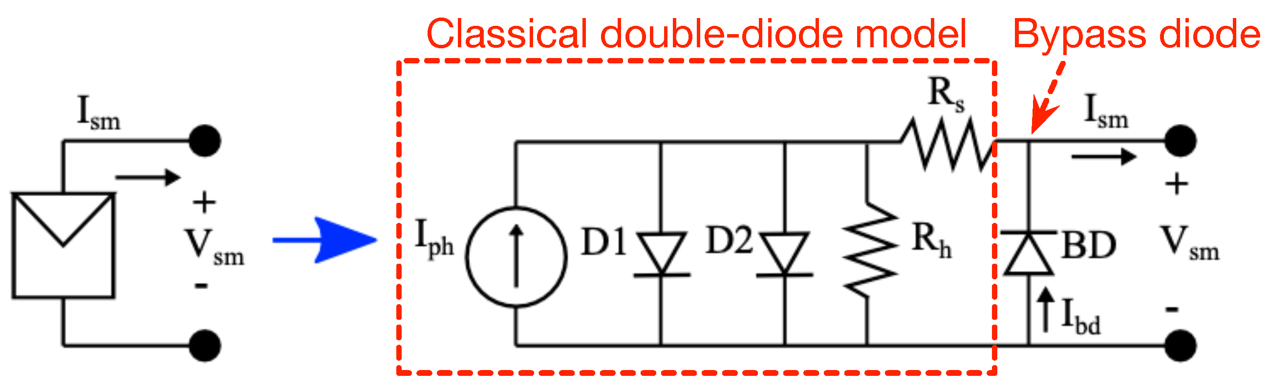
cells connected in series and a protection diode connected in anti-parallel, named bypass diode; such a submodule structure is depicted in
Figure 2, where the double diode model represents the
series-connected cells. Hence, each string of a SP array can be analyzed as a set of
N submodules and one blocking diode connected in series. It is worth noting that the array voltage (
in
Figure 1) is usually fixed by the power converter where the array is connected to; therefore, it is assumed as a known value.
This section introduces the mathematical descriptions of the main elements that form the PV array (submodules and blocking diodes) and the system of non-linear and implicit equations that describe each string, as proposed in [
23]. Moreover, this section also presents the procedure to calculate the array current by using parallel computing.
2.1. Submodule and Blocking Diodes Model
The submodule is the main element of the PV array and it is represented by using the equivalent electric circuit illustrated in
Figure 2, where the current source (
) represents the current generated by the photovoltaic effect and the diodes
and
represent the cells diffusion and recombination currents, respectively. Furthermore, the resistors
and
represent the ohmic losses and leakage currents, respectively, and the bypass diode (
) limits the power dissipation in the submodule cells when they are under partial shading conditions [
48].
The equation that relates the submodule’s current (
) and voltage (
) is shown in (
1), which is a nonlinear and implicit equation. In (
1) the parameters
and
are the inverse saturation current and ideality factor of diode
, respectively; while
,
,
and
correspond the same parameters for diodes
and
. Moreover,
is the thermal voltage of the PV cells and it is defined as
, where
k is the Boltzmann constant,
q is the electron charge,
T is the cells temperature. Additionally,
is the current through the diode
, as shown in (), and its thermal voltage is defined as
, where
is the bypass diode temperature. It is worth noting that the submodule’s parameters depend on the irradiance and temperature, which is discussed in detail in [
49].
The other key element in the SP arrays is the blocking diode, which prevent opposite current flows through the string coming from the other strings of the array. The relation between the blocking diode current (
) and voltage (
) is introduced in (
3), where
is the inverse saturation current,
is the ideality factor, and
is the thermal voltage. Furthermore,
is defined as
, where
is the blocking diode temperature.
2.2. Calculation of the String Current and Voltages
In a SP array formed by M strings connected in parallel, where each string has N submodules, i.e., an array, each string is formed by elements (N submodules and one blocking diode). Therefore, there are unknown electrical variables that correspond to: the voltages of the N submodules (), the blocking diode voltage, and the string current (), which is shared by all the elements in the string.
To calculate the
unknowns, it is necessary to define the system of
nonlinear and implicit equations given in (
4) [
23], where the first
N equations are obtained by applying (
1) for each submodule, the
equation is obtained by using (
3), and the last equation is obtained by applying KVL to the string including the array voltage. In expression (
4),
V is a vector formed by
voltages, where the first
N elements correspond to the submodules voltages from top to bottom (i.e.,
) and the last element is the blocking diode voltage with the opposite polarity (i.e.,
). Moreover,
is the string current and
is the array voltage, which is shared by all the strings and it is assumed known. The system of equations
can be solved by using a numerical method or an optimization algorithm to obtain all the electrical unknowns in the string [
50,
51]. In this paper the Trust-Region Dogleg optimization algorithm [
51] is used to solve
for each string, but any other suitable method can be adopted.
2.3. Calculation of the Array Current Using Parallel Computing
To calculate the array current it is necessary to solve (
4) for each string of the array. At that point, all the strings currents are known and the array current can be calculated by using (
5).
It is worth noting that the system of nonlinear equations of each string does not depend on the electrical variables of the other strings; hence, all the strings in an
array can be solved independently. This particular characteristic is used in this paper to reduce the model solution time by using parallel computing, since each string can be solved by a different core or processing worker. This type of parallel computation can be performed using synchronous or asynchronous algorithms [
52], where the workers in synchronous solutions wait for some synchronization condition, while the workers in asynchronous solutions can be used for other task when they finish the initial work. As it was previously described, the array current is calculated as the sum of all the strings currents; hence, that condition is an inherent synchronization point for the parallel calculation of the array current. Therefore, the solution proposed in this paper is a synchronous parallel algorithm.
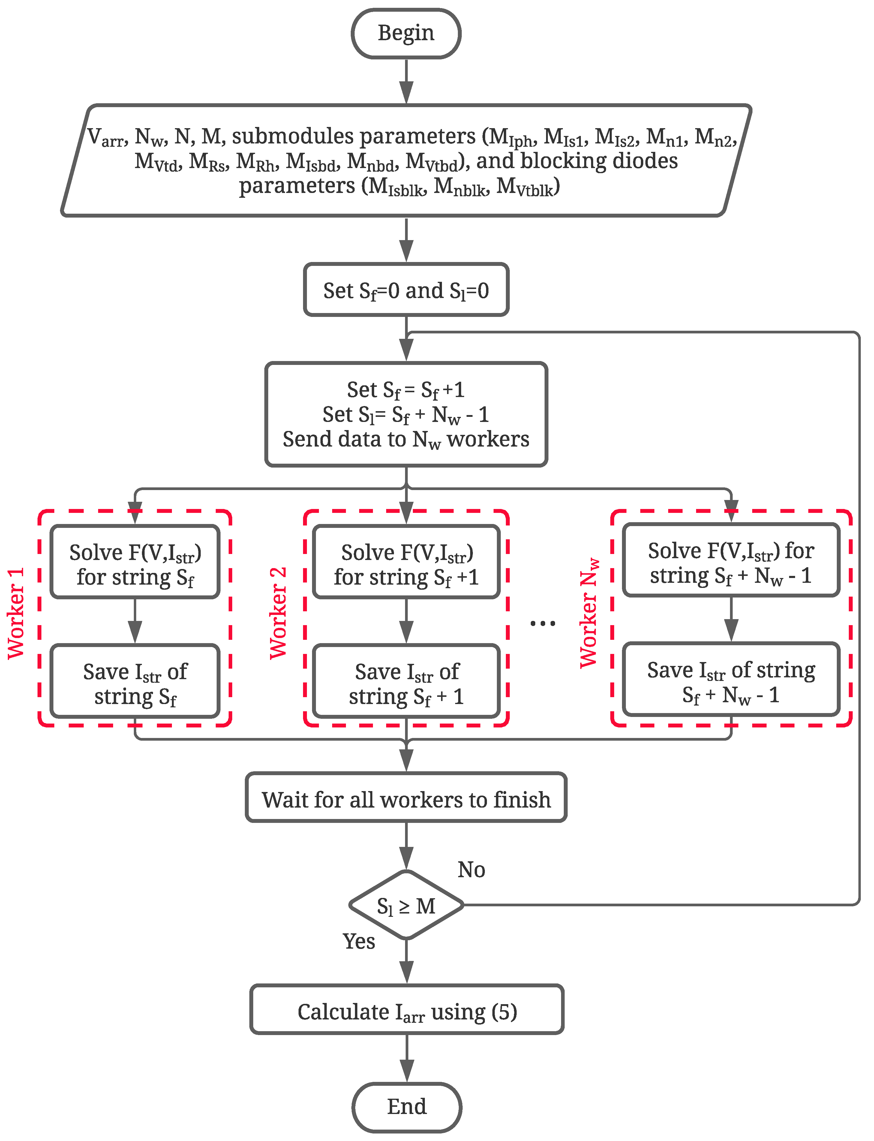
The flow chart of the proposed model to solve SP arrays using parallel computing is shown in
Figure 3, where the input data are: the array voltage (
),
N,
M, and the model parameters of all the submodules and blocking diodes. Those parameters are organized in eleven
matrices (
,
,
,
,
,
,
,
,
,
, and
), for the DDM parameters, and three
matrices for the blocking diode parameters (
,
,
). Moreover,
is the number of available workers and
and
are auxiliary variables that define the first and last string to be evaluated, respectively.
The first step is to send the data of
strings to the available workers. Then, each worker constructs the vector
V and solves the system of nonlinear and implicit equations of the corresponding string. Once the string is solved, the current is saved to calculate
later. When the
workers have solved the
strings, it is necessary to verify if all the strings has been solved; otherwise, the process is repeated until the
M strings are solved. Finally, the array current is calculated by using (
5).
At this point all the array is solved for a given value of , which can be used for different model based applications. For example, to generate the array I-V and P-V curves it is necessary to perform a voltage sweep of the array voltage from to the array open-circuit voltage and save the values of . Moreover, the proposed model can also be used to perform dynamic simulations of SP arrays in conjunction with power converters and maximum power point tracking techniques.
3. Result and Discussion
The proposed model is validated using experiments and detailed simulations, and those results are contrasted with the model proposed in [
23], which is denominated Serial model. The details of the experimental results are introduced in the corresponding
Section 3.4; hence, the following paragraphs provide information that apply for all the simulation scenarios.
This section includes, first, three evaluation scenarios to show the performance of the proposed model in terms of the errors in the I-V curve reproduction, the improvement in the calculation time for SP arrays with different number of strings, and an application example (model-based reconfiguration analysis). Moreover, all the simulations of the proposed model, from here on denominated Parallel model, are performed by using only two processing workers (i.e., ) to consider the worst case scenario for a parallel computing application. However, higher number of workers can be used depending on the computational platform.
The Trina Solar TSM-PD05 270 W module is used as a reference to construct the arrays considered in this section, whose main electrical characteristics in standard test conditions (STC) are: short-circuit current 9.22 A, open-circuit voltage 37.9 V, Maximum Power Point (MPP) current 8.73 A, MPP voltage 30.9 V, shot-circuit current temperature coefficient 0.05 %/K, open-circuit voltage temperature coefficient −0.32 %/K, number of cells 60, and number of submodules 3; therefore, each submodule has 20 cells (i.e.,
). From those characteristics, and considering an irradiance of 1 kW/m
(
kW/m
) and a cell temperature of 55
C (
K), it is possible to calculate the following DDM parameters, of each submodule, by using the procedure proposed in [
53]:
A,
A,
A,
,
,
,
. Moreover, the parameters of both bypass and blocking diodes models are calculated from the GF3045T bypass diode datasheet information, obtaining
A, and
.
For sake of simplicity, it is assumed that all the submodules and blocking diodes have the same parameters, and also it is considered that the cells, bypass diodes, and blocking diodes operate at almost the same temperature (i.e.,
) [
47,
54]. In any case, under experimental conditions, each parameter can be calculated independently using the procedure reported in [
55,
56]. Finally, the partial shading conditions are defined by using the matrix
, since
is directly proportional to the irradiance reaching each submodule [
57].
3.1. Error Evaluation under Different Partial Shading Conditions
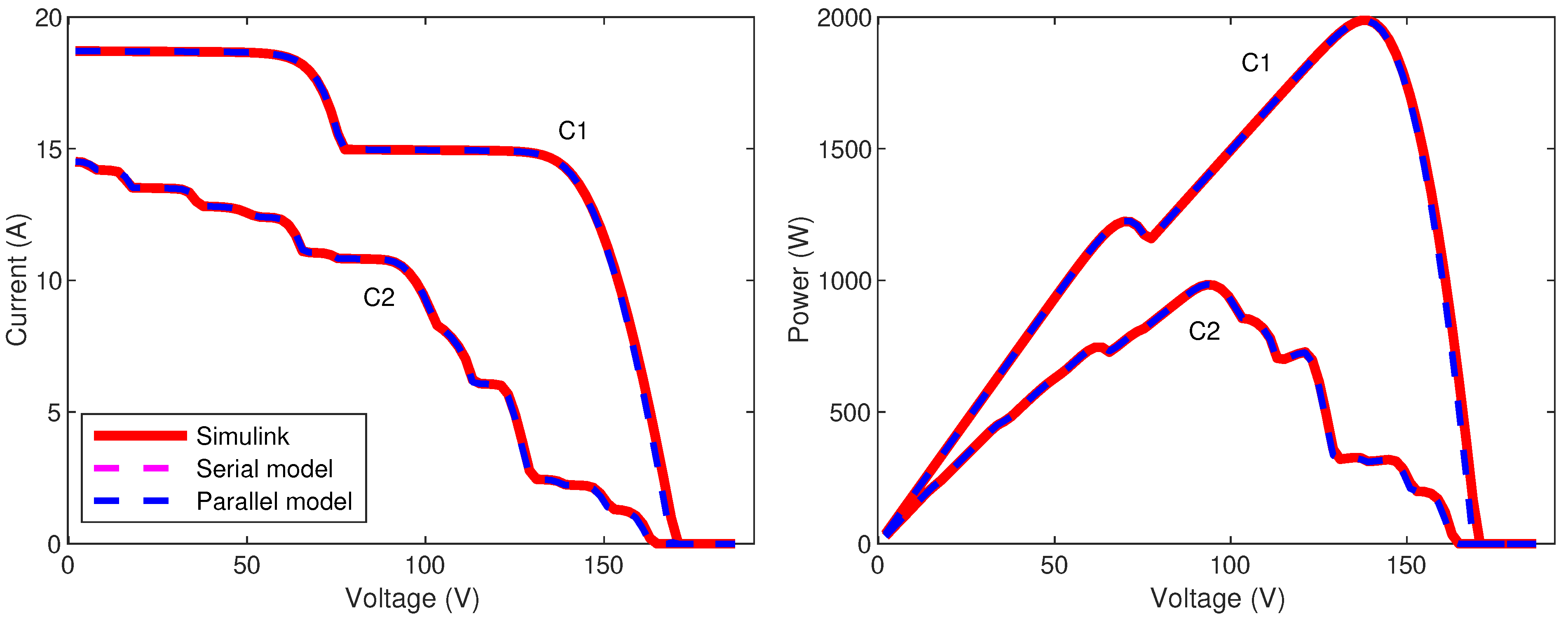
This analysis considers a (i.e., and ) array with two partial shading conditions ( and ) to evaluate the errors in the current prediction of both the Series and Parallel models regarding the array equivalent circuit implemented in Simulink. Condition represents a shading profile with two irradiance levels ( kW/m and kW/m), while represents a random shading condition with submodule irradiance varying from kW/m to kW/m.
The I-V and P-V curves of the SP array, for operating conditions
and
, are introduced in
Figure 4, where the Simulink results are plotted in red lines, while Serial and Parallel models are plotted in magenta and blue discontinuous lines, respectively. As expected, Serial and Parallel models provide the same results for both operating conditions, since the blue dashed line is over the magenta dashed line.
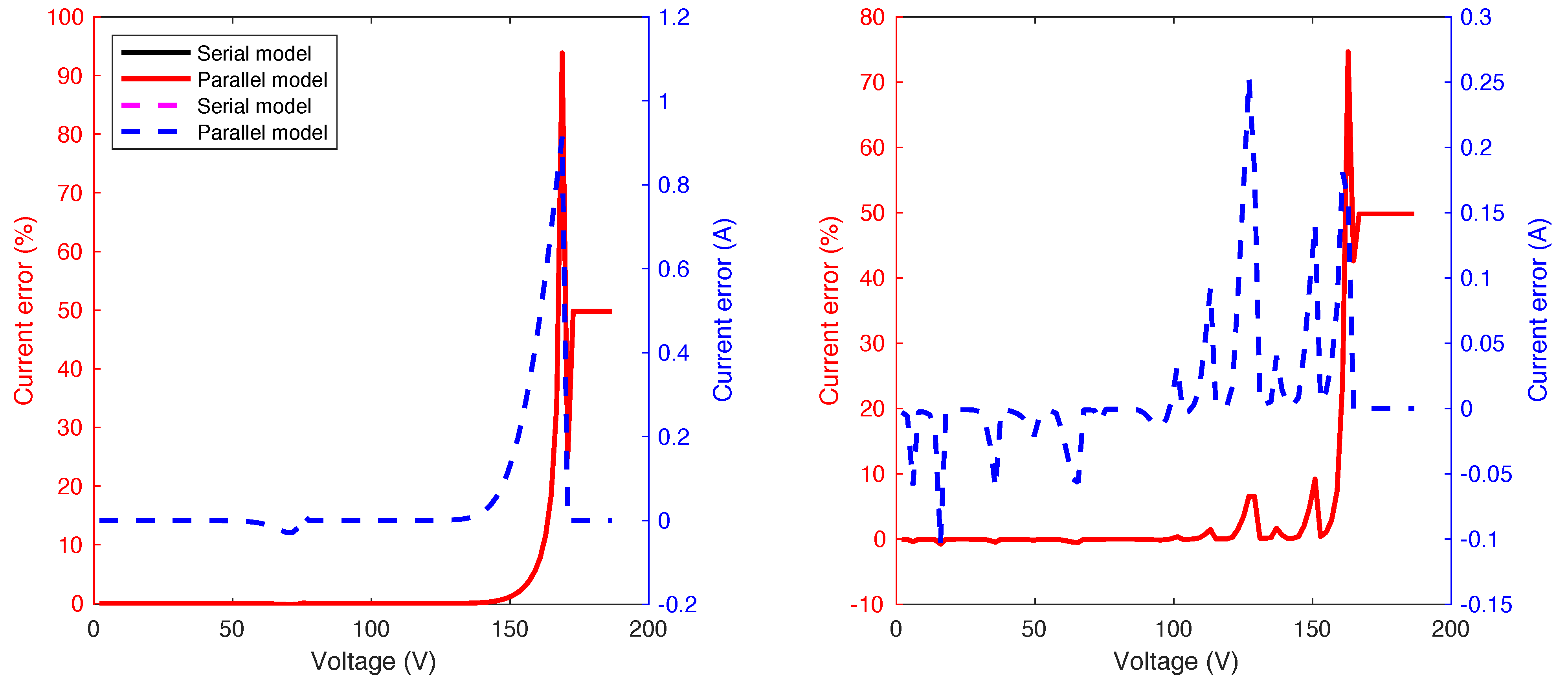
The errors in the current calculation of the Series and Parallel models are shown in
Figure 5. As expected, the errors obtained with the two models are exactly the same, since both models solve the same systems of equations with the same algorithm; hence, both models provide the same Normalized Sum of Squared Errors (NSSE) for both operating conditions: 0.0139% for
and 0.0032% for
. In the left plot of
Figure 5, it can be observed that the largest errors for condition
are close to the open-circuit voltage (169 V) and the inflection point (71 V), where the errors are
A (+93%) and −29.2 mA (−0.17%), respectively. Around those points the derivative of the current with respect to the voltage increases; therefore, the small differences between the equivalent array circuit and the models are translated into increments in the current errors. Additionally, it is important to mention that the high percentage in the current error close to the open-circuit voltage is expected since in this region of the I-V curve the currents are close to 0 A. Nevertheless, those current errors do not considerably affect the I-V curve reproduction, as observed in
Figure 4. The increment of the current errors around the inflection points of the I-V curve is also evidenced in the right plot of
Figure 5 for condition
. In such a plot each increment in the magnitude of the current error corresponds to an inflection point in the I-V curve; however, those errors do not affect significantly the I-V reproduction. Moreover, for condition
the errors move from −0.103 A (−0.75%) close to 16 V to +0.253 A (6.53%) close to 127 V; while the largest percentage error is again close to the open-circuit voltage (163 V) with 0.160 A (74.6%).
3.2. Calculation Time for Different Number of Strings
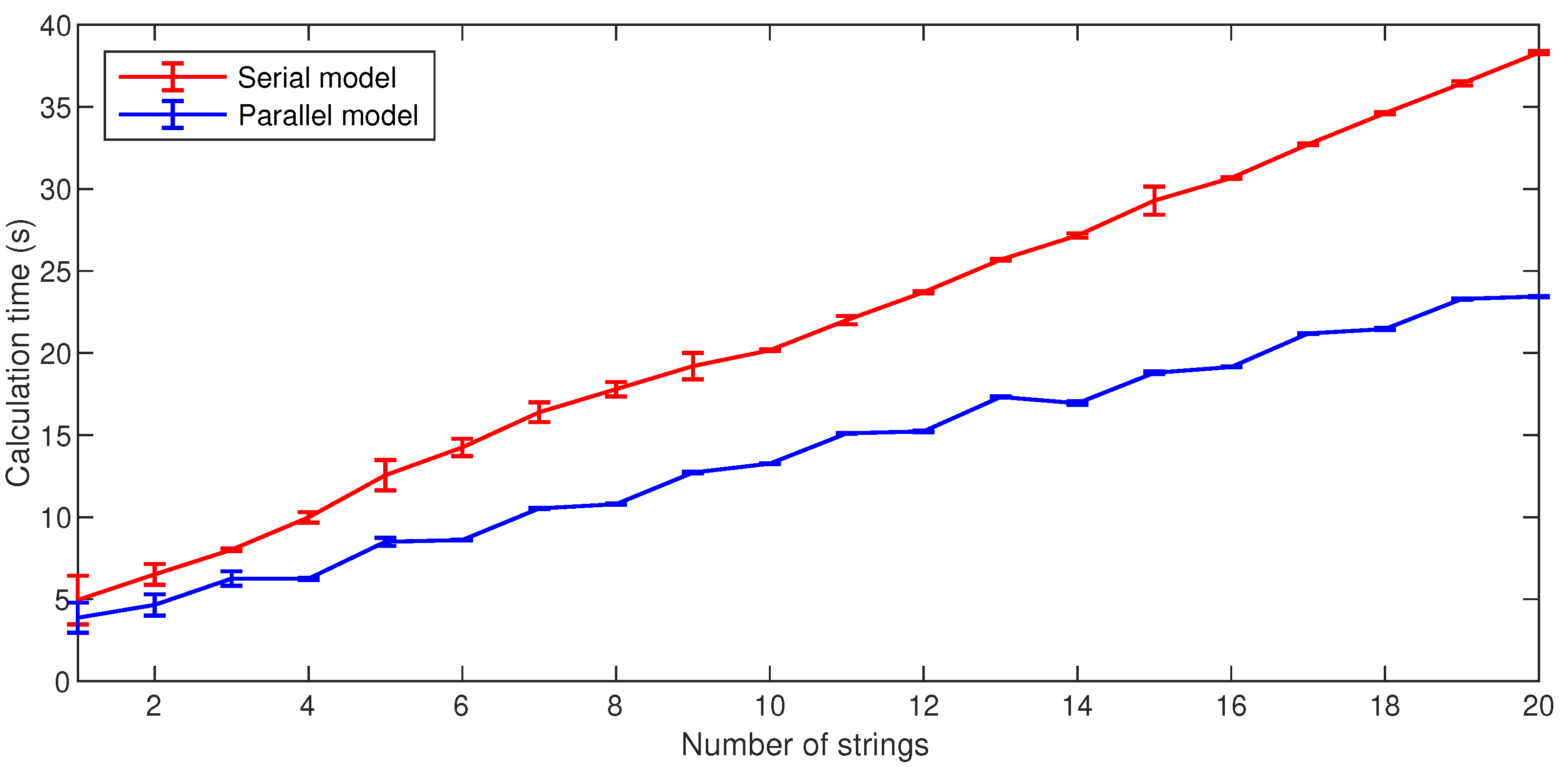
The main advantage of the Parallel model is the reduction of the calculation time without sacrificing the solution accuracy. Hence, the analysis performed in this section evaluates the calculation time of both Series and Parallel models to generate the I-V curve for a SP array with fifteen rows (), and the number of columns varying from one to twenty (i.e., ). All the I-V curves are generated with voltage steps of 2 V in , and each I-V curve is calculated six times to evaluate the average computation time and standard deviation for each array. In addition, the shading profiles for all the strings are randomly generated to represent a complex partial shading condition with a high number of inflection points in the I-V curves.
Figure 6 shows the calculation time and standard deviation of the I-V curves for both Serial and Parallel models considering SP arrays from
to
. It is worth noting that those results are obtained with two processing workers (i.e.,
) for the Parallel model, which is the worst case scenario regarding the number of workers. Moreover, the exact mean values and standard deviations are presented in
Table 1 as well as the average time reduction obtained with the Parallel model and its standard deviation.
For arrays with from 1 to 3 the calculation times are close but there is a reduction below between 2.5% and 28.0% with the Parallel model. Then, the calculation time of both models increases linearly regarding the number of strings in the array. However, the calculation time of the Serial model increases with a higher slope (1.73 s/string) than the one of the Parallel model (1.058 s/string). Hence, in general, the proposed model reduces the calculation time between 20.6% and 39.5% with respect to the Serial model with an average standard deviation of 2.13%. Furthermore, the standard deviations of the calculation times of both models confirm their repeatability.
3.3. Application Example: Exhaustive Model-Based Reconfiguration
The reduction in the calculation time provided by the Parallel model is useful in model-based reconfiguration systems. In those applications, the I-V curves must be calculated as fast as possible to reduce the reconfiguration time (period), since the shorter the reconfiguration period, the higher the power generation under partial shading conditions [
58,
59]. This is due to the continuous change in the shading profiles generated by the movements of the sun in the sky along the day and year.
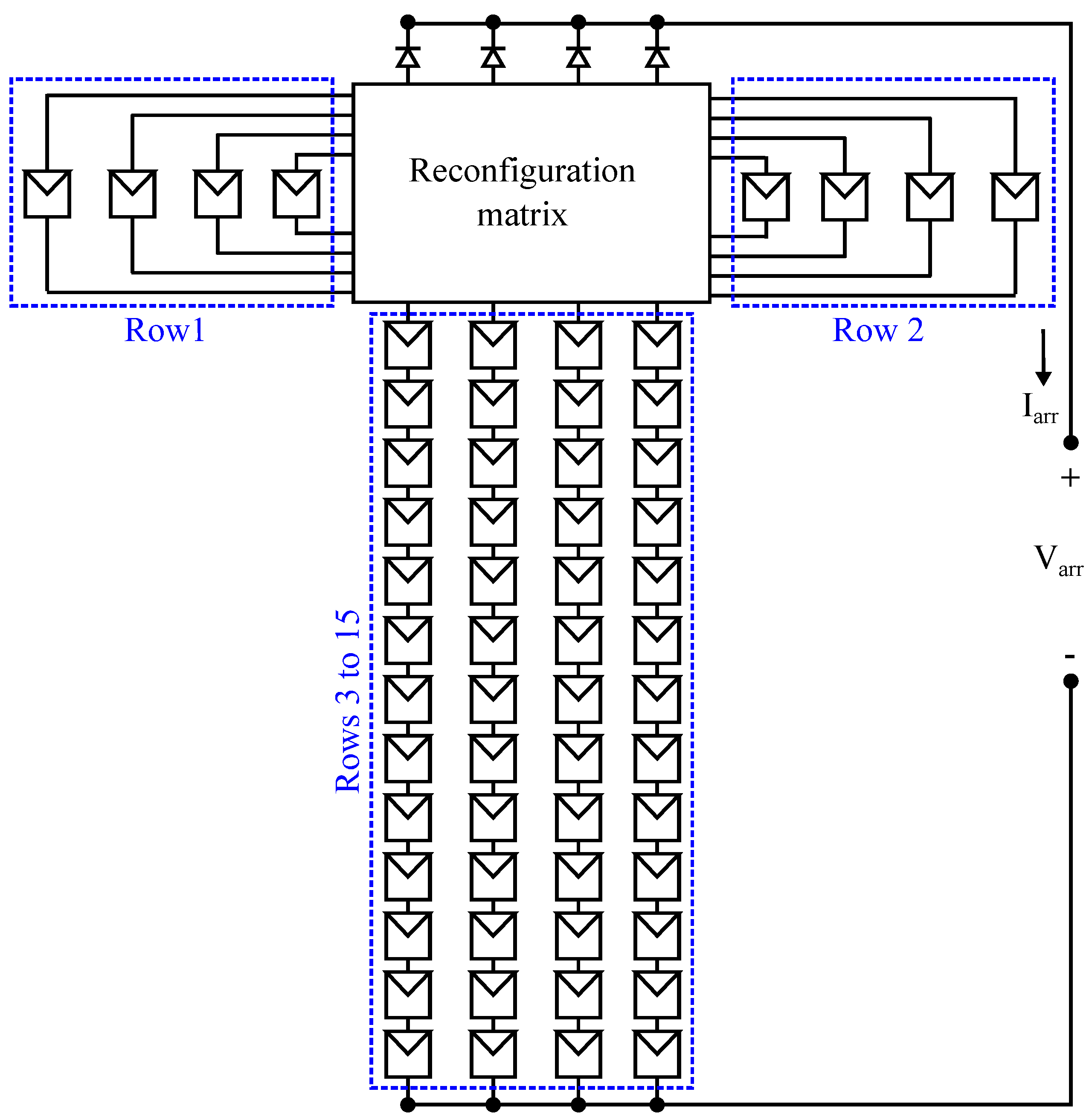
The reconfigurable array considered in this application example is illustrated in
Figure 7, which is a
array where the first two rows are reconfigurable (i.e.,
) and the rest of the array is fixed (i.e.,
). The eight reconfigurable submodules can be connected to any string through the reconfiguration matrix, which is implemented with switches (e.g., relays or MOSFETs) and controlled by the reconfiguration algorithm. This type of systems with a fixed and a reconfigurable parts have been previously reported in the literature because, sometimes, only part of the array is affected by partial shading conditions [
60].
In this example, it is assumed that the reconfiguration algorithm evaluates all the possible configurations, i.e., it performs an exhaustive search. For the array explained before, it is possible to construct 105 different configurations with the eight reconfigurable submodules and the reconfiguration matrix. For each configuration the model generates the P-V curve, with voltage steps of 2 V, to identify the global maximum power point (GMPP). Then, the GMPP of each configuration is saved to determine the one that provides the highest GMPP. Once the best configuration is identified, the reconfiguration algorithm sets the reconfiguration matrix to implement such a best configuration into the PV array.
The analysis is performed for three different shading profiles defined through the
matrix. The values of
for the reconfigurable part are reported in
Table 2, while the values of
for the fixed part of the array are defined as follows: 5.6150 A for rows 3 to 9 (i.e.,
A
) and 2.8075 A for rows 10 to 15 (i.e.,
A
).
The 105 possible configuration were evaluated six times for each shading profile, with both the Serial and Parallel models, in order to calculate the average processing time values and the standard deviations shown in
Table 3. The average time required by the Serial and Parallel models to evaluate the 105 configurations are 719.96 s (or 11.99 min) and
(or 8.64 min), respectively, which implies a time reduction between 26.6% and 29.3% (with standard deviations lower than 0.23%) in the reconfiguration algorithm period when the Parallel model is used. Such a reduction indicates that the reconfiguration system using the Parallel model is able to enhance the array power production under mismatching conditions. Once again, it is important to highlight that these results were obtained with two processing workers (
); hence, the calculation time can be further reduced by using as many workers as strings in the array (i.e.,
).
In addition, in this application example the improvement in the maximum power extracted, comparing the best and worst configurations, varies from 7.39% for shading profile 1 to 4.36% for shading profile 3 (see
Table 3). This indicates that the increment in the power production obtained by a reconfiguration system depends on the shading profile; however, such increment is translated into a higher energy production, a reduction in the project’s payback time, and a mitigation of the power generation variability of PV generators.
3.4. Experimental Results
The proposed model is also validated with experimental results for a
array formed by three modules Trina Solar TSM-PD05 270W connected in parallel, where each module has three series-connected submodules. The I-V curves of each string and the array are measured with a BK Precision electronic load, which is controlled from a PC through serial communication. The parameters of the DDM parameters used for the experimental validation are introduced in
Table 4 and
Table 5, where the first one shows the
values for each submodule, while the second table presents the rest of the DDM parameters. It is worth highlighting that the parameters of the three submodules in one string are assumed equal; that is why
Table 5 shows one DDM parameter for each string.
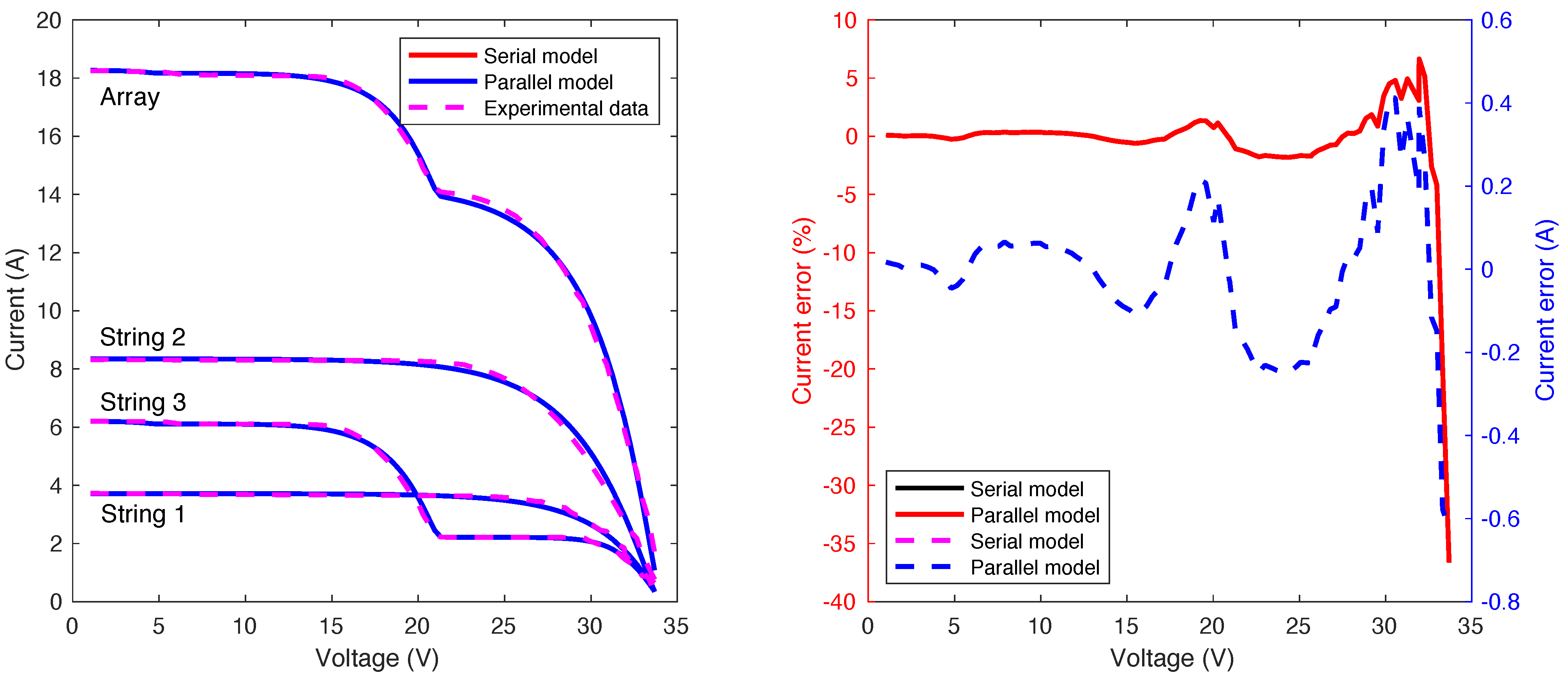
Serial and Parallel models are used to reproduce the experimental results. The I-V curves of each string and the array are introduced in the left plot of
Figure 8; while the error in the estimation of the array current is presented in the right plot of
Figure 8. As in the previous examples, the results obtained with both models are the same, which entails the same errors. Moreover, the error varies from −0.62 A (−36.64%) to
A (+4.79%), where the highest values of the errors are obtained close to the open-circuit voltage, as in the simulation results. However, both models correctly reproduce the electrical behavior of the PV array according to the results shown in
Figure 8 and the NSSE obtained for both models (
0.012%).
Additionally, Serial and Parallel (with ) models are executed six times to validate the repeatability of the results obtaining that the average time required by the Serial and Parallel models are 2.1464 s and 2.0908 s. Hence, in this case, the time improvement obtained with the Parallel model is relatively low (2.590%), which is expected considering the low number of strings and rows in the array.
Finally, the simulation and experimental results introduced in this section show the applicability of the proposed model and the consistent time reduction obtained in different evaluating scenarios.
4. Conclusions
This paper has presented a parallel modeling strategy for SP arrays, which can reduce the processing time required to calculate the power production of the array without impacting the solution accuracy. This parallel solution is based on the double-diode model, it providing a higher accuracy in comparison with the classical single-diode model at low voltage and low irradiance conditions, which are important for partial shading analysis. Therefore, this solution is very useful for reconfiguration systems, since the parallel model will enable a fast modification of the array connections to improve the power production, and such a reconfiguration will be based on accurate predictions.
The previous claims were tested in several scenarios. The first test demonstrated the high accuracy of the parallel model since the prediction errors were very low in comparison with a commercial solution based on Simulink. The second test demonstrated that the proposed parallel model significantly improves the calculation speed over the classical serial model, which in this case reaches 40%; however, the calculation speed can be further improved by increasing the number of workers used to parallelize the calculation process. The third test demonstrated the applicability of the parallel model to reconfiguration systems, where the calculation speed was significantly improved, thus enabling the reduction of the reconfiguration period. Therefore, the PV array can be reconfigured more times during the day, which enables the optimization of the array connections to more partial shading conditions; hence, more power can be generated from the same reconfigurable array. The final test, based on experiments made on commercial PV panels, confirmed the model accuracy for real-world applications.
Another possible application for this parallel solution concerns the estimation of the potential power production of PV plants, which can be subjected to partial shading during some hours of the day (caused by seasons or unavoidable obstacles). This is critical for the economic viability analysis of PV plants, since partial shading could significantly decrease the power production; hence, the lifetime production of the PV plant is a decisive factor to consider. However, estimating the power production of a partially-shaded PV array requires a lot of calculations (and time), thus the proposed parallel solution could significantly reduce the processing time required. Such a fast calculation could enable to test much more possible installation sites and architectures since each test will take less time.
The main disadvantage of the parallel model is the requirement of multiple cores or workers, which is not needed to implement the classical serial model. However, processors available inside commercial computers have multiple cores (4, 6, 8, and more), thus the parallel model can take advantage of that hardware, which is neglected by the serial model. Another scenario concerns the embedded implementation adopted for real-time applications, which usually provide a single core; in any case, newer SoCs provide multiple cores [
44], hence the parallel model can be implemented in embedded applications using those newer devices. Of course, multi-core embedded systems are costly in comparison with single-core devices, but the increased power production provided by the parallel model in reconfiguration systems, under partial shading conditions, could justify the increased cost of the embedded system. Otherwise, in the cases when the power increment is not enough, the serial solution will be more profitable; thus, an economic viability analysis is mandatory.

 ,
, 


