
A Multiobjective Variable Neighborhood Strategy Adaptive Search to Optimize the Dynamic EMS Location–Allocation Problem

 ,
,  ,
,  ,
,  ,
,  ,
, 
Abstract
:1. Introduction
1.1. Motivation
1.2. Related Works
1.3. Contribution
- The assignment of the trained medical volunteer (TV) is first integrated into the EMS location problem. Due to the limitation of medical staff during a pandemic, a shortage of medical staff occurs; hence, a TV is used as a substitute for the medical staff; however, the levels of TVs’ experience are different. If the TV’s assignment is not suitable, it can affect the ability of the EMS to rescue the patients, which is the main concern of this article.
- The IOT is used to collect the real average speed of a car along a particular road obtained from speed checkpoints. The IOT’s device submits this information to the EMS center, the data are analyzed, and real-time location information is sent to the EMS. This can help the EMS to reach the patients within the PST.
- A new black box (improvement box) selection formula is first presented to improve the search performance of the original VaNSAS. A multiobjective variable neighborhood strategy adaptive Search (M-VaNSAS) is presented in this paper, and it is evaluated in comparison to existing well-known metaheuristics.
2. Mathematical Model Formulation
- Indices
- i: EMS i (i = 1,2,3,…,I)
- l: Trained volunteer (TV)
- k = 1,2,3,…,K
- j: Community j (j = 1,2,3,..,J)
- t: Time period t (t = 1,2,3,..,T)
- Parameters
- I: Number of EMSs
- J: Number of communities
- H: Maximum traveling time from the EMS to the community
- R1: EST time
- R2: PST time
- El: Experience level of TV l
- Tijt: Traveling time per kilometer from i to j at time t (min)
- L: Number of trained volunteers
- T: Length of planning period
- O: Maximum communities that an EMS can serve
- M: Minimum level of experience in an EMS
- Cl: Cost of TV l (THB)
- D: Maximum number of TVs in one EMS
- Ai: Capacity of EMS i
- Pjt: Size of population in j time t
- B: Traveling cost per min of an EMS
- Decision Variables
- Objective Functions
- Subject To
3. The Proposed Method
3.1. Generate the Initial Tracks
- The Decoding Method
- Trained Volunteer Assignment Procedure
3.2. Perform Track Touring Process
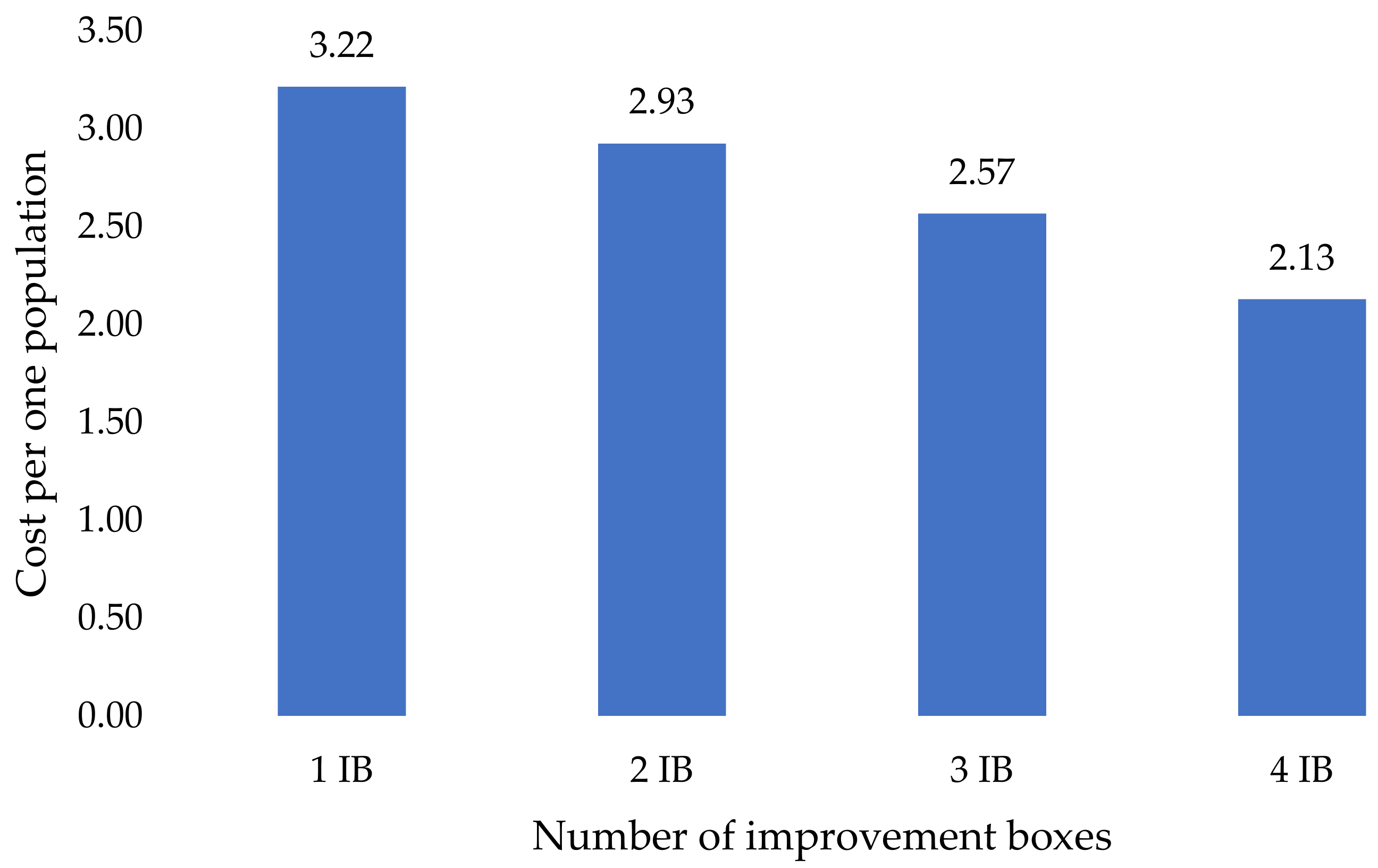
3.3. Update the Probability of the Black Box (IB)
3.4. Repeat Steps 3.2–3.3
| Algorithm 1: Multiobjective variable neighborhood strategy adaptive search (M-VaNSAS)-EMS | |
| 1 2 3 4 5 6 7 8 9 10 11 12 13 14 15 16 17 18 19 20 21 22 23 24 25 26 27 28 29 30 | Input: Number of tracks (NT), Number of parameters (D), Scaling factor (F), Improvement factor (K), Value of CR, Number of improvement box (IBPop) Output: Best_Track_Solution Begin Population = Initialize Population (NT, D) IBPop = Initialize InformationIB (NIB) Encode Population to WP while the stopping criterion is not met do for i = 1: NT //selected improvement box by roulette wheel selection selected_IB = RouletteWheelSelection(IBPop) if(selected_IB = 1) Then new_u = RT (u) Perform RT else if(selected_IB = 2) new_u = BT (u) Perform BT else if(selected_IB = 3) new_u = IT (u) Perform IT else if(selected_IB = 4) new_u = SF(u) Perform SF Perform Decoding method, Weight Sum Method if(CostFunction(new_u) ≤ CostFunction(Vi)) Then Vi = new_u Update Pareto Front End for loop //end update heuristics information End while loop End |
3.5. Comparison Methods
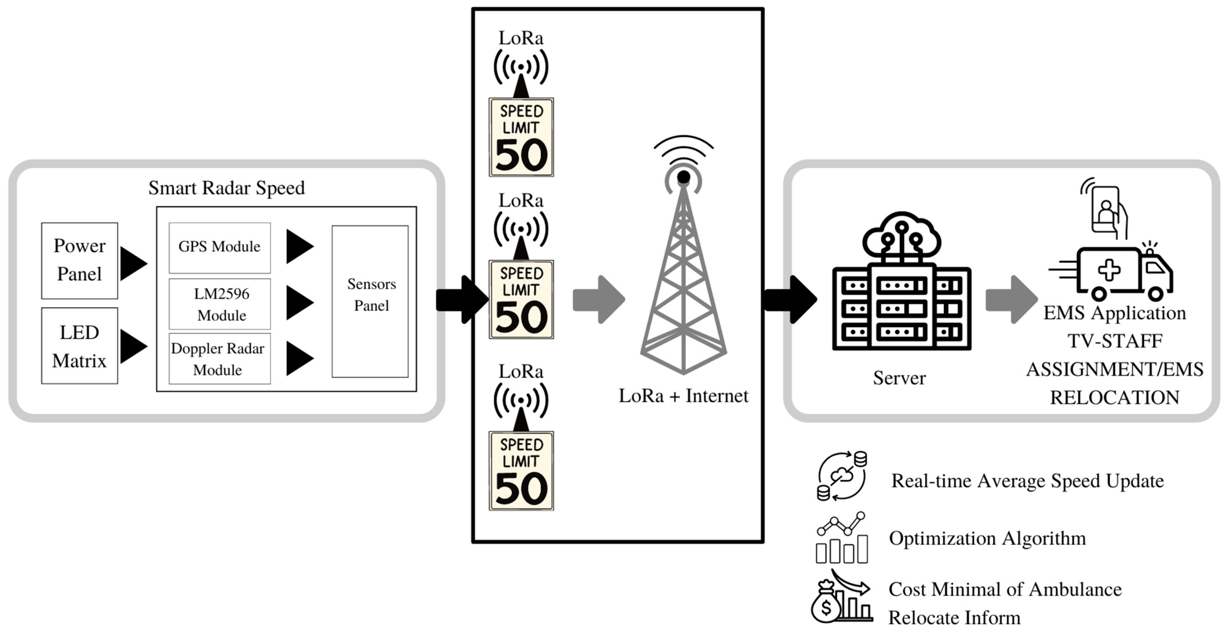
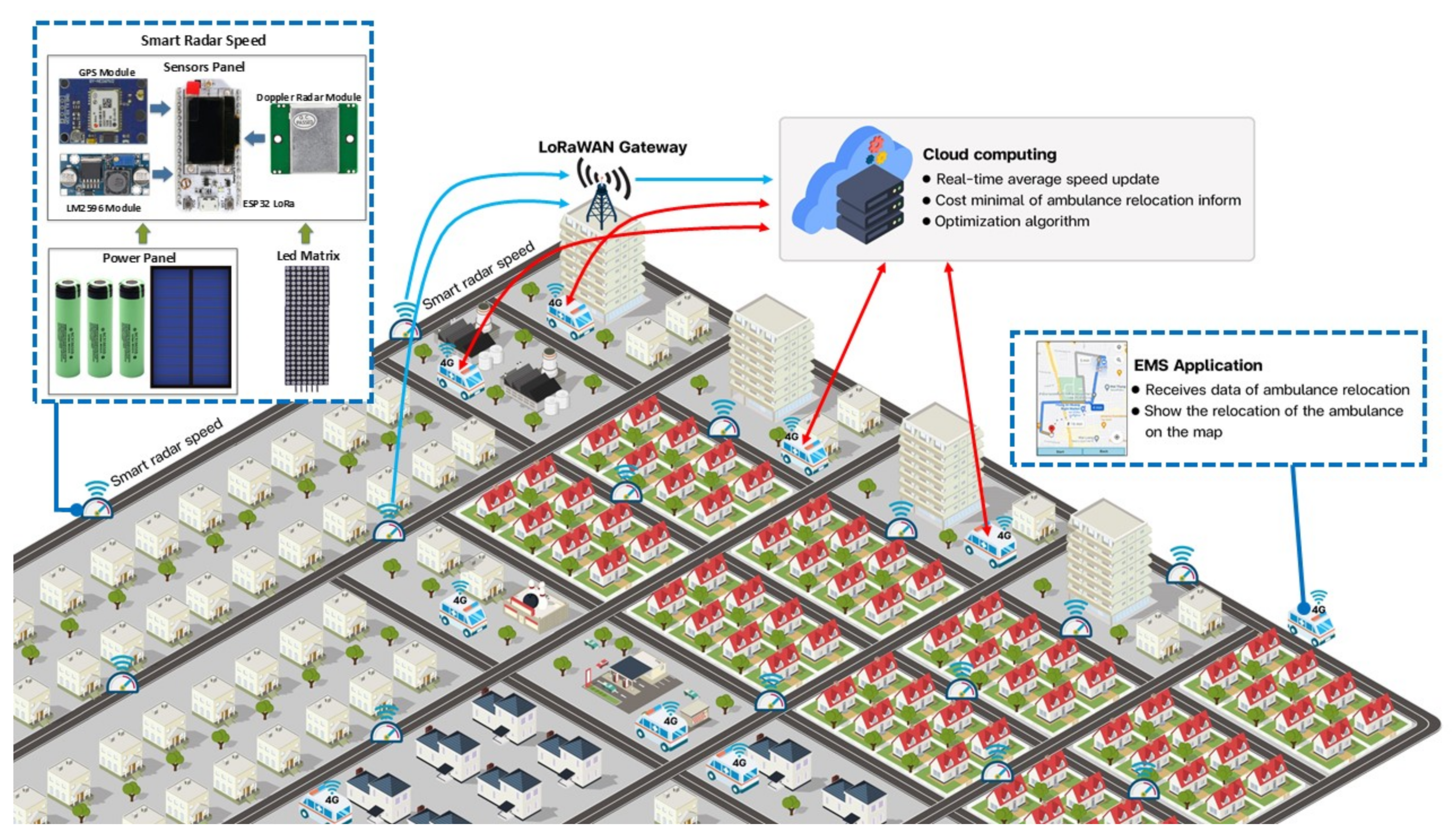
3.6. IOT and Mobile Application Architecture Design
- The smart radar speed consists of six components: an ESP32 LoRa, a GPS module, a Doppler radar module, an LM2596 module, a power panel, and an LED matrix. The Doppler radar module, GPS module, and LED matrix were connected to a printed circuit board; the core of the board is an ESP32 LoRa microcontroller, which has a 32-bit CPU operating at 160 MHz, with 16 MB of ROM and 512 KB of RAM, and the integrated LoRaWAN communication in the 920–925 MHz band [35]. The circuit board used the power from a 12 V lithium−ion rechargeable battery with a solar cell. The LM2596 module was used to generate 5 V of power for the circuit board. Furthermore, the LED matrix displays the car speed obtained from the Doppler radar module.
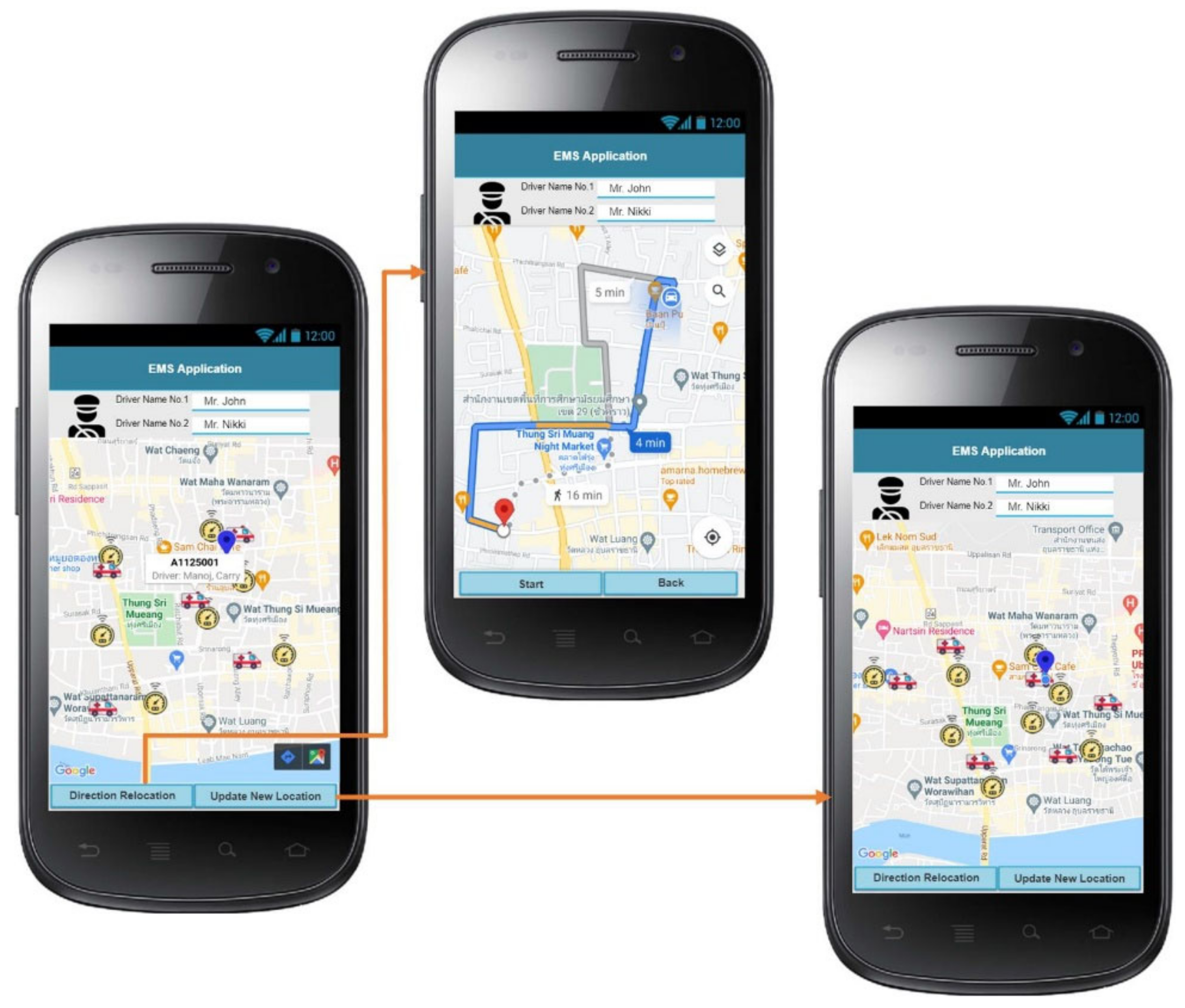
- The EMS application, shown in Figure 3, runs on the Android platform. The EMS application needs to connect to 4G, with authentication via a login; then, the application obtains the data from the server’s database and displays them on the screen of the application. A Google Maps API displays the current location and journey of the ambulance on the application. Furthermore, the EMS application provides navigation when the system notifies the ambulance to relocate.
- The server system performs the average speed calculation for each road and the lowest cost of the ambulance rerouting using an optimization algorithm; then, the server relays the ambulance relocation information to the EMS application.
- (1)
- Assign the TV to the EMS using M-VaNSAS algorithm.
- (2)
- Use current traffic condition to locate the EMS in the relevant location using M-VaNSAS algorithm.
- (3)
- Update real-time traffic situation using IOT and mobile application.
- (4)
- Reroute the EMS using M-VaNSAS algorithm.
- (5)
- Send the new location to the driver of EMS, leading back to step 1 (if needed).
- (6)
- Redo steps (3)–(5) at least every 3 h.
4. Computational Results and Framework
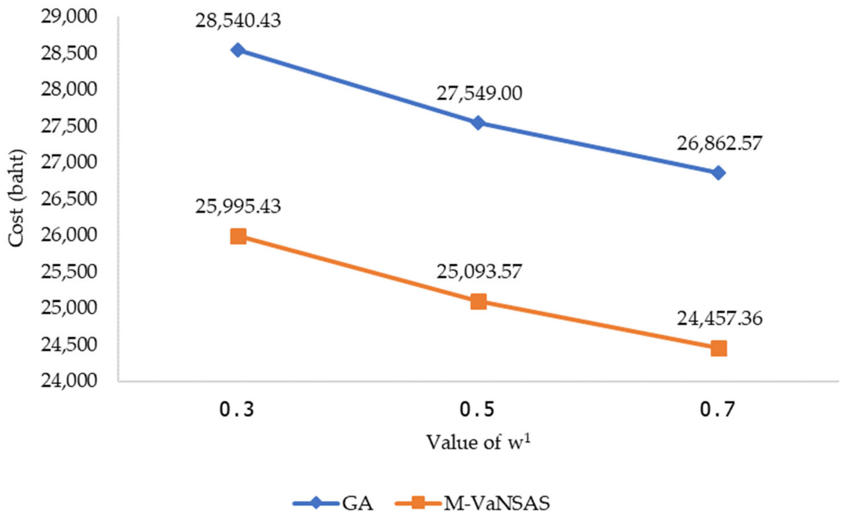
4.1. Compare the Proposed Method (M-VaNSAS) with the Results from the Optimization Software (Lingo v.16) and the Genetic Algorithm
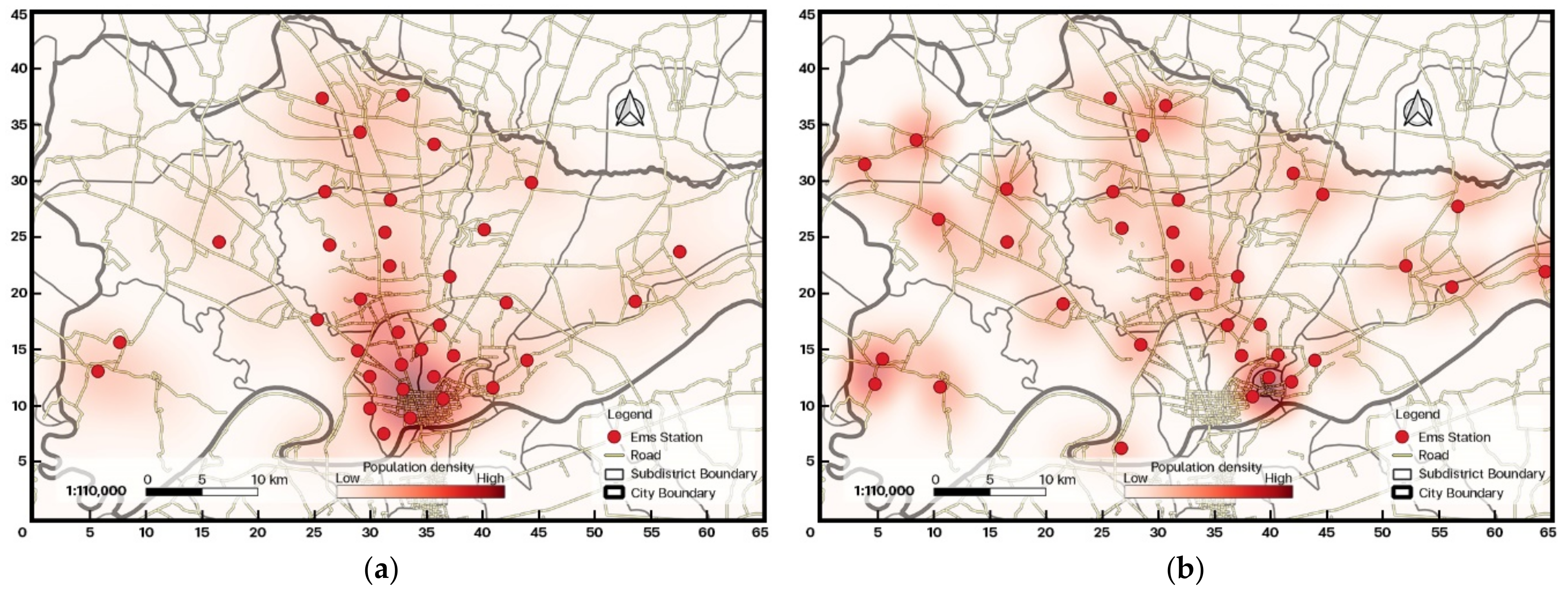
4.2. Case Study Results Compared with the Current Method
5. Conclusions and Future Outlook
- (1)
- The service time (average time to reach the patients) was reduced because of the application and IOT system designed and used in this study. Real-time traffic reporting to the central computer was used to reroute the ambulance; therefore, the EMS could reach patients more quickly.
- (2)
- The total cost and distance to service the patients were reduced due to the effectiveness of the designed algorithm (M-VaNSAS).
- (3)
- The service level of the patients was increased, as the number of people covered within seven minutes increased with M-VaNSAS; this could reduce the number of severe cases.
Author Contributions
Funding
Institutional Review Board Statement
Informed Consent Statement
Acknowledgments
Conflicts of Interest
References
- Trujillo, L.; Álvarez-Hernández, G.; Maldonado, Y.; Vera, C. Comparative Analysis of Relocation Strategies for Ambulances in the City of Tijuana, Mexico. Comput. Biol. Med. 2020, 116, 103567. [Google Scholar] [CrossRef] [PubMed]
- Bélanger, E.; Ahmed, T.; Vafaei, A.; Curcio, C.L.; Phillips, S.P.; Zunzunegui, M.V. Sources of Social Support Associated with Health and Quality of Life: A Cross-Sectional Study among Canadian and Latin American Older Adults. BMJ Open 2016, 6, e011503. [Google Scholar] [CrossRef] [PubMed] [Green Version]
- Nair, R.; Miller-Hooks, E. Evaluation of Relocation Strategies for Emergency Medical Service Vehicles. Transp. Res. Rec. 2009, 2137, 63–73. [Google Scholar] [CrossRef]
- Gendreau, M.; Laporte, G.; Semet, F. A Dynamic Model and Parallel Tabu Search Heuristic for Real-Time Ambulance Relocation. Parallel Comput. 2001, 27, 1641–1653. [Google Scholar] [CrossRef] [Green Version]
- Zidi, I.; Al-Omani, M.; Aldhafeeri, K. A New Approach Based on the Hybridization of Simulated Annealing Algorithm and Tabu Search to Solve the Static Ambulance Routing Problem. Procedia Comput. Sci. 2019, 159, 1216–1228. [Google Scholar] [CrossRef]
- Bélanger, V.; Lanzarone, E.; Nicoletta, V.; Ruiz, A.; Soriano, P. A Recursive Simulation-Optimization Framework for the Ambulance Location and Dispatching Problem. Eur. J. Oper. Res. 2020, 286, 713–725. [Google Scholar] [CrossRef]
- Mouhcine, E.; Karouani, Y.; Mansouri, K.; Mohamed, Y. Toward a Distributed Strategy for Emergency Ambulance Routing Problem. In Proceedings of the 2018 4th International Conference on Optimization and Applications (ICOA), Mohammedia, Morocco, 26–27 April 2018; pp. 1–4. [Google Scholar] [CrossRef]
- Schmid, V.; Doerner, K.F. Ambulance Location and Relocation Problems with Time-Dependent Travel Times. Eur. J. Oper. Res. 2010, 207, 1293–1303. [Google Scholar] [CrossRef] [Green Version]
- Rajagopalan, H.K.; Saydam, C.; Xiao, J. A Multiperiod Set Covering Location Model for Dynamic Redeployment of Ambulances. Comput. Oper. Res. 2008, 35, 814–826. [Google Scholar] [CrossRef]
- Chumachenko, D.; Meniailov, I.; Bazilevych, K.; Chumachenko, T.; Yakovlev, S. Investigation of Statistical Machine Learning Models for COVID-19 Epidemic Process Simulation: Random Forest, K-Nearest Neighbors, Gradient Boosting. Computation 2022, 10, 86. [Google Scholar] [CrossRef]
- Ma, X.; Zhao, X.; Guo, P. Cope with the COVID-19 Pandemic: Dynamic Bed Allocation and Patient Subsidization in a Public Healthcare System. Int. J. Prod. Econ. 2022, 243, 108320. [Google Scholar] [CrossRef]
- Yuk-Chiu Yip, J. Healthcare Resource Allocation in the COVID-19 Pandemic: Ethical Considerations from the Perspective of Distributive Justice within Public Health. Public Heal. Pract. 2021, 2, 100111. [Google Scholar] [CrossRef]
- Biswas, R.; Arya, S.; Arya, K. A Quantifiable Framework for ‘COVID-19 Exposure’ to Support the Vaccine Prioritization and Resource Allocation for Resource-Constraint Societies. Urban Gov. 2021, 1, 23–29. [Google Scholar] [CrossRef]
- Kim, D.; Pekgün, P.; Yildirim, İ.; Keskinocak, P. Resource Allocation for Different Types of Vaccines against COVID-19: Tradeoffs and Synergies between Efficacy and Reach. Vaccine 2021, 39, 6876–6882. [Google Scholar] [CrossRef]
- Chen, P.S.; Lin, Y.J.; Peng, N.C. A Two-Stage Method to Determine the Allocation and Scheduling of Medical Staff in Uncertain Environments. Comput. Ind. Eng. 2016, 99, 174–188. [Google Scholar] [CrossRef]
- Vieira, B.; Demirtas, D.; van de Kamer, J.B.; Hans, E.W.; van Harten, W. A Mathematical Programming Model for Optimizing the Staff Allocation in Radiotherapy under Uncertain Demand. Eur. J. Oper. Res. 2018, 270, 709–722. [Google Scholar] [CrossRef] [Green Version]
- Evoy, K.E.; Raber, H.P.; Battjes, E.N.; Sheridan, E.P. Volunteering as Medical Staff at a Diabetes Summer Camp as a Component of a Pharmacy Residency Program. Curr. Pharm. Teach. Learn. 2016, 8, 437–441. [Google Scholar] [CrossRef]
- Wise, D.; Bruun, T.; Swee, J.; Caceres, W.; Singh, B.; Ahmed, A. Sa1516 Linkage-to-Care for Patients with Viral Hepatitis Provided by the Free Community-Based Hepatology Clinic Organized by Medical Students and Staffed by Volunteer Hepatologists. Gastroenterology 2020, 158, S-1318. [Google Scholar] [CrossRef]
- Chow, C.; Goh, S.K.; Tan, C.S.G.; Wu, H.K.; Shahdadpuri, R. Enhancing Frontline Workforce Volunteerism through Exploration of Motivations and Impact during the COVID-19 Pandemic. Int. J. Disaster Risk Reduct. 2021, 66, 102605. [Google Scholar] [CrossRef]
- Caunhye, A.M.; Zhang, Y.; Li, M.; Nie, X. A Location-Routing Model for Prepositioning and Distributing Emergency Supplies. Transp. Res. Part E Logist. Transp. Rev. 2016, 90, 161–176. [Google Scholar] [CrossRef]
- Oran, A.; Tan, K.C.; Ooi, B.H.; Sim, M.; Jaillet, P. Location and Routing Models for Emergency Response Plans with Priorities. Commun. Comput. Inf. Sci. 2012, 318, 129–140. [Google Scholar] [CrossRef] [Green Version]
- Daskin, M.S. Maximum Expected Covering Location Model: Formulation, Properties and Heuristic Solution. Transp. Sci. 1983, 17, 48–70. [Google Scholar] [CrossRef] [Green Version]
- Khamsing, N.; Chindaprasert, K.; Pitakaso, R.; Sirirak, W.; Theeraviriya, C. Modified ALNS Algorithm for a Processing Application of Family Tourist Route Planning: A Case Study of Buriram in Thailand. Computation 2021, 9, 23. [Google Scholar] [CrossRef]
- Repede, J.F.; Bernardo, J.J. Developing and Validating a Decision Support System for Locating Emergency Medical Vehicles in Louisville, Kentucky. Eur. J. Oper. Res. 1994, 75, 567–581. [Google Scholar] [CrossRef]
- Gendreau, M.; Laporte, G.; Semet, F. The Maximal Expected Coverage Relocation Problem for Emergency Vehicles. J. Oper. Res. Soc. 2006, 57, 22–28. [Google Scholar] [CrossRef]
- Tlili, T.; Harzi, M.; Krichen, S. Swarm-Based Approach for Solving the Ambulance Routing Problem. Procedia Comput. Sci. 2017, 112, 350–357. [Google Scholar] [CrossRef]
- Kazakovtsev, L.; Rozhnov, I.; Popov, A.; Tovbis, E. Self-Adjusting Variable Neighborhood Search Algorithm for Near-Optimal k-Means Clustering. Computation 2020, 8, 90. [Google Scholar] [CrossRef]
- Guillot, J.; Restrepo-Leal, D.; Robles-Algarín, C.; Oliveros, I. Search for Global Maxima in Multimodal Functions by Applying Numerical Optimization Algorithms: A Comparison between Golden Section and Simulated Annealing. Computation 2019, 7, 43. [Google Scholar] [CrossRef] [Green Version]
- Gómez-Montoya, R.A.; Cano, J.A.; Cortés, P.; Salazar, F. A Discrete Particle Swarm Optimization to Solve the Put-Away Routing Problem in Distribution Centres. Computation 2020, 8, 99. [Google Scholar] [CrossRef]
- Pitakaso, R.; Sethanan, K.; Theeraviriya, C. Variable Neighborhood Strategy Adaptive Search for Solving Green 2-Echelon Location Routing Problem. Comput. Electron. Agric. 2020, 173, 105406. [Google Scholar] [CrossRef]
- Jirasirilerd, G.; Pitakaso, R.; Sethanan, K.; Kaewman, S.; Sirirak, W.; Kosacka-Olejnik, M. Simple Assembly Line Balancing Problem Type 2 by Variable Neighborhood Strategy Adaptive Search: A Case Study Garment Industry. J. Open Innov. Technol. Mark. Complex. 2020, 6, 21. [Google Scholar] [CrossRef] [Green Version]
- Worasan, K.; Sethanan, K.; Pitakaso, R.; Moonsri, K.; Nitisiri, K. Hybrid Particle Swarm Optimization and Neighborhood Strategy Search for Scheduling Machines and Equipment and Routing of Tractors in Sugarcane Field Preparation. Comput. Electron. Agric. 2020, 178, 105733. [Google Scholar] [CrossRef]
- Hwang, C.-L.; Yoon, K. Methods for Multiple Attribute Decision Making. In Multiple Attribute Decision Making; Springer: Berlin/Heidelberg, Germany, 1981; pp. 58–191. [Google Scholar] [CrossRef]
- Mitchell, R.J.; Chambers, B.; Anderson, A.P. Array Pattern Synthesis in the Complex Plane Optimised by a Genetic Algorithm. Electron. Lett. 1996, 32, 1843–1845. [Google Scholar] [CrossRef]
- Schorcht, G. Heltec WiFi LoRa 32 V2 Boards. Available online: https://doc.riot-os.org/group__boards__esp32__heltec-lora32-v2.html#esp32_heltec_lora32_v2_overview (accessed on 1 May 2022).


| Elements | 1 | 2 | 3 | 4 | 5 |
|---|---|---|---|---|---|
| Track No | |||||
| 1 | 0.77 | 0.07 | 0.82 | 0.14 | 0.44 |
| 2 | 0.28 | 0.76 | 0.55 | 0.96 | 0.52 |
| 3 | 0.83 | 0.60 | 0.43 | 0.77 | 0.63 |
| 4 | 0.12 | 0.91 | 0.58 | 0.41 | 0.98 |
| Community | 1 | 2 | 3 | 4 | 5 | 6 | 7 | 8 | 9 |
|---|---|---|---|---|---|---|---|---|---|
| Location | |||||||||
| 1 | 4 | 20 | 7 | 8 | 18 | 6 | 17 | 16 | 24 |
| 2 | 11 | 17 | 21 | 21 | 23 | 12 | 6 | 13 | 20 |
| 3 | 7 | 10 | 15 | 18 | 19 | 15 | 12 | 24 | 4 |
| 4 | 19 | 17 | 5 | 22 | 21 | 16 | 13 | 17 | 16 |
| 5 | 8 | 9 | 10 | 6 | 5 | 16 | 6 | 23 | 9 |
| Community | 1 | 2 | 3 | 4 | 5 | 6 | 7 | 8 | 9 | #Patients | #Community |
|---|---|---|---|---|---|---|---|---|---|---|---|
| EMS | |||||||||||
| 1 | 1 | 1 | 1 | 1 | 610 | 4 | |||||
| 2 | 1 | 1 | 1 | 399 | 3 | ||||||
| 3 | 1 | 1 | 1 | 1 | 600 | 4 | |||||
| 4 | 1 | 1 | 1 | 1 | 389 | 4 | |||||
| 5 | 1 | 1 | 1 | 400 | 3 |
| Before sort | Elements | 1 | 2 | 3 | 4 | 5 |
| Value | 0.77 | 0.07 | 0.82 | 0.14 | 0.77 | |
| After sort | Element | 2 | 4 | 5 | 1 | 3 |
| Value | 0.07 | 0.14 | 0.77 | 0.77 | 0.82 |
| Community | 1 | 2 | 3 | 4 | 5 | 6 | 7 | 8 | 9 | #Patients | #Community |
|---|---|---|---|---|---|---|---|---|---|---|---|
| EMS | |||||||||||
| 1 | 1 | 1 | 1 | 1 | 1 | 1 | 840 | 6 | |||
| 2 | 0 | 0 | |||||||||
| 3 | 1 | 1 | 1 | 1 | 1 | 1 | 859 | 6 | |||
| 4 | 0 | 0 | |||||||||
| 5 | 1 | 1 | 1 | 1 | 1 | 1 | 799 | 6 |
| Community | 1 | 2 | 3 | 4 | 5 | 6 | 7 | 8 | 9 | Exp.TV | InExp.TV | Total Exp. |
|---|---|---|---|---|---|---|---|---|---|---|---|---|
| EMS | ||||||||||||
| 1 | 1 | 1 | 1 | 1 | 1 | 1 | 3 (1.3) | 1 (0.8) | 2.1 | |||
| 3 | 1 | 1 | 1 | 1 | 1 | 1 | 6 (1.4) | 4 (0.7) | 2.1 | |||
| 5 | 1 | 1 | 1 | 1 | 1 | 1 | 2(1.3) | 5 (0.9) | 2.2 |
| Variables | Update Procedure |
|---|---|
| Total number of tracks that select black box b from iteration 1 to iteration t | |
| . when is total cost generated from all tracks that select black box b (iteration 1 to iteration t) | |
when | |
| Update global best track | |
| Randomly select the value in position of all track, all position |
| #Instance | #Community | #Inhabitant | #EMS | #Instance | #Community | #Inhabitant | #EMS |
|---|---|---|---|---|---|---|---|
| A-1 | 45 | 3561 | 14 | A-8 | 100 | 16,361 | 25 |
| A-2 | 50 | 3773 | 14 | A-9 | 100 | 17,058 | 25 |
| A-3 | 75 | 10,581 | 20 | A-10 | 100 | 17,981 | 25 |
| A-4 | 75 | 11,246 | 20 | A-11 | 100 | 18,375 | 27 |
| A-5 | 80 | 12,498 | 20 | A-12 | 120 | 18,891 | 27 |
| A-6 | 80 | 14,356 | 23 | A-13 | 120 | 21,239 | 27 |
| A-7 | 80 | 15,029 | 23 | A-14 | 148 | 28,491 | 32 |
| Parameters | Defined Value | Parameters | Defined Value |
|---|---|---|---|
| I | U [8, 48] | R2: PST | 15 min, |
| J | U [20, 153] | L | U [50, 120] |
| H | 28 min | T | 24 h |
| R1 | 7 min | O | 5 communities |
| Pjt | U [50, 450] | M | 2.5 |
| El | U [0.8, 1.2] | D | 3 persons |
| Tijt: | 1 km/min | Cl | U [350, 550] |
| B: | 8 Baht/min | Ai | U [500, 1500] |
| #instance | GA | M-VaNSAS | ||||||||||
|---|---|---|---|---|---|---|---|---|---|---|---|---|
| w1 = 0.3; w2 = 0.7 | w1 = 0.5; w2 = 0.5 | w1 = 0.7; w2 = 0.3 | w1 = 0.3; w2 = 0.7 | w1 = 0.5; w2 = 0.5 | w1 = 0.7; w2 = 0.3 | |||||||
| A-1 | 14,781 | 2817 | 12,422 | 2619 | 12,006 | 2591 | 13,783 | 3248 | 12,297 | 3053 | 12,018 | 2998 |
| A-2 | 15,915 | 3129 | 14,196 | 3004 | 13,827 | 2833 | 14,481 | 3441 | 13,491 | 3219 | 13,120 | 3105 |
| A-3 | 20,177 | 7381 | 19,894 | 6781 | 18,759 | 6593 | 18,718 | 9172 | 17,809 | 8728 | 16,915 | 8201 |
| A-4 | 23,481 | 8198 | 22,372 | 7712 | 21,981 | 7346 | 19,964 | 10,276 | 19,182 | 9871 | 18,782 | 9134 |
| A-5 | 24,147 | 9274 | 23,394 | 9063 | 22,855 | 8539 | 22,120 | 11,924 | 21,853 | 11,036 | 21,105 | 10,863 |
| A-6 | 25,601 | 11,092 | 24,712 | 10,753 | 24,016 | 9982 | 23,318 | 13,291 | 22,375 | 12,857 | 21,982 | 12,019 |
| A-7 | 26,018 | 12,841 | 25,984 | 11,284 | 25,091 | 10,982 | 24,723 | 14,874 | 23,812 | 13,464 | 22,981 | 13,006 |
| A-8 | 28,843 | 13,918 | 27,819 | 13,054 | 27,047 | 12,457 | 26,918 | 15,982 | 26,118 | 14,824 | 25,336 | 14,048 |
| A-9 | 30,027 | 14,771 | 29,871 | 14,048 | 29,284 | 13,871 | 28,864 | 16,499 | 27,085 | 16,010 | 26,849 | 15,812 |
| A-10 | 31,238 | 15,052 | 30,845 | 14,281 | 30,018 | 14,028 | 29,016 | 16,821 | 28,347 | 16,124 | 27,817 | 16,036 |
| A-11 | 34,919 | 16,989 | 34,074 | 16,042 | 33,853 | 15,781 | 31,183 | 17,295 | 31,028 | 17,038 | 30,075 | 16,982 |
| A-12 | 35,620 | 17,001 | 34,591 | 16,891 | 34,437 | 16,057 | 32,019 | 17,837 | 32,113 | 17,249 | 31,097 | 17,028 |
| A-13 | 37,871 | 18,964 | 36,726 | 18,058 | 36,112 | 17,982 | 34,901 | 20,193 | 33,782 | 19,517 | 33,044 | 19,040 |
| A-14 | 50,928 | 24,219 | 48,786 | 23,124 | 46,790 | 23,006 | 43,928 | 27,981 | 42,018 | 26,757 | 41,282 | 25,593 |
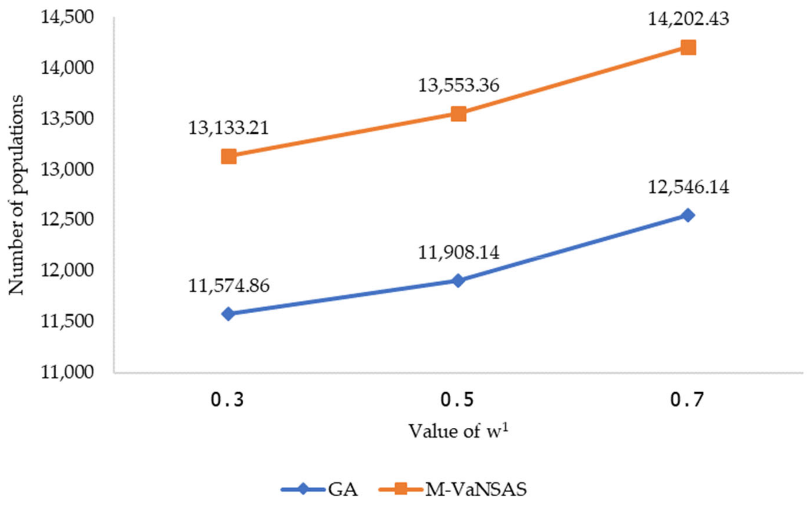
| average | 28,540.43 | 12,546.14 | 27,549.00 | 11,908.14 | 26,862.57 | 11,574.86 | 25,995.43 | 14,202.43 | 25,093.57 | 13,553.36 | 24,457.36 | 13,133.21 |
| %diff | 16.69 | 11.66 | 12.64 | 16.15 | 9.83 | 18.50 | 6.29 | 0.00 | 2.60 | 4.57 | 0.00 | 7.53 |
| Iteration | GA | M-VaNSAS | ||
|---|---|---|---|---|
| Number of Pareto Points | ARP | Number of Pareto Points | ARP | |
| 200 | 280 | 1.4 | 340 | 1.7 |
| 500 | 601 | 1.20 | 891 | 1.78 |
| 800 | 933 | 1.17 | 1023 | 1.28 |
| 1000 | 1284 | 1.28 | 1506 | 1.51 |
| 1200 | 1490 | 1.24 | 1701 | 1.41 |
| 1500 | 1680 | 1.12 | 2014 | 1.34 |
| Average | 1203 | 1.28 | 1362 | 1.46 |
| Best Result from Lingo v.16 | GA | M-VaNSAS | |
|---|---|---|---|
| A-1 | 5.28 | 4.74 | 4.03 |
| A-2 | 5.01 | 4.73 | 4.19 |
| A-3 | 3.45 | 2.93 | 2.04 |
| A-4 | 3.52 | 2.90 | 1.94 |
| A-5 | 3.74 | 2.58 | 1.98 |
| A-6 | 3.02 | 2.30 | 1.74 |
| A-7 | 3.18 | 2.30 | 1.77 |
| A-8 | 3.42 | 2.13 | 1.76 |
| A-9 | 3.45 | 2.13 | 1.69 |
| A-10 | 3.12 | 2.16 | 1.76 |
| A-11 | 4.04 | 2.12 | 1.82 |
| A-12 | 3.56 | 2.05 | 1.86 |
| A-13 | 4.21 | 2.03 | 1.73 |
| A-14 | 4.51 | 2.11 | 1.57 |
| average | 3.82 | 2.66 | 2.13 |
| GA | M-VaNSAS | |
|---|---|---|
| Lingo v.16 | 0.00096 | 0.00096 |
| GA | 0.00096 |
| IB Types | Random-Transit (RT) | Best-Transit (BT) | Inter-Transit (IT) | Scaling Factor (SF) |
|---|---|---|---|---|
| M-VaNSAS-1 | √ | |||
| M-VaNSAS-2 | √ | |||
| M-VaNSAS-3 | √ | |||
| M-VaNSAS-4 | √ | |||
| M-VaNSAS-5 | √ | √ | ||
| M-VaNSAS-6 | √ | √ | ||
| M-VaNSAS-7 | √ | √ | ||
| M-VaNSAS-8 | √ | √ | ||
| M-VaNSAS-9 | √ | √ | √ | |
| M-VaNSAS-10 | √ | √ | √ | |
| M-VaNSAS-11 | √ | √ | √ | |
| M-VaNSAS-12 | √ | √ | √ |
| M-VaNSAS Subalgorithm | |||||||||||||
|---|---|---|---|---|---|---|---|---|---|---|---|---|---|
| Use 1 IB | Use 2 IB | Use 3 IB | Use 4 IB | ||||||||||
| 1 | 2 | 3 | 4 | 5 | 6 | 7 | 8 | 9 | 10 | 11 | 12 | 13 | |
| A-1 | 5.19 | 5.23 | 5.21 | 5.19 | 4.87 | 4.76 | 4.97 | 4.75 | 4.41 | 4.36 | 4.44 | 4.56 | 4.03 |
| A-2 | 5.04 | 5.11 | 5.07 | 5.32 | 4.98 | 4.83 | 4.78 | 4.69 | 4.34 | 4.28 | 4.38 | 4.32 | 4.19 |
| A-3 | 4.45 | 4.58 | 4.62 | 4.37 | 4.13 | 3.89 | 3.84 | 3.89 | 3.52 | 3.14 | 3.26 | 2.87 | 2.04 |
| A-4 | 3.51 | 3.27 | 3.24 | 3.18 | 2.89 | 2.54 | 2.49 | 2.4 | 2.22 | 2.18 | 2.26 | 2.29 | 1.94 |
| A-5 | 3.25 | 3.17 | 3.21 | 3.18 | 2.94 | 2.85 | 2.58 | 2.47 | 2.18 | 1.99 | 2.24 | 2.45 | 1.98 |
| A-6 | 2.78 | 2.92 | 2.65 | 2.59 | 2.43 | 2.57 | 2.49 | 2.28 | 2.11 | 2.08 | 2.42 | 2.31 | 1.74 |
| A-7 | 2.69 | 2.54 | 2.85 | 2.73 | 2.46 | 2.31 | 2.51 | 2.26 | 2.03 | 1.93 | 2.25 | 2.18 | 1.77 |
| A-8 | 2.71 | 2.88 | 2.96 | 2.23 | 2.52 | 2.47 | 2.28 | 2.54 | 2.15 | 2.32 | 2.08 | 2.02 | 1.76 |
| A-9 | 2.65 | 2.71 | 2.59 | 2.64 | 2.28 | 2.32 | 2.39 | 2.31 | 2.18 | 2.26 | 2.29 | 2.18 | 1.69 |
| A-10 | 2.51 | 2.67 | 2.62 | 2.5 | 2.42 | 2.38 | 2.54 | 2.44 | 2.06 | 2.18 | 2.25 | 2.08 | 1.76 |
| A-11 | 2.64 | 2.69 | 2.58 | 2.66 | 2.57 | 2.4 | 2.59 | 2.38 | 2.19 | 2.28 | 2.04 | 2.43 | 1.82 |
| A-12 | 2.78 | 2.5 | 2.63 | 2.73 | 2.64 | 2.66 | 2.71 | 2.73 | 2.26 | 2.31 | 2.18 | 2.37 | 1.86 |
| A-13 | 2.59 | 2.64 | 2.78 | 2.56 | 2.55 | 2.48 | 2.73 | 2.51 | 2.3 | 2.37 | 2.16 | 2.08 | 1.73 |
| A-14 | 2.38 | 2.35 | 2.47 | 2.29 | 2.43 | 2.15 | 2.27 | 2.32 | 1.92 | 1.85 | 2.1 | 1.89 | 1.57 |
| Ave. | 3.23 | 3.23 | 3.25 | 3.16 | 3.01 | 2.90 | 2.94 | 2.86 | 2.56 | 2.54 | 2.60 | 2.57 | 2.13 |
| % dif | 51.64 | 51.64 | 52.58 | 48.36 | 41.31 | 36.15 | 38.03 | 34.27 | 20.19 | 19.25 | 22.07 | 20.66 | 0.00 |
| Average Arrival Time to Patients (min) | Maximum Arrival Time to Patients (min) | Minimum Arrival Time to Patients (min) | Total Cost Incurred (baht) | Total Distance (km) | |
|---|---|---|---|---|---|
| Current situation | 22.48 | 31.72 | 8.10 | 1,718,386 | 8298 |
| GA | 18.60 | 25.01 | 7.05 | 1,348,727 | 6981 |
| M-VaNSAS | 13.37 | 16.95 | 5.04 | 1,167,479 | 5811 |
Publisher’s Note: MDPI stays neutral with regard to jurisdictional claims in published maps and institutional affiliations. |
© 2022 by the authors. Licensee MDPI, Basel, Switzerland. This article is an open access article distributed under the terms and conditions of the Creative Commons Attribution (CC BY) license (https://creativecommons.org/licenses/by/4.0/).
Share and Cite
Sangkaphet, P.; Pitakaso, R.; Sethanan, K.; Nanthasamroeng, N.; Pranet, K.; Khonjun, S.; Srichok, T.; Kaewman, S.; Kaewta, C. A Multiobjective Variable Neighborhood Strategy Adaptive Search to Optimize the Dynamic EMS Location–Allocation Problem. Computation 2022, 10, 103. https://0-doi-org.brum.beds.ac.uk/10.3390/computation10060103
Sangkaphet P, Pitakaso R, Sethanan K, Nanthasamroeng N, Pranet K, Khonjun S, Srichok T, Kaewman S, Kaewta C. A Multiobjective Variable Neighborhood Strategy Adaptive Search to Optimize the Dynamic EMS Location–Allocation Problem. Computation. 2022; 10(6):103. https://0-doi-org.brum.beds.ac.uk/10.3390/computation10060103
Chicago/Turabian StyleSangkaphet, Ponglert, Rapeepan Pitakaso, Kanchana Sethanan, Natthapong Nanthasamroeng, Kiatisak Pranet, Surajet Khonjun, Thanatkij Srichok, Sasitorn Kaewman, and Chutchai Kaewta. 2022. "A Multiobjective Variable Neighborhood Strategy Adaptive Search to Optimize the Dynamic EMS Location–Allocation Problem" Computation 10, no. 6: 103. https://0-doi-org.brum.beds.ac.uk/10.3390/computation10060103