
Optimal Control of a Passive Particle Advected by a Lamb–Oseen (Viscous) Vortex


1
CMUP—Department of Mathematics, FCUP, University of Porto, 4169-007 Porto, Portugal
2
SYSTEC—Department of Electrical and Computer Engineering, FEUP, University of Porto, 4200-465 Porto, Portugal
*
Author to whom correspondence should be addressed.
†
These authors contributed equally to this work.
Computation 2022, 10(6), 87; https://0-doi-org.brum.beds.ac.uk/10.3390/computation10060087
Submission received: 22 April 2022
/
Revised: 13 May 2022
/
Accepted: 25 May 2022
/
Published: 31 May 2022
(This article belongs to the Special Issue Applications of Computational Mathematics to Simulation and Data Analysis)
Abstract
:This work concerns the optimal control of a passive particle in viscous flows. This is relevant since, while there are many studies on optimal control in inviscid flows, there is little to no work in this context for viscous flows, and viscosity cannot always be neglected. Furthermore, in many tasks, there is a need to reduce the energy spent; thus, energy-optimal solutions to problems are important. The aim of this work is to investigate how to optimally move a passive particle advected by a Lamb–Oseen (viscous) vortex between two given points in space in a given time interval while minimising the energy spent on this process. We take a control acting only on the radial component of the motion, and, by using the Pontryagin’s Maximum Principle, we find an explicit time-dependent extremal. We also analyse how the energy cost changes with the viscosity of the flow.The problem is transformed into a parameter search problem with two parameters related to the radial and angular coordinates of the initial point. The energy cost of the process increases with viscosity as long as the passive particle maintains the number of full turns it makes around the vortex. However, the energy cost increases if the increase in viscosity forces the particle to make fewer full revolutions around the vortex.
1. Introduction
In this article, we present a research work developed in the framework of the optimal control of dynamical systems whose state is driven by ordinary differential equations [1,2]. This work provides a solid foundation for the design and control of new, advanced engineering systems, such as (i) underwater gliders, i.e., winged autonomous underwater vehicles (AUVs), moving by modulating their buoyancy, and their attitude in the environment, or (ii) robotic fish. Motion modelling of these two types of systems can be found in [3,4,5], respectively. These systems are useful because they can be used for a variety of automated tasks in a real fluid, such as (i) transporting materials in a flow or (ii) measuring physical quantities of the flow itself, if equipped with the right sensors/tools. Controlling the movement of these robots in a real flow is therefore crucial to be sure that they work as we expect them to.
Vorticity is a useful description of a flow. A vortex is a point with circulation that generates a rotational flow field. Consider a 2D flow specified in the complex plane by N point vortices, each located in [6,7]. In this context, the motion of any passive particle advected by this flow is given by the following dynamical equation
where is the circulation—or strength—of the j-th vortex, and the Cartesian coordinates are specified in a complex formulation as . Table 1 summarises the nomenclature used throughout this article.
However, no flow is completely free of viscosity, and it is important to consider this fact. A simple way to model vortices in a viscous flow is the Lamb–Oseen formulation [8,9], which is the solution of the Navier–Stokes equations for an initial condition in which the full vorticity of the flow is concentrated in a single point in the plane. This originates a vorticity field that decays and is diffused radially outwards with a Gaussian profile (see [6,10]).
An important result about the Lamb–Oseen vortex is that it is an asymptotically stable attracting solution of the vorticity equation for any integrable initial vorticity configuration, as proven by Gallay and Wayne [11]. The superposition of N point vortices is such a configuration, which gave rise to the idea of the multi-Gaussian model. This model assumes that the vorticity field is a superposition of Lamb–Oseen vortices at all times, modelling the behaviour of both the diffusive term and convective term of the vorticity equations through the interaction of the vortices with each other.
More recently, Gallay [12] has shown that under certain conditions, the solution of the Navier–Stokes equations in the inviscid limit for -Dirac initial conditions converges to a superposition of Lamb–Oseen vortices. This provides yet another reason for the suitability of the multi-Gaussian model in the description of fluids.
The motion of a passive particle in such a model should follow the velocity field generated by the system of N vortices, which is given by [13]
where is the kinematic viscosity of the flow. This is consistent with Model (1) as we recover the inviscid equation in the limit .
This work is a continuation of the study made by Marques et al. (2021) [14], where the advection of passive particles is made by an (inviscid) point vortex. In [14], it is shown that the control is explicitly time-dependent, being possible to determine it exclusively by analytical methods. Unfortunately, the same is not possible in the work we are addressing here because of the presence of the viscous terms in Equation (2); therefore, using numerical computation is necessary. In this article, we consider the case for which the dynamic system is driven by one Lamb–Oseen vortex, and we solve a control problem that consists of moving a particle between two given points by applying the necessary conditions of optimality in the form of a maximum principle [15]. We focus on the case where the flow is characterised by a single vortex, and we want to move a single passive particle between two points in the 2D plane by acting only on the radial component of the velocity. The inviscid case () has been studied by Marques et al. (2021) [14]: it is shown that this radial control is explicitly time-dependent and that it can be determined exclusively by analytical methods. Unfortunately, this is not possible in a viscous environment where the dynamical system is driven by a Lamb–Oseen vortex. The viscous terms in the equations of motion (2) hinder the possibility of finding an analytical solution to the problem, so one must resort to numerical computation to find approximate solutions. This article presents a first study of this problem in a viscous environment: we consider the case where the dynamical system is driven by a single Lamb–Oseen vortex, and we solve a control problem consisting of moving a particle between two given points by applying necessary optimality conditions in the form of a maximum principle [15]. This problem follows the idea of the more general Problem 2 proposed in Protas [16]. Section 2 and Section 3 are devoted to the mathematical formulation of the problem. In Section 4, we derive the optimal control and study the optimal trajectories for the passive particle for different kinematic viscosities. The conclusions and future work constitute the last section.
2. Velocity Field Driven by a Lamb–Oseen Vortex
Consider a viscous flow with some kinematic viscosity and a Lamb–Oseen vortex at the origin , with vorticity k. Let be the position of a passive particle placed in this flow at time t. In the complex formulation, the dynamic equation for the particle positioned in z subject to the velocity field generated by the vortex is
In polar coordinates, the position of the particle is given by
and the derivative with respect to t is
By separating the equalities of the real and imaginary parts of both sides of the equation, we have the following dynamic equations for the particle in polar form
which are not solvable analytically. However, it is easy to qualitatively characterise the motion of the particle: it is a circular motion with a constant radius and a variable angular velocity that decreases to 0 as time approaches ∞.
3. Control Problem
Consider a flow like the one presented in Section 2 and a passive particle placed in the flow with initial position . The objective of this problem is to determine the control function to be applied to the particle so that it moves in the flow from the given initial position to the endpoint while minimising the cost function while subject to the flow field. Let be the position of the particle at time t. The control problem can be formulated as follows:
The maximum principle [15] allows us to determine the set of optimal control candidates by using the maximisation of the Pontryagin–Hamiltonian function (here, P is the adjoint variable satisfying along the optimal reference control process, where is the gradient of H with respect to X) almost everywhere with respect to the Lebesgue measure (from here on, functions are specified in this sense), together with the satisfaction of the appropriate boundary conditions.
4. Minimum Energy Problem
Our cost function here is the total control power consumption, i.e., the energy used to move the particle,
We want to minimise the power spent to move the particle between some specified initial and final points so that the particle is at at the final time T.
To obtain the Mayer’s problem, we consider a new variable satisfying the condition . Our control problem can thus be formulated as follows:
In addition, we impose the radial velocity approaches zero at so that the control is smooth and differentiable during the arrival at the circular trajectory of radius . For simplicity, we will only consider the case where . The case follows analogously.
For this problem, the Pontryagin–Hamiltonian function is
and the dynamic equations for the adjoint variable are
While the differential equation for is impossible to solve analytically, from the transversality conditions, it is possible to further conclude that and that is constant ().
Thus, the Pontryagin–Hamiltonian function can be rewritten as
Furthermore, we know that the optimal control should maximise the Hamiltonian at any time; thus,
and the optimal control should satisfy
While the angular motion of the particle follows the same dynamic equation independently of the control, it is possible to distinguish between two different behaviours for the radial motion of the passive particle:
(a) If ,
(b) If , then we have
If at a certain point of the process, it means that the time T is not sufficient to complete the transport of the particle without applying the control . This constant control is more energy-consuming than a variable control implicitly defined by the nonlinear Equation (17). In this scenario, we start by applying the control for the time period until the particle is in a state where it can be brought to the final position by applying the variable control in the remaining time .
Unfortunately, there is no way to explicitly calculate to determine the switching points for the control. Therefore, to solve the problem, we have to take a different approach. We now analyse the case where throughout the whole process.
If the trajectory never uses the control , then we can divide the motion of the passive particle into two regimes. During the first regime of motion, the particle is pulled radially inwards by a variable control from until its radial coordinate reaches at an unspecified time . The angular motion is influenced by two different factors: the fact that the particle approaches the vortex contributes to the acceleration of the motion, while the fact that the vortex loses strength over time due to the viscosity of the fluid contributes to the deceleration of the motion.
The movement of the particle during this regime is determined by the solution of the following differential equations, valid for the time interval :
Notice that for and that we cannot solve this problem because we do not know a priori the value of . However, assuming we could, the particle would end at the point in polar coordinates.
The second regime of the motion happens when the particle is describing a circular motion of constant radius in the time interval and follows the differential equations
In order to solve this problem, we have to work backwards from the final point since this second regime of motion has an actual (numerically) solvable system of differential equations. Note, however, that solving this control problem is now reduced to finding for the parameters and that give us a solution of Systems (18) and (19) with minimal energy. We first investigate how the solutions of these systems behave when we change these parameters.
In each of the following studies, the approximate solutions of the differential equations were obtained through the Runge–Kutta–Fehlberg method [17] with a step size of s. All results presented below use SI units. Viscosity values depend on the physical conditions of the fluid such as temperature and are typically in the range of – ms. For example, typical seawater at 20 °C has a low kinematic viscosity of about ms, while typical printer inks at about 38 °C can have viscosities of up to ms.
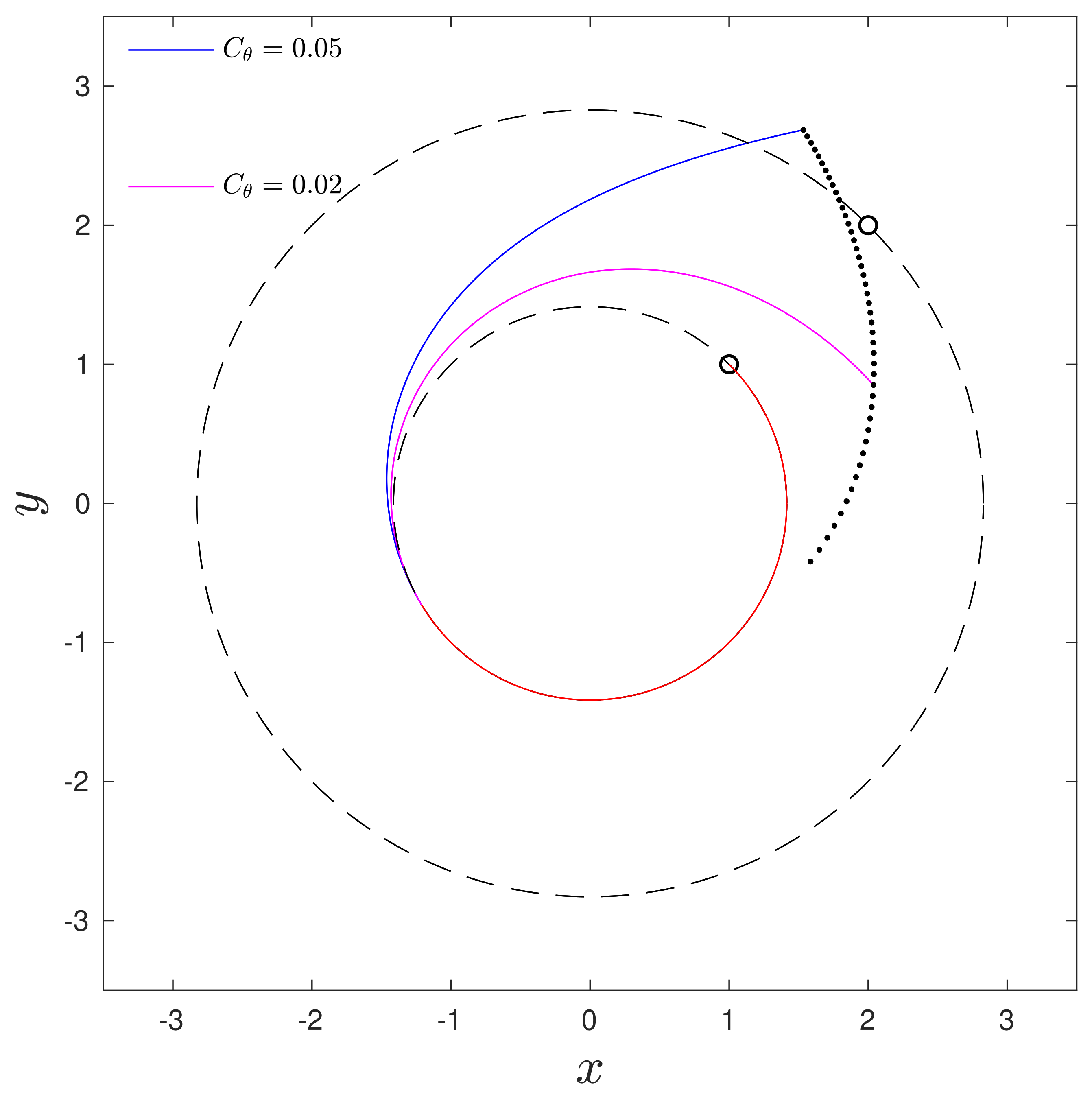
In order to check how the parameters affect the solutions of this problem, we set ms, m, m, , ms and s. In Figure 1, we set s and varied . The large dashed circumferences correspond to circular trajectories of radius m and m, the open circles identify the specified initial and final points for the problem, and the red curve represents the trajectory of the particle corresponding to the second regime of motion. The blue and pink lines represent two possible trajectories for the particle in the first regime of motion, corresponding to different values for . The black dots correspond to a variety of possible initial positions for the simulation, each for a different . We note that the radial coordinate of the initial position increases with and that changing this parameter alone is not sufficient to retrieve the desired initial position. Therefore, must play a role in this.
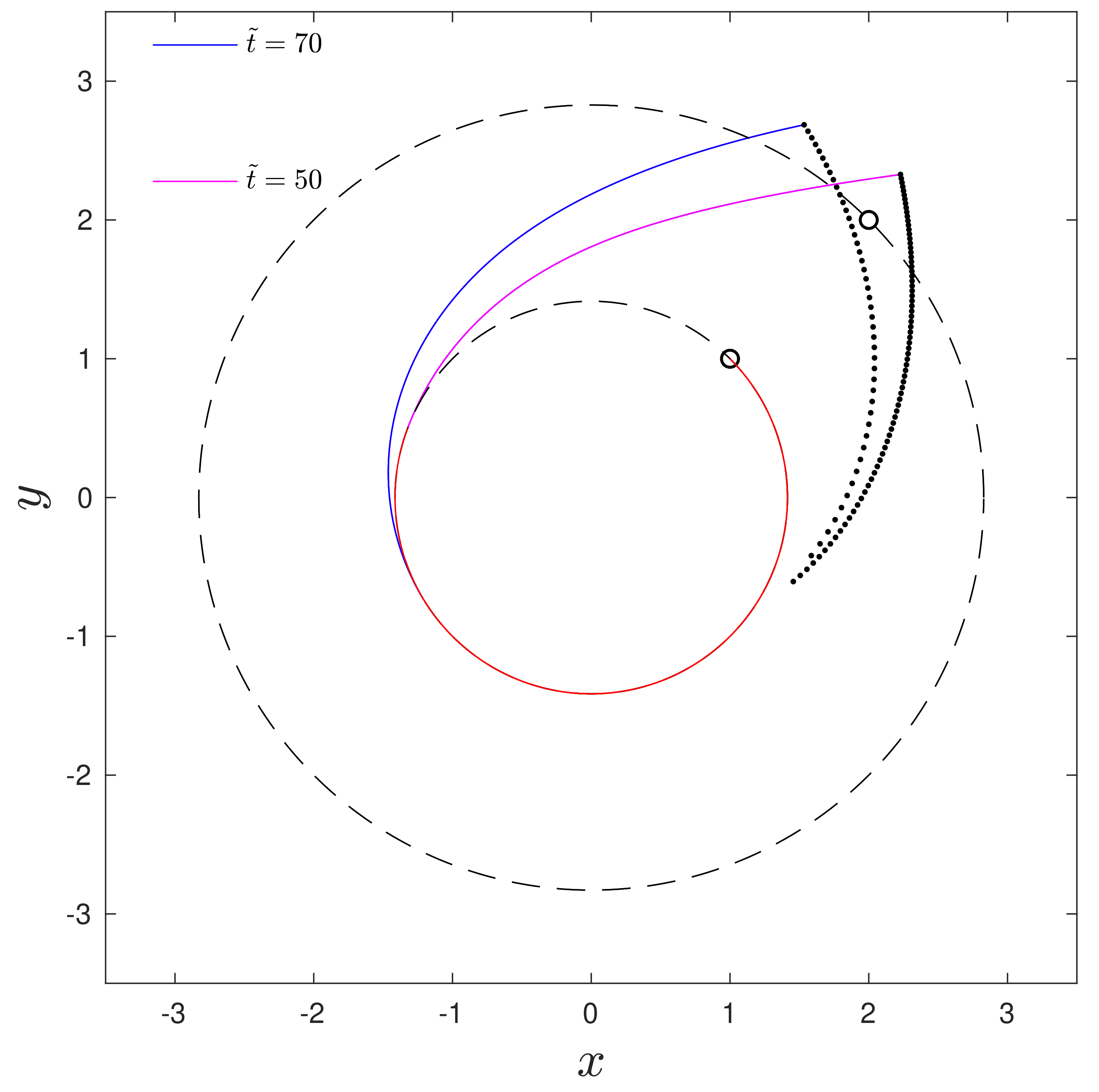
Figure 2 is similar to Figure 1 but now illustrates how the initial position for the simulations is affected by the parameter . We see that for a radial coordinate equal to that of the initial position of the particle, larger values of will result in simulated initial points with a larger angular coordinate. Thus, we can think of as the parameter that controls the radial coordinate and as the parameter that controls the angular coordinate for the simulated initial position.
From this behaviour, it is possible to develop a simple algorithm to solve the proposed control problem. The idea is as follows: From this behaviour, we develop a simple algorithm to solve the proposed control problem. The idea is as follows:
- (1)
- Arbitrate a . Find two distinct values , which give rise to two curves of simulated initial positions that go under and over the initial position (like the dotted curves in Figure 2);
- (2)
- Solve Equation (19) backwards in time from T to = in order to obtain ;
- (3)
- Arbitrate a . Find an interval of values for such that if and if ;
- (4)
- (5)
- After attaining , check for : if , adjust to a lower value; if , adjust to a higher value; if , adjust ; if , adjust . Repeat the process from (2) until .
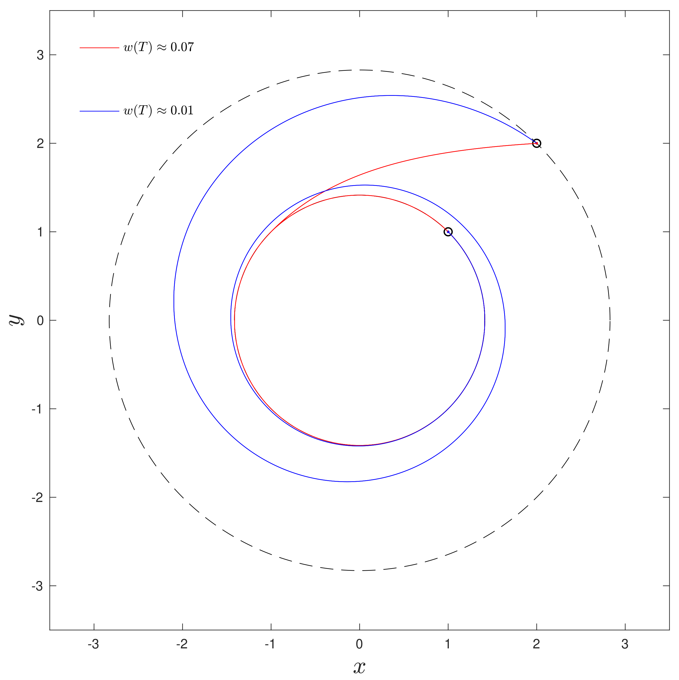
Using this technique, we can analyse the possible candidates for the optimal solutions to the problem and identify the one that minimises the energy spent on moving the particle. For example, Figure 3 shows two possible solutions to the problem with ms, m, m, , ms and s. These two solutions are candidates that arose from the maximum principle, yet the solution shown in red has a higher energy cost than the one depicted in blue. The existence of multiple candidates arises in the case where T is large enough to allow the particle to circle around the vortex multiple times. The optimal solution is the one in which the particle makes the fewest revolutions on the trajectory of a smaller radius, i.e., the solution in which the control is active for the most time. This is due to the quadratic cost function: it is better to pull the particle slowly inwards over a longer period of time than to pull it quickly over a shorter period of time.
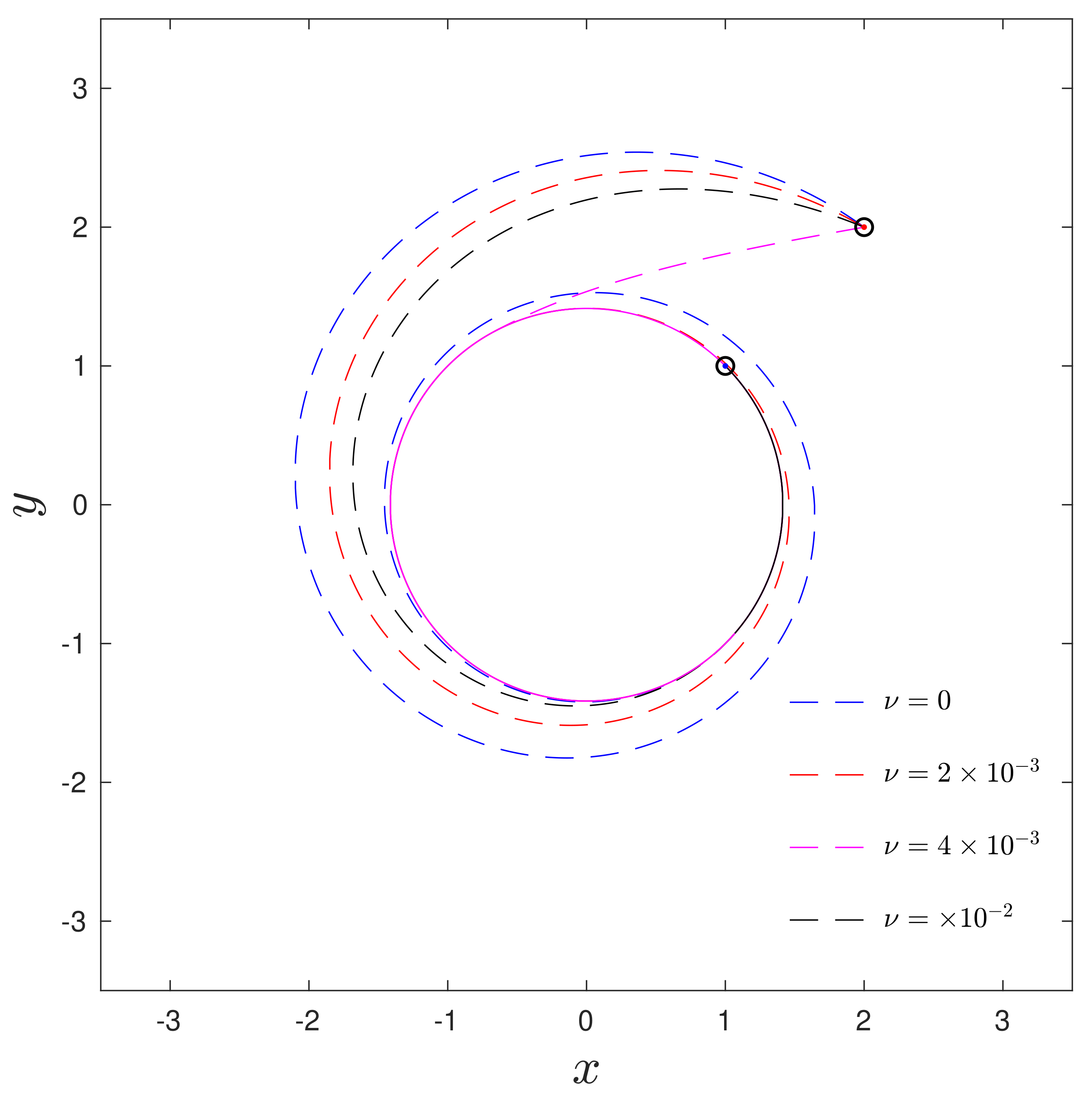
Finally, we investigate the behaviour of solutions when we change the viscosity of the environment. We worked once again on the problem with m, m, , ms and s. In Table 2, we summarise the parameters and that we found for the optimal solution for different kinematic viscosities ranging from ms to ms, as well as the energy costs in each of these scenarios. For completeness, the analytical values for ms are also given (from Marques et al. [14]). Note that for low viscosity, the rounded values might be the same, but they actually differ in decimal places, which are not shown and can be computed to any desired accuracy as long as it is within the machine’s reach.
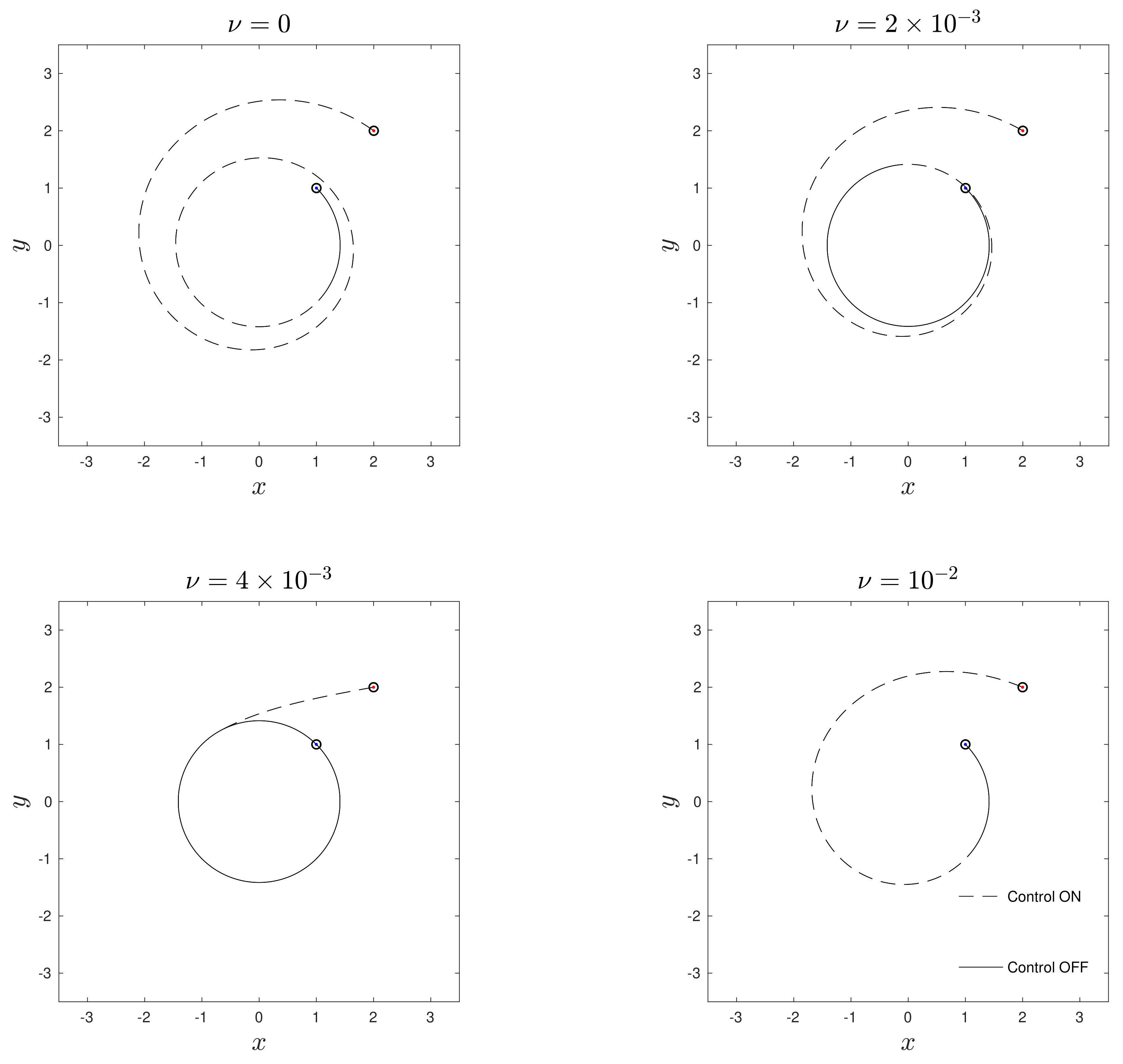
As expected, the energy cost seems to increase with viscosity, as we have to put more force into the system to move the particle through a more viscous flow. However, there are jumps in this behaviour as we can see when comparing the scenarios of ms, ms and ms (for a visual representation of these optimal trajectories, see Figure 4 and Figure 5). The increase in viscosity changes the possible trajectories for the particle in their nature. In the case where ms, the parameters allow for two types of solutions: one where the particle makes less than one complete turn around the vortex under the control (and then more than one full revolution around the vortex under no control) and a second where the particle makes more than one complete turn around the vortex under the control (and then less than a complete revolution around the vortex under no control). This is the same scenario as in Figure 3, and the optimal trajectory that minimises the energy cost is the one where the control is active for the longest time. Increasing the viscosity to ms is sufficient to exclude this second type of trajectory from the possible optimal trajectories, and we are left with the sole possibility of a trajectory where the particle is pushed harder and faster into a circular trajectory with the same radius as the final point and then makes more than one full revolution around the vortex while subject only to the velocity field of the flow. This increases the energy cost considerably. If we increase the viscosity further—to ms—we are now in a scenario where the particle cannot reach the target point in two complete turns around the vortex, and the optimal trajectory requires only one complete revolution around the vortex. The fact that we now need one less revolution around the vortex to move the particle significantly reduces the energy cost of the process.
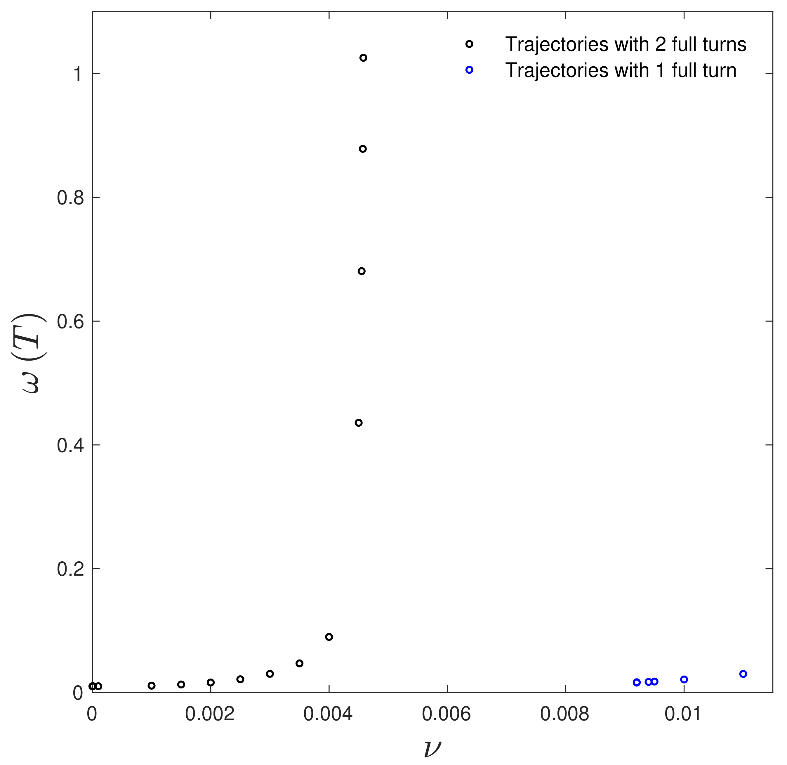
Thus, in fact, the energy cost of displacing a particle in this scenario increases with viscosity as long as the number of revolutions required to reach the final remains the same. If the number of turns needed to complete the process decreases, the energy cost of the displacement decreases. This is illustrated in Figure 6, where we plot the viscosity of the flow against the energy cost for the optimal solution.
The region where the number of revolutions of optimal solutions changes is difficult to analyse, as we have no way of finding the optimal solution in the scenario where there is a time frame where the control is active. These types of solutions lie in this region. It is also not known whether it is possible to find a solution for any value of kinematic viscosity for a given problem. This is particularly difficult to analyse around the switching point of the number of revolutions of optimal solutions.
5. Conclusions and Future Work
The full Navier–Stokes equations are difficult to analyse and integrate. The task becomes even more hazardous if we want to combine the full description of flows with optimal control. The point vortex description of flows preserves the more important nonlinear features of the full flow description and, being a low-dimensional description, allows us to deal with more complex problems, such as the optimal control of flows. Although there has been some work on optimal control of inviscid vortices, the literature on the optimal control in viscous vortex flows is still scarce. We study how to optimally move a passive particle between two points in space in a given time in a viscous flow where the dynamics are driven by a Lamb–Oseen vortex. Even though the case study presented here is simple, it cannot be solved explicitly due to the nature of the differential equations arising from the maximum principle. However, it is possible to understand how the solutions behave and transform the problem into a parameter-search problem. We analyse how these parameters affect the optimal trajectories of a passive particle in a viscous environment ruled by a Lamb–Oseen vortex and how the energy cost is affected by the viscosity of the flow. In order to solve it, we turn the problem around and look for a way to move the particle from the final position to the initial position. Two parameters appear in the equations: , which affects the radial coordinate of the initial position, and , which affects the angular coordinate of the initial position. Furthermore, we find that the energy cost of displacing a particle in such a scenario (i) increases with viscosity as long as the number of complete revolutions around the vortex remains the same; (ii) decreases when the viscosity increases such that that the number of complete turns required for the process decreases. We plan to conduct further research in this area, in particular analysing the behaviour of solutions where the control is active during a certain period of time and eventually tackling an environment with multiple vortices or using different types of admissible controls.
Author Contributions
Conceptualization, G.M., S.G. and F.L.P.; methodology, G.M., S.G. and F.L.P.; software, G.M.; validation, G.M.; formal analysis, G.M., S.G. and F.L.P.; investigation, G.M., S.G. and F.L.P.; writing—original draft preparation, G.M.; writing—review and editing, G.M.; supervision, S.G. and F.L.P.; funding acquisition, G.M., S.G. and F.L.P. All authors have read and agreed to the published version of the manuscript.
Funding
This work was partially supported by (i) grant ref. PD/BD/150537/2019 through Fundação para a Ciência e a Tecnologia (FCT); (ii) CMUP, ref. UIDB/00144/2020 funded through FCT; (iii) SYSTEC, ref. POCI-01-0145-FEDER-006933 funded by ERDF | COMPETE2020 | FCT/MEC | PT2020; (iv) project MAGIC POCI-01-0145-FEDER-032485, funded by FEDER via COMPETE 2020—POCI and by FCT/MCTES via PIDDAC; and (v) project SNAP NORTE-01-0145-FEDER-000085, funded by the European Regional Development Fund (ERDF), through the North Portugal Regional Operational Programme (NORTE2020), under the PORTUGAL 2020 Partnership Agreement.
Institutional Review Board Statement
Not applicable.
Informed Consent Statement
Not applicable.
Data Availability Statement
Not applicable.
Conflicts of Interest
The authors declare no conflict of interest.
References
- Clarke, F.; Ledyaev, Y.; Stern, R.; Wolenski, P. Nonsmooth Analysis and Control Theory; Springer: New York, NY, USA, 1998. [Google Scholar]
- Lions, J. Optimal Control Of Systems Governed by Partial Differential Equations; Springer: New York, NY, USA, 1971. [Google Scholar]
- Mahmoudian, N.; Geisbert, J.; Woolsey, C. Dynamics and Control of Underwater Gliders I: Steady Motions; Technical Report; Virginia Center for Autonomous Systems: Blacksburg, VA, USA, 2009. [Google Scholar]
- Mahmoudian, N.; Woolsey, C. Dynamics and Control of Underwater Gliders II: Motion Planning and Control; Technical Report; Virginia Center for Autonomous Systems: Blacksburg, VA, USA, 2010. [Google Scholar]
- Liu, J.; Hu, H. Biological Inspiration: From Carangiform Fish to Multijoint Robotic Fish. J. Bionic Eng. 2010, 7, 35–48. [Google Scholar] [CrossRef]
- Batchelor, G.K. An Introduction to Fluid Dynamics; Cambridge University Press: New York, NY, USA, 1992. [Google Scholar]
- Newton, P.K. The N-Vortex Problem—Analytical Techniques; Springer: New York, NY, USA, 2001. [Google Scholar]
- Oseen, C.W. Uber die Wirbelbewegung in einer reibenden Flussigkeit. Ark. Mat. Astro. Fys. 1912, 7, 14–26. [Google Scholar]
- Saffman, P.G.; Ablowitz, M.J.; Hinch, J.E.; Ockendon, J.R.; Olver, P.J. Vortex Dynamics; Cambridge University Press: Cambridge, UK, 1992. [Google Scholar]
- Pope, S.B. Turbulent Flows; Cambridge University Press: Cambridge, UK, 2000. [Google Scholar]
- Gallay, T.; Wayne, C.E. Global Stability of Vortex Solutions of the Two-Dimensional Navier-Stokes Equation. Commun. Math. Phys. 2005, 255, 97–129. [Google Scholar] [CrossRef] [Green Version]
- Gallay, T. Interaction of Vortices in Weakly Viscous Planar Flows. Arch. Ration. Mech. Anal. 2011, 200, 445–490. [Google Scholar] [CrossRef] [Green Version]
- Kim, S.-C.; Sohn, S.I. Interactions of Three Viscous Point Vortices. J. Phys. A Math. Theor. 2012, 45, 455501. [Google Scholar] [CrossRef]
- Marques, G.; Grilo, T.; Gama, S.; Pereira, F.L. Optimal Control of a Passive Particle Advected by a Point Vortex. In Advanced Research in Technologies, Information, Innovation and Sustainability; Springer: Cham, Switzerland, 2021; pp. 512–523. [Google Scholar]
- Pontryagin, L.; Boltyanskiy, V.; Gamkrelidze, R.; Mishchenko, E. Mathematical Theory of Optimal Processes; Interscience Publish: New York, NY, USA, 1962. [Google Scholar]
- Protas, B. Vortex dynamics models in flow control problems. Nonlinearity 2008, 21, 203–250. [Google Scholar] [CrossRef]
- Fehlberg, E. Low-Order Classical Runge-Kutta Formulas with Stepsize Control and Their Application to Some Heat Transfer Problems; Technical Report 315; NASA: Washington, DC, USA, 1969. [Google Scholar]
Figure 1.
We want to move the particle from to . The red line represents the motion of the particle during the second regime, while the blue and pink lines represent two possible trajectories on the first regime for different . The black dots represent possible initial positions for the particle for different values of . We see that even if we change , we cannot reach the desired initial position (represented by the open circle), so we have to change .

Figure 2.
We want to move the particle from to . The red line represents the motion of the particle in the second regime, while the blue and pink lines represent two possible trajectories in the first regime for different and . The black dots represent possible initial positions for the particle for different values of these parameters. We see that a change in affects the radial coordinate, while a change in affects the angular coordinate of the simulated initial point.

Figure 3.
Depiction of two possible solutions for the problem with parameters ms, m, m, , ms and s. The solution depicted by the blue line is optimal since it has a lower energy cost () than the one depicted in red (). Both of these candidates arose from applying the maximum principle to the problem.

Figure 4.
Optimal trajectories for the particle in the problem with parameters m, m, , ms and different kinematic viscosities for the flow. The dashed lines correspond to the part of the trajectory where the control is active, and the solid lines indicate the part of the trajectory where the control is off. For comparison, the scenario ms is shown, and the trajectory is drawn with the parameters obtained analytically from the expressions given by Marques et al. [14].

Figure 5.
Optimal trajectories for the particle in the problem with parameters m, m, , ms and different kinematic viscosities for the flow. The dashed lines correspond to the part of the trajectory where the control is active, and the solid lines indicate the part of the trajectory where the control is off. For comparison, the scenario ms is shown, and the trajectory is drawn with the parameters obtained analytically from the expressions given by Marques et al. [14].

Figure 6.
Energy cost for the problem with parameters m, m, , ms and different kinematic viscosities for the flow. The cost increases with viscosity for solutions of the same nature (i.e., the number of full turns of the particle around the vortex), but there is a sharp decrease in energy when the nature of the solution changes to a smaller number of complete revolutions.


Table 1.
Nomenclature table.
| Symbol | Meaning | SI Units |
|---|---|---|
| t | Time | s |
| Position in polar coordinates | m | |
| Radial coordinate | m | |
| Angular coordinate | rad | |
| k | Circulation | ms |
| Kinematic viscosity | ms | |
| u | Control | ms |
Table 2.
Values of the parameters and energy costs for the optimal solutions of the problem with m, m, , ms and s for various kinematic viscosities. The scenario is presented for comparison, and the values of the parameters were calculated analytically from Marques et al. [14].
Table 2.
Values of the parameters and energy costs for the optimal solutions of the problem with m, m, , ms and s for various kinematic viscosities. The scenario is presented for comparison, and the values of the parameters were calculated analytically from Marques et al. [14].
| (m) | 0 | ||||||
|---|---|---|---|---|---|---|---|
| (s) | 232.89 | 232.87 | 232.87 | 220.97 | 156.20 | 26.49 | 163.32 |
| (ms) | 0.0014 | 0.0014 | 0.0014 | 0.0018 | 0.0043 | 0.11 | 0.019 |
| w (T) | 0.010 | 0.010 | 0.010 | 0.011 | 0.016 | 0.090 | 0.021 |
Publisher’s Note: MDPI stays neutral with regard to jurisdictional claims in published maps and institutional affiliations. |
© 2022 by the authors. Licensee MDPI, Basel, Switzerland. This article is an open access article distributed under the terms and conditions of the Creative Commons Attribution (CC BY) license (https://creativecommons.org/licenses/by/4.0/).
Share and Cite
MDPI and ACS Style
Marques, G.; Gama, S.; Pereira, F.L. Optimal Control of a Passive Particle Advected by a Lamb–Oseen (Viscous) Vortex. Computation 2022, 10, 87. https://0-doi-org.brum.beds.ac.uk/10.3390/computation10060087
AMA Style
Marques G, Gama S, Pereira FL. Optimal Control of a Passive Particle Advected by a Lamb–Oseen (Viscous) Vortex. Computation. 2022; 10(6):87. https://0-doi-org.brum.beds.ac.uk/10.3390/computation10060087
Chicago/Turabian StyleMarques, Gil, Sílvio Gama, and Fernando Lobo Pereira. 2022. "Optimal Control of a Passive Particle Advected by a Lamb–Oseen (Viscous) Vortex" Computation 10, no. 6: 87. https://0-doi-org.brum.beds.ac.uk/10.3390/computation10060087
Note that from the first issue of 2016, this journal uses article numbers instead of page numbers. See further details here.