Investigation of Statistical Machine Learning Models for COVID-19 Epidemic Process Simulation: Random Forest, K-Nearest Neighbors, Gradient Boosting

Abstract

COVID-19 has become the largest pandemic in recent history to sweep the world. This study is devoted to developing and investigating three models of the COVID-19 epidemic process based on statistical machine learning and the evaluation of the results of their forecasting. The models developed are based on Random Forest, K-Nearest Neighbors, and Gradient Boosting methods. The models were studied for the adequacy and accuracy of predictive incidence for 3, 7, 10, 14, 21, and 30 days. The study used data on new cases of COVID-19 in Germany, Japan, South Korea, and Ukraine. These countries are selected because they have different dynamics of the COVID-19 epidemic process, and their governments have applied various control measures to contain the pandemic. The simulation results showed sufficient accuracy for practical use in the K-Nearest Neighbors and Gradient Boosting models. Public health agencies can use the models and their predictions to address various pandemic containment challenges. Such challenges are investigated depending on the duration of the constructed forecast.

1. Introduction

The COVID-19 virus was first reported in December 2019 [1]. Chinese authorities told the World Health Organization (WHO) that a man died from a respiratory disease of unknown origin in Wuhan, Hubei province. In early January 2020, it was revealed that the genome of a new type of coronavirus is similar to the genome of the SARS virus that spread worldwide from China in 2002–2003 [2]. Initially, the new coronavirus was treated by the world health system as an epidemic of a regional scale, affecting only China. Nevertheless, in the first month, the virus began to spread rapidly outside of China and threatened the health of the entire planet’s population [3]. On 11 March 2020, the WHO declared a global pandemic of COVID-19.

The entire world community has directed efforts to prevent and combat the new coronavirus. The virus has spread across the globe through tourists and the availability of flights. In the spring of 2020, restrictive measures were introduced in most countries to contain the spread of COVID-19 [4]. Among such activities were lockdowns, contact tracing with isolation of contact individuals, the introduction of a mask regime, social distancing, etc. As the epidemic was contained, the authorities of individual countries began to gradually ease lockdowns and other restrictive measures to minimize damage to the economy and prevent social problems [5]. In the fall of 2020, the second and third waves of the epidemic began in many countries [6]. New strains of the virus began to spread, characterized by increased virulence [7].

A large-scale vaccination campaign, which was launched in a short time around the world, contributed significantly to the fight against COVID-19 [8]. The development of vaccines against coronavirus diseases, such as SARS and MERS, which began even before the onset of the COVID-19 pandemic, made it possible to form knowledge about the structure and rules of the coronaviruses spread [9]. Furthermore, it is this knowledge that has accelerated the development of various types of vaccines during the current pandemic. Many countries have introduced phased population vaccination plans, identifying groups at the highest risk of complications. Inactivated vaccines, live attenuated vaccines, vector non-replicating and vector replicating vaccines, vector inactivated, DNA and RNA vaccines, and recombinant protein vaccines have been developed. Some of them were used to combat the pandemic.

The unprecedented crisis caused by the global COVID-19 pandemic has demonstrated the significant role of digital technologies [10]. Since the beginning of the pandemic, the world has seen an accelerated digitalization of many activities, such as the economy [11], finance [12], business [13], transport [14], education [15], and many others. Digitalization has not bypassed the field of medicine with the improvement of diagnostic methods [16], automated processing of medical data [17], and storage of medical data [18]. Models and methods for modeling epidemic morbidity received a new round.

This study aims to develop three models for predicting the dynamics of the COVID-19 epidemic process in specific areas using statistical machine learning methods and to study the results of the experiments of the constructed models.

To achieve this goal, the following tasks were formulated:

• To analyze models and methods for modeling the epidemic process of COVID-19.
• To analyze data on the incidence of COVID-19 in the selected territories.
• To develop a model for predicting the dynamics of the COVID-19 epidemic process based on the K-Nearest Neighbors method.
• To develop a model for predicting the dynamics of the COVID-19 epidemic process based on Gradient Boosting.
• To develop a model for predicting the dynamics of the COVID-19 epidemic process based on the Random Forest method.
• To evaluate the results of an experimental study using the developed models.
• To analyze the developed models for accuracy and computational complexity.

The promising contribution of this study is two-stage. First, the development of models based on statistical machine learning methods will make it possible to assess the accuracy of forecasts of the dynamics of the COVID-19 epidemic process built using simple models. Secondly, a comparative study of three models of statistical machine learning will allow us to conclude which of them is more effective for studying the epidemic processes not only of COVID-19 but also of other infectious diseases.

The further structure of the paper is the following: Section 2, Current Research Analysis, provides an overview of models and methods of epidemic process simulation. Section 3, Data on COVID-19 Morbidity Analysis, provides a brief description of the COVID-19 pandemic in countries investigated within the research: Germany, Japan, South Korea, and Ukraine. Section 4, Model and Methods, describes three regression approaches to COVID-19 morbidity forecasting. Section 4, Results, describes the results of models’ performance, estimation of developed models’ adequacy, and forecasting accuracy. Section 5, Discussion, discusses the perspective use of models and their limitations. The conclusion describes the outcomes of the research.

Research is part of a complex intelligent information system for epidemiological diagnostics, the concept of which is discussed in [19].

2. Current Research Analysis

The field of modeling epidemic processes originated at the beginning of the 20th century with the works of Ronald Ross [20], William Hamer [21], Anderson McKendrick, and William Kermack [22]. The works of these scientists laid the mathematical foundations of epidemiology, proposing to describe the dynamics of morbidity using compartmental models [23]. In such models, the population is divided into compartments depending on their belonging to a defined state. The epidemic process occurring in the population is described using systems of differential equations.

Compartment models are used to model and study many infectious diseases. The paper [24] describes the application of compartmental models to study measles incidence. Double vaccination was considered, and the model was studied for balance and stability. The results show that the rate of transmission of infection has the most significant impact on the incidence of measles. In [25], the incidence of influenza was considered, and the classical SIR model was studied. The application of the probabilistic approach in the transition between states is considered. It is concluded that the negative aspect of applying the compartmental approach to modeling influenza is the non-obviousness of the results concerning one or even several scenarios of the development of the epidemic. The compartmental approach to influenza modeling was used as early as the 1970s by Baroyan and Rvachev [26]. The simulation results were used in the USSR to substantiate anti-epidemic measures aimed at combating the increase in the incidence of influenza.

Among intestinal infections, a compartmental approach is applied to modeling salmonellosis. The study [27] considered non-infectious and endemic resistant states. The model itself is not accurate enough to conduct relevant experiments to study the dynamics of Salmonella bacterial infection. The model of the hepatitis A built-in [28] aims to assess the impact of various vaccination strategies. The results show the importance of hepatitis A vaccination in early childhood.

In [29], an air-borne infection diphtheria incidence model was constructed by extending the classical SIR model. The authors found a globally asymptotically stable equilibrium of infectious extinction. However, such results cannot be effectively interpreted in epidemiology and public health.

The compartmental approach also applies to infections with a contact route of transmission. The work [30] is devoted to modeling HIV/AIDS with the possibility of treatment. The authors have proved that painless equilibrium is globally asymptotically stable when the base reproduction number is less than one. However, such a conclusion is a law of epidemiology and does not require analytical proof using modeling tools. The model of hepatitis B described in [31] shows the importance of assessing population migration for the spread of the disease. The authors claim that it is possible to reduce the incidence of hepatitis B based on the model results. However, the main vectors of the infection are not taken into account when compiling compartments. The authors of [32] describe a model of the epidemic process of hepatitis C. The emphasis is on people who inject drugs. The model is dynamic and interactively presented using a web application. The disadvantage of the model is that if there is a significant change in the rules of distribution, for example, the introduction of a policy to combat injecting drug users or the introduction of mass substitution therapy, all model parameters must be adjusted again.

A common disadvantage of the models described above is the impossibility of extending them to other objects. It is necessary to completely rebuild the model and find new coefficients related to a particular disease to model another disease.

With the onset of the global COVID-19 pandemic, compartmental models are actively used to model the epidemic process of a new coronavirus in various territories. Such territories can have different sizes, densities, and populations. Thus, in [33], the territory of the college campus is considered, where complex public health protocols can be introduced. In [34], the spread of COVID-19 in New York is modeled to determine the peak of the incidence wave. The work [35] extends the territory of modeling to the state of New York. It examines strategies to manage the course of the epidemic based on control measures implemented in other states. In [36,37], the dynamics of COVID-19 are modeled on the island states, limited from the outside world of Sri Lanka and Cyprus. In the case of Sri Lanka, the emphasis is on the isolation of villages on the island and the absence of tourists. When modeling the epidemic situation in Cyprus, an arbitrary number of subgroups with different infection levels and testing were used. In [38], an entire country was taken to model COVID-19: France. New cases, deaths, hospitalizations, intensive care unit admissions, hospital deaths, etc., are used. In [39], several European countries are considered at once, and for each country, its transmission coefficients, recovery rates, etc., are calculated. Considering compartmental models for different areas, it should be noted that even when studying a single disease, such as COVID-19, the coefficients of the model should be found again for each area, and the system of differential equations should be rebuilt from the very beginning.

Compartmental approaches with different sets of states are also used to model COVID-19. The study [40] uses the simplest SIR (susceptible—infected—recovered) model. The disadvantage of the model is the accuracy of forecasts, which is insufficient for decision-making, and the limitedness in population groups gives a very general understanding of the spread of the epidemic process. In [41], the classical SIR model is extended by adding the exposed state. The model is used to find the peak of the disease, but the results have not materialized due to changes in the policy of control measures in the countries considered and the start of the vaccine campaign. The work [42] extends the classical SIR model with the state Q—quarantined for isolated infected people. The model shows that the maximum number of infected in the real world is highly dependent on the speed with which quarantine restrictions are implemented. The authors of [43] add the D-death state to the SEIR model for fatal cases. Modeling results show that unreported deaths from COVID-19 are significantly lower than unreported infections. In [44], the authors extend the SEIR model with the state Q—quarantined. At the same time, the model does not consider isolation scenarios and social distancing. The study [45] extends the SEIR model with states D—death and Q—quarantined. Moreover, the quarantined state means hospitalization since the authors hypothesize that hospitalization is similar to quarantine restrictions. In this case, the model considers the average behavior of the population, which leads to an underestimation of specific population groups. In [46], the authors present a model consisting of seven compartments: susceptible (S), exposed (E), infectious (I), quarantined (Q), recovered (R), deaths (D), and vaccinated (V). The model can estimate predicted numbers of compartments, but only for a short time. Models with a much larger number of compartments are also known. However, a common disadvantage is that many states and subpopulations are needed to adequately describe a population, which makes models complex. The complexity of the models causes both difficulties with calculations and experimental studies and the impossibility of promptly making changes to the model when the behavior of the virus dynamics changes.

Models are also used for various tasks in the study of COVID-19. For example, work [47] considers the effectiveness of vaccination distribution. The study [48] looks at the transport effects of the COVID-19 pandemic. In [49], the effectiveness of the introduction of lockdowns is estimated. Ref. [50] explores the effects of social distancing. The authors of [51] investigate the effectiveness of masks to combat the novel coronavirus pandemic. The study [52] is devoted to assessing the economic aspects of applying control measures to combat the COVID-19 pandemic. Work [53] uses compartmental models to investigate the transmission of the COVID-19 virus among medical personnel and methods for protecting healthcare workers from infection. Ref. [54] uses modeling to estimate the medical throughput of hospitalization, including for intensive care units.

However, the compartmental approach to modeling infectious diseases, including COVID-19, has several disadvantages, among which are the following:

• An accurate description of the population in which the epidemic process spreads requires considering the population’s heterogeneity, i.e., age, gender, behavior, physical interaction, etc. However, introducing all these characteristics into the compartmental model significantly complicates it and makes it unsuitable for practical use.
• The apparatus of differential equations has high computational complexity with sufficiently detailed models.
• Different diseases have different conditions and rules of infection transmission in different population groups, making it impossible to transfer an already ready model for one infectious disease to another disease. So, for each new disease, the model must be rebuilt.
• The same model cannot be applied in different territories even for the same disease because transfer rules and control measures may differ depending on the location, climate, legal aspects, etc. For each new territory, the model needs to be built anew.
• When the virulence of the disease changes, it is impossible to make changes to the model quickly, and all coefficients must be re-found experimentally. The rate at which model changes are made is especially critical when modeling COVID-19, as the virus mutates rapidly and new strains have different dynamics while circulating in the population along with known strains.
• The non-adaptation of compartmental models to external factors makes it impossible to predict for medium and long-term periods. Sufficient accuracy for studying the epidemic process can be obtained only when calculating a short-term forecast.

Based on the analysis, we will use statistical machine learning models to eliminate the shortcomings of compartmental models. Such models are characterized by high predictive accuracy, adaptability, and the ability to overtrain models during a pandemic based on updated data, the ability to use a comprehensive set of population data to display more realistic behavior of the virus.

3. Data on COVID-19 Morbidity Analysis

Data on new cases of COVID-19 aggregated by the Johns Hopkins University Coronavirus Resource Center was used for the experimental study [55]. Data on the incidence of COVID-19 in Germany, Japan, South Korea, and Ukraine were selected for analysis. These countries were chosen because the dynamics of the pandemic were different, and the decision-makers implemented different anti-epidemic measures to curb the incidence. The different nature of the pandemic makes it possible to verify the constructed models and evaluate their accuracy and adequacy on different samples.

3.1. COVID-19 in Germany

Since the beginning of the pandemic, data in Germany have been recorded and analyzed by the Robert Koch Institute [56]. As of April 2022, more than 23.5 million cases have been registered in Germany, of which more than 130 thousand are fatal. The first case of COVID-19 in Germany was reported on 27 January 2020. On 17 March 2020, schools and kindergartens were closed in all federal states of Germany, and a state of emergency was introduced in Bavaria. On 25 March 2020, the Bundestag declared an epidemic situation of national importance [57]. Since May 2020, some restrictions have been lifted and tightened again in October 2020. Since December 2020, a national lockdown had been introduced, which extended lately till the beginning of March 2021. In May 2021, two counties reported no cases of COVID-19 for the first time.

Furthermore, until July 2021, the incidence in Germany was declining. The further development of the pandemic in Germany is associated with the emergence of the delta strain. The growth continued until December 2021 [58]. At the beginning of 2022, the pandemic in Germany was characterized by the widespread Omicron strain. Since January 2022, there has been an increase in incidence. At the same time, a significant increase in mortality rates is not observed [59].

As of April 2022, there have been five waves of COVID-19 in Germany. The first wave (March–April 2020) and the second wave (October 2020–January 2021) are characterized by a disproportionate impact on older populations, resulting in a high number of deaths. It should be noted that the number of deaths in Germany was still lower than in other countries. This is due to the excellent equipment of German hospitals. The share of intensive care beds in the population is one of the highest in the world [60]. However, the number of occupied beds in intensive care units also increased during the third and fourth waves. The availability of vaccines since December 2020 has reduced mortality since the third wave. The pandemic in Germany is characterized by the spread of the alpha strain from March 2021, the delta strain from June 2021, and the Omicron strain from January 2022.

The COVID-19 vaccination rate as of April 2022 is 75.08% of those who received the entire course of vaccination. 58.33% of the population received a booster dose of the vaccine [61].

3.2. COVID-19 in Japan

As of April 2022, almost 7.5 million cases of COVID-19 were registered in Japan, of which almost 30 thousand were fatal. The first case of COVID-19 in Japan was registered on 16 January 2020, by a citizen who arrived from Wuhan (China). The following outbreaks were due to travel from Europe and the United States in March 2020 [62]. At the same time, strains characteristic of the European region prevailed in the country, and the Wuhan strain disappeared in March 2020. In February 2020, all primary, incomplete and secondary schools were temporarily closed. In April 2020, a state of emergency was declared. Despite the high prevalence of the virus, the mortality rate in Japan is one of the lowest [63]. This is due to the high level of mandatory testing of the population. In addition to testing, this was also influenced by the cultural habits of citizens, such as bow etiquette, wearing face masks, washing hands with disinfectants, etc. In the summer of 2021, the Olympic Games took place in Japan, which entailed numerous new restrictions to avoid new virus outbreaks.

The pandemic in Japan can be divided into five waves. The first wave was characterized by the Wuhan strain, which predominated in patients from China and other East Asian countries. The second wave was characterized by variants of the European type, which came to Japan with travelers from Europe [64].

In addition to containing the virus, government efforts have also focused on strengthening the health care system. This made it possible to strengthen the system of testing and consultation of patients in the hospital system. Special counseling centers and outpatient departments were established in medical institutions [65]. General health facilities in areas of COVID-19 outbreaks have been accepting patients with suspected infection. Additionally, the new medical policy allowed people with symptoms not to go to work and isolate themselves at home. Moreover, an effective contact tracing system has been developed since February 2020 to contain the spread of the virus.

The vaccination rate against COVID-19 as of April 2022 in Japan is 80.47% of those who received the entire vaccination course. 49.61% of the population received a booster dose of the vaccine [66].

3.3. COVID-19 in South Korea

In South Korea, as of April 2022, more than 16.5 million people fell ill, of which more than 21.5 thousand cases were fatal. The first case of COVID-19 in South Korea was registered on 20 January 2020. For the first four weeks, South Korea controlled the potential spread of the virus. For this, high-tech tools were used, including tracking the use of credit cards, analyzing CCTV footage of infected patients, and so on [67]. However, in mid-February, an outbreak of the disease nevertheless arose due to the infection of a member of a religious sect. Through the members of the sect, the disease spread rapidly. By March 2020, church-related infections accounted for 62.8% of all cases [68]. The government implemented immediate control measures, such as isolating patients, closing places where the infection was detected, and others. With the increase in the incidence in other countries, restrictive measures related to entry into the country were introduced in April 2020.

Measures to contain the pandemic in South Korea are considered the most effective in the world [69]. They included mass testing of the population for the virus, isolation of all patients, and tracking and isolation of all contact people. The rapid and extensive testing that the South Korean health system has been able to carry out has successfully limited the outbreak’s spread without resorting to many area quarantine restrictions [70]. In South Korea, there was no general lockdown of businesses. Shops and supermarkets were open. Additionally, depending on the dynamics of the spread of the virus, the levels of distancing of the population have been introduced. Since February 2021, a large-scale vaccination campaign has begun. In January 2022, as in the rest of the world, the number of cases increased with the new Omicron strain. However, by early March 2022, South Korea began to relax social distancing rules, and by March 18, it had moved to an endemic lifestyle.

The vaccination rate against COVID-19 as of April 2022 in South Korea is 86.72% of those who completed the entire vaccination course. 64.31% received a booster dose [71].

3.4. COVID-19 in Ukraine

In Ukraine, as of April 2022, almost 5 million people had fallen ill, of which more than 100 thousand cases have been fatal. The first case was registered on 3 March 2020, by a citizen who returned from Europe. Even before the registration of the first case, a decision was made to conduct temperature screening of all citizens who stay in Ukraine. Since 12 March 2020, quarantine has been introduced in the country, including the closure of educational institutions, and holding public events. From 16 March 2020, the borders were closed to foreigners. Later, movement by public transport was limited, and the subway was closed. Since 25 March 2020, a state of emergency has been introduced throughout Ukraine [72]. Since April 2020, the Diy Vdoma mobile application has been introduced to track isolation for citizens who need mandatory isolation or observation. By the summer of 2020, quarantine restrictions were eased in several stages. Since July 2020, an adaptive quarantine has been introduced, assigning a quarantine zone to a region depending on the incidence rates. So, the corresponding restrictions apply in the region depending on belonging to the zone (green, yellow, orange, red) [73].

In February 2021, a vaccination campaign began in Ukraine. Since June 2021, vaccination has become available to all population categories. However, the percentage of vaccinated citizens has remained low. This is due both to the lack of confidence in the vaccination of some population groups and to the active anti-vaccination campaign on the part of Russia [74]. In October 2021, the government introduced mandatory vaccination of specific population groups, including teachers and education workers, civil servants, and medical workers. The vaccination rate against COVID-19 as of April 2022 is 36.96% of the population. According to the data, 1.76% of the population has received a booster dose [75].

Since January 2022, there has been an increase in the incidence associated with the Omicron strain. Since 24 February 2022, the incidence registration has become more complicated due to the Russian military invasion of Ukraine. The data is limited to severe cases, and registration is not possible in areas with active hostilities and in temporarily occupied territories. Therefore, the data on the incidence of COVID-19 in Ukraine, which are used in this study, include data up to 24 February 2022, and do not include data from the territories of Donetsk, Luhansk regions, and Crimea temporarily occupied by Russia.

4. Models and Methods

As part of this study, three models for predicting new cases of COVID-19 were built based on regression methods. The models are based on the Random Forest, K-Nearest Neighbors regression, and Gradient Boosting methods.

Regression analysis is a set of statistical methods for assessing the relationship between variables [76]. It can be used to model future relationships between variables, i.e., forecasting. Regression shows how changes in independent variables can be used to fix changes in dependent variables. In our case, the independent variables are the incidence of COVID-19, and the dependent variables are the predicted incidence.

4.1. Random Forest Model

A Random Forest is a machine learning algorithm that consists of many decision trees [77]. It uses bootstrap and feature randomness to build each individual tree to create an uncorrelated forest that has a better prediction than any individual tree.

The algorithm for constructing a Random Forest consisting of N trees can be represented as follows:

For every n = 1, …, N:

• Generate sample X_n using bootstrap.
• Construct a decision tree b_n by the sample X_n.
• According to the given criterion, choose the best attribute, do a split in the tree according to it, and do it until the sample is exhausted.
• The tree is built until there are no more than n_min objects in each leaf or until a certain height of the tree is reached.
• For each partition, select m random features from n initial ones to find the optimal separation among them.

The final regression algorithm looks like this:

$$f\left(x\right)=\frac{1}{N}{\displaystyle \sum }_{i=1}^N{b}_i\left(x\right),$$

(1)

where b_i(x) is a regression tree.

The recommended number of random features in regression tasks is m = n/3, where n is the number of initial features.

To improve the accuracy of forecasting by the Random Forest method, it is necessary to:

• Have features that have some predictive power.
• Uncorrelated forest tree predictions.
• Correct choice of features and hyperparameters for constructing weak correlations.

The random subspace method reduces the correlation between trees and avoids overfitting. The basic algorithm is trained on various subsets of the feature description, which are selected randomly. The ensemble of models using the random subspace method has the following construction algorithm:

• Let the number of objects for learning be N, and the number of features D.
• Choosing the number of individual models L in the ensemble is necessary.
• For each individual model l, it is necessary to choose dl (dl < D) as the number of features for l.
• It is necessary for each individual model l to create a training sample by selecting dl features from D and to train the model.
• It is necessary to combine the results of individual L models by combining the posterior probabilities.

4.2. K-Nearest Neighbors Model

The K-Nearest Neighbors method is a machine learning method based on finding the nearest objects with known target variable values [78]. For the regression problem, the average method is usually used, and the forecasting result is the average value of the last K sample data.

To build a model, a training sample is required, on which the correspondence “group of objects”—“dependent variable” is set:

$$X^m=\left(x_1,y_1\right),\dots ,\left(x_m,y_m\right)$$

(2)

The distance function between objects must be uniquely specified on the set of objects. For a random object, the method determines the distance to objects of a particular class and arranges them in ascending order:

$$p\left(u,x_{1,u}\right)\le p\left(u,x_{2,u}\right)\le \dots \le p\left(u,x_{m,u}\right)$$

(3)

where x_i,u is the i-th neighbor of object u,

y_i,u is the i-th neighbor for the dependent variable.

In general, the regression function looks like this:

$$\widehat{y}=\frac{{{\displaystyle \sum }}_{k=1}^K{y}_k}{K}$$

(4)

where K is selected by cross-validation, and the metric is selected based on the selected feature space.

In this case, the class boundaries will be very complex, which contradicts that the method has one parameter. However, the paradox is resolved by the fact that the objects of the training sample are also peculiar parameters of the method.

Cross-validation evaluates an analytical model and its behavior on independent data, using the available data as evenly as possible.

Advantages of the method:

• Knowledge of features is optional, and only the proximity function is needed.
• The method applies to objects of any complexity if the proximity function is specified.
• Easy to implement.
• Easy to interpret.

The disadvantage of the method is that the accuracy of the method deteriorates with increasing space dimension.

4.3. Gradient Boosting Model

Gradient Boosting is a machine learning technique for classification and regression problems that builds a prediction model in an ensemble of weak predictive models [79]. In our case, Gradient Boosting is an ensemble of decision trees. The method is based on iterative learning of decision trees to minimize the loss function. Thanks to the features of decision trees, Gradient Boosting can work with categorical features and cope with nonlinearities. Boosting is a method of transforming poorly trained models into well-trained ones. In boosting, each new tree is trained on a modified version of the original dataset.

Let there be a set of pairs of features x and target variables y,{(x_i,y_i)}_i=1,…,n, on which it is necessary to restore the dependence of the form y = f(x). It is necessary to minimize the loss function L(y,f), which must be differentiable:

$$y\approx \widehat{f}\left(x\right)$$

(5)

$$\widehat{f}\left(x\right)=\underset{f\left(x\right)}{\mathrm{argmin}} L\left(y,f\left(x\right)\right)$$

(6)

It is necessary to find approximations $\widehat{f}\left(x\right)$ in such a way as to minimize the loss function on the average on the available data. We restrict the search space to a parameterized family of functions $f\left(x,\theta \right), \theta ϵR^d$. Then the problem is reduced to the one solved by optimizing the parameter values:

$$\widehat{f}\left(x\right)=f(x,\widehat{\theta })$$

(7)

$$\widehat{\theta }\left(x\right)=\underset{\theta }{\mathrm{argmin}} E_{x,y}\left(L\left(y,f\left(x,\theta \right)\right)\right)$$

(8)

Find the approximate value of the parameters iteratively.

$$\widehat{\theta }={\displaystyle \sum }_{i=1}^M\widehat{{\theta }_i}$$

(9)

$$L_{\theta }(\widehat{\theta })={\displaystyle \sum }_{i=1}^{N}L(y_i,f(x_i,\widehat{\theta }))$$

(10)

where $L_{\theta }(\widehat{\theta })$ is empirical loss function, M is number of iterations.

To minimize $L_{\theta }(\widehat{\theta })$ using the gradient descent method. To do this, it is necessary to initialize the initial approximation of the parameters $\widehat{\theta }=\widehat{{\theta }_0}$. For each iteration t = 1, …, M, the following steps must be performed:

To calculate the gradient of the loss function $\nabla L_{\theta }(\widehat{\theta })$ at the current approximation $\widehat{\theta }$

$$\nabla L_{\theta }(\widehat{\theta })={\left(\frac{\partial L\left(y,f\left(x,\theta \right)\right)}{\partial \theta }\right)}_{\theta =\widehat{\theta }}$$

(11)

To set the current iterative approximation ${\widehat{\theta }}_t$ based on the computed gradient.

$$\widehat{\theta }\leftarrow -\nabla L_{\theta }\left(\widehat{\theta }\right)$$

(12)

To update parameter approximation $\widehat{\theta }$.

$${\widehat{\theta }}_t\leftarrow \widehat{\theta }+{\widehat{\theta }}_t={\displaystyle \sum }_{i=0}^t{\widehat{\theta }}_i$$

(13)

To save the final approximation $\widehat{\theta }$.

$$\widehat{\theta }={\displaystyle \sum }_{i=0}^M{\widehat{\theta }}_i$$

(14)

Advantages of the method:

• The method is easy to implement.
• Iteratively corrects weak classifier errors and improves accuracy by combining vulnerable learners.
• Not prone to overtraining.

Disadvantages of the method:

• Sensitive to noisy data.
• The method is strongly affected by deviations in the data.

4.4. Models Accuracy Estimation Methods

To assess the adequacy of the models we used the relative error [80]. The relative error is the ratio of the absolute measurement error to the measurement performed.

$$RE=\frac{Absolute Error}{Measurement Being Taken}$$

(15)

In the case of evaluating models on different samples with different values, the relative error allows us to estimate the accuracy in relative terms.

For use in public health practice models, the mean absolute error was calculated [81]. It is a measure of the error between the predicted and observed values.

$$MAE=\frac{{{\displaystyle \sum }}_{i=1}^n\left|y_i-x_i\right|}{n}$$

(16)

where y_i is the predicted value, x_i is the observed value, n is the number of observations.

5. Results

Models of the COVID-19 epidemic process were implemented using the Python programming language. An experimental study of the models was carried out on data on new cases of COVID-19 presented in the Coronavirus Resource Center of Johns Hopkins University and Medicine for Germany, Japan, South Korea, and Ukraine. The forecast is built for 3, 7, 10, 14, 21, and 30 days.

5.1. Forecasting Results

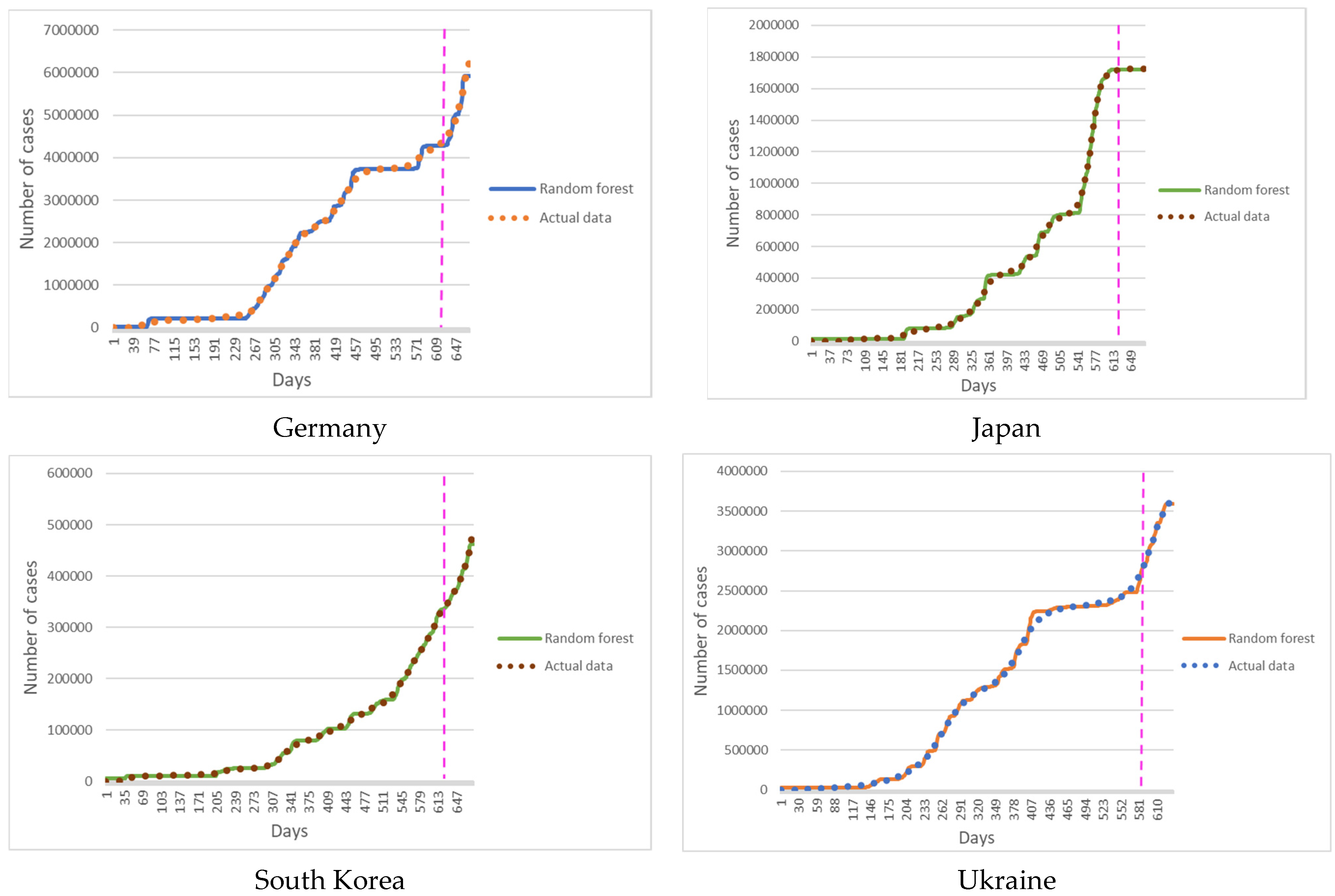
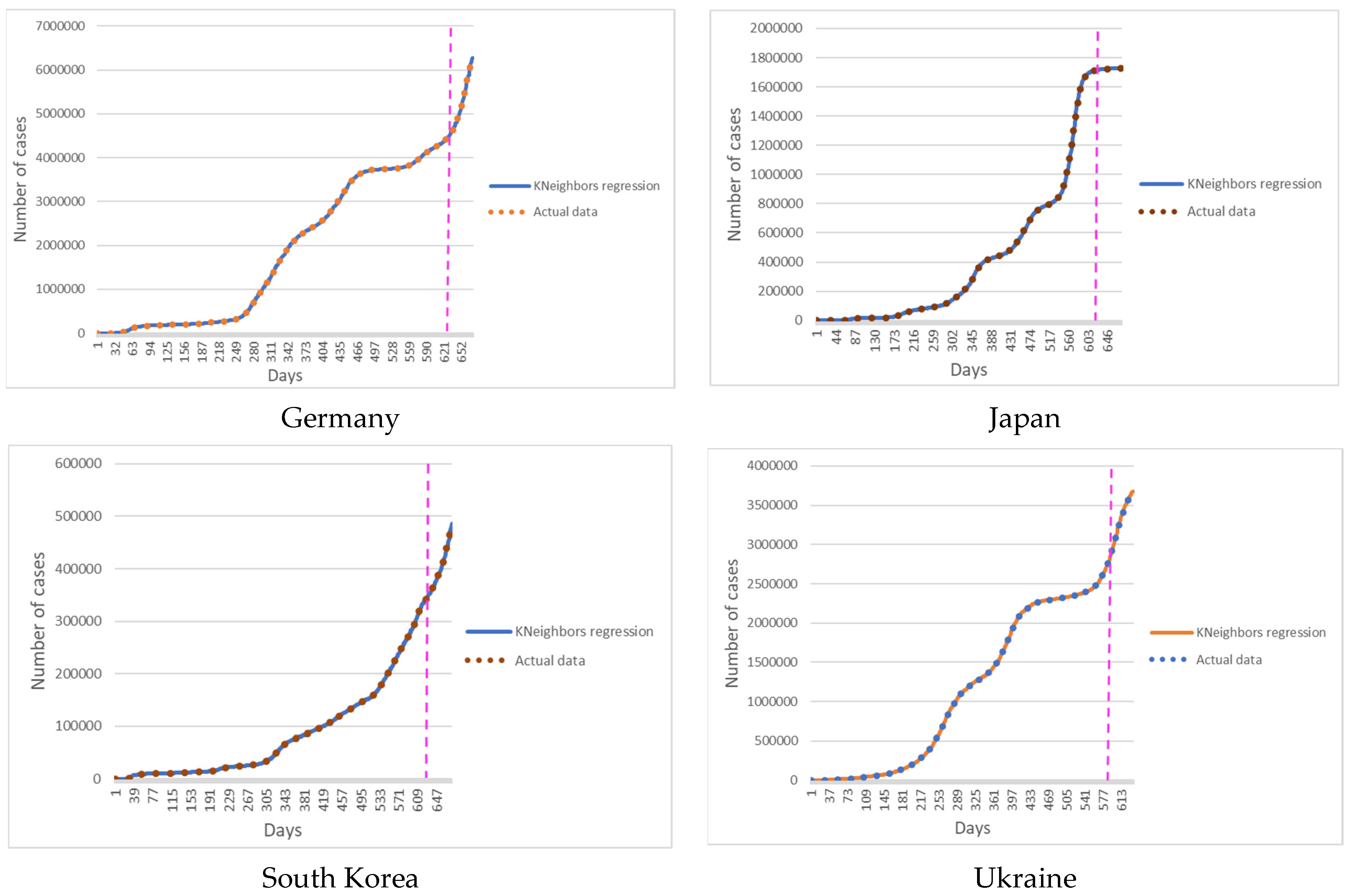
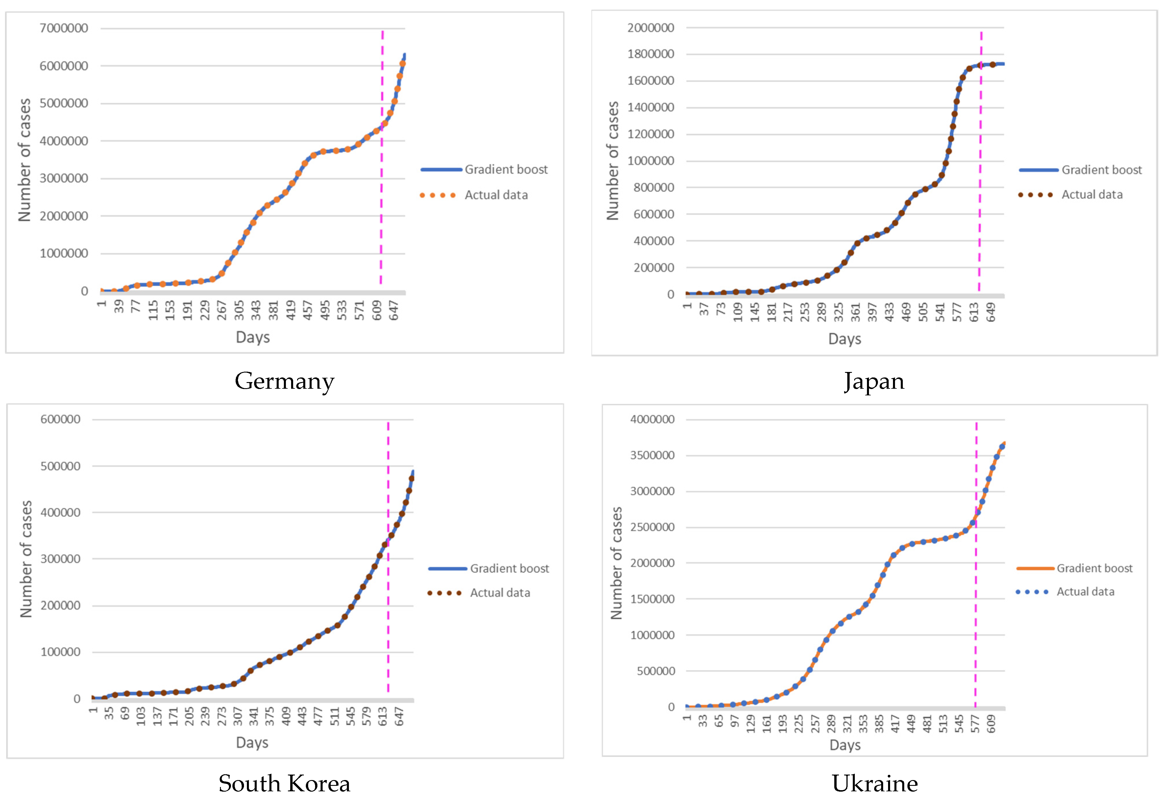
The forecast results show the retrospective dynamics of new cases of COVID-19 in the selected area.

Figure 1 shows the results of predicting new cases of COVID-19 with a Random Forest model. Figure 2 shows the results of predicting new cases of COVID-19 with a K-Nearest Neighbors model. Figure 3 shows the results of predicting new cases of COVID-19 with a Gradient Boosting model. Figure 1, Figure 2 and Figure 3 show the results of simulations for Germany, Japan, South Korea, and Ukraine.

5.2. Forecasting Accuracy Estimation

To assess the accuracy of the models, the relative error and the average absolute error were calculated for the retrospective forecast of the cumulative values of new cases of COVID-19 for the selected territories for 3, 7, 10, 14, 21, and 30 days. The relative error of training data shows the adequacy of the constructed model. The relative error of forecasted data shows the accuracy of the constructed model. However, the error in absolute incidence values is more informative for use in practice by epidemiologists and public health specialists. Absolute incidence rates make it possible to assess the future epidemic situation and take the necessary control measures to contain the epidemic.

Table 1. Relative error of forecasted new cases for Germany (%).

Duration of Forecast (Days)	Random Forest Model	K-Nearest Neighbors Model	Gradient Boosting Model
Training 3	9.409708	0.927918	0.767574
Forecast 3	5.17024	0.544484	0.010204
Training 7	9.45157	0.930967	0.772348
Forecast 7	3.849152	0.473528	0.007183
Training 10	9.49197	0.932761	0.775975
Forecast 10	3.012969	0.491807	0.006026
Training 14	9.534235	0.934895	0.780697
Forecast 14	2.995393	0.517344	0.012878
Training 21	9.615585	0.93961	0.788661
Forecast 21	2.804224	0.510144	0.031779
Training 30	9.737732	0.947268	0.799813
Forecast 30	2.392481	0.474844	0.029858

shows the relative error of developed models for predicting new cases of COVID-19 in Germany.

Table 2. Relative error of forecasted new cases for Japan (%).

Duration of Forecast (Days)	Random Forest Model	K-Nearest Neighbors Model	Gradient Boosting Model
Training 3	49.94565	0.858646	2.272102
Forecast 3	0.441742	0.003262	0.021831
Training 7	50.2621	0.863787	2.286198
Forecast 7	0.430174	0.002863	0.02099
Training 10	50.5022	0.867681	2.296893
Forecast 10	0.421757	0.002989	0.020306
Training 14	50.82606	0.872933	2.311317
Forecast 14	0.410848	0.002813	0.019649
Training 21	51.40349	0.882265	2.337009
Forecast 21	0.388179	0.003121	0.018877
Training 30	52.16673	0.894539	2.370913
Forecast 30	0.351485	0.003791	0.018152

shows the relative error of developed models for predicting new cases of COVID-19 in Japan.

Table 3. Relative error of forecasted new cases for South Korea (%).

Duration of Forecast (Days)	Random Forest Model	K-Nearest Neighbors Model	Gradient Boosting Model
Training 3	5.979816	0.944363	0.427686
Forecast 3	0.97913	0.374233	0.005938
Training 7	6.011627	0.947449	0.430314
Forecast 7	0.991853	0.406392	0.007046
Training 10	6.036437	0.949663	0.432075
Forecast 10	0.952094	0.421965	0.022028
Training 14	6.068961	0.953124	0.434636
Forecast 14	0.966735	0.409796	0.0236
Training 21	6.130652	0.9597	0.439033
Forecast 21	0.869629	0.386758	0.029737
Training 30	6.208069	0.969129	0.444362
Forecast 30	0.891858	0.356536	0.043103

shows the relative error of developed models for predicting new cases of COVID-19 in South Korea.

Table 4. Relative error of forecasted new cases for Ukraine (%).

Duration of Forecast (Days)	Random Forest Model	K-Nearest Neighbors Model	Gradient Boosting Model
Training 3	13.77781	1.313108	0.772439
Forecast 3	1.844497	0.118812	0.010837
Training 7	13.86759	1.32033	0.777511
Forecast 7	1.134243	0.154387	0.011266
Training 10	13.9369	1.326011	0.781295
Forecast 10	0.907004	0.149701	0.015239
Training 14	14.02436	1.333106	0.786291
Forecast 14	1.0065	0.171587	0.022496
Training 21	14.18892	1.345467	0.795291
Forecast 21	0.855615	0.197928	0.025963
Training 30	14.40387	1.361099	0.807296
Forecast 30	0.814586	0.22747	0.025859

shows the relative error of developed models for predicting new cases of COVID-19 in Ukraine.

Table 5. Mean absolute error of forecasted cumulative new cases for Germany (number of cases).

Duration of Forecast (Days)	Random Forest Model	K-Nearest Neighbors Model	Gradient Boosting Model
Forecast 3	323,198.7	34,082.67	639
Forecast 7	238,495.9	29,184.86	445.4286
Forecast 10	185,499.4	29,834.6	370.4
Forecast 14	180,502	107,511	757.2857
Forecast 21	163,443	29,349.67	1748.524
Forecast 30	135,644.6	26,417.57	1598.367

shows the mean absolute error of developed models for predicting cumulative new cases of COVID-19 in Germany.

Table 6. Mean absolute error of forecasted cumulative new cases for Japan (number of cases).

Duration of Forecast (Days)	Random Forest Model	K-Nearest Neighbors Model	Gradient Boosting Model
Forecast 3	7628.333	56.33333	377
Forecast 7	7427.714	49.42857	362.4286
Forecast 10	7281.8	51.6	350.6
Forecast 14	7092.714	52.8765	339.2143
Forecast 21	6700	53.85714	325.8095
Forecast 30	6064.967	65.4	313.2

shows the mean absolute error of developed models for predicting cumulative new cases of COVID-19 in Japan.

Table 7. Mean absolute error of forecasted cumulative new cases for South Korea (number of cases).

Duration of Forecast (Days)	Random Forest Model	K-Nearest Neighbors Model	Gradient Boosting Model
Forecast 3	4518	1731.333	27.33333
Forecast 7	4495.286	1840.714	32
Forecast 10	4258.2	1883.8	96.4
Forecast 14	4249.357	3081.953	101.7143
Forecast 21	3737.238	1659.571	123.7619
Forecast 30	3698.833	1491.267	172.9

shows the mean absolute error of developed models for predicting cumulative new cases of COVID-19 in South Korea.

Table 8. Mean absolute error of forecasted cumulative new cases for Ukraine (number of cases).

Duration of Forecast (Days)	Random Forest Model	K-Nearest Neighbors Model	Gradient Boosting Model
Forecast 3	67,517.67	4343.333	396.6667
Forecast 7	41,389.43	5601.714	409.1429
Forecast 10	33,009.6	5409.4	549.8
Forecast 14	31,624.25	6201.8723	756.23
Forecast 21	30,471.67	6962.619	913
Forecast 30	28,407.57	7791.3	886.5333

shows the mean absolute error of developed models for predicting cumulative new cases of COVID-19 in Ukraine.

5.3. Models Complexity Estimation

Let us estimate the computational complexity of the Random Forest model. When building a model, it has a large size. The complexity of the model is O (NK), where N is the number of trees.

The complexity of training the K-Nearest Neighbors model is O (1). O (n) is technically correct as well. It is needed to remember the training sample. Prediction complexity is O (n) for each feature. If it is required to predict k objects independently using a fixed training sample, then the complexity will be O (kn).

The complexity of the Gradient Boosting model is O (M n log_nd), where M is the number of trees. In general, the model takes longer than a Random Forest because it builds the next tree based on the error or residual of the previous tree, so the process cannot be parallelized compared to a Random Forest.

6. Discussion

It should be noted that COVID-19 refers to infections with an easily possible aerosol transmission mechanism of the pathogen, the source of which is a sick person and a carrier, i.e., an asymptomatic person who sheds a pathogen into the environment and infects other susceptible people. The epidemic process of such infections is significantly influenced by social factors, such as crowding, physical distancing, mask regimen, vaccination coverage of the population, etc. [82]. A step-by-step assessment of the predicted morbidity and its comparison with the registered one allows not only to correctly assess the epidemic situation, the manifestations of the epidemic process characteristic of specific conditions of space and time, but also to assess the quality, effectiveness, and correctness of the preventive and anti-epidemic measures taken, to choose the optimal ones on time and make adjustments as in regulatory documents, and in local preventive action plans.

New challenges for humanity associated with the COVID-19 pandemic forced specialists from various fields of science to mobilize their capabilities. The contribution of specialists in mathematical modeling can be essential for studying the dynamics and characteristics of the manifestations of the epidemic process of emergent infection, the behavior of the pathogen, and the patterns of the spread of the disease are studied simultaneously with the development of preventive and anti-epidemic measures [83]. For a clearer understanding of the patterns of the spread of the COVID-19 pathogen and the choice of the most meaningful and rational measures, we propose evaluating the forecast results through different periods. This information will make it possible to understand the dynamics and features of the epidemic process characteristic of a specific time and a specific territory for which the forecast is made.

The first step is to estimate the expected incidence of COVID-19 after 3 days. The results obtained do not yet allow assessing the correctness of management decisions and the effectiveness of the measures that have been implemented. However, we can understand whether the intensity of the epidemic process has changed compared to the period for which case data were used to build a forecast. Lower rates of predicted morbidity than the actual ones indicate the intensification of the epidemic process and the need to strengthen control measures, which should be paid attention to by decision-makers. The disadvantage of this forecast is that if a period is taken that includes weekends and holidays, then the excess of the predicted incidence compared to the registered one will not reflect the effectiveness of the measures taken. The actual incidence may significantly exceed the registered one [84].

The second step may be to assess the incidence after 7 days. The forecast results after this period allow us to give a preliminary assessment of the correctness of the adopted management decisions. Considering that the average incubation period of COVID-19 is 5–6 days [85], the excess of the actual incidence data of the predicted incidence indicators will roughly give an idea of the need to strengthen control measures, draw the attention of decision-makers to the quality and correctness of the measures that have been developed. An approximate judgment can also be made about the amount of medical care needed for the population. The forecast after 7 days also allows to smooth out the error associated with holidays.

The third step compares the predicted and actual morbidity after 10 days, making it possible to assess the correctness of management decisions more accurately [86]. Fluctuations in incidence associated with weekends and holidays will be leveled. Cases in which infection occurred when the modeling was carried out will be registered. The driving forces of the epidemic process that were in effect for that period (cases with an average incubation period) were taken into account, so those cases that arose after the time when the model was built. New factors could arise or become more active that affect the dynamics and intensity of the COVID-19 epidemic process.

The next step is to assess the incidence in two weeks. 14 days is the maximum incubation period [87]. All cases of infection that occurred at the time of forecasting will already manifest as morbidity or carriage. Comparison of predicted and registered morbidity will allow assessing changes in the dynamics and intensity of the epidemic process, assessing the quality and effectiveness of the measures taken and the correctness of the managerial decisions made, and, if necessary, making adjustments to the volume and content of the control and preventive measures taken. In addition, in two weeks, it is possible to adjust the medical and laboratory network [88]. Exceeding the predicted indicators after 14 days of those indicators registered on the modeling day is a signal for drawing up plans to deploy additional beds for patients, including beds equipped with oxygen, purchase the necessary diagnostic test systems, medicines, and train medical personnel. It is also a signal to strengthen the vaccination campaign in the territory [89].

The next step is to evaluate the forecast data after 21 days. The results allow us to assess the epidemic situation and be a warning for time-taking measures to correct the situation, if necessary. Increasing rates of morbidity growth are a marker for the development of additional measures. You can also preliminarily estimate the required amount of resources—test systems for diagnostics, beds, oxygen stations, medicines, and medical personnel and understand whether the activities included in the plan at the previous stage were sufficient.

Furthermore, finally, the sixth step can be to assess the forecast of incidence in 30 days, which first of all, allows us to assess the burden on the healthcare system, institutions that provide medical care, the required amount of resources and personnel, and the damage from this disease [90]. Estimating the predicted morbidity within this period allows for the taking of necessary advance measures to manage peaks or extreme indicators, such as providing institutions with the necessary resources, and conducting training and retraining of medical personnel, considering the current situation. Other possible strategies include developing the optimal logistics for medical support of both patients and healthy individuals to be vaccinated (organization of vaccination points, providing training of vaccination teams, development of routes, purchase of vaccines, etc.).

To choose a simulation method, one should also consider the possibility of retraining machine learning models. Retraining is characterized by a significant excess of the error value of the test sample of the value of the average error of the training sample. An analysis of the models built in the framework of this study showed that all models are not overfitted.

The minimum number of observations required for a correct result was also analyzed. For a model based on the Random Forest method, the minimum required number of observations is 40, for the Gradient Boosting model—25, for the K-Nearest Neighbors model—15.

7. Conclusions

The paper describes the results of experimental studies of three models based on statistical machine learning methods: Random Forest, K-Nearest Neighbors, and Gradient Boosting. The experiments were performed on new COVID-19 case data provided by the Coronavirus Resource Center of Johns Hopkins University and Medicine for Germany, Japan, South Korea, and Ukraine. These countries were selected because they have different dynamics of the epidemic process and different measures that health systems have implemented to control the pandemic.

All models showed sufficient accuracy in deciding to implement control measures to counter the COVID-19 pandemic. The tasks that can be solved with the help of models depending on the period of the constructed predictive incidence are described.

The prediction accuracy of the Random Forest model is from 94.83% to 99.65%, the K-Nearest Neighbors models are from 99.46% to 99.96%, and the Gradient Boosting models are from 99.97% to 99.99%.

An analysis of the change in the error depending on the forecasting period showed a high agreement between the registered and actual statistics on the incidence of COVID-19 in Japan and South Korea, a satisfactory agreement between the data in Germany, and a low agreement between the registered and actual incidence of COVID-19 in Ukraine. This is due to the completeness of population testing and the testing approaches those countries have implemented during the pandemic.

The scientific novelty of the study lies in the development and study of models of emerging infections using the example of COVID-19 based on simple methods of statistical machine learning. In contrast to other studies, the article analyzes various periods for constructing a forecast, which makes it possible to evaluate the effectiveness of its use for solving various problems of public health.

The practical novelty of the study lies in the implementation of an automated tool for assessing the dynamics of the COVID-19 epidemic process in various territories. It is shown what tasks of epidemiology can be solved when building forecasts for various periods. The accuracy of modeling depends on the completeness of the data of the recorded statistics. Another essential practical value is the ability of public health experts to make decisions based only on new cases of COVID-19. This is especially true for areas where collecting other patient data is not possible due to low funding for the healthcare system or force majeure. For example, in Russia’s war in Ukraine, it is impossible to collect complete data on COVID-19 cases, especially in the temporarily occupied territories and territories where active hostilities are taking place. Under such conditions, the proposed approach will be practical for the timely control of the COVID-19 epidemic process.

Future research development. Despite the high accuracy of the epidemic process models developed in the framework of this study based on statistical machine learning methods, such models do not allow us to identify the factors that affect the development of the epidemic process. It is the identification of factors and assessing their informativity that is an essential task of public health. Therefore, a further development of the study would combine the proposed machine learning models with multi-agent models of epidemic processes. On the one hand, multi-agent models will make it possible to identify and evaluate the factors influencing the dynamics of the epidemic process. On the other hand, machine learning models will improve the accuracy of the predictive incidence of multi-agent models. This will improve the adequacy of experimental studies and the effectiveness of decisions made based on simulation.

References

1. Carvalho, T.; Krammer, F.; Iwasaki, A. The first 12 months of COVID-19: A timeline of immunological insights. Nat. Rev. Immunol. 2021, 21, 245–256. [Google Scholar] [CrossRef] [PubMed]
2. Liu, Q.; Xu, K.; Wang, X.; Wang, W. From SARS to COVID-19: What lessons have we learned? J. Infect. Public Health 2020, 13, 1611–1618. [Google Scholar] [CrossRef] [PubMed]
3. Khan, M.; Adil, S.F.; Alkhathlan, H.Z.; Tahir, M.N.; Saif, S.; Khan, M.; Khan, S.T. COVID-19: A global challenge with old history, epidemiology and progress so far. Molecules 2020, 26, 39. [Google Scholar] [CrossRef] [PubMed]
4. Shih, H.I.; Wu, C.J.; Tu, Y.F.; Chi, C.Y. Fighting COVID-19: A quick review of diagnoses, therapies, and vaccines. Biomed. J. 2020, 43, 341–354. [Google Scholar] [CrossRef]
5. Chen, X.; Gong, W.; Wu, X.; Zhao, W. Estimating economic losses caused by COVID-19 under multiple control measure scenarios with a coupled infectious disease-economic model: A case study in Wuhan, China. Int. J. Environ. Res. Public Health 2021, 18, 11753. [Google Scholar] [CrossRef]
6. Branquinho, C.; Santos, A.C.; Noronha, C.; Ramiro, L.; de Matos, M.G. COVID-19 pandemic and the second lockdown: The 3rd wave of the disease through the voice of youth. Child Indic. Res. 2022, 15, 199–216. [Google Scholar] [CrossRef]
7. Hossain, K.; Hassanzadeganroudsari, M.; Apostolopoulos, V. The emergence of new strains of SARS-CoV-2. What does it mean for COVID-19 vaccines? Expert Rev. Vaccines 2021, 20, 635–638. [Google Scholar] [CrossRef]
8. Brüssow, H. COVID-19: Vaccination problems. Environ. Microbiol. 2021, 23, 2878–2890. [Google Scholar] [CrossRef]
9. Begum, J.; Mir, N.A.; Dev, K.; Buyamayum, B.; Wani, M.Y.; Raza, M. Challenges and prospects of COVID-19 vaccine development based on the progress made in SARS and MERS vaccine development. Transbound. Emerg. Dis. 2021, 68, 1111–1124. [Google Scholar] [CrossRef]
10. Shan, S.G.S.; Nogueras, D.; van Woerden, H.C.; Kiparoglou, V. The COVID-19 pandemic: A pandemic of lockdown loneliness and the role of digital technology. J. Med. Internet Res. 2020, 22, e22287. [Google Scholar] [CrossRef]
11. Fedorovich, O.; Uruskiy, O.; Pronchakov, Y.; Lukhanin, M. Method and information technology to research the component architecture of products to justify investments of high-tech enterprise. Radioelectron. Comput. Syst. 2021, 1, 150–157. [Google Scholar] [CrossRef]
12. Agosto, A.; Giudici, P. COVID-19 contagion and digital finance. Digit. Financ. 2020, 2, 159–167. [Google Scholar] [CrossRef] [PubMed]
13. Fedushko, S.; Ustyianovych, T. E-commerce customers behavior research using cohort analysis: A case study of COVID-19. J. Open Innov. Technol. Mark. Complex. 2022, 8, 12. [Google Scholar] [CrossRef]
14. Davidich, N.; Chumachenko, I.; Davidich, Y.; Hanieva, T.; Artsybasheva, N.; Melenchuk, T. Advanced traveller information systems to optimizing freight driver route selection. In Proceedings of the 2020 13th International Conference on Developments in eSystems Engineering (DeSE), Liverpool, UK, 14–17 December 2020; pp. 111–115. [Google Scholar] [CrossRef]
15. Misiuk, T.; Kondratenko, Y.; Sidenko, I.; Kondratenko, G. Computer vision mobile system for education using augmented reality technology. J. Mob. Multimed. 2021, 17, 555–576. [Google Scholar]
16. Nechyporenko, A.; Reshetnik, V.; Shyian, D.; Yurevych, N.; Alekseeva, V.; Nazaryan, R.; Gargin, V. Comparative characteristics of the anatomical structures of the ostiomeatal complex obtained by 3D modeling. In Proceedings of the 2020 IEEE International Conference on Problems of Infocommunications Science and Technology, Kharkiv, Ukraine, 6–9 October 2021; pp. 407–411. [Google Scholar] [CrossRef]
17. Bazilevych, K.; Krivtsov, S.; Butkevych, M. Intelligent evaluation of the informative features of cardiac studies diagnostic data using Shannon method. CEUR Workshop Proc. 2021, 3003, 65–75. [Google Scholar]
18. Izonin, I.; Tkachenko, R.; Verhun, V.; Zub, K. An approach towards missing data management using improved GRNN-SGTM ensemble method. Eng. Sci. Technol. 2021, 24, 749–759. [Google Scholar] [CrossRef]
19. Yakovlev, S.; Bazilevych, K.; Chumachenko, D.; Chumachenko, T.; Hulianytskyi, L.; Meniailov, I.; Tkachenko, A. The concept of developing a decision support system for the epidemic morbidity control. CEUR Workshop Proc. 2020, 2753, 265–274. [Google Scholar]
20. Ross, R. An application of the theory of probabilities to the study of a priori pathometry. Proc. R. Soc. Lond. 1916, 92, 204–230. [Google Scholar] [CrossRef] [Green Version]
21. Hamer, W. The Milroy lectures. On epidemic disease in England—The evidence of variability and of persistency of type. Lancet 1906, 167, 569–574. [Google Scholar] [CrossRef]
22. Kermack, W.O.; McKendrick, A.G. Contribution to the mathematical theory to epidemics. Proc. R. Soc. Lond. 1927, 115, 700–721. [Google Scholar] [CrossRef] [Green Version]
23. Holz, M.; Fahr, A. Compartment modeling. Adv. Drug Deliv. Rev. 2001, 48, 249–264. [Google Scholar] [CrossRef]
24. Kuddus, A.; Mohiuddin, M.; Rahman, A. Mathematical analysis of a measles transmission dynamics model in Bangladesh with double dose vaccination. Sci. Rep. 2021, 11, 16571. [Google Scholar] [CrossRef] [PubMed]
25. Ostus, D.; Hickmann, K.S.; Caragea, P.C.; Higdon, D.; del Valle, S.Y. Forecasting seasonal influenza with a state-space SIR model. Ann. Appl. Stat. 2017, 11, 202–224. [Google Scholar] [CrossRef] [PubMed]
26. Baroyan, O.V.; Rvachev, L.A. Deterministic models of epidemics for a territory with a transport network. Cybern. Syst. Snalysis 1967, 3, 55–61. [Google Scholar] [CrossRef]
27. Rihan, F.A.; Baleanu, D.; Lakshmanan, S.; Rakkiyappan, R. On fractional SIRC model with Salmonella bacterial infection. Abstr. Appl. Anal. 2014, 2014, 136263. [Google Scholar] [CrossRef] [Green Version]
28. Van Effelterre, T.P.; Zink, T.K.; Hoet, B.J.; Hausdorff, W.P.; Rosenthal, P. A mathematical model of Hepatitis A transmission in the United States indicates value of universal childhood immunization. Clin. Infect. Dis. 2006, 43, 158–164. [Google Scholar] [CrossRef]
29. Islam, Z.; Ahmed, S.; Rahman, M.M.; Karim, M.F.; Amin, M.R. Global stability and parameter estimation for a diphtheria model: A case study of an epidemic in Rohingya refugee camp in Bangladesh. Comput. Math. Methods Med. 2022, 2022, 6545179. [Google Scholar] [CrossRef]
30. Huo, H.F.; Chen, R.; Wang, X.Y. Modelling and stability of HIV/AIDS epidemic model with treatment. Appl. Math. Model. 2016, 40, 6550–6559. [Google Scholar] [CrossRef]
31. Khan, M.A.; Islam, S.; Arif, M.; ul Haq, Z. Transmission model of Hepatitis B virus with the migration effect. BioMed Res. Int. 2013, 2013, 150681. [Google Scholar] [CrossRef]
32. Stocks, T.; Martin, L.J.; Kuhlmann-Berenzon, S.; Britton, T. Dynamic modeling of Hepatitis C transmission among people who inject drugs. Epidemics 2020, 30, 100378. [Google Scholar] [CrossRef] [PubMed]
33. Brown, R.A. A simple model for control of COVID-19 infections on an urban campus. Proc. Natl. Acad. Sci. USA 2021, 118, e2105292118. [Google Scholar] [CrossRef] [PubMed]
34. Zha, J.; Liu, X.; Sui, M. The SEIR model of COVID-19 forecasting rates of infections in New York city. J. Phys. Conf. Ser. 2021, 1735, 012009. [Google Scholar] [CrossRef]
35. Radulescu, A.; Williams, C.; Cavanagh, K. Management strategies in a SEIR-type model of COVID-19 community spread. Sci. Rep. 2020, 10, 21256. [Google Scholar] [CrossRef] [PubMed]
36. Erandi, K.K.W.H.; Mahasinghe, A.C.; Perera, S.S.N.; Jayasinghe, S. Effectiveness of the strategies implemented in Sri Lanka for controlling the COVID-19 outbreak. J. Appl. Math. 2020, 2020, 2954519. [Google Scholar] [CrossRef]
37. Alexandrou, C.; Harmandaris, V.; Irakleous, A.; Koutsou, G.; Savva, N. Modeling the evolution of COVID-19 via compartmental and particle-based approaches: Application to the Cyprus case. PLoS ONE 2020, 16, e0250709. [Google Scholar] [CrossRef] [PubMed]
38. Forien, R.; Pang, G.; Pardoux, E. Estimating the state of the COVID-19 epidemic in France using a model with memory. R. Soc. Open Sci. 2021, 8, 202327. [Google Scholar] [CrossRef]
39. Nistal, R.; de la Sen, M.; Gabirondo, J.; Alonso-Quesada, S.; Garrido, A.J.; Garrido, I. A Study on COVID-19 Incidence in Europe through Two SEIR Epidemic Models Which Consider Mixed Contagions from Asymptomatic and Symptomatic Individuals. Appl. Sci. 2021, 11, 6266. [Google Scholar] [CrossRef]
40. Cooped, I.; Mondal, A.; Antonopoulos, C.G. A SIR model assumption for the spread of COVID-19 in difference communities. Chaos Solut. Fractals 2020, 139, 110057. [Google Scholar] [CrossRef]
41. Al-Raeei, M.; El-Daher, M.S.; Solieva, O. Applying SEIR model without vaccination for COVID-19 in case of the United States, Russia, the United Kingdom, Brazil, France, and India. Epidemiol. Methods 2021, 10, 20200036. [Google Scholar] [CrossRef]
42. Odagaki, T. Exact properties of SIQR model for COVID-19. Phys. A 2021, 564, 125564. [Google Scholar] [CrossRef]
43. Mugdha, S.B.S.; Uddin, M.; Islam, T. Extended epidemiological models for weak economic region: Case studies of the spreading of COVID-19 in the South Asian subcontinental countries. BioMed Res. Int. 2021, 2021, 7787624. [Google Scholar] [CrossRef] [PubMed]
44. Rahimi, I.; Gandomi, A.H.; Asteris, P.G.; Chen, F. Analysis and Prediction of COVID-19 Using SIR, SEIQR, and Machine Learning Models: Australia, Italy, and UK Cases. Information 2021, 12, 109. [Google Scholar] [CrossRef]
45. Franco, N. COVID-19 Belgium: Extended SEIR-QD model with nursing homes and long-term scenarios-based forecasts. Epidemics 2021, 37, 100490. [Google Scholar] [CrossRef] [PubMed]
46. Ghostine, R.; Gharamti, M.; Hassrouny, S.; Hoteit, I. An Extended SEIR Model with Vaccination for Forecasting the COVID-19 Pandemic in Saudi Arabia Using an Ensemble Kalman Filter. Mathematics 2021, 9, 636. [Google Scholar] [CrossRef]
47. Gorbachuk, V.M.; Dunaievskyi, M.S.; Syrku, A.A.; Suleimanov, S.B. Substantiating the diffusion model of innovation implementation and its application to vaccine propagation. Cybern. Syst. Anal. 2022, 58, 84–94. [Google Scholar] [CrossRef]
48. Guan, L.; Prieur, C.; Zhang, L.; Prieur, C.; Georges, D.; Bellemain, P. Transport effect of COVID-19 pandemic in France. Annu. Rev. Control 2020, 50, 394–408. [Google Scholar] [CrossRef]
49. Putra, Z.A.; Abidin, S.A.Z. Application of SEIR model in COVID-19 and the effect of lockdown on reducing the number of active cases. Indones. J. Sci. Technol. 2020, 5, 10–17. [Google Scholar] [CrossRef]
50. Dashtbali, M.; Mirzaie, M. A compartmental model that predicts the effect of social distancing and vaccination on controlling COVID-19. Sci. Rep. 2021, 11, 8191. [Google Scholar] [CrossRef]
51. Morciglio, A.; Zhang, B.; Chowell, G.; Hyman, J.M.; Jiang, Y. Mask-Ematics: Modeling the Effects of Masks in COVID-19 Transmission in High-Risk Environments. Epidemiologia 2021, 2, 207–226. [Google Scholar] [CrossRef]
52. Asamoah, J.K.K.; Jin, Z.; Sun, G.Q.; Seidu, B.; Yankson, E.; Abidemi, A.; Oduro, F.T.; Moore, S.E.; Okyere, E. Sensitivity assessment and optimal economic evaluation of a new COVID-19 compartmental epidemic model with control interventions. Chaos Solut. Fractals 2021, 146, 110885. [Google Scholar] [CrossRef]
53. Masandawa, L.; Mirau, S.S.; Mbalawata, I.S. Mathematical modeling of COVID-19 transmission dynamics between healthcare workers and community. Results Phys. 2021, 29, 104731. [Google Scholar] [CrossRef] [PubMed]
54. Jen, G.H.H.; Chen, S.Y.; Chang, W.J.; Chen, C.N.; Yen, A.M.F.; Chang, R.E. Evaluating medical capacity for hospitalization and intensive care unit of COVID-19: A queue model approach. J. Formos. Med. Assoc. 2021, 120 (Suppl. S1), S86–S94. [Google Scholar] [CrossRef]
55. Dong, E.; Du, H.; Gardner, L. An interactive web-based dashboard to track COVID-19 in real time. Lancet Infect. Dis. 2020, 20, 533–534. [Google Scholar] [CrossRef]
56. Robert Koch-Institut: COVID-19 Dashboard. 2020. Available online: https://experience.arcgis.com/experience/478220a4c454480e823b17327b2bf1d4 (accessed on 25 April 2022).
57. Schilling, J.; Tolksdorf, K.; Marquis, A.; Faber, M.; Pfoch, T.; Buda, S.; Haas, W.; Schuler, E.; Altmann, D.; Grote, U.; et al. Die verschiedenen Phasen der COVID-19-Pandemie in Deutschland: Eine deskriptive Analyse von Januar 2020 bis Februar 2021. Bundesgesundheitsblat—Gesundh. Gesundh. 2021, 64, 1093–1106. [Google Scholar] [CrossRef] [PubMed]
58. Braun, P. Effect of lockdown and vaccination on the course of the COVID-19 pandemic in Germany. Int. J. Clin. Pharmacol. Ther. 2022, 60, 125–135. [Google Scholar] [CrossRef]
59. Bittmann, S. Role of Omicron variant of SARS-CoV-2 in children in Germany. World J. Pediatrics 2022, 18, 283–284. [Google Scholar] [CrossRef]
60. Gandjour, A. How Many Intensive Care Beds are Justifiable for Hospital Pandemic Preparedness? A Cost-effectiveness Analysis for COVID-19 in Germany. Appl. Health Econ. Health Policy 2021, 19, 181–190. [Google Scholar] [CrossRef]
61. Leithauser, N.; Schneider, J.; Johann, S.; Krumke, S.O.; Schmidt, E.; Streicher, M.; Scholz, S. Quantifying Covid19-vaccine location strategies for Germany. BMC Health Serv. Res. 2021, 21, 780. [Google Scholar] [CrossRef]
62. Hara, Y.; Yamaguchi, H. Japanese travel behavior trends and change under COVID-19 state-of-emergency declaration: Nationwide observation by mobile phone location data. Transp. Res. Interdiscip. Perspect. 2021, 9, 100288. [Google Scholar] [CrossRef]
63. Ishikawa, Y.; Hifumi, T.; Urashima, M. Critical care medical centers may play an important role in reducing the risk of COVID-19 death in Japan. SN Compr. Clin. Med. 2020, 2, 2147–2150. [Google Scholar] [CrossRef]
64. Wu, Y.C.; Chen, C.S.; Chan, Y.J. The outbreak of COVID-19: An overview. J. Chin. Med. Assoc. 2020, 83, 217–220. [Google Scholar] [CrossRef] [PubMed]
65. Liu, S.; Yamamoto, T. Role of stay-at-home requests and travel restrictions in preventing the spread of COVID-19 in Japan. Transp. Res. Part A Policy Pract. 2022, 159, 1–16. [Google Scholar] [CrossRef] [PubMed]
66. Machida, M.; Nakamura, I.; Kojima, T.; Saito, R.; Nakaya, T.; Hanibuchi, T.; Takamiya, T.; Odagiri, Y.; Fukushima, N.; Kikuchi, H.; et al. Acceptance of a COVID-19 vaccine in Japan during the COVID-19 pandemic. Vaccines 2021, 9, 210. [Google Scholar] [CrossRef] [PubMed]
67. Kim, H. COVID-19 Apps as a digital intervention police: A longitudinal panel data analysis in South Korea. Health Policy 2021, 125, 1430–1440. [Google Scholar] [CrossRef]
68. Kim, N.; Kang, S.J.; Tak, S. Reconstructing a COVID-19 outbreak within a religious group using social network analysis simulation in Korea. Epidemiol. Health 2021, 43, e2021068. [Google Scholar] [CrossRef]
69. Lee, D.; Heo, K.; Seo, Y.; Ahn, H.; Jung, K.; Lee, S.; Choi, H. Flattening the curve on COVID-19: South Korea’s measures in tackling initial outbreak of Coronavirus. Am. J. Epidemiol. 2021, 190, 496–505. [Google Scholar] [CrossRef]
70. Kim, Y.J.; Sung, H.; Ki, C.S.; Hur, M. COVID-19 testing in South Korea: Current status and the need for faster diagnostics. Ann. Lab. Med. 2020, 40, 349–350. [Google Scholar] [CrossRef]
71. Choi, Y.; Kim, J.S.; Kim, J.E.; Choi, H.; Lee, C.H. Vaccination prioritization strategies for COVID-19 in Korea: A mathematical modeling approach. Int. J. Environ. Res. Public Health 2021, 18, 4240. [Google Scholar] [CrossRef]
72. Gankin, Y.; Nemira, A.; Koniukhovskii, V.; Chowell, G.; Weppelmann, T.A.; Skums, P.; Kirpich, A. Investigating the first stage of the COVID-19 pandemic in Ukraine using epidemiological and genomic data. Infect. Genet. Evol. J. Mol. Epidemiol. Evol. Genet. Infect. Dis. 2021, 95, 105087. [Google Scholar] [CrossRef]
73. Ivats-Chabina, A.R.; Korolchuk, O.L.; Kachur, A.Y.; Smiianov, V.A. Healthcare in Ukraine during the pandemic: Difficulties, challenges and solutions. Wiad. Lek. 2021, 74, 1256–1261. [Google Scholar] [CrossRef]
74. Patel, S.S.; Moncayo, O.E.; Conroy, K.M.; Jordan, D.; Erickson, T.B. The landscape of disinformation of health crisis communication during the COVID-19 pandemic in Ukraine: Hybrid warfare tactics, fake media news and review of evidence. J. Sci. Commun. 2020, 19, AO2. [Google Scholar] [CrossRef] [PubMed]
75. Matiashova, L.; Isayeva, G.; Shanker, A.; Tsagkaris, C.; Aborode, A.T.; Essar, M.Y.; Ahmad, S. COVID-19 vaccination in Ukraine: An update on the status of vaccination and the challenges at hand. J. Med. Virol. 2021, 93, 5252–5253. [Google Scholar] [CrossRef] [PubMed]
76. Guerard, J.B. Regression analysis and forecasting models. In Introduction to Financial Forecasting in Investment Analysis; Springer: New York, NY, USA, 2013. [Google Scholar] [CrossRef]
77. Svetnik, V.; Liaw, A.; Tong, C.; Culberson, J.C.; Sheridan, R.P.; Feuston, B.P. Random Forest: A classification and regression tool for compound classification and QSAR modeling. J. Chem. Inf. Comput. Sci. 2003, 43, 1947–1958. [Google Scholar] [CrossRef] [PubMed]
78. Kumar, T. Solution of linear and non linear regression problem by K Nearest Neighbour approach: By using three sigma rule. In Proceedings of the 2015 IEEE International Conference on Computational Intelligence & Communication Technology, Ghaziabad, India, 13–14 February 2015; pp. 197–201. [Google Scholar] [CrossRef]
79. Singh, U.; Rizwan, M.; Alaraj, M.; Alsaidan, I. A machine learning-based gradient boosting regression approach for wind power production forecasting: A step towards smart grid environments. Energies 2021, 14, 5196. [Google Scholar] [CrossRef]
80. Chen, C.; Twycross, J.; Garibaldi, J.M. A new accuracy measure based on bounded relative error for time series forecasting. PLoS ONE 2017, 12, e0174202. [Google Scholar] [CrossRef] [Green Version]
81. Willmott, C.J.; Matsuura, K. Advantages of the mean absolute error (MAE) over the root mean square error (RMSE) in assessing average model performance. Clim. Res. 2005, 30, 79–82. [Google Scholar] [CrossRef]
82. Seligman, B.; Ferranna, M.; Bloom, D.E. Social determinants of mortality from COVID-19: A simulation study using NHANES. PLoS Med. 2021, 18, e1003490. [Google Scholar] [CrossRef]
83. Rubin, D.M.; Achari, S.; Carlson, C.S.; Letts, R.F.R.; Pantanowitz, A.; Postema, M.; Richards, X.L.; Wigdorowitz, B. Facilitating understanding, modeling and simulation of infectious disease epidemics in the age of COVID-19. Front. Public Health 2021, 9, 593417. [Google Scholar] [CrossRef]
84. Wiwanitkit, V.; Joob, B. Density of COVID-19 and mass population movement during long holiday: Simulation comparing between using holiday postponement and no holiday postponement. J. Res. Med. Sci. Off. J. Isfahan Univ. Med. Sci. 2020, 25, 55. [Google Scholar] [CrossRef]
85. Lauer, A.S.; Grantz, K.H.; Bi, Q.; Jones, F.K.; Zheng, Q.; Meredith, H.R.; Azman, A.S.; Reich, N.G.; Lessler, J. The incubation period of coronavirus disease 2019 (COVID-19) from publicly reported confirmed cases: Estimation and application. Ann. Intern. Med. 2020, 172, 577–582. [Google Scholar] [CrossRef] [Green Version]
86. Chen, Y.; Li, Q.; Karimian, H.; Chen, X.; Li, X. Spatio-temporal distribution characteristics and influencing factors of COVID-19 in China. Sci. Rep. 2021, 11, 3717. [Google Scholar] [CrossRef] [PubMed]
87. Leung, C. The incubation period of COVID-19: Current understanding and modeling technique. Adv. Exp. Med. Biol. 2021, 1318, 81–90. [Google Scholar] [CrossRef] [PubMed]
88. Zeinalnezhad, M.; Chofreh, A.G.; Goni, F.A.; Klemes, J.J.; Sari, E. Simulation and improvement of patients’ workflow in heart clinics during COVID-19 pandemic using timed coloured Petri nets. Int. J. Environ. Res. Public Health 2020, 17, 8577. [Google Scholar] [CrossRef] [PubMed]
89. Karabay, A.; Kuzdeuov, A.; Varol, H.A. COVID-19 vaccination strategies considering hesitancy using particle-based epidemic simulation. In Proceedings of the Annual International Conference of the IEEE Engineering in Medicine and Biology Society, Mexico, online, 1–5 November 2021; pp. 1985–1988. [Google Scholar] [CrossRef]
90. Bayraktar, Y.; Ozyilmaz, A.; Toprak, M.; Isik, E.; Buyukakin, F.; Olgun, M.F. Role of the health system in combating COVID-19: Cross-section analysis and artificial neural network simulation for 124 country cases. Soc. Work Public Health 2021, 36, 178–193. [Google Scholar] [CrossRef] [PubMed]
Figure 1. Forecasting of COVID-19 new cases by Random Forest model.
Computation 10 00086 g001
Figure 2. Forecasting of COVID-19 new cases by K-Nearest Neighbors model.
Computation 10 00086 g002
Figure 3. Forecasting of COVID-19 new cases by Gradient Boosting model.
Computation 10 00086 g003