
Cluster-Based Analogue Ensembles for Hindcasting with Multistations


1
Research Centre in Digitalization and Intelligent Robotics (CeDRI), Instituto Politécnico de Bragança, 5300-253 Bragança, Portugal
2
Vestas Wind Systems A/S, Vestas Technology Centre Porto, 4465-671 Leça do Balio, Portugal
3
Universidade Tecnológica Federal do Paraná, Campus de Ponta Grossa, Ponta Grossa 84017-220, Brazil
*
Author to whom correspondence should be addressed.
†
These authors contributed equally to this work.
Computation 2022, 10(6), 91; https://0-doi-org.brum.beds.ac.uk/10.3390/computation10060091
Submission received: 29 April 2022
/
Revised: 20 May 2022
/
Accepted: 27 May 2022
/
Published: 2 June 2022
(This article belongs to the Special Issue Applications of Computational Mathematics to Simulation and Data Analysis)
Abstract
:The Analogue Ensemble (AnEn) method enables the reconstruction of meteorological observations or deterministic predictions for a certain variable and station by using data from the same station or from other nearby stations. However, depending on the dimension and granularity of the historical datasets used for the reconstruction, this method may be computationally very demanding even if parallelization is used. In this work, the classical AnEn method is modified so that analogues are determined using K-means clustering. The proposed combined approach allows the use of several predictors in a dependent or independent way. As a result of the flexibility and adaptability of this new approach, it is necessary to define several parameters and algorithmic options. The effects of the critical parameters and main options were tested on a large dataset from real-world meteorological stations. The results show that adequate monitoring and tuning of the new method allows for a considerable improvement of the computational performance of the reconstruction task while keeping the accuracy of the results. Compared to the classical AnEn method, the proposed variant is at least 15-times faster when processing is serial. Both approaches benefit from parallel processing, with the K-means variant also being always faster than the classic method under that execution regime (albeit its performance advantage diminishes as more CPU threads are used).
1. Introduction
Short-term weather predictions by correlation with similar states in the past (analogues) were originally established by Lorenz [1], who suggested that two atmospheric states that are initially very close to each other will remain somewhat similar in the future. This was introduced as an alternative to classical weather forecasting based on systems of equations underlying deterministic Numerical Weather Prediction (NWP) models.
For many years, however, Lorenz’s proposal was discarded because of limited historical data on past weather conditions (especially over wide geographical areas) and insufficient computing capacity to implement his approach. Two decades later, van den Dool [2] revisited analogue-based short-range weather forecasting and found it to be feasible and effective when applied to limited geographical areas.
Monache [3] showed the applicability of an analogue scheme (named AN) for post-processing numerical weather forecasts to reduce systematic and random errors. The basic idea is that if previous forecasts (analogues) exist that are similar to the current NWP forecast (predictor), it is possible to produce a AN forecast by averaging the observations corresponding to these previous forecasts. The analogue prediction is then compared with the NWP prediction to infer the prediction error and thus improve the NWP forecast.
Later, Monache refined the use of analogues to estimate the probability distribution of the future state of the atmosphere [4]. Instead of focusing on improving a single deterministic NWP prediction, the goal was to derive a Probability Density Function (PDF) of the range of possible future states (forecasts)—a more realistic approach due to imperfect initial conditions and model limitations that generate prediction errors. In the same paper, the term analogue ensemble (AnEn) was coined to refer to both the observations that correspond to past analogue predictions and the method used to select these observations.
Since its introduction, the AnEn method has gained traction in many contexts, e.g., renewable energy management—in particular, wind and solar energy forecasting [5,6]. It has also been combined with other approaches, such as artificial neural networks, e.g., for predicting the power generated by photovoltaic power plants [7].
Studies aiming at the development of AnEn techniques favour applications in downscaling and forecasting rather than hindcasting, yet all topics share affinities. In the area of downscaling, we highlight the study conducted by Rozoff and Alessandrini comparing AnEn with convolutional neural networks (CNNs) for reconstructing high-resolution 10 m winds over complex terrain, where AnEn was found to produce lower errors than CNNs [8].
In the field of forecasting, AnEn is mainly used for the post-processing of forecast results. In recent years, post-processing with AnEn has been applied to the prediction of a wide range of meteorological variables and energy. For example, the AnEn technique has been used to improve the accuracy of ozone and particulate matter forecasts [9]. Solar forecasting, which involves the prediction of irradiance and solar power forecasting, has also attracted considerable attention in the last decade [10].
Among all post-processing forecast applications, there is a consensus that AnEn benefits from increasingly large training datasets. However, the large amount of data that must be processed to determine the analogues often makes the computational cost prohibitive [11]. Thus, there is a great interest in improving the computational efficiency of the AnEn method. One of the major outcomes of this interest was the development of the Parallel Analogue Ensemble (PAnEn) library [12]. This library, which provides an efficient parallel implementation of the AnEn method and user-friendly interfaces in R and C++, has been successfully applied to a huge dataset related to photovoltaic power generation [13].
This study aims to improve the computational efficiency of the AnEn method, not with the focus on the parallelization of the original algorithm but by reducing the number of operations required to compute the analogues, which is the most demanding task. The various computational loops needed to determine the analogue ensembles were replaced by a single step that employs clustering through the K-means method.
This new approach was developed in the field of hindcasting. Since this field has many similarities with downscaling and forecasting, the proposed cluster-based variant of the AnEn method could be easily adapted to these fields. Furthermore, the algorithm of the new approach is presented in detail. The effects of its most important parameters are examined with regard to the reliability and computational efficiency of the method.
This work is a revised and extended version of [14]. It provides a more complete mathematical and algorithmic formulation of the classical and K-means-based AnEn method. A complete characterization of the dataset used is given. The influence of additional method parameters is also investigated. The computational performance results cover a broader scenario of parallel execution and additional performance metrics are presented.
In the following, Section 2 reviews the classical AnEn method in the context of hindcasting; Section 3 formally presents the different ways of selecting analogues for the different approaches investigated in this work; Section 4 presents the meteorological dataset and the error metrics used to validate the predictions; Section 5 provides the numerical results obtained for different values of the main parameters of the K-means-based AnEn method; Section 6 is devoted to the comparison of the computational performance of the proposed method with the classical one; Section 7 finally concludes with an outlook on future work.
2. Hindcasting with the AnEn Method
The AnEn method plays an important role in weather hindcasting. Classically, weather hindcasting involves applying a forecast model to a past starting point to validate the model by comparing its forecasts with available observations (reanalysis). If some observations are not available, their time-series can be complemented (reconstruction) by using the corresponding forecasts as a substitute for the missing observations. However, the combination of hindcasting with the AnEn method also makes it possible to reconstruct meteorological data. For example, a variable at a meteorological station can be reconstructed based on the data of correlated variables from the same station or/and from other nearby stations.
The last option, known as hindcasting with multistations, was explored in previous work [15]. There, cosine similarity, normalization and K-means clustering were used as similarity metrics for analogue selection, as an alternative to the classical Monache metric. The coupling of the AnEn method with K-means clustering proved to be promising. At the same time, the results suggested the need to consider other clustering methods and to conduct a parametric study on important parameters of the methods under consideration.
Such study was initiated in [16] in the context of reconstructing a single meteorological variable. The study restricted the choice of analogues to the classical Monache metric, the K-means and the C-means clustering methods and confirmed that K-means provides the best accuracy. Heuristics were also identified for determining the number of clusters, the number of analogues and the analogue time span, which minimized the prediction errors.
Recently, the combination of K-means clustering with the AnEn method was further investigated in [14]. The mathematical formulation of the resulting approach was introduced to emphasize the important options and parameters of the new method. A parametric study was conducted in the context of the hindcasting of extra meteorological variables from the same dataset used in [16]. The computational performance of the K-means-based and classical AnEn methods were compared for a limited parallel execution scenario.
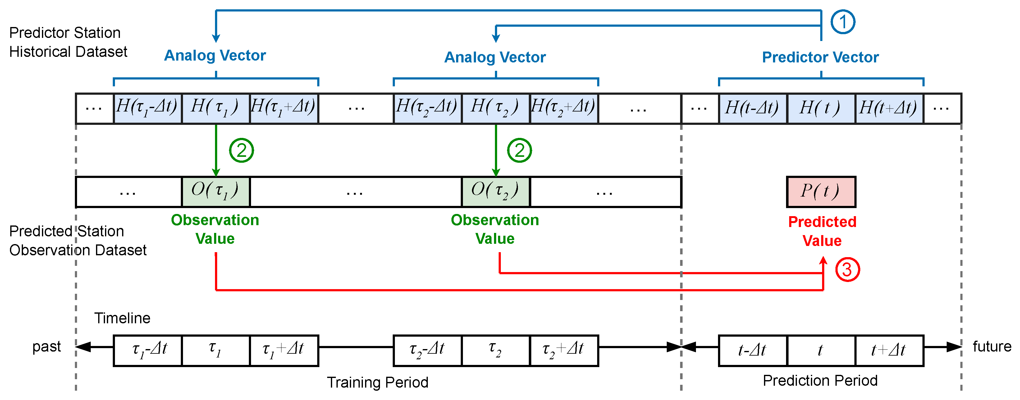
The application of the AnEn method to the reconstruction of missing data, from time-series of real-world observations, is illustrated by Figure 1, for the scenario of a single predictor station. In the figure, the historical dataset is a full record of past observations of a certain meteorological variable collected at the predictor station, and the observation dataset is an incomplete record of the same or a correlated variable at the predicted station (this record is complete for a training period but incomplete or absent for a prediction period).
The reconstruction of a missing value (predicted value) of the predicted station, concerning a certain instant t in time, unfolds in three different steps.
In step ①, a certain number of analogues are selected from the historical dataset based on the similarity of the past observations to a predictor at instant t. Both the predictor and each analogue are vectors of elements sampled at successive intervals of time-step. Each element is the value of a meteorological variable and k is a positive integer that represents the width of each half-window (into the past and future) around the central instant of the time window ( in the scenario of Figure 1). Comparing vectors instead of single values considers the evolutionary trend of the meteorological variable around the central instant of the time window, allowing for the selection of analogues to be based on short-range weather patterns instead of single isolated events.
In step ②, the analogue map onto observations in the training period of the predicted station. This mapping is done only for the central instant of the analogue time window, meaning that, for each analogue vector, only a single observational value is selected.
Finally, in step ③, the observations selected are used to estimate the missing predicted value. If this value is indeed available as real observational data (as assumed in this paper), it then becomes possible to assess the prediction/reconstruction error.
In this work, the methodology described above is combined with K-means clustering as an alternative way of defining the set of analogues. In the ensuing text, the following notation is used: H stands for the historical time-series from where analogues are defined, O represents the measurements/observations time-series for the feature to be predicted, and P is the outcome prediction. Whilst O and P can be viewed solely as function of time t, when using multistations the history H will be an aggregate of time-series of multiple predictor stations, in which case, it will be a function also of the station s—that is, .
3. Searching for Analogue Ensembles
This section presents the techniques that are relevant in the scope of this work to find analogues. It begins with the classical error-based approaches and ends with the proposed cluster-based technique (for which a complete formal description is provided).
3.1. Classical Error-Based Analogues
The classical techniques are based on the score obtained through given error metrics (). These metrics differ depending on the predictor stations being used in an independent or dependent way: in the first scenario, the choice of analogues for a predictor station is independent of the choice made for other predictor stations; in the second scenario, the analogues chosen for the different predictor stations must coincide in time.
3.1.1. Independent Analogues
With a single predictor station, a univariate similarity metric can be defined [3] as
where H is a single historical time-series from where analogues are chosen, t is a time instant in the prediction period of H, is a time instant defining a possible analogue in the training period of H, and is the time-series time-step. Both t and are the central instants of time windows with consecutive instants that are apart in time. For each time window, there is a vector with consecutive records of a meteorological variable. The metric is a Euclidean distance between a possible analogue and the predictor, such that the best analogues are those that yield the lowest values (scores) of . This metric can be adapted to a scenario with multiple predictor stations at different locations, identified by an index s, each with its own time-series , turning into
where , and is the total number of predictor stations. The metric allows us to identify the best analogues for each station s, independently of those found for other stations; hence, this metric is designated as an independent score. This is equivalent to finding, for each predictor station s, the analogues with the lowest scores, i.e.,
The prediction follows from the arithmetic mean of the observations in the time-series O, corresponding to the central instant of the time window of the selected analogues:
This assumes the same number of best analogues being considered in each predictor station. However, it is also possible to consider, for each station, a different amount (c.f. [15,17]).
Algorithm 1 sums up the classic AnEn method with independent stations. The most demanding part from the computational point of view corresponds to the inner loops between lines 3 and 6; in them, the metric is calculated m times per each predictor station, where , and is the total number of records in the training period of H, a period that may span several years (the number of subsets is because each one of them has dimension and is constituted by the central register plus the k previous and the k following records, therefore not being possible to form subsets for the first k and for the last k records of H); once these inner loops are repeated for each prediction i (outer loop between lines 2 and 12), the computational demand increases further, in direct proportion to the overall number of predictions, . However, this algorithm is easily parallelizable due to the data-independence of the iterations operations in its various loops.
| Algorithm 1: Classic AnEn for independent stations. |
|
3.1.2. Dependent Analogues
When using several predictor stations, the analogues from different stations can be forced to overlap in time, meaning that there is a time dependency between the analogues. In this scenario, the score metric for the same instant in all time-series is given by
Overall, there are now only best analogues to identify, and they are given by
The best analogues thus correspond to historical vectors from different stations that coincide in time and, when considered together in Formula (5), ensure the lowest values.
In turn, this translates into predictions based only on observations, given by
Algorithm 2 describes the classic AnEn method with dependent stations. Apparently simpler, this algorithm ends up involving similar computational effort as Algorithm 1 used with independent stations, as it also requires to be computed times.
| Algorithm 2: Classic AnEn for dependent stations. |
|
3.2. Cluster-Based Analogue Ensembles
The search for analogues in the training period of the historic time-series H may take considerable time due to (i) the need to go through every instant in the training period and (ii) compare the vector of records centred in that instant with the predictor vector in order to compute the metrics or . In addition, parallelization (an alternative fast method to define the best analogues) was achieved by employing clustering techniques. Next, a description of this approach is provided, assuming the usage of K-means clusterisation.
3.2.1. Independent K-Means Analogues
The historic time-series of a station s may be broken into smaller overlapping vectors or subsets, of size , such that each subset j of the station s is given by
where is, as already stated, the dimension of the time-series of the training period. There are thus subsets (vectors) per station. The set of these subsets for a station s is
The clustering method is a function f that maps into a set of clusters , for a maximum number of clusters —that is, , with , or identically
where each cluster will include a certain number of subsets that share an aggregation criteria (for instance, minimizing the coherence within each cluster as will be stated later). The aggregation of the subsets into a cluster will thus depend on the clustering algorithm employed and respective efficiency metric used. The number of clusters to be formed may be specified a priori, or estimated from , depending on the technique adopted.
After the application of the clustering algorithm, each cluster will have a centroid , corresponding to the mean of the cluster subsets (vectors). This centroid is given by
meaning the centroid of a cluster is a vector and each element of that vector is given by the average of the corresponding elements in the vectors that belong to the cluster.
Each centroid vector acts as an individual analogue that may be compared against the historic value for a prediction time t, using a metric similar to Formula (2):
Having ranked all clusters of a station s by the Euclidean distance of their centroids to , it becomes possible to select the best clusters. These will be the clusters whose centroids ensure the lowest values of :
Moreover, for each of the clusters selected, one may consider all its members (vectors) as analogues—the approach adopted in this work—or only the best (the vectors closest to the cluster centroid, based on the clustering algorithm used).
Each subset (vector) of a cluster has a time correspondence to the observation time-series O that can be mapped into a matching subset of observations , given by
It follows that each centroid will have an associated observation , which is the average of all the observations that matches the central time of the vectors :
Considering the contribution of all predictor stations, the prediction is thus given by
In this work, a single analogue cluster is used per predictor station: , the cluster with the best score . Thus, the prediction with predictor stations is simply
The full sequence of the steps described above can be found in Algorithm 3. Clusterisation is performed only once (lines 2 to 4), for each of the historical datasets (one dataset per predictor station). Compared to Algorithm 1, the performance advantage of Algorithm 3 lies in the fact that the metric is computed (line 8) for a number of clusters that is usually much smaller than the number m of vectors for which the metric must be calculated in Algorithm 1 (line 5). Moreover, as in the classical algorithm, the main loops of the cluster-based algorithm may also be easily parallelized.
| Algorithm 3: Cluster-based AnEn for independent stations. |
|
3.2.2. Dependent K-Means Analogues
The previous approach may be classified as independent in the sense that the historical dataset of each predictor station s is clusterised autonomously. As a result, the vectors of the best clusters of each station are not required (neither expected) to be perfectly aligned in time or even to overlap. It is however possible to apply clustering in a way that enforces some temporal correlation between the vectors of different stations, as next described.
Start by joining the vectors for the same j and different stations s. This produces a new vector with elements:
The new vector may be viewed as a stripe made of slices . The set of all stripes is
Now, the clustering algorithm f will create clusters, bringing together correlated stripes (which implies their composing slices must also be correlated), into the same cluster:
Each cluster will have its own centroid . This centroid is still a vector of averages; however, with dependent stations, it has elements, being given by:
In turn, the predictor vectors are also joined, by the same order the vectors were joined; thus, there is now a single unified predictor vector, , with elements:
The predictor vector is compared against all centroids, using the metric:
Only the best clusters/centroids are selected, being the ones that minimize :
Once a set of clusters is chosen, the selection of the observations and the calculation of the prediction proceeds similarly to the way in which is performed for independent stations, except that now the clusters and the corresponding observations are not iterated by station:
Algorithm 4 resumes the main steps of the cluster-based AnEn method, considering dependent stations. Compared to Algorithm 3, clustering is done only once, irregardless of the number of predictor stations, albeit clusterisation must be preceded by the unification of their datasets. Thus, depending on the size and original organization of these datasets, such reorganization may offset the gains of a single clusterisation process (which will also have to deal with times more data).
There are also fewer clusters formed than in the independent stations scenario, and thus the error metric will need to be computed fewer times. The same applies to the number of average observations that need to be calculated once there are fewer centroids to consider. It remains to be seen, however, if the cluster-based dependent approach is faster than the independent variant, as in this work, these two approaches were only compared concerning their accuracy. Algorithm 4 should be, nevertheless, faster than its classic counter-part (Algorithm 2), due to the reasons already discussed that make clusterisation approaches inherently faster than classic ones.
| Algorithm 4: Cluster-based AnEn for dependent stations. |
|
3.2.3. K-Means Clusterisation
In the cluster-based AnEn method developed in this work, clustering is achieved using the K-means algorithm, whereby historical data subsets are to be classified in clusters. The data is organized as lines in a matrix . To describe the K-means method as proposed in [18], a partition of the subsets vectors in clusters is denoted as , where
defines the set of vectors in cluster j. The centroid (arithmetic mean), of the cluster j is then
where is the number of elements in cluster j. The sum of the squared distance, between the vectors and the j cluster centroid, known as coherence, is
The closer the vectors are to the centroid, the smaller the value of the coherence . The quality of a clustering process can be measured as the overall coherence:
K-means is an optimization method. It searches for an optimal partition that minimizes . The problem of minimizing overall coherence is NP -hard [19], and consequently there is no guarantee that it will converge to the global optimum. The basic algorithm for K-means clustering is a two-step heuristic procedure. First, each vector is assigned to the group that is closest to it. Then, new centroids are calculated based on the assigned vectors. In the K-means version of Algorithm 5, adapted from [18], these steps are alternated until the changes in the overall coherence are smaller than a certain predefined tolerance.
| Algorithm 5: K-means Algorithm. |
|
As the initial partition is generated randomly, each execution of the K-means algorithm can lead to a different solution, all of them corresponding to quasi-optimal solutions that verify the convergence criterion.
4. Meteorological Dataset and Prediction Error Metrics
This section introduces the meteorological dataset used for the experimental evaluation and the error metrics used to asses the accuracy of the proposed hindcasting method.
4.1. Meteorological Dataset
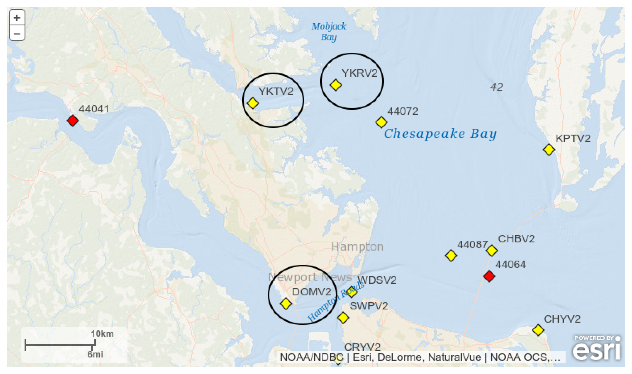
All experiments presented in this work were conducted based on data from three meteorological stations located on the coast of the state of Virginia (USA): YKTV2, YKRV2 and DOMV2. Data for these and many other stations is freely available from the United States National Data Buoy Center [20]. The location of the selected stations is shown in Figure 2.
In a previous work [15] the correlation between the meteorological data of the different stations was analysed and the data series of station YKTV2 was reconstructed from one and two of the remaining stations, using different metrics in addition to the classical metric proposed by Monache [3] to find the analogues. It was then found that the weather at stations DOMV2 and YKRV2 followed a similar pattern although, due to their different locations, certain meteorological values differ.
However, since the alternative metrics look for a similar evolution of the weather during the time window and not for similar values as the classical metric, both stations are suitable for data reconstruction at station YKTV2. Therefore, these three stations were also used for the same purpose in this paper. Table 1 contains their coordinates and roles.
The data used in this study range from 2011 to 2019 and includes six different meteorological variables: Pressure (PRES), Air Temperature (ATMP), Mean Wind Speed (WSPD) and Gust Speed (GST). PRES is the pressure [hPa] measured at sea level, ATMP is the air temperature [°C], WSPD is the wind speed [m/s] averaged over an 8 min period for buoys and a 2 min period for land stations, and GST is the peak gust speed of 5 or 8 s gust speed [m/s] measured during the 8 min or 2 min period (for details see [20]). The time-series records are based on samples taken every 6 min (). The time-series are not always complete. Data are missing for periods that can be short (hours) or long (months)—Table 2 shows the availability of data over the period studied.
Table 2 contains basic statistics of the relevant variables for each station, such as the minimum (Min), average (Mean) and maximum (Max) values, along with the number of missing records (# NA) and the percentage of available records (Availability) in the time-series. We verified that the amount of missing data did not exceed 3.3%. If the missing records did not exceed the size of the subsets , they were filled by interpolation from nearby values. If the range was longer, the corresponding records were ignored.
The 9 years of data was divided into two groups: (i) data for a training period, from the beginning of 2011 to the end of 2017; (ii) data for a prediction period, from the beginning of 2018 to the end of 2019. In the prediction period, data for station was hindcast from data of the stations and , hence acting as predictor datasets.
Having data for a period of 9 years with a time-step implied a large number of data set vectors, which caused a considerable computational effort when applying the classical AnEn method. Therefore, the predictions in the forecast period were limited to the interval between 10 am and noon, based on the same intervals in the historical dataset. Theoretically, 10 samples per hour, 2 h per day, for 7 historical years would correspond to a total number of 51,100 samples and, accordingly, to the same number of possible analogue vectors (each centred in one of these samples); in the end, only a total of 43,238 records were used due to some missing data.
4.2. Prediction Error Metrics
As real data was available for the predicted period, it was possible to compare the predictions () with the observed values (). Following Chai and Draxler [21] recommendations, multiple metrics were used to assess the model accuracy, starting with the Bias,
where is the number of predictions, is a prediction, and is the corresponding truth value. The Bias measures the average error compared to the truth, however, allowing over- and under-predictions to cancel out. This metric can be interpreted as a rough approximation of the systematic error in the prediction. Thus, complementary to the Bias, the Root Mean-Squared Error (RMSE) is also used:
The RMSE is useful because the squared terms give a higher weight to higher errors. Thus, the RMSE will be higher if the model makes predictions which are far from the truth, even if these erroneous predictions are few in number.
The Standard Deviation of the Error (SDE) is computed from the Bias and RMSE metrics, corresponding to:
The SDE represents the error due to variance; hence, it can be used as a rough approximation of the random error in the prediction.
Another metric, akin to the RMSE, is the Mean Absolute Error (MAE), being recommended by Chai and Draxler [21] as a complement to the former. The MAE is defined as
thus, computing the average distance to the truth in absolute values. This is different from the Bias as the errors do not cancel out, whilst yielding a value smoother than the RMSE.
A low Bias and a high MAE indicates that the model is not really accurate but that its predictions are sometimes higher and sometimes lower than the truth. Thus, considering the MAE is necessary to really understand how the error in the prediction is distributed, as it also shows the systematic error but this time in terms of the absolute distance.
In addition to these individual metrics, this paper also uses a combined error metric (CE): , which is the sum of the absolute values of the individual error metrics (note that only Bias can be negative). When evaluating the impact of different values of critical parameters on the methods under study, the combined metric is a heuristic that allows the most favourable (in terms of error) parameter values to be easily identified: these values are those that lead to the absolute minimum of CE.
However, since many of the values of CE registered in the experiments are close to each other, a small tolerance of up to is allowed; this means that values of CE within an excess of up to from the absolute minimum are considered statistically identical, leading to several equivalent choices for the parameters of the methods under investigation.
5. Experimental Evaluation
In this section, the K-means AnEn method is evaluated and compared with the classical AnEn approach, in the context of a hindcasting problem with the previously presented meteorological dataset. All results were produced by implementations of both AnEn approaches in R [22]. For the K-means variant, the built-in function kmeans was used.
5.1. Variation of the Number of Clusters
The evaluation starts by analysing the impact of the variation of the number of clusters formed () in the prediction errors. This number, and the amount of clusters effectively used (, with ), are fundamental parameters of the cluster-based approach to the AnEn method investigated in this work: the number of clusters formed has an influence on the number of subsets (vectors) in each cluster (fewer clusters will have more subsets, and vice versa); correspondingly, this determines the number of observations used to derive the predictions and, ultimately, that number will affect the predictions accuracy.
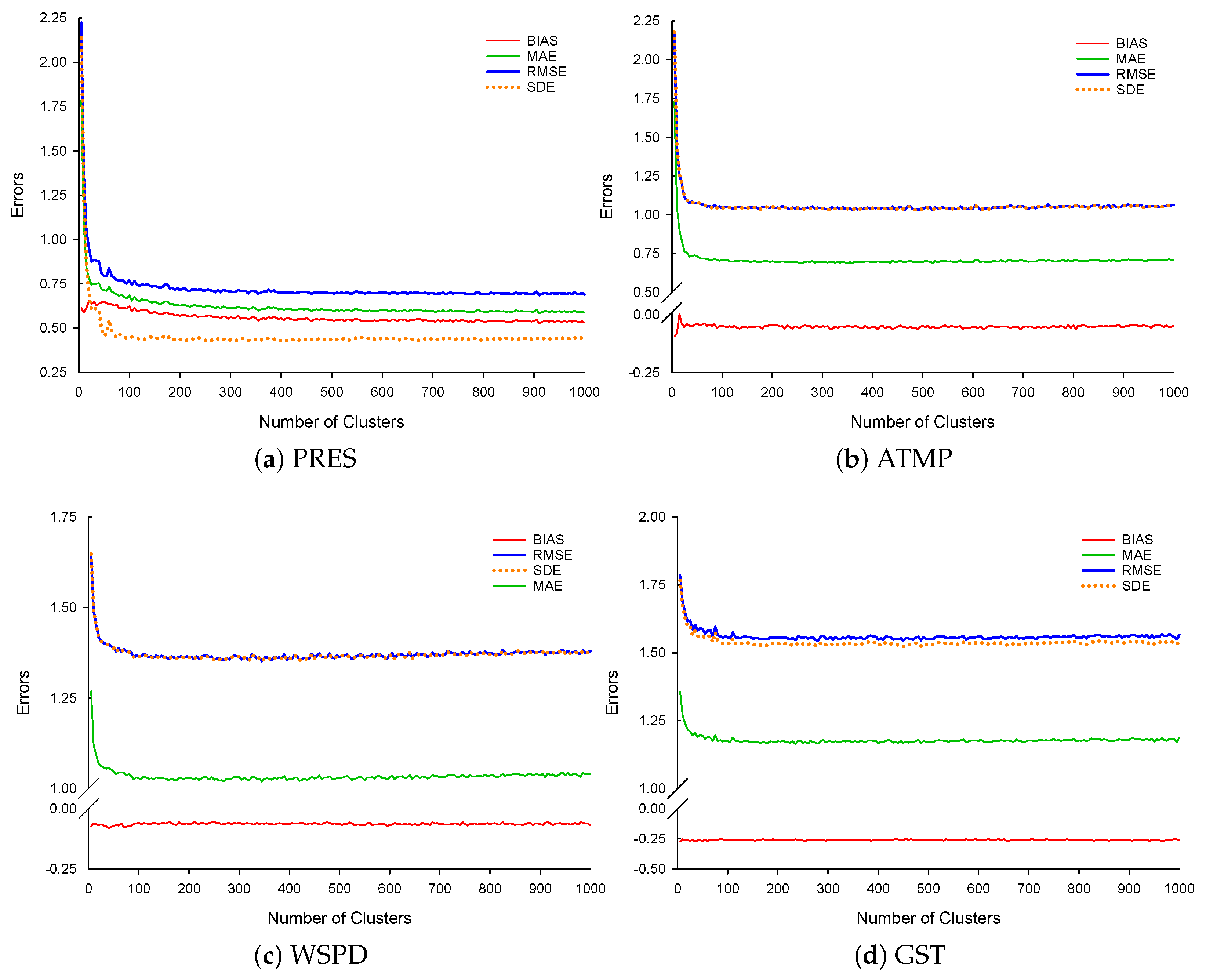
The assessed scenario concerns the dependent stations variant, where a single cluster () is selected in each predictor station to generate the forecast. The results, shown in Figure 3, were obtained with ; thus, for each meteorological variable there were m= = 43,228 subsets (vectors) in each predictor dataset from which clusters could be formed and each subset consisted of 11 values (covering a time frame of 66 min).
In Figure 3, a similarity in the behaviour of the errors with the variation of for the variables ATMP, GST and WSPD can be seen: the errors first decrease significantly with the increase of up to ; then they decrease moderately up to and stabilize thereafter. The variable PRES shows a different behaviour: the errors continue to decrease with the increasing of . This is possibly due to the fact that the variable PRES does not show large fluctuations over a short period of time, and therefore the smaller clusters describe its behaviour best due to the lower variance.
Determining the optimal value of a priori is difficult because each variable has different behaviour. Setting bellow 100 may result in a high error for each variable. For the variables ATMP, GST and WSPD, there is a small tendency for errors to increase as the value of increases, which would justify rejecting large values for . However, this is not true for the variable PRES, as the errors are inversely proportional to the value.
A possible heuristic to define a single common value is to set it as the square root of the total number of records in the training period () [16]. Considering the datasets used in this work, it would follow that . Another approach is to define it as the average of the values that ensure the lowest prediction errors for the different variables. In this case, the variable PRES is left aside (due to its singular behaviour) and, based on the values shown in Figure 3 for the other three variables, a “universal” value for would be ≈350; although this is not an optimal value for the variable PRES, it is a good compromise, since the error for this variable decreases only slightly after .
5.2. Variation of the Number of Analogues
Having determined the number of clusters to be formed () and effectively used (), there is still the possibility of refining the prediction by limiting the number of analogues (i.e., the number of subsets or vectors) provided by each selected cluster. Thus, it is possible to use all the subsets contained in a selected cluster or, alternatively, a smaller set ordered by affinity to the centroid of that cluster.
The effects of varying on forecast errors can be seen in Table 3 for the reconstruction of the four meteorological variables studied. These results were obtained keeping some parameters of the evaluation of the previous section (dependent stations, , ) but now with a limitation of the number of clusters formed to (according to the heuristic defined in the same section). In the table, the rows with the smallest verified errors for each of the meteorological variables are highlighted in bold. Moreover, the special value “∞” for means that all analogue candidates (all subsets/vectors) of a cluster were used.
The results in Table 3 show that, with the exception of the pressure variable (PRES), the lowest error values were obtained at high values. However, the differences between the smallest errors and those obtained with all subsets of the cluster were very small. This result indicates that for the variables ATMP, WSPD and GST the whole cluster can be used as an analogue ensemble. In contrast, for the variable PRES a low value is preferable.
5.3. Variation of the Analogue Size
The parameter k is used to define the number of records that constitute an analogue vector: that number is , with consecutive records in time separated by a time-step. Therefore, k also corresponds to half of the total number of time-steps within an analogue vector, and so k may also be referred to as the “half (time-)window size”.
All experiments discussed so far were conducted with (analogue size = 11). In this section, the effects of varying k on the prediction errors are evaluated, while still considering the dependent stations scenario. Consistent with the results of the previous sections, the other relevant parameters were , , = all cluster analogues.
Table 4 contains the results of varying the analogue size by varying k. The lowest errors (in bold) were obtained with a different set of k values for each variable. However, it is worth noting that was shared by all variables and is therefore a good default value. This corresponds to a vector time span of 60 min between the first and the last sample. Therefore, one hour appears to be a reasonable time window to assess the correlation between the analogue candidates and the predictor and then make accurate predictions.
Another observation deserves an explanation: for , the errors in Table 4 do not match the corresponding errors () in Table 3, although they were generated with the same parameters. This is because the values in these tables come from different runs of the K-means-based method, which is inherently non-deterministic, resulting in differences in the clusters formed in each run, which translates into differences in the errors produced.
5.4. Dependent vs. Independent Stations
Thus far, all results presented were obtained using the dependent station approach (Algorithm 4). In this section, a comparison is made with the results of Algorithm 3, which implements an independent-stations approach. All results refer to the same parameters: , , and (all analogue candidates of the cluster used).
In Table 5, the best errors for each situation are shown in bold. For the independent approach, there is only one error of each type for each variable. For the dependent approach, two errors are given: the first is from row of Table 3; the second (marked *) is from Table 4 and corresponds to the worst of the best values within the range of given in Section 4.2. This is to show that even the worst of the best errors measured with the dependent approach are generally (with very few exceptions) smaller than the errors obtained with the independent approach.
From the results in Table 5—and in particular from the column of the combined error (CE)—it can be concluded that the use of the dependent method leads to a reduction of the prediction errors, even if this reduction was not very significant in some cases.
5.5. Prediction with Variables Different from the Predicted
In the previous sections, the data of the predictor stations corresponded to the data of the predicted variable in all predictions. For example, if the variable was ATMP, only the data from that variable were used to select the analogues. However, in a scenario where the stations used as predictors do not have historical records of the variable being predicted, the only alternative is to make predictions with a different variable, and the impact of this approach will vary depending on the correlation between the variables at stake.
Table 6 shows the prediction errors for each meteorological variable as a function of different predictor variables, keeping the same general parameters used so far: dependent approach, , , and (all clusters analogue candidates used).
As can be seen in Table 6, the results for the variables PRES and ATMP are worse when a predictor variable other than the predicted one is used. However, for the WSPD and GST variables, the results obtained when one is used to predict the other are very similar to those for self-prediction, hinting that these two variables are highly correlated. These results suggest that the best analogues are obtained when predictors that are well correlated with the predicted variable are used.
6. Computational Performance
The classical AnEn method compares the predictor value with all historical values of the training period (step 1 of Figure 1) using the metrics of the Formulas (2) or (5). As discussed in Section 3.1, this requires a considerable amount of computation, especially if done purely sequentially. Furthermore, although it is possible to parallelize the analogues search [12], the longer the prediction period, the greater this effort will be.
A major advantage of determining analogues via K-means clustering is the potential for a dramatic reduction in overall computational time. As explained in Section 3.2, this reduction stems from the fact that clustering (which, since it is only done once, is still the most time-consuming phase in this approach), followed by the comparison of each cluster centroid with the predictor, is much faster than going through all possible analogues of the historical dataset and comparing them with the predictor.
This section describes the computational performance of implementations in R [22] of the classical and K-means-based AnEn methods that were specifically coded for this research. These implementations took advantage of built-in facilities in R for parallel execution, namely the parSapply function. Execution took place in a multicore environment provided by a Linux installation in a computer with two 16-core AMD EPYC 7351 CPUs (32 cores/64 threads in total) and 256 GB RAM.
For this performance study, the values chosen for the critical parameters of both AnEn methods were those previously shown to produce the lowest prediction errors. For the classical AnEN variant, these correspond to and (recommended parameters in the paper [16]), while for the K-means variant, they correspond to those established in this paper (dependent approach, , , and ).
The performance results are presented in Table 7 and Table 8. They unfold for the prediction of different variables, with different AnEn methods and a different number of CPU threads.
Table 7 allows a comparison of the best errors, total prediction times and the Speedup of the K-means variant against the classic method. The errors shown are limited to the Bias and SDE, which represent the systematic and random error, respectively. The results show that the K-means variant generally leads to more accurate predictions. Only for the variable PRES is this not the case, and even there the error differences are small. This is related to the discussion in Section 5.1 and Section 5.2, namely that the variable PRES requires a higher number of clusters due to its lack of variance for short time scales, so that each cluster characterizes a smaller sample, or alternatively, the number of subsets () used as analogues in the cluster must be small.
With regard to the prediction times, these are similar for different variables when using the same AnEn variant. However, between the two AnEn variants, the prediction times are quite different and are up to two orders of magnitude apart, with the K-means variant being considerably faster (from 15- to 22-times faster) than the classical variant when using sequential processing (), and keeping a lead when using parallel processing (although the K-means Speedup decreases with the number of CPU threads used).
In fact, the classical variant benefits greatly from the increase in the number of CPU threads used, since the computation of the similarity metric for each analogue candidate (step 1 in Figure 1) is independent of any other candidate and is thus performed in parallel. On the other hand, the K-means version does not benefit as much from the increased number of CPU threads, since only the similarity of centroids to the predictor can be computed in parallel, and their number is much smaller than the number of analogue candidates in the classical version.
Table 8 provides measures of the computational Speedup () and Efficiency () as a function of the number (n) of CPU threads used. It can be observed that the classical approach has a higher Speedup and Efficiency for each . Compared to the K-means approach, the classical approach has a Speedup that increases as n increases, and the loss of Efficiency is lower. As mentioned earlier, this method benefits greatly from the parallelization of analogue selection. However, to compete with the K-means variant in terms of prediction time, it needs a high number of CPU threads (as can be seen in Table 7, the K-means variant is still faster even with 64 CPU threads).
The results presented in this section show that the clustering-based variant of the AnEn method has better computational efficiency compared with the original version proposed by Monache [3,4]. Moreover, it is a reliable alternative that allows the reconstruction of missing data with errors smaller than or equal to the ones of the classical version.
7. Conclusions
The K-means AnEn variant is a worthy alternative to the classical AnEn method, with the same or better accuracy and much higher performance. This new variant facilitates using larger data sets and consequently solving larger problems in the various application domains of the AnEn method, such as hindcasting, forecasting and downscaling.
The numerical efficiency of this new AnEn variant depends on some of its most important parameters, namely the number of clusters to be formed (), the number of clusters effectively used (), the number of analogues () to be considered in each of the selected clusters and the time span (k) of each analog.
The way in which the data from multiple predictor stations are used to select the analogues (independently or with time dependence) and the use of the same or correlated predictor variables to make the predictions also have a measurable impact on their accuracy.
The experimental results showed that, for most of the meteorological variables considered, must be large enough for the subsets (vectors) included in each cluster to be sufficiently analogous to each other. Furthermore, it was shown that the use of a single best cluster () and all the subsets contained in it as analogues, together with an analogue time span of one hour (), provided optimal or near-optimal accuracy.
As expected, the use of the same or highly correlated variables proved crucial to achieve the desired accuracy and the use of a dependent-stations approach proved beneficial (albeit slightly) for the same purpose.
Finally, from a computational-performance standpoint, the K-means-based AnEn approach has an undeniable advantage over the classical AnEn method: the prediction times of the former are much lower (up to two orders of magnitude) than those of the latter. However, the K-means variant doesn’t benefit from parallelization as much as the classical one. As the number of CPU threads used increases, the latter becomes more competitive: its Speedup scales better than that of the K-means variant, and the efficiency remains higher.
In the future, we want to investigate whether the application of machine-learning techniques brings advantages over the K-means-based variant proposed in this work.
Author Contributions
Conceptualization, C.B. and C.V.R.; methodology, C.B. and J.R.; software, J.R. and L.A.; validation, L.A., J.R. and C.V.R.; formal analysis, C.B. and C.V.R.; investigation, C.B. and L.A.; resources, J.R.; data curation, L.A. and C.V.R.; writing—original draft preparation, C.B.; writing—review and editing, J.R.; visualization, C.V.R.; supervision, C.B. and J.R.; project administration, C.B. and J.R.; funding acquisition, C.B. and J.R. All authors have read and agreed to the published version of the manuscript.
Funding
This work has been partially supported by FCT—Fundação para a Ciência e Tecnologia within the Project Scope: UIDB/05757/2020.
Institutional Review Board Statement
Not applicable.
Informed Consent Statement
Not applicable.
Data Availability Statement
The data used in this study are freely available from the United States National Data Buoy Center at https://www.ndbc.noaa.gov (accessed on 28 April 2022).
Conflicts of Interest
The authors declare no conflict of interest.
References
- Lorenz, E.N. Atmospheric Predictability as Revealed by Naturally Occurring Analogues. J. Atmos. Sci. 1969, 26, 636–646. [Google Scholar] [CrossRef] [Green Version]
- Dool, H.M.V.D. A New Look at Weather Forecasting through Analogues. Mon. Weather Rev. 1989, 117, 2230–2247. [Google Scholar] [CrossRef] [Green Version]
- Monache, L.D.; Nipen, T.; Liu, Y.; Roux, G.; Stull, R. Kalman Filter and Analog Schemes to Postprocess Numerical Weather Predictions. Mon. Weather Rev. 2011, 139, 3554–3570. [Google Scholar] [CrossRef] [Green Version]
- Monache, L.D.; Eckel, F.A.; Rife, D.L.; Nagarajan, B.; Searight, K. Probabilistic Weather Prediction with an Analog Ensemble. Mon. Weather Rev. 2013, 141, 3498–3516. [Google Scholar] [CrossRef] [Green Version]
- Alessandrini, S.; Monache, L.D.; Sperati, S.; Nissen, J.N. A novel application of an analog ensemble for short-term wind power forecasting. Renew. Energy 2015, 76, 768–781. [Google Scholar] [CrossRef]
- Alessandrini, S.; Monache, L.D.; Sperati, S.; Cervone, G. An analog ensemble for short-term probabilistic solar power forecast. Appl. Energy 2015, 157, 95–110. [Google Scholar] [CrossRef] [Green Version]
- Cervone, G.; Clemente-Harding, L.; Alessandrini, S.; Delle Monache, L. Short-term photovoltaic power forecasting using Artificial Neural Networks and an Analog Ensemble. Renew. Energy 2017, 108, 274–286. [Google Scholar] [CrossRef] [Green Version]
- Rozoff, C.M.; Alessandrini, S. A Comparison between Analog Ensemble and Convolutional Neural Network Empirical-Statistical Downscaling Techniques for Reconstructing High-Resolution Near-Surface Wind. Energies 2022, 15, 1718. [Google Scholar] [CrossRef]
- Solomou, E.; Pappa, A.; Kioutsioukis, I.; Poupkou, A.; Liora, N.; Kontos, S.; Giannaros, C.; Melas, D. Analog ensemble technique to post-process WRF-CAMx ozone and particulate matter forecasts. Atmos. Environ. 2021, 256, 118439. [Google Scholar] [CrossRef]
- Yang, D.; van der Meer, D. Post-processing in solar forecasting: Ten overarching thinking tools. Renew. Sustain. Energy Rev. 2021, 140, 110735. [Google Scholar] [CrossRef]
- Vannitsem, S.; Bremnes, J.B.; Demaeyer, J.; Evans, G.R.; Flowerdew, J.; Hemri, S.; Lerch, S.; Roberts, N.; Theis, S.; Atencia, A.; et al. Statistical Postprocessing for Weather Forecasts: Review, Challenges, and Avenues in a Big Data World. Bull. Am. Meteorol. Soc. 2021, 102, E681–E699. [Google Scholar] [CrossRef]
- Hu, W.; Vento, D.; Su, S. Parallel Analog Ensemble—The Power of Weather Analogs. In Proceedings of the 2020 Improving Scientific Software Conference, Turin, Italy, 25–27 November 2020; pp. 1–14. [Google Scholar] [CrossRef]
- Hu, W.; Cervone, G.; Merzky, A.; Turilli, M.; Jha, S. A new hourly dataset for photovoltaic energy production for the continental USA. Data Brief 2022, 40, 107824. [Google Scholar] [CrossRef] [PubMed]
- Balsa, C.; Rodrigues, C.V.; Araújo, L.; Rufino, J. Hindcasting with Cluster-Based Analogues. In Communications in Computer and Information Science; Springer International Publishing: Berlin/Heidelberg, Germany, 2021; pp. 346–360. [Google Scholar] [CrossRef]
- Balsa, C.; Rodrigues, C.V.; Lopes, I.; Rufino, J. Using Analog Ensembles with Alternative Metrics for Hindcasting with Multistations. ParadigmPlus 2020, 1, 1–17. [Google Scholar] [CrossRef]
- Araújo, L.; Balsa, C.; Rodrigues, C.V.; Rufino, J. Parametric Study of the Analog Ensembles Algorithm with Clustering Methods for Hindcasting with Multistations. In Advances in Intelligent Systems and Computing; Springer International Publishing: Berlin/Heidelberg, Germany, 2021; pp. 544–559. [Google Scholar] [CrossRef]
- Chesneau, A.; Balsa, C.; Rodrigues, C.V.; Lopes, I.M. Hindcasting with multistations using analog ensembles. In Proceedings of the CEUR Workshop Proceedings (CEUR-WS), Copenhagen, Denmark, 30 March 2019; Volume 2486, pp. 215–229. [Google Scholar]
- Eldén, L. Matrix Methods in Data Mining and Pattern Recognition; SIAM: Philadelphia, PA, USA, 2007. [Google Scholar]
- Garey, M.R.; Johnson, D.S. Computers and Intractability—A Guide to the Theory of NP-Completeness; W. H. Freeman & Co.: New York, NY, USA, 1990. [Google Scholar]
- National Data Buoy Center. Available online: https://www.ndbc.noaa.gov/ (accessed on 15 April 2022).
- Chai, T.; Draxler, R.R. Root mean square error (RMSE) or mean absolute error (MAE)?—Arguments against avoiding RMSE in the literature. Geosci. Model Dev. 2014, 7, 1247–1250. [Google Scholar] [CrossRef] [Green Version]
- R Core Team. R: A Language and Environment for Statistical Computing; R Foundation for Statistical Computing: Vienna, Austria, 2017. [Google Scholar]
Figure 1.
Reconstruction of meteorological data with the analogues ensemble method ().

Figure 2.
Geolocation of the NDBC meteorological stations in Virginia (USA) [20].
Figure 2.
Geolocation of the NDBC meteorological stations in Virginia (USA) [20].

Figure 3.
Prediction errors as a function of the number of clusters ().


Table 1.
Meteorological stations.
| Station | Code | Location | Role |
|---|---|---|---|
| YKTV2 | 37°1336 N 76°2843 W | Predicted | |
| YKRV2 | 37°155 N 76°2033 W | Predictor | |
| DOMV2 | 36°5744 N 76°2527 W | Predictor |
Table 2.
Data availability in the meteorological stations.
| Variable | Min | Mean | Max | # NA | Availability |
|---|---|---|---|---|---|
| Station —YKTV2 | |||||
| PRES [hPa] | 974.70 | 1017.34 | 1044.30 | 20,157 | 97.44% |
| ATMP [°C] | −13.50 | 16.06 | 37.80 | 26,102 | 96.69% |
| WSPD [m/s] | 0.00 | 4.26 | 23.80 | 25,127 | 96.81% |
| GST [m/s] | 0.00 | 5.44 | 32.80 | 25,156 | 96.81% |
| Station —YKRV2 | |||||
| PRES [hPa] | 972.60 | 1017.35 | 1043.90 | 18,785 | 97.62% |
| ATMP [°C] | −12.80 | 15.86 | 36.30 | 22,566 | 97.14% |
| WSPD [m/s] | 0.00 | 5.93 | 27.60 | 24,795 | 96.86% |
| GST [m/s] | 0.00 | 6.88 | 39.60 | 24,910 | 96.84% |
| Station —DOMV2 | |||||
| PRES [hPa] | 972.80 | 1017.77 | 1044.50 | 19,992 | 97.47% |
| ATMP [°C] | −12.60 | 16.13 | 37.20 | 25,194 | 96.81% |
| WSPD [m/s] | 0.00 | 3.91 | 24.30 | 25,866 | 96.72% |
| GST [m/s] | 0.00 | 5.28 | 32.10 | 25,897 | 96.72% |
Table 3.
Prediction errors as a function of the number of analogues ().
| Bias | RMSE | MAE | SDE | CE | Bias | RMSE | MAE | SDE | CE | |
|---|---|---|---|---|---|---|---|---|---|---|
| PRES | ATMP | |||||||||
| 50 | 0.528 | 0.679 | 0.580 | 0.427 | 2.214 | −0.056 | 1.049 | 0.703 | 1.047 | 2.855 |
| 100 | 0.562 | 0.702 | 0.613 | 0.420 | 2.297 | −0.055 | 1.048 | 0.696 | 1.046 | 2.845 |
| 150 | 0.559 | 0.703 | 0.614 | 0.427 | 2.303 | −0.058 | 1.047 | 0.696 | 1.045 | 2.846 |
| 200 | 0.561 | 0.711 | 0.617 | 0.436 | 2.325 | −0.049 | 1.030 | 0.691 | 1.029 | 2.799 |
| 250 | 0.555 | 0.706 | 0.612 | 0.436 | 2.309 | −0.060 | 1.048 | 0.696 | 1.046 | 2.850 |
| 300 | 0.557 | 0.710 | 0.614 | 0.440 | 2.321 | −0.052 | 1.027 | 0.691 | 1.026 | 2.796 |
| 350 | 0.553 | 0.705 | 0.610 | 0.436 | 2.304 | −0.050 | 1.030 | 0.688 | 1.028 | 2.796 |
| 400 | 0.565 | 0.706 | 0.618 | 0.423 | 2.312 | −0.053 | 1.041 | 0.697 | 1.040 | 2.831 |
| ∞ | 0.561 | 0.712 | 0.618 | 0.439 | 2.330 | −0.037 | 1.040 | 0.695 | 1.039 | 2.811 |
| WSPD | GST | |||||||||
| 50 | −0.121 | 1.377 | 1.032 | 1.372 | 3.902 | −0.341 | 1.579 | 1.191 | 1.542 | 4.653 |
| 100 | −0.097 | 1.366 | 1.025 | 1.362 | 3.850 | −0.317 | 1.564 | 1.179 | 1.532 | 4.592 |
| 150 | −0.075 | 1.362 | 1.026 | 1.360 | 3.823 | −0.284 | 1.571 | 1.184 | 1.545 | 4.584 |
| 200 | −0.067 | 1.357 | 1.024 | 1.355 | 3.803 | −0.269 | 1.563 | 1.178 | 1.539 | 4.549 |
| 250 | −0.068 | 1.365 | 1.027 | 1.364 | 3.824 | −0.260 | 1.554 | 1.174 | 1.532 | 4.520 |
| 300 | −0.060 | 1.352 | 1.019 | 1.351 | 3.782 | −0.257 | 1.561 | 1.176 | 1.540 | 4.534 |
| 350 | −0.060 | 1.358 | 1.024 | 1.357 | 3.799 | −0.261 | 1.557 | 1.172 | 1.535 | 4.525 |
| 400 | −0.057 | 1.364 | 1.028 | 1.362 | 3.811 | −0.260 | 1.553 | 1.175 | 1.531 | 4.519 |
| ∞ | −0.059 | 1.355 | 1.024 | 1.354 | 3.792 | −0.263 | 1.559 | 1.172 | 1.537 | 4.531 |
Table 4.
Prediction errors as a function of the half time-window size (k).
| k | Bias | RMSE | MAE | SDE | CE | Bias | RMSE | MAE | SDE | CE |
|---|---|---|---|---|---|---|---|---|---|---|
| PRES | ATMP | |||||||||
| 1 | 0.574 | 0.717 | 0.628 | 0.430 | 2.349 | −0.067 | 1.043 | 0.690 | 1.041 | 2.841 |
| 2 | 0.571 | 0.712 | 0.622 | 0.425 | 2.330 | −0.060 | 1.038 | 0.690 | 1.036 | 2.824 |
| 3 | 0.557 | 0.704 | 0.612 | 0.430 | 2.303 | −0.059 | 1.046 | 0.697 | 1.044 | 2.846 |
| 4 | 0.570 | 0.713 | 0.623 | 0.428 | 2.334 | −0.058 | 1.049 | 0.699 | 1.047 | 2.853 |
| 5 | 0.550 * | 0.703 * | 0.607 * | 0.438 * | 2.298 * | −0.053 * | 1.031 * | 0.685 * | 1.029 * | 2.798 * |
| 6 | 0.554 | 0.708 | 0.610 | 0.441 | 2.313 | −0.049 | 1.039 | 0.693 | 1.038 | 2.819 |
| 7 | 0.548 | 0.701 | 0.605 | 0.437 | 2.291 | −0.047 | 1.048 | 0.699 | 1.047 | 2.841 |
| 8 | 0.549 | 0.705 | 0.608 | 0.442 | 2.304 | −0.043 | 1.045 | 0.700 | 1.044 | 2.832 |
| 9 | 0.554 | 0.708 | 0.612 | 0.441 | 2.315 | −0.034 | 1.044 | 0.705 | 1.043 | 2.826 |
| 10 | 0.557 | 0.713 | 0.618 | 0.445 | 2.333 | −0.040 | 1.042 | 0.699 | 1.041 | 2.822 |
| WSPD | GST | |||||||||
| 1 | −0.063 | 1.364 | 1.028 | 1.362 | 3.817 | −0.258 | 1.556 | 1.172 | 1.535 | 4.521 |
| 2 | −0.060 | 1.366 | 1.029 | 1.365 | 3.820 | −0.258 | 1.558 * | 1.169 | 1.537 * | 4.522 |
| 3 | −0.060 | 1.359 | 1.026 | 1.357 | 3.802 * | −0.257 | 1.557 | 1.172 | 1.536 | 4.522 |
| 4 | −0.062 | 1.365 | 1.029 | 1.364 | 3.820 | −0.256 | 1.558 * | 1.176 * | 1.537 * | 4.527 * |
| 5 | −0.055 | 1.361 * | 1.027 * | 1.359 * | 3.802 * | −0.261 * | 1.556 | 1.171 | 1.534 | 4.522 |
| 6 | −0.064 * | 1.357 | 1.025 | 1.356 | 3.802 * | −0.258 | 1.557 | 1.171 | 1.536 | 4.522 |
| 7 | −0.061 | 1.357 | 1.027 * | 1.355 | 3.800 | −0.266 | 1.566 | 1.180 | 1.543 | 4.555 |
| 8 | −0.066 | 1.368 | 1.032 | 1.367 | 3.833 | −0.258 | 1.568 | 1.186 | 1.546 | 4.558 |
| 9 | −0.062 | 1.364 | 1.030 | 1.363 | 3.819 | −0.251 | 1.562 | 1.180 | 1.542 | 4.535 |
| 10 | −0.071 | 1.379 | 1.038 | 1.377 | 3.865 | −0.257 | 1.561 | 1.176 | 1.539 | 4.533 |
Table 5.
Prediction errors with dependent and independent stations.
| Variable | Dependency | Bias | RMSE | MAE | SDE | CE |
|---|---|---|---|---|---|---|
| PRES | Yes | 0.561, 0.550 * | 0.712, 0.703 * | 0.618, 0.607 * | 0.439, 0.438 * | 2.330, 2.298 * |
| No | 0.653 | 0.732 | 0.685 | 0.332 | 2.402 | |
| ATMP | Yes | −0.037, −0.053 * | 1.040, 1.031 * | 0.695, 0.685 * | 1.039, 1.029 * | 2.811, 2.798 * |
| No | −0.051 | 1.047 | 0.685 | 1.045 | 2.828 | |
| WSPD | Yes | −0.059, −0.064 * | 1.355, 1361 * | 1.024, 1.027 * | 1.354, 1.359 * | 3.792, 3.811 * |
| No | −0.086 | 1.558 | 1.193 | 1.555 | 4.392 | |
| GST | Yes | −0.263, −0.261 * | 1.559, 1.558 * | 1.172, 1.176 * | 1.537, 1.537 * | 4.531, 4.532 * |
| No | −0.278 | 1.681 | 1.290 | 1.658 | 4.907 |
Table 6.
Prediction errors for different variables used as predictors.
| Predicted | Predictor | Bias | RMSE | MAE | SDE | CE |
|---|---|---|---|---|---|---|
| PRES | PRES | 0.564 | 0.713 | 0.619 | 0.435 | 2.331 |
| ATMP | −0.642 | 6.651 | 5.216 | 6.620 | 19.129 | |
| WSPD | −0.210 | 6.518 | 5.085 | 6.515 | 18.328 | |
| GST | −0.162 | 6.590 | 5.169 | 6.588 | 18.509 | |
| ATMP | PRES | 0.343 | 7.998 | 6.621 | 7.991 | 22.953 |
| ATMP | −0.050 | 1.038 | 0.693 | 1.037 | 2.818 | |
| WSPD | −0.558 | 8.771 | 7.670 | 8.754 | 25.753 | |
| GST | −0.519 | 8.916 | 7.802 | 8.901 | 26.138 | |
| WSPD | PRES | 0.222 | 2.587 | 2.067 | 2.577 | 7.453 |
| ATMP | −0.015 | 2.443 | 1.901 | 2.443 | 6.802 | |
| WSPD | −0.059 | 1.359 | 1.024 | 1.358 | 3.800 | |
| GST | −0.070 | 1.327 | 1.005 | 1.325 | 3.727 | |
| GST | PRES | 0.012 | 3.196 | 2.549 | 3.196 | 8.953 |
| ATMP | −0.198 | 3.073 | 2.402 | 3.067 | 8.740 | |
| WSPD | −0.261 | 1.609 | 1.203 | 1.588 | 4.661 | |
| GST | −0.257 | 1.554 | 1.171 | 1.533 | 4.515 |
Table 7.
Classical vs. K-means AnEn: prediction errors, computation times [s] and K-means Speedup.
| Errors | Number of CPU Threads (n) and Prediction Times () | |||||||||
|---|---|---|---|---|---|---|---|---|---|---|
| Variable | AnEn | Bias | SDE | 1 | 2 | 4 | 8 | 16 | 32 | 64 |
| PRES | Classic | 0.278 | 0.412 | 206.0 | 107.0 | 73.0 | 41.0 | 22.6 | 16.9 | 14.4 |
| K-means | 0.550 | 0.438 | 9.0 | 6.0 | 5.0 | 4.0 | 3.7 | 3.4 | 3.7 | |
| Speedup | – | – | 22.89 | 17.83 | 14.6 | 10.25 | 6.11 | 4.97 | 3.89 | |
| ATMP | Classic | 0.000 | 1.070 | 205.0 | 111.0 | 52.0 | 39.0 | 21.2 | 17.0 | 15.1 |
| K-means | −0.037 | 1.029 | 9.0 | 6.0 | 5.0 | 4.2 | 3.4 | 3.3 | 3.7 | |
| Speedup | – | – | 22.78 | 18.5 | 10.4 | 9.29 | 6.24 | 5.15 | 4.08 | |
| WSPD | Classic | −0.206 | 2.064 | 186.0 | 98.0 | 50.0 | 27.0 | 15.3 | 10.4 | 9.5 |
| K-means | −0.059 | 1.354 | 12.0 | 10.0 | 7.1 | 6.6 | 6.3 | 6.5 | 6.8 | |
| Speedup | – | – | 15.5 | 9.8 | 7.04 | 4.09 | 2.43 | 1.6 | 1.4 | |
| GST | Classic | −0.530 | 2.132 | 200.0 | 98.0 | 53.0 | 27.0 | 15.3 | 10.9 | 8.3 |
| K-means | −0.261 | 1.537 | 13.0 | 11.0 | 8.0 | 6.6 | 6.7 | 6.1 | 6.7 | |
| Speedup | – | – | 15.38 | 8.91 | 6.63 | 4.09 | 2.28 | 1.79 | 1.24 | |
Table 8.
Classical AnEn vs. K-means AnEn: Speedup and Efficiency (%).
| Number of CPU Threads (n), Speedup () and Efficiency () | |||||||||
|---|---|---|---|---|---|---|---|---|---|
| Variable | AnEn | Measure | 1 | 2 | 4 | 8 | 16 | 32 | 64 |
| PRES | Classic | 1.00 | 1.92 | 2.84 | 4.98 | 9.12 | 12.20 | 14.32 | |
| (%) | 100.0 | 96.2 | 71.0 | 62.3 | 57.0 | 38.1 | 22.4 | ||
| K-means | 1.00 | 1.47 | 1.91 | 2.15 | 2.38 | 2.59 | 2.38 | ||
| (%) | 100.0 | 73.3 | 47.8 | 26.8 | 14.9 | 8.1 | 3.7 | ||
| ATMP | Classic | 1.00 | 1.85 | 3.94 | 5.27 | 9.67 | 12.06 | 13.58 | |
| (%) | 100.0 | 92.7 | 98.4 | 65.9 | 60.5 | 37.7 | 21.2 | ||
| K-means | 1.00 | 1.51 | 1.93 | 2.12 | 2.62 | 2.70 | 2.41 | ||
| (%) | 100.0 | 75.4 | 48.4 | 26.5 | 16.4 | 8.4 | 3.8 | ||
| WSPD | Classic | 1.00 | 1.91 | 3.70 | 6.93 | 12.18 | 17.92 | 19.62 | |
| (%) | 100.0 | 95.5 | 92.5 | 86.6 | 76.1 | 56.0 | 30.7 | ||
| K-means | 1.00 | 1.17 | 1.62 | 1.74 | 1.83 | 1.77 | 1.69 | ||
| (%) | 100.0 | 58.7 | 40.5 | 21.8 | 11.4 | 5.5 | 2.6 | ||
| GST | Classic | 1.00 | 2.04 | 3.81 | 7.31 | 13.09 | 18.38 | 24.13 | |
| (%) | 100.0 | 102.0 | 95.2 | 91.4 | 81.8 | 57.4 | 37.7 | ||
| K-means | 1.00 | 1.20 | 1.59 | 1.91 | 1.88 | 2.07 | 1.88 | ||
| (%) | 100.0 | 60.0 | 39.9 | 23.9 | 11.8 | 6.5 | 2.9 | ||
Publisher’s Note: MDPI stays neutral with regard to jurisdictional claims in published maps and institutional affiliations. |
© 2022 by the authors. Licensee MDPI, Basel, Switzerland. This article is an open access article distributed under the terms and conditions of the Creative Commons Attribution (CC BY) license (https://creativecommons.org/licenses/by/4.0/).
Share and Cite
MDPI and ACS Style
Balsa, C.; Rodrigues, C.V.; Araújo, L.; Rufino, J. Cluster-Based Analogue Ensembles for Hindcasting with Multistations. Computation 2022, 10, 91. https://0-doi-org.brum.beds.ac.uk/10.3390/computation10060091
AMA Style
Balsa C, Rodrigues CV, Araújo L, Rufino J. Cluster-Based Analogue Ensembles for Hindcasting with Multistations. Computation. 2022; 10(6):91. https://0-doi-org.brum.beds.ac.uk/10.3390/computation10060091
Chicago/Turabian StyleBalsa, Carlos, Carlos Veiga Rodrigues, Leonardo Araújo, and José Rufino. 2022. "Cluster-Based Analogue Ensembles for Hindcasting with Multistations" Computation 10, no. 6: 91. https://0-doi-org.brum.beds.ac.uk/10.3390/computation10060091
Note that from the first issue of 2016, this journal uses article numbers instead of page numbers. See further details here.