A Method for Diagnosing Soft Short and Open Faults in Distributed Parameter Multiconductor Transmission Lines

Abstract

This paper aims to develop a method for diagnosing soft short and open faults occurring in a distributed parameter multiconductor transmission line (DPMTL) terminated at both ends by linear circuits of very high frequency, including lumped elements, which can be passive and active. The diagnostic method proposed in this paper is based on a measurement test performed in the AC state. To write the diagnostic equations, the DPMTL is described by the chain equations in the frequency domain. For each considered fault, the line is divided into a cascade-connection of two lines, and a set of the diagnostic equations is written, taking into account basic circuit laws and the DPMTL description. This set includes nonlinear complex equations in two unknown real variables consisting of the distance from the beginning of the line to the point where it occurs and the fault value. To solve these equations, a numerical method has been developed. The procedure is applied to the possible soft shorts that can occur between all pairs of the line conductors, and the actual fault is selected. The method has also been adapted to the detection and location of open faults in DPMTL. Numerical examples, including three-conductor and five-conductor transmission lines, show that the diagnostic method is effective and very fast, and the CPU time does not exceed one second.

1. Introduction

Although the fault diagnosis of analog electronic circuits has been a heated topic over the past decades, leading to the results reported in numerous publications, some issues in this field remain still open and underdeveloped. Many fault diagnostic methods have been collected and discussed in the references [1,2,3,4]. Diverse diagnostic subjects have been studied over the last decades, e.g., testability analysis [5,6,7], arranging diagnostic tests [8,9], self–testing [10,11], and the detection, location, and evaluation of single or multiple faults in linear circuits [12,13] and nonlinear circuits [14,15,16], including the circuits designed in sub-micrometer technology [17,18,19,20]. Some diagnostic algorithms employ various concepts of artificial intelligence [21,22,23,24,25] and statistical analysis [26,27].

A fault is classified as soft if the circuit parameter deviates from the tolerance range but does not produce any topological changes. Hard or catastrophic faults are shorts and opens. Usually, they cause incorrect the functional behavior of the circuit. A short fault is defined as an unintended connection between two otherwise unconnected points and is often referred to a bridge. In CMOS circuits, shorts are the dominant cause of failures while opens (cutting of the wires) are less probable.

Opens and shorts are extreme cases that occur in electronic circuits. The real open fault can be simulated by a high resistor connected in series with the component or the path and is called a soft open. The real short fault can be simulated by a low resistor connected between a pair of points and is termed a soft short. Such incomplete shorts or opens in circuit connectivity are classified as spot defects. Most physical failures in ICs are local spot defects.

Most of the offered diagnostic methods and techniques in electronic circuits are devoted to the circuits consisting of lumped elements. However, nowadays, distribution circuits play an increasing role in electronic engineering due to the necessity for processing high-speed signals. A distributed parameter multiconductor transmission line encompasses different lines ranging from the power transmission line to microwave circuits [28]. This paper is focused on very high-frequency electronic circuits, including DPMTL.

The fault diagnosis of power transmission lines is a significant importance problem [29]. However, most of the research studies in this area have been aimed at finding the location of short faults in three-phase high voltage lines modeled by lumped circuits. Long lines are represented by the circuits with distribution parameters. The fault diagnosis of power transmission lines concentrates on fault location considering specific features of these lines and techniques of their analysis, e.g., the approach based on the positive, negative, and zero sequence networks. The diagnosis is performed from the recorded data employing impedance-based fault location approaches, signal processing techniques, and artificial intelligence methods, e.g., [30,31,32,33,34].

This paper is dedicated to the diagnosis of soft short and open faults, which can occur in distributed parameter multiconductor transmission lines (DPMTLs) working at very high frequencies, terminated by the lumped circuits. The statement of the problem is presented in Section 2. Soft shorts are discussed in detail in Section 3, Section 4 and Section 5 covering identification of the conductor pair where the fault occurs, location of the fault, and estimation of its value. The diagnosis of open faults is limited to detection of the fault and its location as described in Section 5 and Section 6. Some discussion and comparisons are included in Section 7. Section 8 concludes the paper.

2. Statement of the Problem

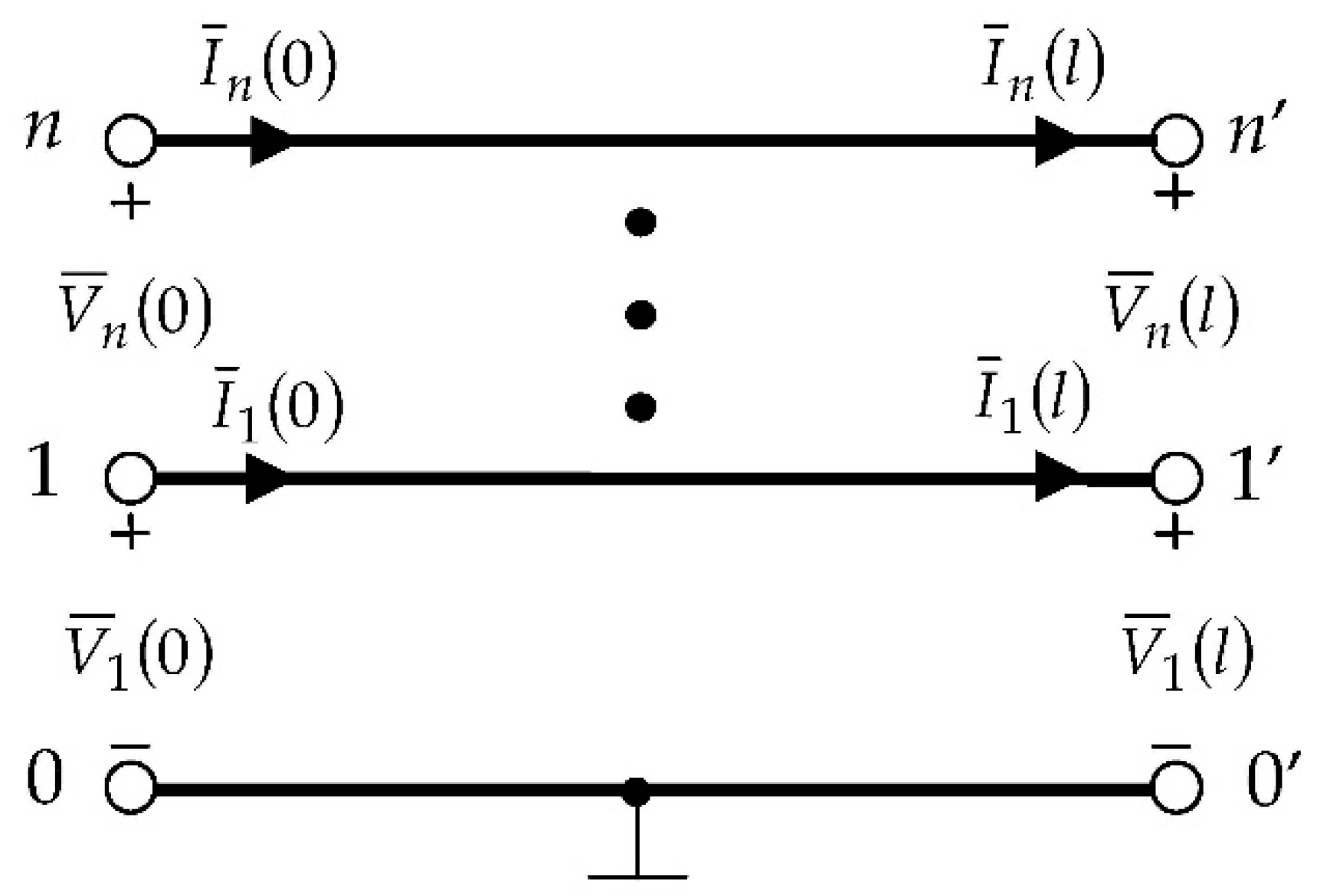
Let us consider a uniform $\left(n+1\right)$-conductor transmission line with distribution parameters immersed in a homogenous medium in an AC state at the angular frequency $\omega$. The line, having the length l, is shown in Figure 1, where ${\overline{V}}_1\left(0\right)$,…, ${\overline{V}}_n\left(0\right)$, ${\overline{I}}_1\left(0\right)$,…, ${\overline{I}}_n\left(0\right)$ are the phasors of the voltages and currents at the beginning of the line, whereas ${\overline{V}}_1\left(l\right)$,…, ${\overline{V}}_n\left(l\right)$, ${\overline{I}}_1\left(l\right)$,…, ${\overline{I}}_n\left(l\right)$ are the phasors of the voltages and currents at the end of the line. The line is specified by its per–unit–length (p–u–l) parameters $r_{\mathrm{o}},r_1,\dots ,r_n,l_{ij},g_{ij},c_{ij}$, $i,j=1,\dots ,n$ where $l_{ij}=l_{ji}$, $g_{ij}=g_{ji}$, $c_{ij}=c_{ji}$. They appear in the resistance, inductance, conductance, and capacitance $n\times n$ matrices R, L, G, and C. These matrices are components of the impedance and admittance $n\times n$ matrices $\overline{Z}=R+\mathrm{j}\omega L$, $\overline{Y}=G+\mathrm{j}\omega C$.

The line can be described by chain equations [28]:

$$\overline{V}\left(l\right)=\left({\overline{Z}}_C{\overline{T}}_I\left(\cos \mathrm{h}\overline{\gamma }l\right){\overline{T}}_I^{-1}{\overline{Z}}_C^{-1}\right)\overline{V}\left(0\right)-\left({\overline{Z}}_C{\overline{T}}_I\left(\sin \mathrm{h}\overline{\gamma }l\right){\overline{T}}_I^{-1}\right)\overline{I}\left(0\right)$$

(1)

$$\overline{I}\left(l\right)=-\left({\overline{T}}_I\left(\sin \mathrm{h}\overline{\gamma }l\right){\overline{T}}_I^{-1}{\overline{Z}}_C^{-1}\right)\overline{V}\left(0\right)+\left({\overline{T}}_I\left(\cos \mathrm{h}\overline{\gamma }l\right){\overline{T}}_I^{-1}\right)\overline{I}\left(0\right)$$

(2)

where

$$\overline{V}\left(0\right)=\left[\begin{array}{c}{\overline{V}}_1\left(0\right)\\ ⋮\\ {\overline{V}}_n\left(0\right)\end{array}\right],\overline{I}\left(0\right)=\left[\begin{array}{c}{\overline{I}}_1\left(0\right)\\ ⋮\\ {\overline{I}}_n\left(0\right)\end{array}\right],\overline{V}\left(l\right)=\left[\begin{array}{c}{\overline{V}}_1\left(l\right)\\ ⋮\\ {\overline{V}}_n\left(l\right)\end{array}\right],\overline{I}\left(l\right)=\left[\begin{array}{c}{\overline{I}}_1\left(l\right)\\ ⋮\\ {\overline{I}}_n\left(l\right)\end{array}\right].$$

${\overline{T}}_I$ is an $n\times n$ complex modal matrix, $\overline{\gamma }$ is an $n\times n$ diagonal matrix having complex diagonal elements ${\overline{\gamma }}_1,\dots ,{\overline{\gamma }}_n$, $\cos \mathrm{h}\overline{\gamma }l=\mathrm{diag}\left(\cos \mathrm{h}{\overline{\gamma }}_{1}l,\dots ,\cos \mathrm{h}{\overline{\gamma }}_{n}l\right)$, $\sin \mathrm{h}\overline{\gamma }l=\mathrm{diag}\left(\sin \mathrm{h}{\overline{\gamma }}_{1}l,\dots ,\sin \mathrm{h}{\overline{\gamma }}_{n}l\right)$, and ${\overline{Z}}_C={\overline{Y}}^{-1}{\overline{T}}_I\overline{\gamma }{\overline{T}}_I^{-1}$ is an $n\times n$ characteristic impedance matrix [28]. All the matrices can be determined having p–u–l parameters, and they do not depend on the line length l. Equations (1) and (2) express the voltage and current phasors at the end of a line in terms of the voltage and current phasors at the beginning of the line. The derivation of these equations is presented in detail in reference [28]. Similarly, we write the equations expressing the voltage and current phasors at the beginning of the line in terms of the voltage and current phasors at the end of the line, as follows,

$$\overline{V}\left(0\right)=\left({\overline{Z}}_C{\overline{T}}_I\left(\cos \mathrm{h}\overline{\gamma }l\right){\overline{T}}_I^{-1}{\overline{Z}}_C^{-1}\right)\overline{V}\left(l\right)+\left({\overline{Z}}_C{\overline{T}}_I\left(\sin \mathrm{h}\overline{\gamma }l\right){\overline{T}}_I^{-1}\right)\overline{I}\left(l\right)$$

(3)

$$\overline{I}\left(0\right)=\left({\overline{T}}_I\left(\sin \mathrm{h}\overline{\gamma }l\right){\overline{T}}_I^{-1}{\overline{Z}}_C^{-1}\right)\overline{V}\left(l\right)+\left({\overline{T}}_I\left(\cos \mathrm{h}\overline{\gamma }l\right){\overline{T}}_I^{-1}\right)\overline{I}\left(l\right).$$

(4)

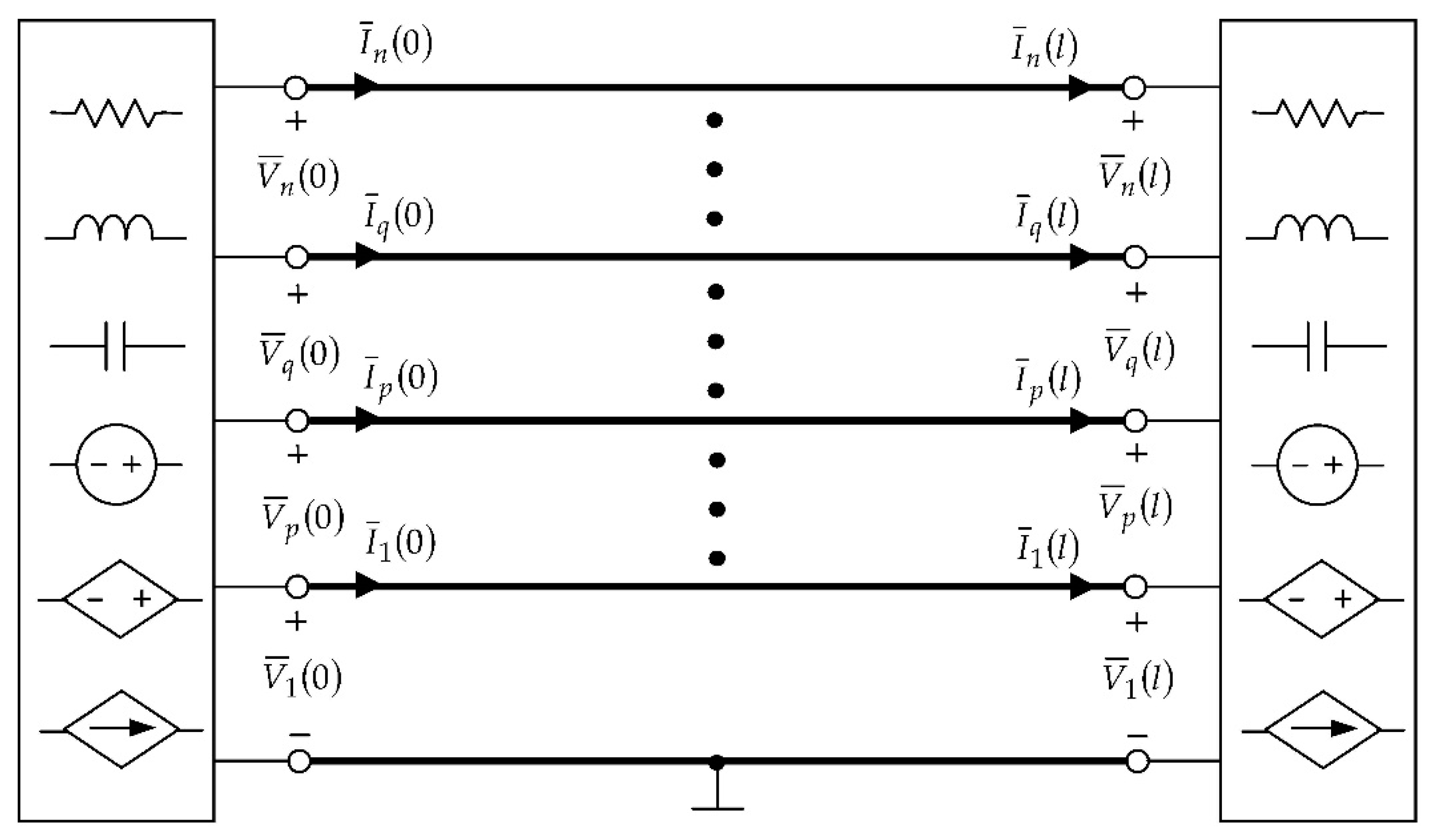
We wish to diagnose a fault in the given distributed parameter $\left(n+1\right)$-conductor transmission line terminated at the left and right ends by the lumped circuits, as shown in Figure 2. The p–u–l parameters and the length l of the line are known. The soft short can occur between any pair of the $\left(n+1\right)$ conductors $0,1,\dots ,n$. It is simulated by a low resistor $R_S\in \left[R_S^{-},R_S^{+}\right]$, where $R_S^{-}=1\mathsf{\Omega }$, $R_S^{+}=1000\mathsf{\Omega }$. The soft open fault can occur along any of the conductors $1,\dots ,n$ and is simulated by a high resistor $R_{\mathrm{o}}\in \left[R_{\mathrm{o}}^{-},R_{\mathrm{o}}^{+}\right]$ where $R_{\mathrm{o}}^{-}=100\mathrm{k}\mathsf{\Omega }$, $R_{\mathrm{o}}^{+}=10\mathrm{M}\mathsf{\Omega }$. The open fault is represented by resistor $R_{\mathrm{o}}$ whose resistance tends to infinity.

3. Soft Short Fault Diagnosis

The single soft short diagnosis encompasses the location of the fault by determining the pair of bridged conductors and the distance $\widehat{l}$ from the beginning of the line to the point where it takes place and estimating the resistance $R_S$.

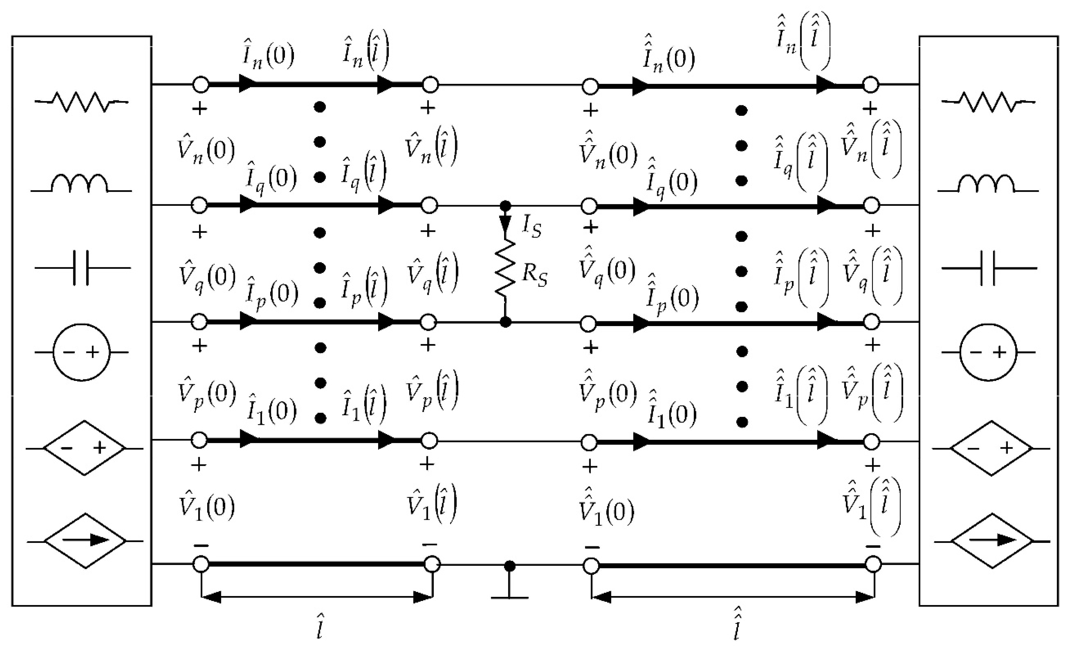
Assume that the soft short occurs between the conductors p and q $\left(p\ne 0,q\ne 0\right)$ at a distance $\widehat{l}$ from the beginning of the line, where $0<\widehat{l}<l$. To diagnose this fault, we consider the line as a cascade-connection of two lines having the lengths $\widehat{l}$ and $\widehat{\widehat{l}}$, where $\widehat{l}+\widehat{\widehat{l}}=l$, as demonstrated in Figure 3. In this figure, the voltage and current phasors relating to the left line are labeled using the hat symbol, while the ones relating to the right line are labeled using the double hat symbol.

The diagnostic method proposed in this paper is based on a measurement test performed in the AC state at the angular frequency $\omega$. In the course of this test, the voltage phasors at both ends of the line ${\widehat{V}}_1\left(0\right)$,…, ${\widehat{V}}_n\left(0\right)$, ${\widehat{\widehat{V}}}_1\left(\widehat{\widehat{l}}\right)$,…, ${\widehat{\widehat{V}}}_n\left(\widehat{\widehat{l}}\right)$ are measured and recorded. These voltages are used to calculate the current phasors ${\widehat{I}}_1\left(0\right)$,…, ${\widehat{I}}_n\left(0\right)$, ${\widehat{\widehat{I}}}_1\left(\widehat{\widehat{l}}\right)$,..., ${\widehat{\widehat{I}}}_n\left(\widehat{\widehat{l}}\right)$ by the analyses of the lumped circuits terminating the line.

We adapt Equations (1) and (2) to the left line in Figure 3

$$\widehat{V}\left(\widehat{l}\right)=\left[\begin{array}{c}{\widehat{V}}_1\left(\widehat{l}\right)\\ ⋮\\ {\widehat{V}}_n\left(\widehat{l}\right)\end{array}\right]=\left({\overline{Z}}_C{\overline{T}}_I\left(\cos \mathrm{h}\overline{\gamma }\widehat{l}\right){\overline{T}}_I^{-1}{\overline{Z}}_C^{-1}\right)\widehat{V}\left(0\right)-\left({\overline{Z}}_C{\overline{T}}_I\left(\sin \mathrm{h}\overline{\gamma }\widehat{l}\right){\overline{T}}_I^{-1}\right)\widehat{I}\left(0\right)=\left[\begin{array}{c}{\widehat{f}}_v^{\left(1\right)}\left(\widehat{l}\right)\\ ⋮\\ {\widehat{f}}_v^{\left(n\right)}\left(\widehat{l}\right)\end{array}\right]$$

(5)

$$\widehat{I}\left(\widehat{l}\right)=\left[\begin{array}{c}{\widehat{I}}_1\left(\widehat{l}\right)\\ ⋮\\ {\widehat{I}}_n\left(\widehat{l}\right)\end{array}\right]=-\left({\overline{T}}_I\left(\sin \mathrm{h}\overline{\gamma }\widehat{l}\right){\overline{T}}_I^{-1}{\overline{Z}}_C^{-1}\right)\widehat{V}\left(0\right)+\left({\overline{T}}_I\left(\cos \mathrm{h}\overline{\gamma }\widehat{l}\right){\overline{T}}_I^{-1}\right)\widehat{I}\left(0\right)=\left[\begin{array}{c}{\widehat{f}}_i^{\left(1\right)}\left(\widehat{l}\right)\\ ⋮\\ {\widehat{f}}_i^{\left(n\right)}\left(\widehat{l}\right)\end{array}\right]$$

(6)

where

$$\widehat{V}\left(0\right)=\left[\begin{array}{c}{\widehat{V}}_1\left(0\right)\\ ⋮\\ {\widehat{V}}_n\left(0\right)\end{array}\right]\mathrm{and}\widehat{I}\left(0\right)=\left[\begin{array}{c}{\widehat{I}}_1\left(0\right)\\ ⋮\\ {\widehat{I}}_n\left(0\right)\end{array}\right]$$

are given. Since the p–u–l parameters of the line are known, the matrices ${\overline{Z}}_C$, ${\overline{T}}_I$, and $\overline{\gamma }$ can be determined, and the expressions describing the line are functions of $\widehat{l}$ only, which are denoted by ${\widehat{f}}_v^{\left(1\right)}\left(\widehat{l}\right),\dots ,{\widehat{f}}_v^{\left(n\right)}\left(\widehat{l}\right)$ and ${\widehat{f}}_i^{\left(1\right)}\left(\widehat{l}\right),\dots ,{\widehat{f}}_i^{\left(n\right)}\left(\widehat{l}\right)$.

Equations (3) and (4) adapted to the right line in Figure 3 are as follows

$$\widehat{\widehat{V}}\left(0\right)=\left[\begin{array}{c}{\widehat{\widehat{V}}}_1\left(0\right)\\ ⋮\\ {\widehat{\widehat{V}}}_n\left(0\right)\end{array}\right]=\left({\overline{Z}}_C{\overline{T}}_I\left(\cos \mathrm{h}\overline{\gamma }\widehat{\widehat{l}}\right){\overline{T}}_I^{-1}{\overline{Z}}_C^{-1}\right)\widehat{\widehat{V}}\left(\widehat{\widehat{l}}\right)+\left({\overline{Z}}_C{\overline{T}}_I\left(\sin \mathrm{h}\overline{\gamma }\widehat{\widehat{l}}\right){\overline{T}}_I^{-1}\right)\widehat{\widehat{I}}\left(\widehat{\widehat{l}}\right)=\left[\begin{array}{c}{\widehat{\widehat{f}}}_v^{\left(1\right)}\left(\widehat{\widehat{l}}\right)\\ ⋮\\ {\widehat{\widehat{f}}}_v^{\left(n\right)}\left(\widehat{\widehat{l}}\right)\end{array}\right]$$

(7)

$$\widehat{\widehat{I}}\left(0\right)=\left[\begin{array}{c}{\widehat{\widehat{I}}}_1\left(0\right)\\ ⋮\\ {\widehat{\widehat{I}}}_n\left(0\right)\end{array}\right]=\left({\overline{T}}_I\left(\sin \mathrm{h}\overline{\gamma }\widehat{\widehat{l}}\right){\overline{T}}_I^{-1}{\overline{Z}}_C^{-1}\right)\widehat{\widehat{V}}\left(\widehat{\widehat{l}}\right)+\left({\overline{T}}_I\left(\cos \mathrm{h}\overline{\gamma }\widehat{\widehat{l}}\right){\overline{T}}_I^{-1}\right)\widehat{\widehat{I}}\left(\widehat{\widehat{l}}\right)=\left[\begin{array}{c}{\widehat{\widehat{f}}}_i^{\left(1\right)}\left(\widehat{\widehat{l}}\right)\\ ⋮\\ {\widehat{\widehat{f}}}_i^{\left(n\right)}\left(\widehat{\widehat{l}}\right)\end{array}\right]$$

(8)

where

$$\widehat{\widehat{V}}\left(\widehat{\widehat{l}}\right)=\left[\begin{array}{c}{\widehat{\widehat{V}}}_1\left(\widehat{\widehat{l}}\right)\\ ⋮\\ {\widehat{\widehat{V}}}_n\left(\widehat{\widehat{l}}\right)\end{array}\right]\mathrm{and}\widehat{\widehat{I}}\left(\widehat{\widehat{l}}\right)=\left[\begin{array}{c}{\widehat{\widehat{I}}}_1\left(\widehat{\widehat{l}}\right)\\ ⋮\\ {\widehat{\widehat{I}}}_n\left(\widehat{\widehat{l}}\right)\end{array}\right]$$

are provided by the measurement test and the analysis of the right termination of the line. Likewise, as in the cases of Equations (5) and (6), the functions on the right sides depend on the length of the line $\widehat{\widehat{l}}$ only. Applying the basic circuit laws in the circuit of Figure 3, we arrive at the set of $2n$ equations

$${\widehat{V}}_m\left(\widehat{l}\right)={\widehat{\widehat{V}}}_m\left(0\right)\hspace{1em}\mathrm{for}\hspace{1em}m\in \left\{1,\dots ,n\right\},$$

(9)

$${\widehat{I}}_m\left(\widehat{l}\right)={\widehat{\widehat{I}}}_m\left(0\right)\hspace{1em}\mathrm{for}\hspace{1em}m\in \left\{1,\dots ,n\right\},m\ne p,m\ne q,$$

(10)

$${\widehat{I}}_p\left(\widehat{l}\right)={\widehat{\widehat{I}}}_p\left(0\right)-\frac{1}{R_S}\left({\widehat{V}}_q\left(\widehat{l}\right)-{\widehat{V}}_p\left(\widehat{l}\right)\right),$$

(11)

$${\widehat{I}}_q\left(\widehat{l}\right)={\widehat{\widehat{I}}}_q\left(0\right)+\frac{1}{R_S}\left({\widehat{V}}_q\left(\widehat{l}\right)-{\widehat{V}}_p\left(\widehat{l}\right)\right).$$

(12)

The voltages and currents that appear in Equations (9)–(12) will be replaced by the functions that are defined in Equations (5)–(8). In addition, the length $\widehat{\widehat{l}}$ will be expressed in terms of $\widehat{l}$, $\widehat{\widehat{l}}=l-\widehat{l}$. Then, the system of $2n$ diagnostic equations arises

$${\widehat{f}}_v^{\left(m\right)}\left(\widehat{l}\right)-{\widehat{\widehat{f}}}_v^{\left(m\right)}\left(l-\widehat{l}\right)=0\hspace{1em}\mathrm{for}\hspace{1em}m\in \left\{1,\dots ,n\right\},$$

(13)

$${\widehat{f}}_i^{\left(m\right)}\left(\widehat{l}\right)-{\widehat{\widehat{f}}}_i^{\left(m\right)}\left(l-\widehat{l}\right)=0\hspace{1em}\mathrm{for}\hspace{1em}m\in \left\{1,\dots ,n\right\},m\ne p,m\ne q,$$

(14)

$${\widehat{f}}_v^{\left(p\right)}\left(\widehat{l}\right)-{\widehat{f}}_v^{\left(q\right)}\left(\widehat{l}\right)-R_S\left({\widehat{f}}_i^{\left(p\right)}\left(\widehat{l}\right)-{\widehat{\widehat{f}}}_i^{\left(p\right)}\left(l-\widehat{l}\right)\right)=0,$$

(15)

$${\widehat{f}}_v^{\left(q\right)}\left(\widehat{l}\right)-{\widehat{f}}_v^{\left(p\right)}\left(\widehat{l}\right)-R_S\left({\widehat{f}}_i^{\left(q\right)}\left(\widehat{l}\right)-{\widehat{\widehat{f}}}_i^{\left(q\right)}\left(l-\widehat{l}\right)\right)=0.$$

(16)

To simplify notation, the system of Equations (13) and (14) will be presented as

$$\begin{array}{c}{\tilde{g}}_1\left(\widehat{l}\right)=0\\ ⋮\\ {\tilde{g}}_{2n-2}\left(\widehat{l}\right)=0\end{array},$$

(17)

and the system of Equations (15) and (16) will be presented as

$$\begin{array}{c}{\tilde{\tilde{g}}}_1\left(\widehat{l},R_S\right)=0\\ {\tilde{\tilde{g}}}_2\left(\widehat{l},R_S\right)=0.\end{array}$$

(18)

Functions ${\tilde{g}}_1,\cdots ,{\tilde{g}}_{2n-2},{\tilde{\tilde{g}}}_1,{\tilde{\tilde{g}}}_2$ are complex and strongly nonlinear. The solution of the set of Equations (17) and (18), $\widehat{l}$ and $R_S$, determines the location of the fault and its value.

Similarly, the soft short between an arbitrary conductor $q\in \left\{1,\dots ,n\right\}$ and the reference conductor 0 can be diagnosed.

4. Solving the Diagnostic Equations

The numerical method described in the sequel relates to the diagnostic equations corresponding to the soft short occurring between conductors p and q, where $p\ne 0$ and $q\ne 0$. The soft short between conductors q and $p=0$ requires obvious slight modification of the method.

4.1. Iterative Method for Solving Systems of Nonlinear Complex Equations

Let us consider the equation

$$g\left(x\right)=0$$

(19)

where $x={\left[x_1\cdots x_s\right]}^{\mathrm{T}}$ is a vector whose elements are real variables, T denotes transposition, $g\left(x\right)={\left[g_1\left(x\right)\cdots g_r\left(x\right)\right]}^{\mathrm{T}}$ is a function mapping $R^s$ into $C^r$, consisting of r nonlinear complex functions of x, where $2r>s$, and 0 is the zero vector of order $r\times 1$. To solve Equation (19) using an iterative method, $g\left(x\right)$ is linearized about $x^{\left(k\right)}$, where k is the indexof iteration, and the linear equation is solved with respect to $x^{\left(k+1\right)}$ at the $\left(k+1\right)$st iteration

$$g\left(x^{\left(k\right)}\right)+D\left(x^{\left(k\right)}\right)\left(x^{\left(k+1\right)}-x^{\left(k\right)}\right)=0$$

(20)

where $x^{\left(k\right)}={\left[x_1^{\left(k\right)}\cdots x_s^{\left(k\right)}\right]}^{\mathrm{T}}$, $x^{\left(k+1\right)}={\left[x_1^{\left(k+1\right)}\cdots x_s^{\left(k+1\right)}\right]}^{\mathrm{T}}$,

$$D\left(x^{\left(k\right)}\right)=\left[\begin{array}{c}{d}_1\left(x^{\left(k\right)}\right)\\ ⋮\\ d_r\left(x^{\left(k\right)}\right)\end{array}\right]$$

(21)

where $d_i\left(x^{\left(k\right)}\right)=\left[\frac{\partial g_i}{\partial x_1}\left(x^{\left(k\right)}\right)\cdots \frac{\partial g_i}{\partial x_s}\left(x^{\left(k\right)}\right)\right]$, $i=1,\dots ,r$. Thus, $D\left(x^{\left(k\right)}\right)$ for given $x^{\left(k\right)}$ is an $r\times s$ matrix whose elements are complex numbers. Let us present these numbers in rectangular form and rewrite $D\left(x^{\left(k\right)}\right)$ as

$$D\left(x^{\left(k\right)}\right)=\mathrm{Re}D\left(x^{\left(k\right)}\right)+\mathrm{jIm}D\left(x^{\left(k\right)}\right)$$

(22)

where j is the imaginary unit. Similarly, we write

$$g\left(x^{\left(k\right)}\right)=\mathrm{Re}g\left(x^{\left(k\right)}\right)+\mathrm{jIm}g\left(x^{\left(k\right)}\right).$$

(23)

Using (22) and (23), we rewrite (20) as

$$\begin{array}{l}\left[\mathrm{Re}D\left(x^{\left(k\right)}\right)\right]\left(x^{\left(k+1\right)}-x^{\left(k\right)}\right)+\mathrm{j}\left[\mathrm{Im}D\left(x^{\left(k\right)}\right)\right]\left(x^{\left(k+1\right)}-x^{\left(k\right)}\right)=-\mathrm{Re}g\left(x^{\left(k\right)}\right)-\mathrm{jIm}g\left(x^{\left(k\right)}\right)\end{array}$$

(24)

where $x^{\left(k\right)}$ and $x^{\left(k+1\right)}$ consists of real numbers. Equalizing the real and imaginary parts, we obtain

$$\begin{array}{l}\left[\mathrm{Re}D\left(x^{\left(k\right)}\right)\right]\left(x^{\left(k+1\right)}-x^{\left(k\right)}\right)=-\mathrm{Re}g\left(x^{\left(k\right)}\right)\\ \left[\mathrm{Im}D\left(x^{\left(k\right)}\right)\right]\left(x^{\left(k+1\right)}-x^{\left(k\right)}\right)=-\mathrm{Im}g\left(x^{\left(k\right)}\right)\end{array}$$

(25)

which can be presented in the form

$$\left[\begin{array}{c}\mathrm{Re}D\left(x^{\left(k\right)}\right)\\ \mathrm{Im}D\left(x^{\left(k\right)}\right)\end{array}\right]\left(x^{\left(k+1\right)}-x^{\left(k\right)}\right)=-\left[\begin{array}{c}\mathrm{Re}g\left(x^{\left(k\right)}\right)\\ \mathrm{Im}g\left(x^{\left(k\right)}\right)\end{array}\right],$$

(26)

where $\left[\begin{array}{c}\mathrm{Re}D\left(x^{\left(k\right)}\right)\\ \mathrm{Im}D\left(x^{\left(k\right)}\right)\end{array}\right]$ is a real $2r\times s$ matrix and $\left[\begin{array}{c}\mathrm{Re}g\left(x^{\left(k\right)}\right)\\ \mathrm{Im}g\left(x^{\left(k\right)}\right)\end{array}\right]$ is a real $2r\times 1$ vector. Thus, Equation (26) represents an overdetermined system of $2r$ real equations in $s<2r$ unknown real variables, which are elements of vector $x^{\left(k+1\right)}$. To solve this overdetermined system, the normal equation method will be used. For this purpose, both sides of Equation (26) are multiplied by the matrix $\left[\mathrm{Re}{D}^{\mathrm{T}}\left(x^{\left(k\right)}\right)\mathrm{Im}{D}^{\mathrm{T}}\left(x^{\left(k\right)}\right)\right]$, leading to the iteration equation

$$A\left(x^{\left(k\right)}\right)\left(x^{\left(k+1\right)}-x^{\left(k\right)}\right)=b\left(x^{\left(k\right)}\right),$$

(27)

where

$$A\left(x^{\left(k\right)}\right)=\left[\mathrm{Re}{D}^{\mathrm{T}}\left(x^{\left(k\right)}\right)\mathrm{Im}{D}^{\mathrm{T}}\left(x^{\left(k\right)}\right)\right]\left[\begin{array}{c}\mathrm{Re}D\left(x^{\left(k\right)}\right)\\ \mathrm{Im}D\left(x^{\left(k\right)}\right)\end{array}\right],$$

(28)

$$b\left(x^{\left(k\right)}\right)=-\left[\mathrm{Re}{D}^{\mathrm{T}}\left(x^{\left(k\right)}\right)\mathrm{Im}{D}^{\mathrm{T}}\left(x^{\left(k\right)}\right)\right]\left[\begin{array}{c}\mathrm{Re}g\left(x^{\left(k\right)}\right)\\ \mathrm{Im}g\left(x^{\left(k\right)}\right)\end{array}\right].$$

(29)

Since the order of $D\left(x^{\left(k\right)}\right)$ is $r\times s$, the order of the matrix $\mathrm{Re}{D}^{\mathrm{T}}\left(x^{\left(k\right)}\right)$ and the matrix $\mathrm{Im}{D}^{\mathrm{T}}\left(x^{\left(k\right)}\right)$ is $s\times r$. Their elements are real numbers. Thus, the right side of (28), as the product of two real matrices of orders $s\times 2r$ and $2r\times s$ is a real $s\times s$ matrix. Similarly, on the right side of (29), there is the product of the $s\times 2r$ matrix and $2r\times 1$ vector giving $s\times 1$ vector.

Thus, the iteration Equation (27) represents s individual real linear equations in s real unknown variables. If $\det A\left(x^{\left(k\right)}\right)\ne 0$, this equation can be uniquely solved finding $x^{\left(k+1\right)}$ at the $\left(k+1\right)$st iteration. The iteration process is running until $\Vert x^{\left(k+1\right)}-x^{\left(k\right)}\Vert <\tilde{\epsilon }$ and $\Vert g_{\mathrm{mag}}\left(x^{\left(k+1\right)}\right)\Vert <\tilde{\tilde{\epsilon }}$, where $\tilde{\epsilon }$ and $\tilde{\tilde{\epsilon }}$ are the convergence tolerances, $\Vert \cdot \Vert$ is the Euclidean norm, and $g_{\mathrm{mag}}\left(x^{\left(k+1\right)}\right)={\left[\left|g_1\left(x^{\left(k+1\right)}\right)\right|\cdots \left|g_r\left(x^{\left(k+1\right)}\right)\right|\right]}^{\mathrm{T}}$, i.e., $\Vert g_{\mathrm{mag}}\left(x^{\left(k+1\right)}\right)\Vert =\sqrt{{\left|g_1\left(x^{\left(k+1\right)}\right)\right|}^2\cdots {\left|g_r\left(x^{\left(k+1\right)}\right)\right|}^2}$.

4.1.1. First Particular Case

If $s=1$, vector x reduces to scalar x and $g\left(x\right)={\left[g_1\left(x\right)\dots g_r\left(x\right)\right]}^{\mathrm{T}}$. Thus, Equation (19) represents a system of r equations in one real variable x. In such case $D\left(x^{\left(k\right)}\right)={\left[\frac{\mathrm{d}{g}_1}{\mathrm{d}x}\left(x^{\left(k\right)}\right)\cdots \frac{\mathrm{d}{g}_r}{\mathrm{d}x}\left(x^{\left(k\right)}\right)\right]}^{\mathrm{T}}$ and matrix $A\left(x^{\left(k\right)}\right)$, according to Equation (28), reduces to the real number

$$A\left(x^{\left(k\right)}\right)=c\left(x^{\left(k\right)}\right)c^{\mathrm{T}}\left(x^{\left(k\right)}\right),$$

(30)

where

$$c\left(x^{\left(k\right)}\right)=\left[\mathrm{Re}\frac{\mathrm{d}{g}_1}{\mathrm{d}x}\left(x^{\left(k\right)}\right)\cdots \mathrm{Re}\frac{\mathrm{d}{g}_r}{\mathrm{d}x}\left(x^{\left(k\right)}\right)\mathrm{Im}\frac{\mathrm{d}{g}_1}{\mathrm{d}x}\left(x^{\left(k\right)}\right)\cdots \mathrm{Im}\frac{\mathrm{d}{g}_r}{\mathrm{d}x}\left(x^{\left(k\right)}\right)\right].$$

(31)

In addition, vector $b\left(x^{\left(k\right)}\right)$ defined by Equation (29) becomes the real number

$$b\left(x^{\left(k\right)}\right)=-c\left(x^{\left(k\right)}\right){\left[\mathrm{Re}{g}_1\left(x^{\left(k\right)}\right)\cdots \mathrm{Re}{g}_r\left(x^{\left(k\right)}\right)\mathrm{Im}{g}_1\left(x^{\left(k\right)}\right)\cdots \mathrm{Im}{g}_r\left(x^{\left(k\right)}\right)\right]}^{\mathrm{T}},$$

(32)

and the iteration Equation (27) reduces to the formula

$$x^{\left(k+1\right)}=x^{\left(k\right)}+\frac{b\left(x^{\left(k\right)}\right)}{c\left(x^{\left(k\right)}\right)c^{\mathrm{T}}\left(x^{\left(k\right)}\right)}{.}^{}$$

(33)

4.1.2. Second Particular Case

If $r=2$ and $s=2$ then $x={\left[x_1{x}_2\right]}^{\mathrm{T}}$ and

$$D\left(x^{\left(k\right)}\right)=\left[\begin{array}{cc}\frac{\partial g_1}{\partial x_1}\left(x^{\left(k\right)}\right)& \frac{\partial g_1}{\partial x_2}\left(x^{\left(k\right)}\right)\\ \frac{\partial g_2}{\partial x_1}\left(x^{\left(k\right)}\right)& \frac{\partial g_2}{\partial x_2}\left(x^{\left(k\right)}\right)\end{array}\right],$$

(34)

according to Equation (28), $A\left(x^{\left(k\right)}\right)$ is a $2\times 2$ real matrix

$$A\left(x^{\left(k\right)}\right)=H^{\mathrm{T}}\left(x^{\left(k\right)}\right)H\left(x^{\left(k\right)}\right),$$

(35)

where

$$H\left(x^{\left(k\right)}\right)=\left[\begin{array}{cc}\mathrm{Re}\frac{\partial g_1}{\partial x_1}\left(x^{\left(k\right)}\right)& \mathrm{Re}\frac{\partial g_1}{\partial x_2}\left(x^{\left(k\right)}\right)\\ \mathrm{Re}\frac{\partial g_2}{\partial x_1}\left(x^{\left(k\right)}\right)& \mathrm{Re}\frac{\partial g_2}{\partial x_2}\left(x^{\left(k\right)}\right)\\ \mathrm{Im}\frac{\partial g_1}{\partial x_1}\left(x^{\left(k\right)}\right)& \mathrm{Im}\frac{\partial g_1}{\partial x_2}\left(x^{\left(k\right)}\right)\\ \mathrm{Im}\frac{\partial g_2}{\partial x_1}\left(x^{\left(k\right)}\right)& \mathrm{Im}\frac{\partial g_2}{\partial x_2}\left(x^{\left(k\right)}\right)\end{array}\right]$$

(36)

and $b\left(x^{\left(k\right)}\right)$, according to Equation (29), is a $2\times 1$ real vector

$$b\left(x^{\left(k\right)}\right)=-H^{\mathrm{T}}{\left[\mathrm{Re}{g}_1\left(x^{\left(k\right)}\right)\mathrm{Re}{g}_2\left(x^{\left(k\right)}\right)\mathrm{Im}{g}_1\left(x^{\left(k\right)}\right)\mathrm{Im}{g}_2\left(x^{\left(k\right)}\right)\right]}^{\mathrm{T}}.$$

(37)

Thus, in this case, the iteration Equation (27) represents a system of two real linear equations in two real unknown variables $x_1^{\left(k+1\right)}$ and $x_2^{\left(k+1\right)}$.

4.2. Algorithm for Solving the Diagnostic Equations

To solve the system of diagnostic equations consisting of Equations (17) and (18), we consider first the system (17) of $2n-2$ equations with one variable $\widehat{l}$ and apply the iterative method described in Section 4.1.1. The iteration formula (33) adapted to Equation (17) has the form

$${\widehat{l}}^{\left(k+1\right)}={\widehat{l}}^{\left(k\right)}-\frac{{\displaystyle \sum _{i=1}^{2n-2}\left[\left(\mathrm{Re}\frac{\partial {\tilde{g}}_i}{\partial \widehat{l}}\left({\widehat{l}}^{\left(k\right)}\right)\right)\left(\mathrm{Re}{\tilde{g}}_i\left({\widehat{l}}^{\left(k\right)}\right)\right)+\left(\mathrm{Im}\frac{\partial {\tilde{g}}_i}{\partial \widehat{l}}\left({\widehat{l}}^{\left(k\right)}\right)\right)\left(\mathrm{Im}{\tilde{g}}_i\left({\widehat{l}}^{\left(k\right)}\right)\right)\right]}}{{\displaystyle \sum _{i=1}^{2n-2}\left[{\left(\mathrm{Re}\frac{\partial {\tilde{g}}_i}{\partial \widehat{l}}\left({\widehat{l}}^{\left(k\right)}\right)\right)}^2+{\left(\mathrm{Im}\frac{\partial {\tilde{g}}_i}{\partial \widehat{l}}\left({\widehat{l}}^{\left(k\right)}\right)\right)}^2\right]}}.$$

(38)

We choose ${\widehat{l}}^{\left(0\right)}=\frac{1}{2}l$ as the initial guess. The iteration ${\widehat{l}}^{\left(k+1\right)}$ that meets the convergence tolerances $\left|{\widehat{l}}^{\left(k+1\right)}-{\widehat{l}}^{\left(k\right)}\right|<\tilde{\epsilon }$ and $\Vert {\tilde{g}}_{\mathrm{mag}}\left({\widehat{l}}^{\left(k+1\right)}\right)\Vert <{\tilde{\tilde{\epsilon }}}_1$ is denoted by ${\widehat{l}}_1$.

Next, Equation (18) is solved, as described in Section 4.1.2 by substituting $x_1=\widehat{l}$ and $x_2=R_S$ starting with ${\widehat{l}}^{\left(0\right)}={\widehat{l}}_1$, $R_S^{\left(0\right)}=\frac{1}{2}\left(R_S^{-}+R_S^{+}\right)$. The iteration equation has the form

$$A\left({\widehat{l}}^{\left(k\right)},R_S^{\left(k\right)}\right)\left[\begin{array}{c}{\widehat{l}}^{\left(k+1\right)}-{\widehat{l}}^{\left(k\right)}\\ R_S^{\left(k+1\right)}-R_S^{\left(k\right)}\end{array}\right]=b\left({\widehat{l}}^{\left(k\right)},R_S^{\left(k\right)}\right),$$

(39)

where $A\left({\widehat{l}}^{\left(k\right)},R_S^{\left(k\right)}\right)$ is a $2\times 2$ real matrix (see Equation (35)) and $b\left({\widehat{l}}^{\left(k\right)},R_S^{\left(k\right)}\right)$ is a real $2\times 1$ vector (see Equation (37)). If the convergence tolerances are satisfied at $\left(k+1\right)$st iteration $\Vert {\left[{\widehat{l}}^{\left(k+1\right)}-{\widehat{l}}^{\left(k\right)}{R}_S^{\left(k+1\right)}-R_S^{\left(k\right)}\right]}^{\mathrm{T}}\Vert <\tilde{\epsilon }$ and $\Vert {\left[\left|{\tilde{\tilde{g}}}_1\left({\widehat{l}}^{\left(k+1\right)},R_S^{\left(k+1\right)}\right)\right|\left|{\tilde{\tilde{g}}}_2\left({\widehat{l}}^{\left(k+1\right)},R_S^{\left(k+1\right)}\right)\right|\right]}^{\mathrm{T}}\Vert <{\tilde{\tilde{\epsilon }}}_1$, then they constitute the solution of Equation (18) denoted by ${\widehat{l}}^{\ast }$, $R_S^{\ast }$. Furthermore, if $\Vert {\left[\left|{\tilde{g}}_1\left({\widehat{l}}^{\ast }\right)\right|\cdots \left|{\tilde{g}}_{2\mathrm{n}-2}\left({\widehat{l}}^{\ast }\right)\right|\left|{\tilde{\tilde{g}}}_1\left({\widehat{l}}^{\ast },R_S^{\ast }\right)\right|\left|{\tilde{\tilde{g}}}_2\left({\widehat{l}}^{\ast },R_S^{\ast }\right)\right|\right]}^{\mathrm{T}}\Vert <\tilde{\tilde{\epsilon }}$, then they form the solution of the diagnostic Equations (17) and (18).

If the iterative method does not meet the convergence tolerances in a preset maximum number of iterations $M_{\mathrm{it}}$, the method fails.

5. Some Remarks

Below, we explain how the diagnosis of the $\left(n+1\right)$-conductor transmission line is drawn from the proposed method.

5.1. Sketch of the Soft Short Diagnostic Procedure

• Perform the diagnostic test and record the measurement data.
• Have the p–u–l parameters of the given line determine the matrices $\overline{Z}$, $\overline{Y}$, ${\overline{T}}_I$, ${\overline{Z}}_C$, and $\overline{\gamma }$.
• Determine the currents entering and leaving the line by the analysis of the lumped terminations driven by the voltages measured in the course of the diagnostic test.
• Identify all pairs of the conductors where the soft shorts can occur. In the $\left(n+1\right)$-conductor line, the number of them is $N=\frac{\left(n+1\right)!}{\left(n-1\right)!2!}$.
• For each of the possible soft shorts, build the model of the faulty circuit as in Figure 3 and write the set of the diagnostic equations, similarly as Equations (13)–(16), and every time apply the numerical method described in Section 4. As a rule, the method finds the solution corresponding to the actual fault only and fails in the cases of the other $N-1$ virtual faults. Occasionally, the method gives also the solutions relating to certain virtual soft shorts that satisfy the diagnostic test. In such case, the diagnostic procedure provides the actual fault and one or more virtual faults. If the method finds a nonrealistic solution, it is discarded. If $R_S$ does not belong to the range $\left[R_S^{-},R_S^{+}\right]$, it is not classified as a soft short.

5.2. Open Fault Diagnosis

The method dedicated to soft shorts can be directly adapted to the diagnosis of soft open faults, which may occur along any of the conductors $1,\dots ,n$ and is simulated by a high resistor $R_{\mathrm{o}}$. Numerical experiments carried out in the circuits of Figure 4, Figure 5 and Figure 6, considering different values of $R_{\mathrm{o}}$ from the range $\left[100\mathrm{k}\mathsf{\Omega }–10\mathrm{M}\mathsf{\Omega }\right]$, reveal that the method correctly identifies the defected conductor and locates the point where the fault occurs (the distance $\widehat{l}$). Unfortunately, as a rule, it gives a wrong value of $R_{\mathrm{o}}$. The method is also able to find the correct value of $R_{\mathrm{o}}$ if the measurement accuracy while running the diagnostic test is very high. Unfortunately, assurance of such accuracy is impossible in real conditions. Therefore, the method is offered to the diagnosis of open faults rather than soft open faults and is limited to fault detection and location only. In such a case, it is very efficient as illustrated in Section 6, Example 4.

6. Examples

The method proposed in Section 3, Section 4 and Section 5 was implemented in the MATLAB environment, and the calculations were performed on PC with an Intel Core i7-6700 processor. To show the efficiency of the method, three numerical examples are presented.

6.1. Example 1

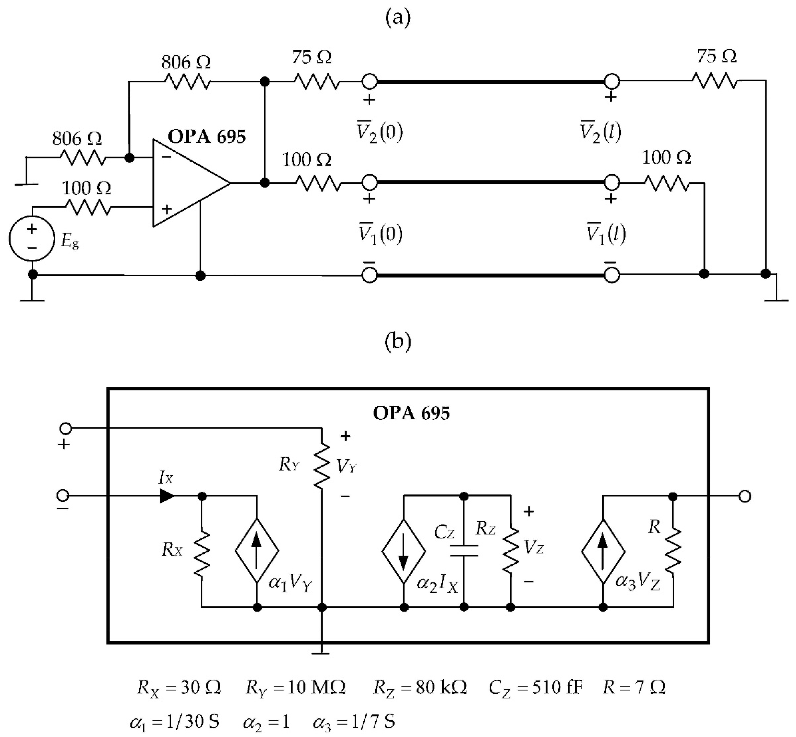
Let us consider the high-performance line driver with distribution amplifier features shown in Figure 4, including a current feedback operational amplifier, lumped elements, and DPMTL consisting of three conductors. The values of the lumped elements existing in the circuit and the current feedback operational amplifier model are indicated in the figure, whereas the p-u-l parameters of the DPMTL are as follows: $r_1=0.1437\mathsf{\Omega }/\mathrm{m}$, $r_2=0.1437\mathsf{\Omega }/\mathrm{m}$, $r_0=0$, $l_{11}=4.1185\cdot {10}^{-7}\mathrm{H}/\mathrm{m}$, $l_{22}=4.1185\cdot {10}^{-7}\mathrm{H}/\mathrm{m}$, $l_{12}=6.7294\cdot {10}^{-8}\mathrm{H}/\mathrm{m}$, $c_{11}=5.2176\cdot {10}^{-11}\mathrm{F}/\mathrm{m}$, $c_{22}=5.2176\cdot {10}^{-11}\mathrm{F}/\mathrm{m}$, $c_{12}=1.0190\cdot {10}^{-11}\mathrm{F}/\mathrm{m}$, $g_{11}=0.1049\mathrm{S}/\mathrm{m}$, $g_{22}=0.1049\mathrm{S}/\mathrm{m}$, and $g_{12}=0.0204\mathrm{S}/\mathrm{m}$. The length of the line is 0.4 m, the amplitude of the power supply voltage source $E_g$ is 2 V, the phase is $0^{\mathrm{o}}$, $f$ = 100 MHz. The accuracy of measurement of the voltage amplitudes is 0.1 mV and of the phases is ${0.01}^{\mathrm{o}}$. The end values of $R_S$ are equal to $R_S^{-}=1\mathsf{\Omega }$, $R_S^{+}=1000\mathsf{\Omega }$, the convergence tolerances are $\tilde{\epsilon }=0.001$, ${\tilde{\tilde{\epsilon }}}_1=0.01$, $\tilde{\tilde{\epsilon }}=0.02$, and the maximum number of iterations $M_{\mathrm{it}}=30$.

To illustrate the proposed method, 24 soft short faults occurring in DPMTL at $\widehat{l}=0.12\mathrm{m}$ and $\widehat{l}=0.30\mathrm{m}$ between different pairs of the conductors, for $R_s\in \left[1\mathsf{\Omega },1000\mathsf{\Omega }\right]$, were diagnosed. Statistical results are as follows. In 95.8%, the method correctly locates the fault and estimates its value, in 4.2%, the method finds the correct fault and a virtual fault. Outcomes of the diagnoses of 12 soft short faults are summarized in

Table 1. Outcomes of the soft shorts diagnoses in the circuit of Figure 4.

Number of the Fault	The Pair of Conductors Where the Actual Fault Occurs	Actual Value of ${\mathit{R}}_{\mathit{S}}$ (Ω)	Actual Value of $\widehat{\mathit{l}}$ (m)	Value of ${\mathit{R}}_{\mathit{S}}$ Given by the Method (Ω)	Value of $\widehat{\mathit{l}}$ Given by the Method (m)	Existence of Virtual Faults
1	0–1	20	0.12	20.00	0.1200	no
2	0–1	100	0.30	100.01	0.3001	no
3	0–1	850	0.12	852.53	0.1197	no
4	0–2	2	0.30	2.00	0.3000	no
5	0–2	50	0.12	49.99	0.1200	no
6	0–2	200	0.30	199.85	0.2998	no
7	0–2	600	0.12	600.90	0.1200	no
8	0–2	920	0.30	917.21	0.3009	no
9	1–2	2	0.12	2.02	0.1200	no
10	1–2	20	0.30	20.17	0.2998	yes
11	1–2	300	0.12	299.15	0.1207	no
12	1–2	750	0.30	757.90	0.2973	no

.

For each of the faults 1–9 and 11–12 presented in Table 1, the diagnostic method finds only the actual fault. The iterative method applied to all other possible faults is not convergent. For fault 10, the method finds the actual fault placed in Table 1 and the virtual fault occurring between the conductors 0 and 2: $R_S=510.60\mathsf{\Omega }$, $\widehat{l}=0.3358\mathrm{m}$.

The CPU time of each diagnosis, including the application of the numerical method described in Section 4 to all possible faults occurring between each pair of the conductors, does not exceed 0.40 s. For example, the CPU time of the diagnosis of fault 1 in Table 1 is equal to 0.23 s and that of fault 3 is equal to 0.30 s.

6.2. Example 2

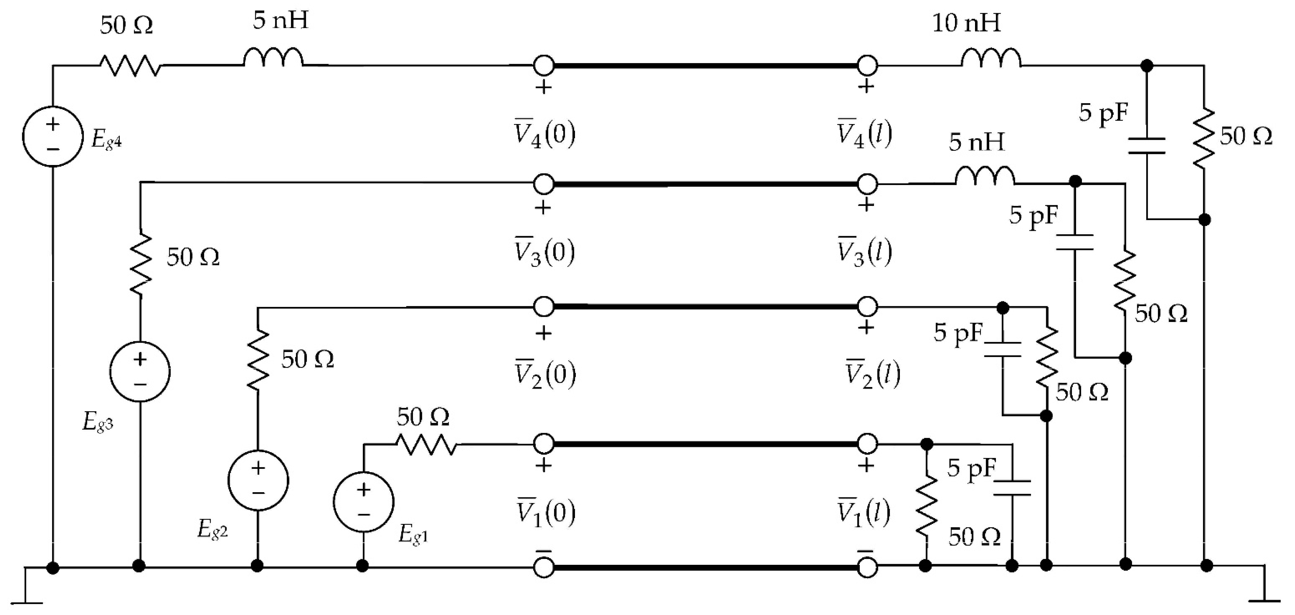
Let us consider the circuit of very high frequency shown in Figure 5, including a five-conductor transmission line with distribution parameters and lumped elements. The values of the lumped elements are indicated in the figure.

The DPMTL is specified by p-u-l parameters as follows: $r_1=r_2=r_3=r_4=0.7492\mathsf{\Omega }/\mathrm{m}$, $r_0=0$, $l_{11}=1.1983\cdot {10}^{-6}\mathrm{H}/\mathrm{m}$, $l_{22}=1.0832\cdot {10}^{-6}\mathrm{H}/\mathrm{m}$, $l_{33}=9.2104\cdot {10}^{-7}\mathrm{H}/\mathrm{m}$, $l_{44}=6.4377\cdot {10}^{-7}\mathrm{H}/\mathrm{m}$, $l_{12}=8.1887\cdot {10}^{-7}\mathrm{H}/\mathrm{m}$, $l_{13}=5.9915\cdot {10}^{-7}\mathrm{H}/\mathrm{m}$, $l_{14}=3.7942\cdot {10}^{-7}\mathrm{H}/\mathrm{m}$, $l_{23}=6.8024\cdot {10}^{-7}\mathrm{H}/\mathrm{m}$, $l_{24}=4.0298\cdot {10}^{-7}\mathrm{H}/\mathrm{m}$, $l_{34}=4.6052\cdot {10}^{-7}\mathrm{H}/\mathrm{m}$, $c_{11}=6.4044\cdot {10}^{-12}\mathrm{F}/\mathrm{m}$, $c_{22}=4.5726\cdot {10}^{-12}\mathrm{F}/\mathrm{m}$, $c_{33}=6.2537\cdot {10}^{-12}\mathrm{F}/\mathrm{m}$, $c_{44}=3.0312\cdot {10}^{-11}\mathrm{F}/\mathrm{m}$, $c_{12}=3.0312\cdot {10}^{-11}\mathrm{F}/\mathrm{m}$, $c_{13}=6.2537\cdot {10}^{-12}\mathrm{F}/\mathrm{m}$, $c_{14}=4.5727\cdot {10}^{-12}\mathrm{F}/\mathrm{m}$, $c_{23}=2.6941\cdot {10}^{-11}\mathrm{F}/\mathrm{m}$, $c_{24}=4.1807\cdot {10}^{-12}\mathrm{F}/\mathrm{m}$, $c_{34}=2.6941\cdot {10}^{-11}\mathrm{F}/\mathrm{m}$, $g_{11}=0.0091\mathrm{S}/\mathrm{m}$, $g_{22}=0.0065\mathrm{S}/\mathrm{m}$, $g_{33}=0.0088\mathrm{S}/\mathrm{m}$, $g_{44}=0.0428\mathrm{S}/\mathrm{m}$, $g_{12}=0.0428\mathrm{S}/\mathrm{m}$, $g_{13}=0.0088\mathrm{S}/\mathrm{m}$, $g_{14}=0.0065\mathrm{S}/\mathrm{m}$, $g_{23}=0.0381\mathrm{S}/\mathrm{m}$, $g_{24}=0.0059\mathrm{S}/\mathrm{m}$, and $g_{34}=0.0381\mathrm{S}/\mathrm{m}$. The length of the line is 0.5 m, the amplitudes of the power supply voltage sources are 5 V, the phases are $0^{\mathrm{o}}$, and $f$ = 100 MHz. The accuracy of measurement of the voltage amplitudes is 0.1 mV and of the phases is ${0.01}^{\mathrm{o}}$. The end values of $R_S$ are equal to $R_S^{-}=1\mathsf{\Omega }$, $R_S^{+}=1000\mathsf{\Omega }$, the convergence tolerances are $\tilde{\epsilon }=0.001$, ${\tilde{\tilde{\epsilon }}}_1=0.01$, and $\tilde{\tilde{\epsilon }}=0.02$, and the maximum number of iterations $M_{\mathrm{it}}=30$.

To illustrate the method, 20 soft short faults occurring in the DPMTL at $\widehat{l}=0.15\mathrm{m}$ and $\widehat{l}=0.40\mathrm{m}$ between different pairs of the conductors for $R_S\in \left[1\mathsf{\Omega },1000\mathsf{\Omega }\right]$ were diagnosed. In 15 cases (75%), the method correctly locates the fault and estimates its value; in one case (5%), the method correctly locates the actual fault and estimates its value but finds also a virtual fault; in two cases (10%), the method correctly locates the fault but gives its value inaccurately; in two cases (10%), the method fails. The results of the diagnoses of 10 soft short faults are presented in

Table 2. Results of soft short diagnoses in the circuit of Figure 5.

Number of the Fault	The Pair of Conductors Where the Actual Fault Occurs	Actual Value of ${\mathit{R}}_{\mathit{S}}$ (Ω)	Actual Value of $\widehat{\mathit{l}}$ (m)	Value of ${\mathit{R}}_{\mathit{S}}$ Given by the Method (Ω)	Value of $\widehat{\mathit{l}}$ Given by the Method (m)	Existence of Virtual Faults
1	0–1	2	0.40	1.86	0.4001	no
2	0–2	670	0.40	672.18	0.3991	no
3	0–3	470	0.15	469.44	0.1500	no
4	0–4	980	0.15	974.59	0.1504	no
5	1–2	150	0.15	159.57	0.1447	no
6	1–3	500	0.40	410.35	0.4021	no
7	1–4	15	0.40	15.17	0.3999	no
8	2–3	650	0.40	no solution
9	2–4	400	0.15	401.75	0.1492	no
10	3–4	50	0.40	49.89	0.4000	yes

. For faults 1–5, 7, and 9 presented in Table 2, the method finds only the actual fault and correctly estimates its location and value. For fault 6, the method finds the actual fault, but the estimated value of $R_S$ differs significantly from the actual one. For fault 8, the method fails. For fault 10, the method finds the actual fault placed in Table 2 and the virtual fault occurring between the conductors 1 and 2: $R_S=124.72\mathsf{\Omega }$, $\widehat{l}=0.3966\mathrm{m}.$ The CPU time of each diagnosis does not exceed 1.00 s. For example, the CPU time of the diagnosis of fault 1 in Table 2 is equal to 0.94 s and that of fault 3 is equal to 0.84 s.

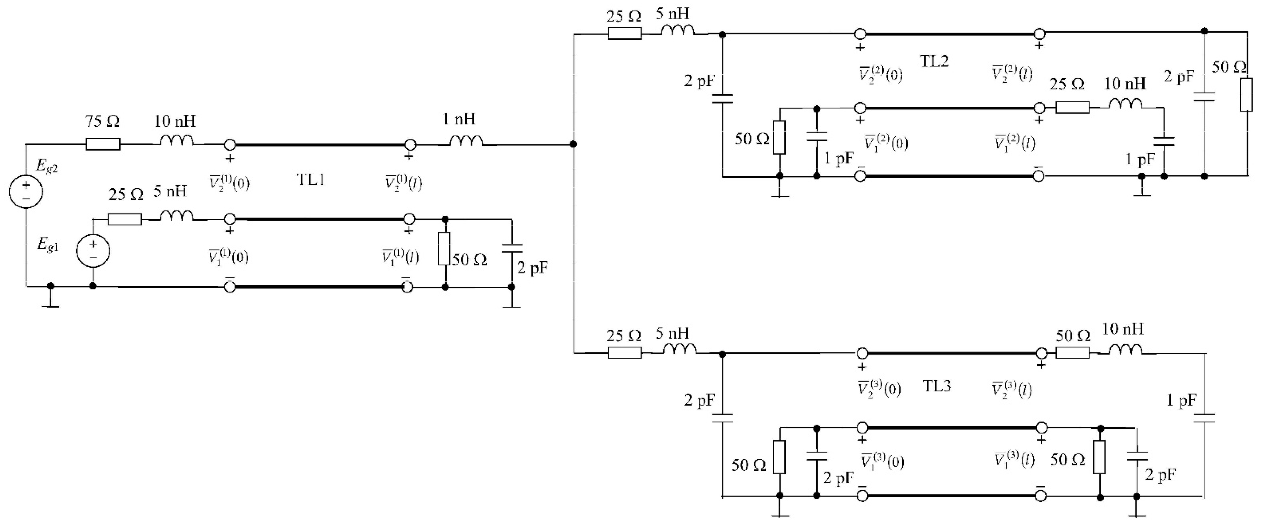
6.3. Example 3

Let us consider the circuit shown in Figure 6, including three DPMTLs. The values of the lumped elements existing in the circuit are indicated in the figure, whereas the p-u-l parameters of the DPMTLs are the same as in Example 1. The length of the lines are as follows: 0.5 m, 0.4 m, and 0.6 m, the amplitudes of the power supply voltage sources are E_g1 = 5 V and E_g2 = 10 V, and the phases are equal to $0^{\mathrm{o}}$, $f$ = 100 MHz. The accuracy of measurement of the voltage amplitudes is 0.1 mV and of the phases is ${0.01}^{\mathrm{o}}$. The end values of $R_S$ are equal to $R_S^{-}=1\mathsf{\Omega }$, $R_S^{+}=1000\mathsf{\Omega }$, the convergence tolerances are $\tilde{\epsilon }=0.001$, ${\tilde{\tilde{\epsilon }}}_1=0.01$, and $\tilde{\tilde{\epsilon }}=0.02$, and the maximum number of iterations $M_{\mathrm{it}}=30$.

To illustrate the proposed method, 12 soft short faults occurring in the DPMTLs, presented in

Table 3. Outcomes of the soft shorts diagnoses in the circuit of Figure 5.

Number of the Fault	The Pair of Conductors Where the Actual Fault Occurs	Actual Value of ${\mathit{R}}_{\mathit{S}}$ (Ω)	Actual Value of $\widehat{\mathit{l}}$ (Ω)	Value of ${\mathit{R}}_{\mathit{S}}$ Given by the Method (Ω)	Value of $\widehat{\mathit{l}}$ Given by the Method (m)	Existence of Virtual Faults
1	0–1 (TL1)	20	0.15	20.00	0.1500	no
2	0–1 (TL1)	150	0.40	150.20	0.3999	no
3	0–2 (TL1)	750	0.20	749.39	0.1994	no
4	0–1 (TL2)	2	0.08	1.99	0.0801	no
5	0–2 (TL2)	50	0.36	49.83	0.3603	no
6	0–2 (TL2)	500	0.28	498.29	0.2797	no
7	0–1 (TL3)	300	0.42	309.13	0.4019	no
8	0–1 (TL3)	920	0.15	934.69	0.1514	no
9	0–2 (TL3)	5	0.21	5.00	0.2099	no
10	1–2 (TL1)	20	0.35	20.02	0.3495	no
11	1–2 (TL2)	500	0.28	505.12	0.2792	yes
12	1–2 (TL3)	680	0.45	688.75	0.4498	yes

, were diagnosed. For each of faults 1–10, the diagnostic method finds only the actual fault. For fault 11, the method finds the actual fault placed in Table 3 and the virtual one, occurring between the conductors 0 and 2 in TL2: $R_S=556.62\mathsf{\Omega }$ $\widehat{l}=0.2788\mathrm{m}$. In addition, for fault 12, the method gives the actual fault and the virtual one, which occurs between the conductors 0 and 2 in TL3: $R_S=772.79\mathsf{\Omega }$, $\widehat{l}=0.4534\mathrm{m}$. The CPU time of each diagnosis including the application of the numerical method described in Section 4 to all possible faults occurring between any pair of the conductors in all the three lines does not exceed 0.55 s.

6.4. Example 4

To illustrate the effectiveness of the method adapted to open fault diagnosis, we consider the circuits of Figure 4, Figure 5 and Figure 6 again. Diagnoses of 45 open faults were carried out numerically: 10 in the circuit of Figure 4, 17 in the circuit of Figure 5, and 18 in the circuit shown in Figure 6 with the same measurement accuracy and convergence tolerances as in Examples 1–3. In all the cases, the method correctly identified the faulty conductor and estimated the fault location $\widehat{l}$. The CPU time in each case including the diagnoses of possible faults in n conductors of all the lines was less than 0.2 s in the circuit of Figure 4, 0.4 s in the circuit of Figure 5, and 0.3 s in the circuit of Figure 6. Outcomes of the diagnoses of 20 open faults are presented in

Table 4. Results of open faults diagnoses in the circuits of Figure 4 and Figure 5.

-	Circuit of Figure 4 $\mathit{l}=0.4\mathbf{m}$			Circuit of Figure 5 $\mathit{l}=0.5\mathbf{m}$
Faulty conductor	1	2	2	1	1	2	2	3	3	4	4
Fault location $\widehat{l}$ (m)	0.060	0.120	0.360	0.150	0.300	0.075	0.400	0.150	0.300	0.150	0.400
$\widehat{l}$ (m) given by the method	0.060	0.120	0.360	0.149	0.298	0.073	0.386	0.150	0.297	0.150	0.396

and

Table 5. Results of open faults diagnoses in the circuit shown in Figure 6.

-	TL1 $\mathit{l}=0.5\mathbf{m}$			TL2 $\mathit{l}=0.4\mathbf{m}$			TL3 $\mathit{l}=0.6\mathbf{m}$
Faulty conductor	1	1	2	1	2	2	1	1	2
Fault location $\widehat{l}$ (m)	0.150	0.475	0.050	0.120	0.015	0.270	0.200	0.400	0.100
$\widehat{l}$ (m) given by the method	0.150	0.475	0.050	0.120	0.015	0.270	0.198	0.395	0.100

.

7. Discussion and Comparisons

This paper deals with very high-frequency electronic circuits, including multiconductor distributed parameter transmission lines and is aimed at the diagnosis of soft short and open faults in the lines. According to our knowledge, this is the first work in that area. However, short fault location and classification in power transmission lines is a significant importance problem that has been a subject of interest to engineers and researchers over the last decades. Therefore, we compare, in the sequel, the diagnostic method proposed in this paper and the methods and techniques for the fault diagnosis of power systems.

In electronic circuits, the transmission line is supplied with a single or several sources of very high frequency, but they do not form a three-phase system as in power transmission lines. As a rule, the circuits include active elements that are modeled using different types of controlled sources and passive elements. In consequence, the standard node method may not hold, which makes it impossible to obtain the impedance matrix [29,32] having the required properties, which is the basis of many fault location methods in power transmission lines.

In multiconductor lines, all kind of couplings play an important role, and none of the p–u–l parameters can be neglected. The proposed method covers all aspects of the short diagnosis: identification of the pair of the conductors where the fault occurs, location of the fault, and estimation of its value. It is also able to detect and locate an open fault. The fault diagnosis of power transmission lines concentrates on the location and classification of shorts, e.g., [29,30,31,32,33,34].

The method presented in this paper constitutes a basis for the fault diagnosis of some class of nonlinear electronic circuits containing multiconductor transmission lines, using the small-signal models of the circuits at the operating point.

Unlike the very high frequency, low voltage electronic circuits, the power systems are the low frequency, high voltage ones. The main diagnostic problem in a power transmission line is the location of short faults. The typical power system includes a three-phase transmission line to deliver power from a power plant to end users. The power systems also include transformers, current transformers, protection relays, and some measurement instruments. In consequence, the diagnostic methods can use phasor data of voltages and currents, e.g., [33,34], whereas in the electronic circuits, the measurement of currents is inconvenient, and the data are limited to voltages. The theory of power circuits is well established, and there are many methods for their analysis, including the methods of finding the impedance matrix commonly used in the fault diagnosis [29]. Impedance-based methods belong to the class of major short fault location methods. In addition, some techniques, such as Clarke and Karrenbauer transformations, enabling decoupling three-phase quantities into other components, are applied to fault detection and location [30]. Most of the works devoted to the short fault diagnosis of power transmission lines relate to the lines modeled by lumped elements. In some works, three-phase distributed parameter transmission lines are represented by three one-phase models using the positive, negative, and zero sequence networks, which considerably simplifies the diagnosis. The fault diagnosis of power transmission lines mainly concentrates on short faults, because they occur much more frequently than the open faults.

Thus, the methods for fault diagnosis of power systems exploit and take advantage of specific properties of this class of circuits and peculiar methods of their analysis. Although there are some features in common, they use the research tools that are not applicable to the fault diagnosis of the electronic circuits.

8. Conclusions

The paper is focused on the diagnosis of soft short and open faults that can occur in a DPMTL terminated by lumped electronic circuits of very high frequency. The method devoted to soft short faults is described in detail. It encompasses all aspects of the diagnosis: identification of the pair of the conductors where the fault occurs, location of the fault, and estimation of its value. The idea of the method can be directly adapted to the soft open fault diagnosis. Unfortunately, unlike the soft short fault case, estimation of the faulty resistor value is possible only if measurement accuracy, while running the diagnostic test, is very high and cannot be assured in real circumstances. However, when the method is applied to open instead of soft open, then it efficiently identifies the conductor where the fault takes place and locates it along this conductor.

The numerical method for solving nonlinear diagnostic equations takes advantage of the particular form of these equations. It is easy to implement, efficient, and very fast. In consequence, the time consumed by the diagnostic method is short, and the method does not require great computing power. Voltage phasors considered in the course of the diagnostic test are measured at one frequency only. The faults are searched taking into account all possible places where they can occur. Drawbacks of the proposed method are as follows. The method is limited to the diagnosis of a single fault. Sometimes, it finds the actual fault and a virtual one, both having equal rights. Occasionally, the method fails.

References

- Gizopoulos, D. Advances in Electronic Testing: Challenges and Methodologies; Springer: Dordrecht, The Netherlands, 2006. [Google Scholar]
- Kabisatpathy, P.; Barua, A.; Sinha, S. Fault Diagnosis of Analog Integrated Circuits; Springer: Dordrecht, The Netherlands, 2005. [Google Scholar]
- Sun, Y. (Ed.) Test and Diagnosis of Analogue, Mixed-Signal and Rf Integrated Circuits: The System on Chip Approach; IET Digital Library: London, UK, 2008. [Google Scholar]
- Binu, D.; Kariyappa, B.S. A survey on fault diagnosis of analog circuits: Taxonomy and state of the art. Int. J. Electron. Commun. 2017, 73, 68–83. [Google Scholar] [CrossRef]
- Fontana, G.; Luchetta, A.; Manetti, S.; Piccirilli, M.C. An unconditionally sound algorithm for testability analysis in linear time-invariant electrical networks. Int. J. Circ. Theor. Appl. 2016, 44, 1308–1340. [Google Scholar] [CrossRef]
- Fontana, G.; Luchetta, A.; Manetti, S.; Piccirilli, M.C. A fast algorithm for testability analysis of large linear time-invariant networks. IEEE Trans. Circuits Syst. I Regul. Papers 2017, 64, 1564–1575. [Google Scholar] [CrossRef]
- Tang, X.; Xu, A.; Li, R.; Zhu, M.; Dai, J. Simulation-based diagnostic model for automatic testability analysis of analog circuit. IEEE Trans. Comput. Aided Des. Integr. Circuit Syst. 2018, 37, 1483–1493. [Google Scholar] [CrossRef]
- Grasso, F.; Luchetta, A.; Manetti, S.; Piccirilli, M.C. A method for the automatic selection of test frequencies in analog fault diagnosis. IEEE Trans. Instrum. Meas. 2007, 56, 2322–2329. [Google Scholar] [CrossRef]
- Saeedi, S.; Pishgar, S.H.; Eslami, M. Optimum test point selection method for analog fault dictionary techniques. Analog Integr. Circuits Signal Proc. 2019, 100, 167–179. [Google Scholar] [CrossRef]
- Czaja, Z. Selt-testing of analog parts terminated by ADCs based on multiple sampling of time responses. IEEE Trans. Instrum. Meas. 2013, 62, 3160–3167. [Google Scholar] [CrossRef]
- Kladovscikov, L.; Jurgo, M.; Navickas, R. Desing of an oscillation–based BISTS system for active analog integrated filters in 0.18 μm CMOS. Electronics 2019, 8, 813. [Google Scholar] [CrossRef] [Green Version]
- Tadeusiewicz, M.; Hałgas, S. A method for multiple soft fault diagnosis of linear analog circuits. Measurement 2019, 131, 714–722. [Google Scholar] [CrossRef]
- Yang, C. Multiple soft fault diagnosis of analog filter circuit based on genetic algorithm. IEEE Access 2020, 8, 8193–8201. [Google Scholar] [CrossRef]
- Deng, Y.; Liu, N. Soft fault diagnosis in analog circuits based on bispectral models. J. Electron. Test. 2017, 33, 543–557. [Google Scholar] [CrossRef]
- Li, Y.; Zhang, R.; Guo, Y.; Huan, P.; Zhang, M. Nonlinear soft fault diagnosis of analog circuits based on RCCA-SVM. IEEE Access 2020, 8, 60951–60963. [Google Scholar] [CrossRef]
- Tadeusiewicz, M.; Hałgas, S. Diagnosis of soft spot short defects in analog circuits considering the thermal behaviour of the chip. Metrol. Meas. Syst. 2016, 23, 239–250. [Google Scholar] [CrossRef] [Green Version]
- Tadeusiewicz, M.; Hałgas, S. A new approach to multiple soft fault diagnosis of analog BJT and CMOS circuits. IEEE Trans. Instrum. Meas. 2015, 64, 2688–2695. [Google Scholar] [CrossRef]
- Tadeusiewicz, M.; Kuczynski, A.; Halgas, S. Catastrophic fault diagnosis of a certain class of nonlinear analog circuits. Circuits Syst. Signal Process. 2015, 34, 353–375. [Google Scholar] [CrossRef] [Green Version]
- Tadeusiewicz, M.; Hałgas, S. Diagnosis of a soft short and local variations of parameters occurring simultaneously in analog CMOS circuits. Microelectron. Reliab. 2017, 72, 90–97. [Google Scholar] [CrossRef]
- Tadeusiewicz, M.; Hałgas, S. A method for local parametric fault diagnosis of a broad class of analog integrated circuits. IEEE Trans. Instrum. Meas. 2018, 67, 328–337. [Google Scholar] [CrossRef]
- Bindi, M.; Grasso, F.; Luchetta, A.; Manetti, S.; Piccirilli, M.C. Smart monitoring and fault diagnosis of joints in high voltage electrical transmission lines. In Proceedings of the 6th International Conference on Soft Computing & Machine Intelligence, Johannesburg, South Africa, 19–20 November 2019; pp. 40–44. [Google Scholar] [CrossRef] [Green Version]
- Binu, D.; Kariyappa, B.S. RideNN: A new rider optimization algorithm—Based neural network for fault diagnosis in analog circuits. IEEE Trans. Instrum. Meas. 2019, 68, 2–26. [Google Scholar] [CrossRef]
- Jahangiri, M.; Razaghian, F. Fault detection in analogue circuit using hybrid evolutionary algorithm and neural network. Analog Integr. Circuits Signal Proc. 2014, 82, 551–556. [Google Scholar] [CrossRef]
- Long, B.; Li, M.; Wang, H.; Tian, S. Diagnostics of analog circuits based on LS-SVM using time-domain features. Circuits Syst. Signal Process. 2013, 32, 2683–2706. [Google Scholar] [CrossRef]
- Yuan, L.; He, Y.; Huang, J.; Sun, Y. A new neural-network-based fault diagnosis approach for analog circuits by using kurtosis and entropy as a preprocessor. IEEE Trans. Instrum. Meas. 2010, 59, 586–595. [Google Scholar] [CrossRef]
- Han, H.; Wang, H.; Tian, S.; Zhang, N. A new analog circuit fault diagnosis method based on improved Mahalanobis distance. J. Electron. Test. 2013, 29, 95–102. [Google Scholar] [CrossRef]
- Luo, H.; Lu, W.; Wang, Y.; Wang, L.; Zhao, X. A novel approach for analog fault diagnosis based on stochastic signal analysis and improved GHMM. Measurement 2016, 81, 26–35. [Google Scholar] [CrossRef]
- Paul, C.R. Analysis of Multiconductor Transmission Lines, 2nd ed.; IEEE Press; John Wiley & Sons Inc.: New York, NY, USA, 2008. [Google Scholar]
- Saha, M.M.; Izykowski, J.; Rosolowski, E. Fault Location on Power Networks; Springer: New York, NY, USA, 2009. [Google Scholar]
- Chen, K.; Huang, C.; He, J. Fault detection, classification and location for transmission lines and distribution systems: A review of the methods. IET High Volt. 2016, 1, 25–33. [Google Scholar] [CrossRef]
- Dalcastagne, A.L.; Filho, S.N.; Zurn, H.H.; Seara, R. An iterative two–terminal fault–location method based on unsynchronized phasors. IEEE Trans. Power Deliv. 2008, 23, 2318–2329. [Google Scholar] [CrossRef]
- Dobakhshari, A.S.; Ranjbar, A.M. A novel method for fault location of transmission lines by wide–area voltage measurements considering measurement errors. IEEE Trans. Smart Grid. 2015, 6, 874–884. [Google Scholar] [CrossRef]
- Lee, Y.J.; Lin, T.C.; Liu, C.W. Multi-terminal nonhomogeneous transmission line fault location utilizing synchronized data. IEEE Trans. Power Deliv. 2019, 34, 1030–1038. [Google Scholar] [CrossRef]
- Yadav, A.; Swetapadma, A. A single ended directional fault section identifier and fault locator for double circuit transmission lines using combined wavelet and ANN approach. Int. J. Electr. Power Energy Syst. 2015, 69, 27–33. [Google Scholar] [CrossRef]
Figure 1.
An (n + 1)-conductor transmission line.
Figure 2.
Circuit including (n + 1)-conductor transmission line.
Figure 3.
Model of the faulty circuit of Figure 2.
Figure 4.
Electronic circuit including three-conductor transmission line (a) and the OPA 695 model (b).
Figure 5.
Circuit including five-conductor transmission line.
Figure 6.
Circuit including three distributed parameter multiconductor transmission lines (DPMTLs).