Economic Emission Load Dispatch Problem with Valve-Point Loading Using a Novel Quasi-Oppositional-Based Political Optimizer

Abstract

In the present paper, a novel meta-heuristic algorithm, namely quasi-oppositional search-based political optimizer (QOPO), is proposed to solve a non-convex single and bi-objective economic and emission load dispatch problem (EELDP). In the proposed QOPO technique, an opposite estimate candidate solution is performed simultaneously on each candidate solution of the political optimizer to find a better solution of EELDP. In the bi-objective EELDP, QOPSO is applied to simultaneously minimize fuel costs and emissions by considering various constraints such as the valve-point loading effect (VPLE) and generator limits for a generation. The effectiveness of the proposed QOPO technique has been applied on three units, six units, 10-units, 11-units, 13-units, and 40-unit systems by considering the VPLE, transmission line losses, and generator limits. The results obtained using the proposed QOPO are compared with those obtained by other techniques reported in the literature. The relative results divulge that the proposed QOPO technique has a good exploration and exploitation capability to determine the optimal global solution compared to the other methods provided in the literature without violation of any constraints and bounded limits.

1. Introduction

With the growing demand for power day by day, the cost incurred in generating power, particularly in fossil fuel plants, is very high. Therefore, it is becoming mandatory to dispatch the power economically to decrease the fuel cost and maintain the stable operation of the power system [1,2]. Thus, the objective of the economic load dispatch problem (ELDP) is to schedule the committed power generating units output to meet the required load demand at minimum fuel cost and satisfy all the system and generating unit constraints. In literature, several conventional techniques such as Newton−Raphson, lambda iteration, dynamic programming, and gradient methods have been recommended to solve this problem. However, as mentioned in [3], the gradient technique has a sluggish convergence rate and has difficulties dealing with inequality restrictions.

Further, the convergence properties of Newton’s technique are sensitive to the initial estimate and may fail to produce an optimal solution owing to incorrect initialization. Inaccuracy and piece-wise linear cost approximation plague the linear programming approach. Furthermore, as mentioned in [3], quadratic programming is inefficient in dealing with the piece-wise quadratic cost approximation. Even though the interior point approach is said to be more efficient computationally, in the case of non-linear objective functions, it may offer an infeasible solution due to improper selection of the step size [4]. Moreover, these conventional techniques require incremental fuel cost curves, which are monotonously increasing/piece-wise linear in nature. However, the input−output characteristics of ELDP are non-convex, non-linear, and nonsmooth in nature [5]. To overcome the drawbacks of conventional techniques, various soft computing methods have been suggested in the literature.

In [5], a fuzzy particle swarm optimization (PSO) is discussed by providing a new mechanism that adjusts the inertia weights of PSO to avoid the premature convergence problem of conventional PSO. An improved firefly algorithm (FA) that prevents the premature convergence problem of standard FA and to enhance the exploration capability is suggested in [6]. A modified flower pollination technique has been suggested by improving the search direction utilizing the user-controlled mutation strategy in the local pollination phase and by carrying an exhaustive exploitation phase to solve ELDP by considering the valve-point effect [7]. In [8], a Q-learning-based PSO is suggested to overcome the drawback of conventional PSO by finding the best policy for exploiting the expected values. A multi-objective PSO is presented in [9] to solve the ELDP problem by minimizing the generation cost and transmission loss as two objective functions. A modified PSO technique has been suggested by making the best use of adaptive acceleration constant in [10]. Here, the acceleration constant best value is selected based on the optimum number of fitness evaluations. In [11], a hybrid bacteria foraging (BFA) and PSO is suggested to solve ELDP by considering the valve-point effect. In this hybrid technique, the best particle’s biased velocity vector is added by BFA random velocity to decrease the randomness during the search process and to increase the swarming. An invasive weed optimization technique is discussed to solve ELDP by considering prohibited operating zones and valve-point effects in [12]. A grey wolf optimizer (GWO)-based ELDP is discussed by application for small to large systems in [13].

Similarly, an ant lion optimization is suggested to solve ELDP by applying it to four small test systems and considering valve-point loading [14]. In [15], a new hybrid method that combines the PSO and pattern search (PS) method has been suggested to solve ELDP. The main objective of this paper is to overcome the disadvantage of the PS method that requires an initial starting point. The authors in [16] have hybridized Big Bang–Big Crunch (BB-BC) and PSO optimization techniques to solve ELDP to enhance the performance and robustness of the conventional BB-BC technique. In [17], an application of artificial bee colony (ABC) optimization to solve ELDP has been discussed by applying it to unit-3, unit-13, and unit-40 test systems with valve-point effect. An application of hybrid differential evolution (DE) and genetic algorithm (GA) with a dynamically coordinated PS algorithm is discussed to improve the solution of the ELDP by considering valve-point loading in [18]. Similar to [13] and [14], the authors in [19] combined the catfish effects on the PSO algorithm to solve ELDP by considering valve-point effects. In [20], the authors considered the traditional ELDP by solving it in a new approach by turning off the inefficient generators by making use of the DE technique. This approach has reduced the total fuel cost by 19.88% when compared to traditional methods. In [21], a relative study of five soft computing techniques, namely, DE, PSO, evolutionary programming (EP), GA, and simulated annealing (SA), is suggested to dynamic ELDP by taking into consideration the constraints such as generator ramp rate limits. In [22], the authors have improved the exploration and convergence capability of conventional teaching learner-based optimization technique by introducing the concept of quasi-oppositional-based learning to solve ELDP. A modified DE technique is suggested to solve ELDP by introducing a tournament-best vector in the mutation stage rather than selecting a random vector, and the random scaling factor is considered instead of a fixed scaling factor to enhance the exploration capability in [23]. In [24], the sequential quadratic programming (SQP) technique is hybridized with PSO to solve ELDP by considering large-scale systems. In a similar way, the authors in [25] have suggested solving ELDP by introducing the self-adaptive chaos and Kalman filtering technique with PSO to circumvent the premature convergence of conventional PSO. In [2], a new evolutionary technique, namely clustering cuckoo search algorithm, is discussed to solve the ELDP by applying it on five different test systems, namely, 6 unit, 10 unit, 11 unit, 13 unit, 15 unit, and 40 unit systems by considering the constraints such as transmission losses and valve-point loading.

It can be observed from the above literature that most of the algorithms [5,6,7,8,9,10,11,12,13,14,15,16,17,18,19,20,21,22,23,24,25] require tuning of a large number of control parameters. Thus, to obtain an optimum solution, the control parameters need to be tuned correctly, which is time-consuming and tedious task. Recently, a human-inspired algorithm, namely political optimizer (PO), has been proposed in [26]. The PO technique mimics the behavior of the politicians, which mathematically maps all the important stages of politics to accomplish the end goal of the optimization. It is observed in [26] that with the tuning of only one control parameter, this technique has shown good convergence speed and exploitation capabilities in solving various engineering design problems. However, in the traditional PO, during its final iterative state of optimization, approximately all the individuals are clustered in a compact region around the present optimal individual in the final stage of iterative optimization. As a result, when tackling complicated multimodal global optimization issues, the complete population may converge to the local optimum quickly. Hence, an improved version of PO that enhances the exploration capability is the main goal of global optimization. Therefore, to enhance the exploration and exploitation capability of the political optimizer, the concept of quasi-oppositional learning is incorporated and named the quasi-oppositional political optimizer (QOPO) method. In the present work, the QOPO method is proposed to solve EELDP. Thus, the main contribution of the work is as follows:

• A novel quasi oppositional-based political optimizer is proposed to enhance the exploration capability of the conventional political optimizer.
• After validating the efficacy of the proposed to solve conventional ELD, it is employed to solve the bi-objective optimization problem (economic emission dispatch).
• To explicate the performance of the proposed QOPO, two practical effects of valve-point loading and transmission line losses are simulated.
• The competence and effectiveness of the proposed QOPO in terms of robustness, quality of the solution, and computational efficiency are compared with various methods suggested in the literature.

Further, the algorithm is tested on different test systems to test the efficiency and robustness, namely, unit 3, unit 6, unit 10, unit 11, unit 13, and unit 40. The rest of the paper is structured in the following way. Section 2 provides the problem formulation of ELDP. The solution methodology is discussed in Section 3. Results and discussions are discussed in Section 4. Finally, conclusions are discussed in Section 4.

2. Formulation of Economic Emission Load Dispatch Problem

The EELDP is a constraint optimization problem that minimizes the total fuel cost and total emission cost that occurred during allocating total power to different generating units. In EELDP, some of the constraints include power balance considering with and without transmission line losses, generating capacity limit, and the effect of valve-point loading [22].

2.1. Objective Function

The objective function of EELDP is to minimize the total fuel cost and minimize the amount of emissions emitted by the generating stations. Thus, the objective function is expressed as the weighted summation of the fuel cost incurred by individual committed generating units and emissions caused by fossil-fuelled thermal units, which is shown below:

$$\min F={\displaystyle \sum _{i=1}^N{C}_i(P_i)}+\sigma \times {\displaystyle \sum _{i=1}^N{E}_i(P_i)}$$

(1)

where C_i(P_i) is the fuel cost obtained by the ith generating unit, E_i(P_i) is the emissions obtained by the ith generating unit, P_i indicates the active power generated by ith generating unit, $\sigma$ indicates the ratio of $C(P_i^{\max })$ and $E(P_i^{\min })$, and N represents the number of generating units.

2.1.1. Smooth Cost Function Characteristics

In standard ELDP, the smooth fuel cost characteristic function is expressed as a quadratic function, described below [22].

$${\displaystyle \sum _{i=1}^N{C}_i(P_i)}={\displaystyle \sum _{i=1}^N{a}_i+b_i{P}_i+c_i{P}_i^2}$$

(2)

where a_i, b_i, and c_i signify the fuel cost coefficients of the ith unit.

2.1.2. Nonsmooth Cost Function Characteristics

In thermal-generating power plants, to control the generating unit’s output power, multiple valves are utilized. The main function of these valves is to control the flow of inlet steam. Thus, these steam valves are opened during the increase in power demand; during this process, a sudden increase in losses is observed, resulting in ripples in the cost curve characteristics. This occurrence is called a valve-point loading effect. This valve-point loading effect accounts for multiple non-differential points and nonsmooth cost curve characteristics [22]. The objective function of ELDP in the presence of valve-point effects makes the conventional objective function as non-convex quadratic, and a sinusoidal function manner as described below:

$${\displaystyle \sum _{i=1}^N{C}_i(P_i)}={\displaystyle \sum _{i=1}^N{a}_i+b_i{P}_i+c_i{P}_i^2}+\left|e_i\sin (f_i(P_i^{\min }-P_i))\right|$$

(3)

where e_i and f_i represent cost coefficients that reflect the valve-point loading effects, and P_i^min indicates the minimum active power generation limit of ith generator.

2.1.3. Nonsmooth Emission Function Characteristics

The emissions caused by fossil fuel generating units are mainly due to two main pollutants, SOx and NOx. The total pollutant emission function is expressed as follows:

$${\displaystyle \sum _{i=1}^N{E}_i(P_i)}={\displaystyle \sum _{i=1}^N{\alpha }_i+{\beta }_i{P}_i+{\gamma }_i{P}_i^2}+{\eta }_i\exp ({\delta }_i{P}_i)$$

(4)

where ${\alpha }_i,{\beta }_i,{\gamma }_i,{\eta }_i,\mathrm{and}{\delta }_i$ represent emission coefficients of ith generator.

From the above equation, it can be observed that the pollutant emission function is very non-linear due to the presence of both quadratic term and exponential function.

2.2. Constraint Functions

2.2.1. Power Balance Constraint

The summation of total power generated by committed generators should be equal to the load demand P_D and the total transmission losses, which is given as follows [22]:

$$\left({\displaystyle \sum _{i=1}^N{P}_i}\right)-P_D-P_L=0$$

(5)

where P_L signifies the total transmission loss.

The losses incurred in transmitting the power from the generation station to load are normally computed using load flow analysis or using Kron’s loss coefficients given below.

$$P_L={\displaystyle \sum _{i=1}^N{\displaystyle \sum _{j=1}^N{P}_i{B}_{ij}{P}_j+{\displaystyle \sum _{i=1}^N{P}_i{B}_{0i}+B_{00}}}}$$

(6)

where B_ij, B_0i, and B₀₀ signify the loss B coefficients and constants during normal operating conditions.

2.2.2. Generation Limit Constraints

The active power-generated output of each generating unit should satisfy the maximum P^max and minimum P^min limits which is expressed as [22]:

$$P_i{}^{min}\le P_i\le P_i{}^{max},fori=1,2,3,\dots ,N.$$

(7)

3. Solution Methodology Using QOPO

The political optimizer is a new meta-heuristic optimization technique proposed in the year 2020 and is based on the multi-phase political process [26]. This PO technique mimics the behavior of the politicians to accomplish the end goal of the optimization. This PO technique is generalized by incorporating few harmonies such as the concept of parties and its participation in various constituencies, the connotation of politicians with the parties, cooperation between the politicians within the same party and competition between the other parties through the inter-party election, switching of politicians from one party to the other, confrontation before the election for votes, and cooperation between the members elected during the election in parliament [26]. Thus, PO performs five sequences of phases to optimize the given problem, which are (1) party creation and allocation of the constituency, (2) campaigning during election, (3) party switching, (4) election between the politicians of the inter-party, and (5) parliamentary affairs.

3.1. Party Creation and Allocation of Constituency

Like all other meta-heuristic techniques, the algorithm starts with initializing the population P of size NP. Here, each row in the population constitutes the political party and the number of constituencies [26]. The number of input variables of the problem is denoted as D.

$$P=\{P_{i,1},P_{i,2},\dots P_{i,D}\},i=1,2,\dots NP$$

(8)

Further, in addition, as a party member, a political solution acts as an election candidate. This is shown as follows:

$$\begin{array}{l}C=\{C_1,C_2,\dots C_n)\\ C_j=\{P_i^j,P_2^j,\dots P_n^j\}\end{array}$$

(9)

From the above, it can be considered as there are “n” numbers of constituencies in which “n” number of parties compete in each constituency C.

The best member of the party based on fitness is considered as the leader of the party. The selection of the leader of the party is exhibited as follows [26]:

$$\begin{array}{c}q=ar\min f(P_i^j),\forall i\in \{1,2,3,\dots n\}and1\le j\le n\\ P_i^{*}=P_i^q\end{array}$$

(10)

where $P^{*}=\{P_1^{*},P_2^{*},\dots ,P_n^{*}\}$ represents the set of all the political party leaders.

If $C_i^{*}$ represents the candidate won from constituency i, then the set of winning candidates form the parliamentarians C^*, which is given as follows:

$$C^{*}=\{C_1^{*},C_2^{*},\dots ,C_n^{*}\}$$

(11)

3.2. Election Campaigning

In this phase, each candidate improves its majority by considering aspects, namely, (1) candidates learning from their previous election, (2) influencing the voters with reference to the leader of the party and by himself, and (3) by performing the comparative analysis with the constituency winner. The campaigning of the candidate follows these three stages and updates his position either using (12) or (13) based on its relation with the previous position, i.e., if the fitness of the candidate is improved, then the position is updated using (12); otherwise, it is updated using (13) [26]. These are explained using the following two equations:

$$p_{i,k}^j(t+1)=\{\begin{array}{ll}{m}^{*}+rand·(m*-p_{i,k}^j(t)),& if{p}_{i,k}^j(t-1)\le p_{i,k}^j(t)\le m^{*}\mathrm{or}{p}_{i,k}^j(t-1)\ge p_{i,k}^j(t)\ge m^{*}\\ m^{*}+(2\times rand-1)·\left|m*-p_{i,k}^j(t)\right|,& if{p}_{i,k}^j(t-1)\le m^{*}\le p_{i,k}^j(t)\mathrm{or}{p}_{i,k}^j(t-1)\ge m^{*}\ge p_{i,k}^j(t)\\ m^{*}+(2\times rand-1)·\left|m*-p_{i,k}^j(t-1)\right|,& if{m}^{*}\le p_{i,k}^j(t-1)\le p_{i,k}^j(t)\mathrm{or}{m}^{*}\ge p_{i,k}^j(t-1)\ge p_{i,k}^j(t)\end{array}$$

(12)

$$p_{i,k}^j(t+1)=\{\begin{array}{ll}{m}^{*}+(2\times rand-1)·\left|m*-p_{i,k}^j(t)\right|,& if{p}_{i,k}^j(t-1)\le p_{i,k}^j(t)\le m^{*}\mathrm{or}{p}_{i,k}^j(t-1)\ge p_{i,k}^j(t)\ge m^{*}\\ p_{i,k}^j(t-1)+rand(p_{i,k}^j(t)-p_{i,k}^j(t-1)),& if{p}_{i,k}^j(t-1)\le m^{*}\le p_{i,k}^j(t)\mathrm{or}{p}_{i,k}^j(t-1)\ge m^{*}\ge p_{i,k}^j(t)\\ m^{*}+(2\times rand-1)·\left|m*-p_{i,k}^j(t-1)\right|,& if{m}^{*}\le p_{i,k}^j(t-1)\le p_{i,k}^j(t)\mathrm{or}{m}^{*}\ge p_{i,k}^j(t-1)\ge p_{i,k}^j(t)\end{array}$$

(13)

3.3. Party Switching

In this phase, a member of the party $P_i^j$ is selected based on the adaptive parameter $\lambda$ and switched to the other party $P_r$ having the least fit member $P_r^q$ randomly [26]. The index q is computed using (14).

$$q=\arg \max f(p_r^j),1\le j\le n$$

(14)

3.4. Election Phase

In this phase, a candidate is said to win the election based on fitness and is represented by (17).

$$\begin{array}{c}q=\arg \min f(p_r^j),1\le j\le n\\ c_j^{*}=p_q^j\end{array}$$

(15)

Here, after the candidate is declared as the winner of a constituency, the party leaders are updated using (10).

3.5. Parliamentary Affairs

In this stage, the government is formed after the election. The leaders of the party and parliamentarians are categorical by using (10) and (15), respectively. Now, each parliamentarian updates his position by selecting another parliamentarian randomly if there is an improvement in fitness [26]. A detailed explanation of the conventional PO can be found in [26].

3.6. Quasi-Opposition-Based Learning

After performing the parliamentary operation, the fitness of each parliamentarian is examined by quasi-opposition position, i.e., here, the concept of quasi-opposition-based learning (QOBL) is applied to each parliamentarian. Then, after obtaining the fitness of the quasi-opposition position of each parliamentarian, the best NP parliamentarians are selected for the next iteration. To perform the QOBL, the opposite position of the parliamentarian to the present position of the parliamentarian, along with the mean of the search region, is calculated. Here, the opposite position of the parliamentarian to the given position of the parliamentarian and the mean of the search region is calculated in the following way [22].

If $z_i\left(z_{i,1},z_{i,2},\dots ,z_{i,d}\right)$ is a vector comprised of d-real numbers whose upper and lower limits are $z_j=[z_j^{min},z_j^{max}]\forall j\in \{1,2,\dots ,d\}$, then its opposite vector $o{z}_i\left(o{z}_{i,1},o{z}_{i,2},\dots ,o{z}_{i,d}\right)$ is obtained using (16).

$$o{z}_j=z_j^{min}+z_j^{max}-z_j$$

(16)

The mean (mz) of the search space limit is calculated as:

$$mz=\frac{\left(z_j^{min}+z_j^{max}\right)}{2}$$

(17)

Mathematically, the QOBL is obtained using (18):

$$QO{Z}_j=rand\left(\frac{z_j^{min}+z_j^{max}}{2},z_j^{min}+z_j^{max}-z_j\right)$$

(18)

Now, each position of the parliamentarian obtained after the parliamentarian phase is compared with the QOZ position of the parliamentarian obtained above to select the best individual for next-generation or iteration.

The step-by-step implementation of the proposed QOPO to EELD problem is shown in Figure 1.

4. Results and Discussion

To illustrate the efficiency of the proposed QOPO algorithm to solve EELDP, it is initially tested by pertaining it to solve conventional ELDP, i.e., minimizing fuel cost by considering three real-world benchmark test systems. This is as follows: case study 1 deals with the small test system that consists of three generating units with 850 MW load demand. Case study 2 deals with the medium test system that consists of 13 generating units with 1080 MW and 2520 MW load demands. Case study 3 deals with the large-scale test system that consists of 40 generating units with 10,500 MW load demand. After verifying the ability to solve conventional ELDP, the proposed method is applied to solve bi-objective functions, i.e., minimizing the total fuel cost and the total emission by considering valve-point loading effect, generator limits, and transmission line losses on unit 6, unit 10, unit 11, and unit 40 systems. For all the experiments, the proposed QOPO technique has been executed with a population size of 64 (the number of parties (8) multiplied by the number of constituencies (8)) and a lambda value of 0.2. These control parameters have been selected by varying the population size, i.e., {25, 36, 49, 64, 81, 100} and lambda value from 0.05 to 0.4 with variation of 0.05. Further, the maximum number of iterations taken for unit 3, unit 6, unit 10, unit 11, unit 13, and unit 40 are 500, 1500, 5000, 5000, 5000, and 10,000, respectively.

4.1. Single Objective Function (Minimizing the Total Fuel Costs)

4.1.1. Case Study 1: Three Generating Units with 850 MW Load Demand

In this case study, the three-unit generating system is utilized to evaluate the performance of the proposed QOPO with a load demand of 850 MW by considering the valve-point loading effect. The fuel cost coefficients and generator maximum and minimum limits have been taken from [8,27]. The results obtained using QOPO are provided in

Table 1. Comparison of power distribution among three units for the load demand of 850 MW.

Method	P1 (MW)	P2 (MW)	P3 (MW)	PG (MW)	Cost (USD/h)
GA [28]	398.7	399.6	50.1	848.4	8222.1
EP [28]	300.3	400	149.7	850	8234.1
EP-SQP [28]	300.3	400	149.7	850	8234.1
PSO [28]	300.3	400	149.7	850	8234.1
PSO-SQP [28]	300.3	400	149.7	850	8234.1
PS [28]	300.3	399.9	149.7	850	8234.1
GA-PS-SQP [28]	300.3	400	149.7	850	8234.1
GSA [29]	300.2102	149.7953	399.9958	850.0013	8234.1
Proposed QOPSO	300.25	400	149.75	850	8234.07

, along with the results obtained in the literature. Table 1 represents the power allocation between different generators for a given load demand of 850 MW. It is seen that the proposed QOPO gives better results (with a total cost of 8234.07 USD/h) when compared to GA, EP, EP-SQP, PSO, PSO-SQP, PS, GA-PS-SQP, gravitational search algorithm (GSA) techniques. Further, the results are summarized in

Table 2. Comparison of results of 3-unit system for the load demand of 850 MW.

Method	Minimum Cost (USD/h)
GAB [27]	8234.08
MFEP [27]	8234.08
GA-PS-SQP [28]	8234.10
GWO [13]	8253.11
GSA [29]	8234.1
HCPSO [30]	8234.07
HCPSO-SQP [30]	8234.07
iBA [31]	8234.07
NDS [32]	8234.07
NSS [33]	8234.08
SA [33]	8234.1355
GA [33]	8234.4190
EP [33]	8234.1357
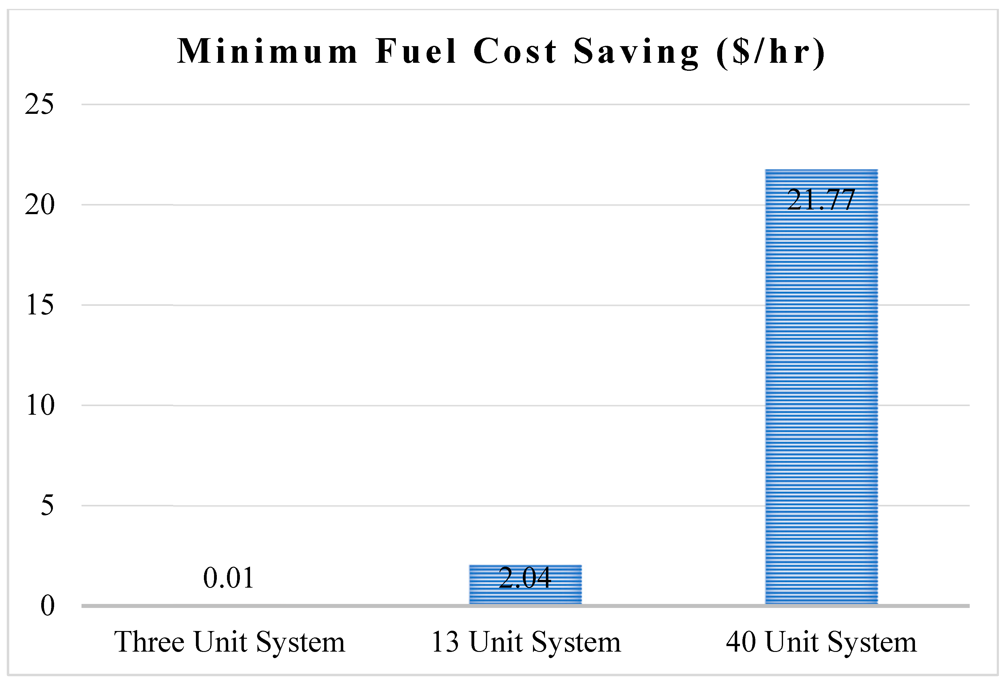
Proposed QOPO	8234.07

and compared with other comparative techniques suggested in the literature. The proposed method being tested on a small test system, the results obtained using proposed method is similar to few techniques (island bat algorithm (iBA), Hybrid Chaotic PSO (HCPSO), HCPSO-SQP). However, still being a small sized test system, the proposed method has been able to provide better results than other techniques such as GAB, mean fast EP (MFEP), GA-PS-SQP, GWO, GSA, novel direct search method (NDS), novel stochastic search method (NSS), SA, EP, and GA. When compared with these techniques, there is a minimum saving of 0.01 USD/h and maximum saving of 19.04 USD/h when compared to GAB and GWO techniques, respectively.

4.1.2. Case Study 2: 13 Generating Units System with 1080 MW and 2520 MW Load Demands

In this case study, the 13 generating unit system is utilized to evaluate the performance of the proposed QOPO with load demands of 1080 MW and 2520 MW by considering the valve-point loading effect. The fuel cost coefficients and generator maximum and minimum limits have been taken from [8,27]. The results obtained using QOPO are provided in

Table 3. Comparison of power distribution among 13 units for the load demand of 1800 MW.

Unit	NN-EPSO [13]	GWO [13]	Proposed QOPO
P1	490	807.1247	628.3183
P2	189	144.869	298.1864
P3	214	297.9434	223.7622
P4	160	60	60.00008
P5	90	60	60
P6	120	60	60
P7	103	60	159.7331
P8	88	60	60
P9	104	60.0362	60
P10	13	40	40
P11	58	40.0267	40
P12	66	55	55
P13	55	55	55.00001
TG (MW)	1750	1800	1800
Total Cost (USD/h)	18,442.59	18,051.11	17,988.99

and

Table 4. Comparison of results of 13-unit system for the load demand of 1800 MW.

Method	Minimum Cost (USD/h)
CEP [27]	18,048.21
FEP [27]	18,018.00
MFEP [27]	18,028.09
IFEP [27]	17,994.07
PSO [34]	18,030.72
EP-SQP [34]	17,991.03
Proposed QOPO	17,988.99

for 1080 MW and 2520 MW load demands, along with the results obtained in the literature. Table 3 and

Table 5. Comparison of power distribution among 13 units for the load demand of 2520 MW.

Unit	GA [34]	SA [34]	Proposed QOPO
P1	628.32	668.4	628.3147
P2	356.49	359.78	359.9905
P3	359.43	358.2	359.3237
P4	159.73	104.28	109.8603
P5	109.86	60.36	159.7333
P6	159.73	110.64	159.7275
P7	159.63	162.12	159.6924
P8	159.73	163.03	159.7204
P9	159.73	161.52	159.6847
P10	77.31	117.09	40.00002
P11	75	75	113.952
P12	60	60	55.00017
P13	55	119.58	55.00017
TG (MW)	2519.96	2520	2520
Total Cost (USD/h)	24,398.23	24,970.91	24,328.14

represent the power allocation between different generators for given load demands of 1080 MW and 2520 MW, respectively. It is seen that the proposed QOPO gives better results (with a total cost of 17,988.99 USD/h and 24,328.14 USD/h, respectively) when compared to neural network (NN)-efficient PSO (NN-EPSO), GWO, SA, and GA techniques. Further, the results are summarized in Table 5 and

Table 6. Comparison of results of 13-unit system for the load demand of 2520 MW.

Method	Minimum Cost (USD/h)
SA [34]	24,970.91
GA [34]	24,398.23
Proposed QOPO	24,328.14

for 1080 MW and 2520 MW load demands, respectively. These summarized results are compared with other comparative techniques suggested in the literature. It is observed from Table 3, Table 4, Table 5 and Table 6 that the proposed method is able to provide better results than other techniques such as classical EP (CEP), Fast EP (FEP), MFEP, improved FEP (IFEP), PSO, EP-SQP, SA, and GA. As the size of the system has been increased to 13 units, the proposed method has been able to save a minimum of 2.04 USD/h and a maximum of 453.6 USD/h when compared to EP-SQP and NN-EPSO methods, respectively, for load demand of 1800 MW. It has also been observed that with increase in demand to 2520 MW from 1800 MW, there is further saving with a minimum of 70.09 USD/h and maximum of 642.77 USD/h in comparison with GA and SA, respectively. This shows the efficiency of the proposed QOPO technique.

4.1.3. Case Study 3: 40 Generating Units System with 10,500 MW Load Demand

In this case study, the 40 generating unit system is utilized to evaluate the performance of the proposed QOPO with a load demand of 10,500 MW by considering the valve-point loading effect. The fuel cost coefficients and generator maximum and minimum limits have been taken from [8,27]. The results obtained using QOPO are provided in

Table 7. Comparison of power distribution among 40 units for the load demand of 10,500 MW.

Unit	MPSO [35]	PSO [36]	MPPSO [36]	APPSO [36]	DPSO [36]	Proposed QOPO
P1	114	113.116	112.903	112.579	111.917	113.7611
P2	114	113.01	112.802	111.553	112.338	113.9886
P3	120	119.702	117.515	98.751	118.922	119.9993
P4	182.222	81.647	181.442	180.384	179.928	189.8949
P5	97	95.062	95.876	94.389	48.998	97
P6	140	139.209	139.856	139.943	139.931	139.9986
P7	300	299.127	299.452	298.937	299.61	300
P8	299.021	287.491	298.277	285.827	298.206	299.9992
P9	300	292.316	299.043	298.381	285.372	299.997
P10	130	279.273	130.886	130.212	130.701	130
P11	94	169.766	243.53	94.385	94.849	94.00011
P12	94	94.344	94.768	169.583	244.086	94.35996
P13	125	214.871	215.033	214.617	214.739	125.1963
P14	304.485	304.79	304.739	304.886	304.504	304.5059
P15	394.607	304.563	304.694	304.547	304.744	394.4782
P16	305.323	304.302	215.146	304.584	304.501	394.2599
P17	490.272	489.173	497.407	489.452	489.515	489.331
P18	500	491.336	489.459	497.472	489.534	489.4125
P19	511.404	510.88	511.867	512.816	511.567	511.2939
P20	512.174	511.474	548.4	548.992	511.374	511.4796
P21	550	524.814	523.396	524.652	525.246	525.461
P22	523.655	524.775	525.206	523.399	523.979	523.6933
P23	534.661	525.563	524.971	548.895	548.599	526.5896
P24	550	522.712	523.66	525.871	523.314	524.3047
P25	525.057	503.211	523.624	523.814	523.259	524.7312
P26	549.155	524.199	527.932	523.565	524.36	523.5606
P27	10	10.082	10.474	10.575	10.388	10
P28	10	10.663	11.074	11.177	10.552	10.22341
P29	10	10.418	10.582	11.21	10.082	10.08921
P30	97	94.244	96.403	96.178	96.422	97
P31	190	189.377	189.338	189.999	189.692	190
P32	190	189.796	189.849	189.924	189.82	189.9998
P33	190	189.813	189.739	189.714	189.954	190
P34	200	199.797	199.808	199.284	199.427	200
P35	200	199.284	199.994	199.599	199.905	200
P36	200	198.165	199.749	199.751	199.229	199.9999
P37	110	109.291	109.917	109.973	109.565	109.9804
P38	110	109.087	109.41	109.506	109.741	110
P39	110	109.909	109.728	109.363	109.575	110
P40	512.964	512.348	512.053	511.261	511.554	511.4108
TG (MW)	10,500	10,473	10,500	10,500	10,500	10,500
Total Cost (USD/h)	122,252.265	1,223,243.97	122,225.73	122,044.63	122,159.99	121,789.6

for 10,500 MW load demand, along with the results obtained in the literature. Table 7 represents the power allocation between different generators for a given load demand of 10,500 MW. It is seen that the proposed QOPO gives better results (with a total cost of 121,789.6 USD/h) when compared to modified PSO (MPSO), PSO, mean personal best base-oriented particle PSO (MPPSO), adaptive personal best base-oriented PSO (APPSO), and decisive personal base-oriented PSO (DPSO) techniques. Further, the results are summarized in

Table 8. Comparison of results of 40-unit system for the load demand of 10,500 MW.

Method	Minimum Cost (USD/h)
CEP [27]	123,488.29
FEP [27]	122,679.71
MFEP [27]	122,647.57
IFEP [27]	122,624.35
GA [37]	121,996.40
EP-SQP [34]	122,323.97
PSO [34]	123,930.45
PSO-SQP [34]	122,094.67
MPSO [35]	122,252.27
ESO [38]	122,122.16
TM [39]	122,477.78
TS [40]	122,288.38
ACO [40]	121,811.37
EGA [18]	122,022.96
FIA [18]	121,823.80
PSO [36]	122,323.97
MPPSO [36]	122,225.73
APPSO [36]	122,044.63
DPSO [36]	122,159.99
Proposed QOPO	121,789.6

Notes: Evolutionary structural optimization (ESO), Taguchi method (TM), Tabu search (TS), Ant colony optimization (ACO), Fuzzy self-adaptive immune algorithm (FIA).

for 10,500 MW load demands. These summarized results are compared with 19 other comparative techniques suggested in the literature. The best results obtained for the given test system are represented with bold letters. It has been observed from Table 8 that the proposed method is able to provide a minimum saving of 21.77 USD/h and a maximum saving of 2140.85 USD/h when compared to ACO and PSO techniques, respectively. This shows the robustness of the proposed QOPO technique to provide efficient results. Further, the minimum saving of fuel cost with increase in number of generating units has been depicted in Figure 2.

4.2. Bi-Objective Function (Minimizing the Total Fuel Cost and the Total Emission)

4.2.1. Case Study 1: Six Generating Units with 2.834 (p.u.) Load Demand

In this case study for bi-objective optimization, a small test system with six generating unit system is initially considered to evaluate the execution of the proposed QOPO with load demand 2.834 p.u. by considering the transmission line losses. The fuel cost coefficients, emission coefficients, and generator maximum and minimum limits have been taken from [41,42]. The results obtained using QOPO are provided in

Table 9. Comparison of results of six-unit system for the load demand of 2.834 p.u.

Unit	1	2	3	4	5	6	C (USD/h)	E (ton/h)
SMODE	0.314	0.4169	0.5424	0.5856	0.549	0.4552	624.44	0.1968
NSGA	0.3234	0.3514	0.6307	0.5877	0.46	0.5084	624.97	0.198
MOEA/D	0.3185	0.4101	0.5623	0.5635	0.545	0.4631	625.69	0.1964
NSGA	0.2712	0.367	0.8099	0.755	0.1357	0.5239	625.71	0.2163
NPGA	0.2998	0.4325	0.7342	0.6852	0.156	0.5561	630.06	0.2079
SPEA	0.2752	0.3752	0.5796	0.677	0.5283	0.4282	617.57	0.2001
MOPSO	0.2882	0.3965	0.732	0.752	0.1489	0.5463	626.1	0.2106
MBFA	0.2595	0.3769	0.5636	0.6759	0.5499	0.4344	616.496	0.2002
FSBF	0.261602	0.378998	0.573339	0.687019	0.530804	0.430789	616.1627	0.2005
NSBF	0.279071	0.406301	0.567423	0.683964	0.49532	0.430657	617.9531	0.2
NGPSO	0.3062	0.4042	0.5577	0.5836	0.5495	0.4610	623.8705	0.1970
Proposed QOPO	0.1211	0.2864	0.5835	0.9924	0.5240	0.3520	605.9984	0.2044

Note: C: Fuel Cost and E: Emission.

for 2.834 p.u. load demand, along with the results obtained in the literature [41]. Table 9 represents the power allocation between different generators for a given load. It can be seen that the proposed QOPO gives better results (with a total cost of 605.9984 USD/h and 0.2044 (ton/h)) when compared to other techniques. It is to be noted here that even though the proposed method provides a slightly high emission of 0.008 (ton/h) compared to MOEA/D, the total fuel cost is a lot less at 19.6916 (USD/h). The best results obtained for the given test system are represented with bold letters. Hence, it can be said from Table 9 that the proposed method can provide a better compromised solution of total fuel cost and emission compared to other techniques.

4.2.2. Case Study 2: Six Generating Units with 1200 MW Load Demand

In continuation to case study 1, in this case, again, a small test system has been considered to verify its effectiveness to provide a better and accurate solution for high load demand. The fuel cost coefficients, emission coefficients, and generator maximum and minimum limits have been taken from [41,42]. The results obtained using QOPO for minimizing the objectives are tabulated in

Table 10. Comparison of results of six-unit system for the load demand of 1200 MW.

Unit	1	2	3	4	5	6	C	E
QOTLBO	107.3101	121.497	206.501	206.5826	304.9838	304.6036	64,912	1281
TLBO	107.8651	121.5676	206.1771	205.1879	306.5555	304.1423	64,922	1281
MODE	108.6284	115.9456	206.7969	210	301.8884	308.4127	64,843	1286
PDE	107.3965	122.1418	206.7536	203.7047	308.1045	303.3797	64,920	1281
NSGA	113.1259	116.4488	217.4191	207.9492	304.6641	291.5969	64,962	1281
SPEA	104.1573	122.9807	214.9553	203.1387	316.0302	289.9396	64,884	1285
MOGA	108.9318	123.1808	205.1513	206.67	304.8553	302.6093	64,838.57	1285.49
OGHS	105.7331	119.0825	205.2976	204.7772	305.8042	308.9128	64,722.74	1281.349
NGPSO	144.0425	150	190.507	192.9285	284.9083	288.0456	66,538.34	1228.365
Proposed QOPO	82.83027	82.61994	197.7722	202.2269	317.4203	317.6234	61,197.88	1238.819

Note: C: Fuel Cost and E: Emission.

for load demand of 1200 MW. The obtained results are compared with nine different techniques proposed in the literature and have been taken from [41]. Like case study 1 for six generating units with load demand of 2.3834 p.u., the proposed method provides better fuel cost when compared to other techniques with slightly high emission of (9.5 ton/h) compared to NGPSO. This slightly high emission is obtained due to the high minimization of fuel cost of 61,197.87551 USD/h, which is less by an amount of 5340.46479 USD/h compared to NGPSO. Further, when compared to other techniques, it has been observed that the proposed QOPO provides not only minimum fuel cost but also the minimum emission cost. Therefore, it can be said that the proposed QOPO provides a better compromised solution.

4.2.3. Case Study 3: Ten Generating Units with 2000 MW Load Demand

In this case study, the efficacy of the proposed method in providing a better solution is tested on ten generating units system by considering nonsmooth fuel test function, i.e., the valve-point loading effect along with transmission line losses. The fuel cost coefficients, emission coefficients, and generator maximum and minimum limits have been taken from [41,42]. The results obtained using QOPO have been provided in

Table 11. Comparison of results of 10-unit system for the load demand of 2000 MW.

Unit	BSA	MODE	PDE	NSGA	SPEA 2	GSA	MOGA	QOTLBO	TLBO	FPA	OGHS	NGPSO	Proposed QOPO
1	55	54.9487	54.9853	51.9515	52.9761	54.9992	54.1807	55	55	53.188	55	55	54.99873825
2	80	74.5821	79.3803	67.2584	72.813	79.9586	78.4981	80	80	79.975	79.9998	80	77.55912431
3	86.5308	79.4294	83.9842	73.6879	78.1128	79.4341	84.7653	84.8457	83.9202	78.105	85.2236	81.2398233	77.09181067
4	86.9844	80.6875	86.5942	91.3554	83.6088	85	81.3502	83.4993	82.8342	97.119	84.3022	80.8334296	77.25725491
5	129.1542	136.855	144.439	134.052	137.243	142.106	138.0526	142.921	132.013	152.74	137.124	160	160
6	146.9258	172.639	165.776	174.95	172.919	166.567	166.2667	163.2711	173.988	163.08	155.894	235.008791	240
7	300	283.823	283.212	289.435	287.202	292.875	295.466	299.8066	299.71	258.61	299.998	289.350745	274.301907
8	323.9002	316.341	312.771	314.056	326.402	313.239	326.7642	315.4388	317.968	302.22	315.726	297.45423	276.8507856
9	435.9938	448.592	440.114	455.698	448.881	441.178	428.9338	428.5084	427.017	433.21	434.941	401.507284	380.9511212
10	440.0149	436.429	432.678	431.805	423.903	428.631	429.6309	430.5524	431.396	466.07	436.007	401.427524	381.7419224
C	112,807.373	113,480	113,510	113,540	113,520	113,490	113,422.34	113,460	113,471	113,370	113,140	116,179.649	111,892.4096
E	4188.0926	4124.9	4111.4	4130.2	4109.1	4111.4	4120.5204	4110.2	4113.5	3997.7	4144.41	3939.2278	3653.343267

Note: C: Fuel Cost and E: Emission.

for load demand of 2000 MW. The results have been compared with different techniques provided in [41]. From this table, it can be observed that with the increase in the number of generating units along with the complex objective function, i.e., by considering VPLE, the proposed QOPO method provided better fuel cost compared to other techniques and the emission cost also. For instance, the proposed method has been able to save the fuel cost a minimum of 914.9639 USD/h and a maximum of 4287.239 USD/h in comparison with BSA and NGPSO, respectively. Similarly, emission cost has been reduced by a minimum of 285.8845 ton/h and a maximum of 534.7493 ton/h when compared to NGPSO and BSA techniques, respectively. This shows the robustness of the proposed QOPO method in providing better solutions compared to other techniques.

4.2.4. Case Study 4: Eleven Generating Units with 2500 MW Load Demand

In this case study, the proposed QOPO method is applied to the 11 generating unit system by considering transmission line losses without the VPLE effect. The data for this generating unit has been taken from [41,42] and the results thus obtained are tabulated in

Table 12. Comparison of results of the 11-unit system for the load demand of 2500 MW.

Unit	NGPSO	SRA	GSA	GA-SC	Proposed QOPO
1	243.335	139.672	138.9382	138.8618	149.064269
2	210	112.781	110.2728	112.1312	128.5976932
3	250	145.802	147.9728	146.7169	172.8199607
4	169.0338	221.527	221.1072	222.1041	200.2368173
5	142.6156	136.774	137.7986	137.1962	162.8987867
6	168.8431	218.578	217.9015	217.3208	197.7004668
7	142.5922	140.261	141.3801	140.4711	161.9169099
8	317.2895	345.046	349.6497	348.9008	356.8327481
9	276.5437	329.484	327.3178	326.5188	312.2170295
10	303.2289	363.645	363.4766	363.5275	344.3533839
11	276.5181	346.43	344.1847	346.2508	313.3619348
C	13,025.91	12,424.94	12,422.66	12,423.77	12,491.67857
E	1661.712	2003.3	2002.95	2003.03	1897.861924

Note: C: Fuel Cost and E: Emission.

. The comparative results have been taken from [41]. From the table, it is identified that as the fuel cost is minimized, the emission has been increased, for instance, in the case of GSA technique, i.e., the GSA technique provides a reduced fuel cost of 69.018 USD/h. However, the reduced fuel cost provided by GSA is due to an increased emission cost of 105.088 ton/h in comparison with the proposed QOPO. On the other hand, if the emission is decreased, the total fuel cost has been increased; for example, in the case of NGPSO technique, i.e., NGPSO provides a minimum emission cost of 236.149 ton/h with an increased fuel cost of 534.23143 USD/h when compared to proposed QOPO technique. In this situation, the proposed QOPO technique has provided a better compromised solution of the two objectives with 12,491.67857 USD/h and 1897.861924 ton/h.

4.2.5. Case Study 5: Forty Generating Units with 10,500 MW Load Demand

In this case study, the effectiveness of the proposed method in providing a better solution is tested on a large test system consisting of forty generating units by considering nonsmooth fuel test function, i.e., the valve-point loading effect. The complete details of fuel cost coefficients, emission coefficients, and generator maximum and minimum limits have been taken from [41,42]. The results obtained using QOPO and the comparative results acquired using other techniques that are taken from [41] have been provided in

Table 13. Comparison of results of 40-unit system for the load demand of 10,500 MW.

Unit	SMPSO	PDE	SPEA 2	MODE	QOTLBO	NSGA	FPA	TLBO	NGPSO	MoGA	GSA	Proposed QOPO
1	114	112.1549	113.9694	113.5295	114	113.8685	43.405	114	113.9988	113.476	113.9989	113.9998896
2	114	113.9431	114	114	114	113.6381	113.95	114	114.0000	114	113.9896	113.9993622
3	120	120	119.8719	120	120	120	105.86	91.9893	119.9999	120	119.9995	119.9999631
4	179.7335	180.2647	179.9284	179.8015	179.7593	180.7887	169.65	177.4467	174.2365	179.618	179.7857	172.6450978
5	97	97	97	96.7716	97	97	96.659	97	96.9994	96.776	97	96.99999276
6	140	140	139.2721	139.276	140	140	139.02	140	127.4300	139.35	139.0128	125.7668413
7	300	299.8829	300	300	300	300	273.28	300	300.0000	300	299.9885	299.997095
8	300	300	298.2706	298.9193	298.9093	299.0084	285.17	283.7368	299.5539	298.898	300	298.3122176
9	289.1440	289.8915	290.5228	290.7737	300	288.889	241.96	300	298.0215	290.693	296.2025	297.7050874
10	130.0114	130.5725	131.4832	130.9025	130.0996	131.6132	131.26	130	130.0314	130.796	130.385	130.0000409
11	243.6004	244.1003	244.6704	244.7349	243.7055	246.5128	312.13	318.1965	304.6847	243.823	245.4775	301.5550053
12	243.6164	318.284	317.2003	317.8218	318.4741	318.8748	362.58	241.5727	303.1886	317.351	318.2101	300.9720619
13	394.2810	394.7833	394.7357	395.3846	394.4004	395.7224	346.24	391.9916	429.2040	394.431	394.6257	433.3831706
14	394.2808	394.2187	394.6223	394.4692	394.3418	394.1369	306.06	394.4501	415.0447	394.769	395.2016	419.2396883
15	394.2856	305.9616	304.7271	305.8104	394.2703	305.5781	358.78	394.3549	418.8330	304.514	306.0014	420.5591571
16	394.2831	394.1321	394.7289	394.8229	394.4013	394.6968	260.68	394.0597	417.7762	394.044	395.1005	420.5783426
17	489.2791	489.304	487.9857	487.9872	489.3143	489.4234	415.19	490.5281	443.8465	488.45	489.2569	442.8324736
18	489.2813	489.6419	488.5321	489.1751	489.3548	488.2701	423.94	484.2049	444.0000	489.3199	488.7598	442.648713
19	511.2787	499.9835	501.1683	500.5265	511.1648	500.8	549.12	423.9535	439.9901	500.755	499.232	438.7733041
20	511.2785	455.416	456.4324	457.0072	421.8134	455.2006	496.7	507.3859	443.5751	457.338	455.2821	438.8157449
21	433.5915	435.2845	434.7887	434.6068	434.5654	434.6639	539.17	438.5029	438.0925	433.473	433.452	438.8857223
22	433.6826	433.7311	434.3937	434.531	434.5536	434.15	546.46	433.6163	437.8524	435.909	433.8125	438.857211
23	433.5534	446.2496	445.0772	444.6732	433.9734	445.8385	540.06	434.1238	438.6194	444.338	445.5136	439.2212251
24	433.5386	451.8828	451.897	452.0332	433.7659	450.7509	514.5	446.0748	440.6808	452.208	452.0547	439.1732084
25	433.8545	493.2259	492.3946	492.7831	434.9881	491.2745	453.46	437.2666	437.5264	493.736	492.8864	439.357291
26	433.7381	434.7492	436.9926	436.3347	434.178	436.3418	517.31	433.3886	439.1111	437.621	433.3695	439.4199922
27	10.0843	11.8064	10.7784	10	10.0574	11.2457	14.881	10.2118	23.5704	10	10.0026	24.93662821
28	10.0006	10.7536	10.2955	10.3901	10.3295	10	18.79	11.1608	23.4720	10.314	10.0246	24.92768919
29	10.0258	10.3053	13.7018	12.3149	10.0147	12.0714	26.611	10.2531	21.7880	12.2031	10.0125	24.85613324
30	97	97	96.2431	96.905	97	97	59.581	97	96.9812	96.957	96.9125	96.99991037
31	190	190	190	189.7727	190	189.4826	183.48	190	176.1282	189.813	189.9689	173.3123503
32	190	175.3065	174.2163	174.2324	190	174.7971	183.39	190	174.9233	174.409	175	173.4295283
33	190	190	190	190	190	189.2845	189.02	190	172.9757	190	189.0181	173.4064447
34	200	200	200	199.6506	200	200	198.73	200	200	199.641	200	199.9997954
35	200	200	200	199.8662	200	199.9138	198.77	200	199.9993	199.89	200	199.999834
36	200	200	200	200	200	199.5066	182.23	200	199.8885	200	199.9978	200
37	110	109.9412	110	110	110	108.3061	39.673	110	102.6956	110	109.9969	101.8867516
38	110	109.8823	109.6912	109.9454	110	110	81.596	110	102.6982	110	109.0126	101.8289422
39	110	108.9686	108.556	108.1786	110	109.7899	42.96	110	102.3489	108.325	109.456	101.9079486
40	421.576416	421.3778	421.8521	422.0628	421.5651	421.5609	537.17	459.5306	436.2338	422.706	421.9987	438.8101451
C	124,660.0345	125,730	125,810	125,790	125,161	125,830	123,170	125,602	129,277.63	125,750.251	125,780	129,544.5674
E	217,256.6982	211,770	211,100	211,190	206,490.4	210,950	208,460	206,648.3	177,325.4405	211,744.46	210,930	176,886.7208

Note: C: Fuel Cost and E: Emission.

for a load demand of 10,500 MW. Table 13 depicts the optimal generator scheduling obtained using 12 evolutionary techniques: SMPSO, PDE, SPEA-2, MODE, QOTLBO, NSGA, FPA, TLBO, NGPSO, MoGA GSA, and proposed QOPO. Like the other case studies, from the comparative results, it can be intuitively identified that the proposed QOPO technique provides a better compromised solution than other techniques. For instance, FPA provides a minimum fuel cost of about 6374.567 USD/h in comparison with the proposed QOPO. However, this minimum fuel cost is obtained by compromising with the emission cost, i.e., FPA provides an increased emission cost of 31,573.3 ton/h when compared to the proposed QOPO. This shows the proposed technique provides a better compromised solution when compared to other methods.

4.3. Computational Efficiency

In this section, the computational efficiency of the proposed QOPO method has been evaluated by comparing it with ISMA, SMA, HHO, JS, TSA, and PSO techniques suggested in the literature [42]. The computational time taken by these methods for unit 6 with a load of 2.834, unit 10, unit 11, and unit 40 are tabulated in

Table 14. Comparison of computational time for a six-unit system for the load demand of 2.834 MW.

Method	ISMA	SMA	HHO	JS	TSA	PSO	Proposed QOPO
Time (s) (Only minimizing Fuel Cost)	63.26	78.96	178.76	67.72	66.67	114.32	6.1632
Time (s) (Only minimizing Emission Cost)	63.51	80.45	133.29	60.63	57.36	115.98	6.2258
Time (s) (Minimizing Both)	-	-	-	-	-	-	6.5811

,

Table 15. Comparison of computational time for 10-unit system.

Method	ISMA	SMA	HHO	JS	TSA	PSO	Proposed QOPO
Time (s) (Only minimizing Fuel Cost)	75.35	109.3	181.75	72.6	65.32	123	13.3459
Time (s) (Only minimizing Emission Cost)	81.49	108.11	163.05	64.45	60.6	115.02	14.2514
Time (s) (Minimizing Both)	-	-	-	-	-	-	12.2953

,

Table 16. Comparison of computational time for 11-unit system.

Method	ISMA	SMA	HHO	JS	TSA	PSO	Proposed QOPO
Time (s) (Only minimizing Fuel Cost)	155.88	212.08	313.06	105.41	97.12	234.06	5.6484
Time (s) (Only minimizing Emission Cost)	151.37	209.14	327.66	117.9	118.34	209.17	4.329
Time (s) (Minimizing Both)	-	-	-	-	-	-	4.1288

and

Table 17. Comparison of computational time for 40-unit system.

Method	ISMA	SMA	HHO	JS	TSA	PSO	Proposed QOPO
Time (s) (Only minimizing Fuel Cost)	377.78	418.57	222.22	53.54	252.66	143.51	35.9347
Time (s) (Only minimizing Emission Cost)	379.8	631.04	774.33	299.99	147.44	427.92	35.154
Time (s) (Minimizing Both)	-	-	-	-	-	-	28.5309

, respectively. From Table 14, Table 15, Table 16 and Table 17, it can be seen that there is a minimum saving of 90.25%, 81.61%, 94.18%, and 32.88% computational time using proposed QOPO by minimizing only the fuel cost for unit 6, unit 10, unit 11, and unit 40 systems, respectively. Similarly, a minimum saving of 89.14%, 76.48%, 96.32%, and 76.15% computational time using proposed QOPO is attained by minimizing only the emission cost for unit 6, unit 10, unit 11, and unit 40 systems, respectively. Therefore, it can be said that the proposed QOPO method provides better solutions for various test systems with less computation time.

5. Conclusions

In the present work, a novel quasi-oppositional learning-based political optimizer is proposed to solve the non-convex, non-linear, and nonsmooth economic emission load dispatch problem. The applicability of the proposed QOPO method in providing reliable and competitive solutions in solving ELD is initially demonstrated by applying it to various generating units ranging from three to forty units. It has been found that the cost of saving fuel cost has been increased from 0.01 USD/h to 21.77 USD/h as system size increases from three units to forty units, respectively. Then, effectiveness and performance of the proposed QOPO method are tested on small (unit 6), medium (unit 10 and unit 11), and large (40 unit) generating units by not only considering fuel cost but also the emission cost with different load demands and constraints. The comparative results by considering both of the objective functions show the ability of the proposed method to solve EELDP by providing minimum cost and minimum emission in generating power by different generating units. Further, it has been observed that the proposed method requires less computation time and possesses better convergence characteristics to obtain the best-compromised solutions compared to other strategies. For instance, the proposed QOPO saves a minimum of 112.286 s when compared to other techniques. The main limitation of the proposed QOPO technique is that it requires a higher number of iterations to obtain a better solution with increase in number of units. Indeed, using the quasi-oppositional-based learning concept in PO encourages research in implementing the proposed QOPO for various optimization problems, including EELDP, by considering multiple constraints such as ramp rate limits and prohibited operating zones.

References

1. Arul, R.; Ravi, G.; Velusami, S. An improved harmony search algorithm to solve economic load dispatch problems with generator constraints. Electr. Eng. 2014, 96, 55–63. [Google Scholar] [CrossRef]
2. Yu, J.; Kim, C.-H.; Rhee, S.-B. Clustering cuckoo search optimization for economic load dispatch problem. Neural Comput. Appl. 2020, 32, 16951–16969. [Google Scholar] [CrossRef]
3. Walters, D.C.; Sheble, G.B. Genetic algorithm solution of economic dispatch with valve point loading. IEEE Trans. Power Syst. 1993, 8, 1325–1332. [Google Scholar] [CrossRef]
4. Abido, M. Optimal Power Flow Using Tabu Search Algorithm. Electr. Power Components Syst. 2002, 30, 469–483. [Google Scholar] [CrossRef] [Green Version]
5. Chaturvedi, D.K.; Kumar, S. Solution to Electric Power Dispatch Problem Using Fuzzy Particle Swarm Optimization Algorithm. J. Inst. Eng. Ser. B 2015, 96, 101–106. [Google Scholar] [CrossRef]
6. Chen, G.; Ding, X. Optimal economic dispatch with valve loading effect using self-adaptive firefly algorithm. Appl. Intell. 2014, 42, 276–288. [Google Scholar] [CrossRef]
7. Dubey, H.M.; Pandit, M.; Panigrahi, B.K. A Biologically Inspired Modified Flower Pollination Algorithm for Solving Economic Dispatch Problems in Modern Power Systems. Cogn. Comput. 2015, 7, 594–608. [Google Scholar] [CrossRef]
8. Hsieh, Y.-Z.; Su, M.-C. A Q-learning-based swarm optimization algorithm for economic dispatch problem. Neural Comput. Appl. 2016, 27, 2333–2350. [Google Scholar] [CrossRef]
9. Jain, N.K.; Nangia, U.; Jain, A. PSO for Multiobjective Economic Load Dispatch (MELD) for Minimizing Generation Cost and Transmission Losses. J. Inst. Eng. Ser. B 2016, 97, 185–191. [Google Scholar] [CrossRef]
10. Jain, N.K.; Nangia, U.; Jain, J. Economic Load Dispatch Using Adaptive Social Acceleration Constant Based Particle Swarm Optimization. J. Inst. Eng. Ser. B 2018, 99, 431–439. [Google Scholar] [CrossRef]
11. Jayabarathi, T.; Bahl, P.; Ohri, H.; Yazdani, A.; Ramesh, V. A hybrid BFA-PSO algorithm for economic dispatch with valve-point effects. Front. Energy 2012, 6, 155–163. [Google Scholar] [CrossRef]
12. Jayabarathi, T.; Yazdani, A.; Ramesh, V. Application of the invasive weed optimization algorithm to economic dispatch problems. Front. Energy 2012, 6, 255–259. [Google Scholar] [CrossRef]
13. Kamboj, V.K.; Bath, S.K.; Dhillon, J.S. Solution of non-convex economic load dispatch problem using Grey Wolf Optimizer. Neural Comput. Appl. 2016, 27, 1301–1316. [Google Scholar] [CrossRef]
14. Kamboj, V.K.; Bhadoria, A.; Bath, S.K. Solution of non-convex economic load dispatch problem for small-scale power systems using ant lion optimizer. Neural Comput. Appl. 2016, 28, 2181–2192. [Google Scholar] [CrossRef]
15. Labbi, Y.; Ben Attous, D. A hybrid particle swarm optimization and pattern search method to solve the economic load dispatch problem. Int. J. Syst. Assur. Eng. Manag. 2014, 5, 435–443. [Google Scholar] [CrossRef]
16. Labbi, Y.; Ben Attous, D. A Hybrid Big Bang–Big Crunch optimization algorithm for solving the different economic load dispatch problems. Int. J. Syst. Assur. Eng. Manag. 2017, 8, 275–286. [Google Scholar] [CrossRef]
17. Labbi, Y.; Ben Attous, D.; Mahdad, B. Artificial bee colony optimization for economic dispatch with valve point effect. Front. Energy 2017, 8, 449–458. [Google Scholar] [CrossRef]
18. Mahdad, B.; Srairi, K. Solving practical economic dispatch using hybrid GA–DE–PS method. Int. J. Syst. Assur. Eng. Manag. 2014, 5, 391–398. [Google Scholar] [CrossRef]
19. Murali, K.; Jayabarathi, T. Solution to economic dispatch problem with valve-point loading effect by using catfish PSO algorithm. Front. Energy 2014, 8, 290–296. [Google Scholar] [CrossRef]
20. Nascimento, M.H.R.; Nunes, M.V.A.; Rodríguez, J.L.M.; Leite, J.C. A new solution to the economical load dispatch of power plants and optimization using differential evolution. Electr. Eng. 2017, 99, 561–571. [Google Scholar] [CrossRef]
21. Pattanaik, J.K.; Basu, M.; Dash, D.P. Dynamic economic dispatch: A comparative study for differential evolution, particle swarm optimization, evolutionary programming, genetic algorithm, and simulated annealing. J. Electr. Syst. Inf. Technol. 2019, 6, 1–18. [Google Scholar] [CrossRef] [Green Version]
22. Prakash, T.; Singh, V.P.; Singh, S.P.; Mohanty, S.R. Economic load dispatch problem: Quasi-oppositional self-learning TLBO algorithm. Energy Syst. 2018, 9, 415–438. [Google Scholar] [CrossRef]
23. Sayah, S.; Hamouda, A.; Zehar, K. Economic Dispatch Using Improved Differential Evolution Approach: A Case Study of the Algerian Electrical Network. Arab. J. Sci. Eng. 2013, 38, 715–722. [Google Scholar] [CrossRef]
24. Wang, Y.; Li, B.; Yuan, B. Hybrid of comprehensive learning particle swarm optimization and SQP algorithm for large scale economic load dispatch optimization of power system. Sci. China Inf. Sci. 2010, 53, 1566–1573. [Google Scholar] [CrossRef]
25. Wu, Y.; Liu, G.; Guo, X.; Shi, Y.; Xie, L. A self-adaptive chaos and Kalman filter-based particle swarm optimization for economic dispatch problem. Soft Comput. 2017, 21, 3353–3365. [Google Scholar] [CrossRef]
26. Askari, Q.; Younas, I.; Saeed, M. Political Optimizer: A novel socio-inspired meta-heuristic for global optimization. Knowledge-Based Syst. 2020, 195, 105709. [Google Scholar] [CrossRef]
27. Sinha, N.; Chakrabarti, R.; Chattopadhyay, P.K. Evolutionary programming techniques for economic load dispatch. IEEE Trans. Evol. Comput. 2003, 7, 83–94. [Google Scholar] [CrossRef]
28. Alsumait, J.S.; Sykulski, J.K.; Al-Othman, A.K. A hybrid GA–PS–SQP method to solve power system valve-point economic dispatch problems. Appl. Energy 2010, 87, 1773–1781. [Google Scholar] [CrossRef] [Green Version]
29. Duman, S.; Güvenç, U.; Yörükeren, N. Gravitational search algorithm for economic dispatch with valve-point effects. Int. Rev. Electr. Eng. 2010, 5, 2890–2895. [Google Scholar]
30. Cai, J.; Li, Q.; Li, L.; Peng, H.; Yang, Y. A hybrid CPSO–SQP method for economic dispatch considering the valve-point effects. Energy Convers. Manag. 2012, 53, 175–181. [Google Scholar] [CrossRef]
31. Al-Betar, M.A.; Awadallah, M.A. Island bat algorithm for optimization. Expert Syst. Appl. 2018, 107, 126–145. [Google Scholar] [CrossRef]
32. Lin, W.-M.; Gow, H.-J.; Tsai, M.-T. Combining of Direct Search and Signal-to-Noise Ratio for economic dispatch optimization. Energy Convers. Manag. 2011, 52, 487–493. [Google Scholar] [CrossRef]
33. Tsai, M.-T.; Gow, H.-J.; Lin, W.-M. A novel stochastic search method for the solution of economic dispatch problems with non-convex fuel cost functions. Int. J. Electr. Power Energy Syst. 2011, 33, 1070–1076. [Google Scholar] [CrossRef]
34. Victoire, T.A.A.; Jeyakumar, A.E. Hybrid PSO–SQP for economic dispatch with valve-point effect. Electr. Power Syst. Res. 2004, 71, 51–59. [Google Scholar] [CrossRef]
35. Park, J.-B.; Lee, K.-S.; Shin, J.-R.; Lee, K.Y. A Particle Swarm Optimization for Economic Dispatch with Nonsmooth Cost Functions. IEEE Trans. Power Syst. 2005, 20, 34–42. [Google Scholar] [CrossRef]
36. Kumar, R.; Sharma, D.; Sadu, A. A hybrid multi-agent based particle swarm optimization algorithm for economic power dispatch. Int. J. Electr. Power Energy Syst. 2011, 33, 115–123. [Google Scholar] [CrossRef]
37. Amjady, N.; Sharifzadeh, H. Solution of non-convex economic dispatch problem considering valve loading effect by a new Modified Differential Evolution algorithm. Int. J. Electr. Power Energy Syst. 2010, 32, 893–903. [Google Scholar] [CrossRef]
38. Coelho, L.; Mariani, V.C. Combining of Chaotic Differential Evolution and Quadratic Programming for Economic Dispatch Optimization with Valve-Point Effect. IEEE Trans. Power Syst. 2006, 21, 989–996. [Google Scholar] [CrossRef]
39. Liu, D.; Cai, Y. Taguchi Method for Solving the Economic Dispatch Problem with Nonsmooth Cost Functions. IEEE Trans. Power Syst. 2005, 20, 2006–2014. [Google Scholar] [CrossRef]
40. Pothiya, S.; Ngamroo, I.; Kongprawechnon, W. Ant colony optimisation for economic dispatch problem with non-smooth cost functions. Int. J. Electr. Power Energy Syst. 2010, 32, 478–487. [Google Scholar] [CrossRef]
41. Zou, D.; Li, S.; Li, Z.; Kong, X. A new global particle swarm optimization for the economic emission dispatch with or without transmission losses. Energy Convers. Manag. 2017, 139, 45–70. [Google Scholar] [CrossRef]
42. Hassan, M.H.; Kamel, S.; Abualigah, L.; Eid, A. Development and application of slime mould algorithm for optimal economic emission dispatch. Expert Syst. Appl. 2021, 182, 115205. [Google Scholar] [CrossRef]
Figure 1. Flow chart of proposed QOPO technique.
Electronics 10 02596 g001
Figure 2. Minimum saving of fuel cost using QOPO when compared to other techniques with an increase in generating units.
Electronics 10 02596 g002