
Circuit-Based Compact Model of Electron Spin Qubit


Enzo Ferrari Engineering Department, University of Modena and Reggio Emilia, Via Vivarelli, 10, int. 1, 41125 Modena, Italy
Electronics 2022, 11(4), 526; https://0-doi-org.brum.beds.ac.uk/10.3390/electronics11040526
Submission received: 23 December 2021
/
Revised: 7 February 2022
/
Accepted: 8 February 2022
/
Published: 10 February 2022
(This article belongs to the Special Issue Recent Advances in Silicon-Based RFIC Design)
Abstract
:Today, an electron spin qubit on silicon appears to be a very promising physical platform for the fabrication of future quantum microprocessors. Thousands of these qubits should be packed together into one single silicon die in order to break the quantum supremacy barrier. Microelectronics engineers are currently leveraging on the current CMOS technology to design the manipulation and read-out electronics as cryogenic integrated circuits. Several of these circuits are RFICs, as VCO, LNA, and mixers. Therefore, the availability of a qubit CAD model plays a central role in the proper design of these cryogenic RFICs. The present paper reports on a circuit-based compact model of an electron spin qubit for CAD applications. The proposed model is described and tested, and the limitations faced are highlighted and discussed.
1. Introduction
Relevant mathematical problems in several technical and scientific fields, such as computational chemistry or cryptography, require an amount of computing resources super-polynomial with the size of the problem, even when addressed with the best traditional algorithms. Following Noble Prize winner Richard Feynman’s suggestion of adopting algorithms based on quantum mechanics laws [1], several quantum algorithms have been proposed, such as Shor’s algorithm for the factorization of integer numbers [2,3] and Grove’s algorithm for database searching [4]. The efficiency of quantum algorithms in ab-initio computational chemistry has demonstrated the correctness of Feynman’s vision [5,6,7]. Nevertheless, running a quantum algorithm on a classic microprocessor has the challenge of the super-polynomial solving time. To be efficient, a quantum algorithm needs to run on a hardware making quantum mechanics laws available. Thus, the qubit, the elementary chip of information in a quantum algorithm, needs its physical counterpart. Nowadays, several microelectronics and computer science industries are betting on the transmon as physical implementation of the qubit [8,9,10,11]. Another approach explored exploits the spin of a single electron confined in a Quantum Dot (QD) and exposed to a magnetic field [12,13]. Weak spin-orbit coupling and a non-magnetic nucleus for the large part (95%) of the natural silicon isotopes [14], potential of directly leveraging the actual CMOS microelectronics technology, the small footprint, longer coherence times, and higher working temperatures make the electron spin qubit a very promising candidate for the fabrication of large-scale quantum micro-processors [15]. This type of micro-processor should be packed with thousands of qubits, in order to offer advantages over the classical type. Unlike the case of a traditional microprocessor, in which billions of transistors are packed in a silicon die but not singularly addressed, in a quantum processor, each single qubit should be addressable, making the interconnections a formidable obstacle, among, of course, other obstacles. Initially suggested by Reilly [16] and first investigated by Charbon et al. [17], cryogenic CMOS integrated circuits seem to be a promising approach, because they make it possible to place the manipulation and read-out functionalities close to the qubits [18,19,20,21,22,23,24,25,26,27,28,29,30,31,32,33,34,35]. These circuits include ADC, DAC, multiplexers, microwave oscillators, PLL, LNA, and mixers, making a quantum microprocessor similar to a mixed-signal circuit rather than to a purely digital circuitry.
Because of this relevant analog content, the capability of integrating the qubit emulation into the Computer Aided Design (CAD) tool is crucial for proper design [36]. Although a CAD-external mathematical software tool (e.g., MATLAB, Mathematica) is a possible approach, a compact model of the qubit paves the way to closer co-integration with the circuit simulation tools usually employed by microelectronics engineers. Nevertheless, few papers in the literature report on CAD-oriented compact models of electron spin qubits [37,38]. Compact models can be classified into circuit-based models, in which equivalent electrical circuits mimic the device behaviour, look-up table models, in which the device response is stored in a set of discrete values of voltages and currents, and physics-based analytical models, in which the device’s mathematical equations are coded. The aim of the present work is to report a circuit-based compact model of an electron spin qubit.
The paper is organised as follows. Section 2 address the proposed compact model and compares it with the literature. Section 3 describes how the proposed model has been implemented in the Cadence© circuit simulator. Section 4 describes the testing of the model in light of the analytical solution of the Schrödinger’s equation of the qubit. Finally, Section 5 ends the paper by drawing some conclusions.
2. The Qubit Model
As briefly cited in the previous section, a qubit can be obtained by exposing an electron confined in a QD to a magnetic field. Let B(t) = Bx(t)î + By(t)ĵ + Bz(t)ĥ be this magnetic field, where Bx, By, and By are the components along the three cartesian axes identified by the three unit vectors î, ĵ and ĥ. Usually, B(t) is the superposition of a strong static field with a weaker radiofrequency electromagnetic field. The static field makes the electron in the QD a qubit because it splits, by means of the Zeeman’s effect, the energy levels, generating two possible states for the electron: |ψ0> and |ψ1>. The electromagnetic field is useful in that it controls the electron state transitions. The state of the spin qubit |ψ> can be expressed as Dirac’s notation |ψ> = a(t)|ψ0> + b(t)|ψ1>, where a(t) and b(t) are complex valued functions, the squared amplitudes of which, |a(t)|2 and |b(t)|2, are the probability of the qubit being in the states |ψ0> and |ψ1>, respectively. As the qubit exhibits only two possible states |a(t)|2 + |b(t)|2 = 1 should be true.
The qubit state transitions can be described through the Schrödinger’s equation as follows [39]:
where j is the imaginary unit and ħ is the reduced Planck’s constant. The magnetic momentum M of the electron can be expressed by adopting Pauli’s formalism [40]:
where g is the spin g-factor, μB is Bohr’s magneton, and σx, σy, σz are Pauli’s matrices:
After replacing Equations (2) and (3) into Equation (1), you obtain:
It is worth noting that Equation (4) describes an isolated electron spin qubit because it does not take into account any decoherence mechanism [41].
By adopting Dirac’s notation for the qubit state, Equation (4) turns into a pair of coupled differential equations in the unknowns a(t) and b(t) [39,42]:
By writing a(t) = Re{a(t)} + jIm{a(t)} and b(t) = Re{b(t)} + jIm{b(t)}, where Re{a(t)}, Im{a(t)}, Re{b(t)}, and Im{b(t)} are the real and imaginary parts of a(t) and b(t), respectively, Equation (5) yields the following four coupled first-order differential equations in the four unknowns Re{a(t)}, Im{a(t)}, Re{b(t)}, and Im{b(t)}:
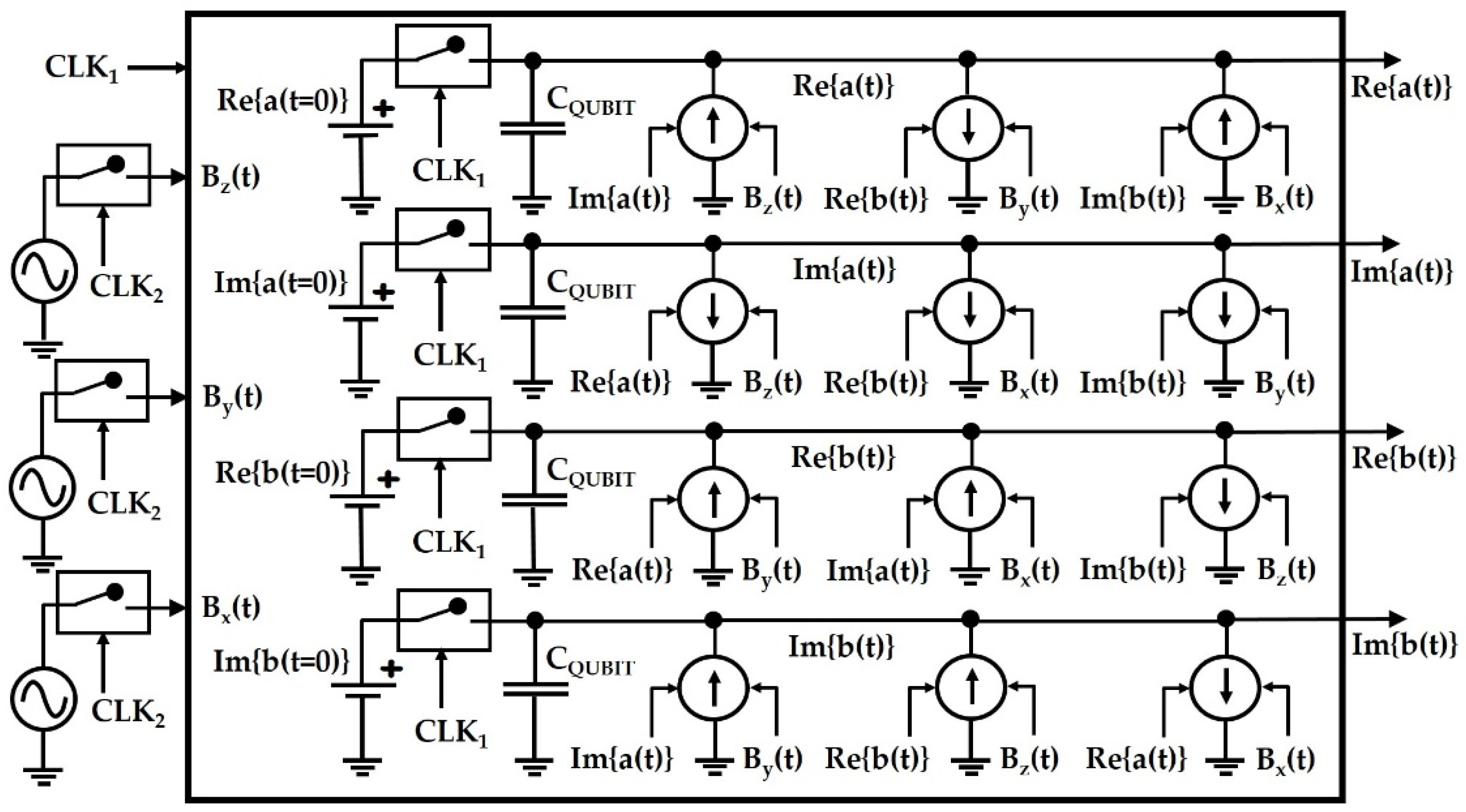
These four equations can be described through the equivalent electrical circuit depicted in Figure 1, in which the voltages are dimensionless and the currents are expressed in Tesla. Four capacitors, CQUBIT, all of an identical value equal to 2ħ/gμB = 11.37 Tps (h = 6.626 × 10⁻³⁴ Js, g = 2, and μB = 9.27 × 10⁻²⁴ J/T), are present in the circuit. The real and imaginary parts of a(t) and b(t) are the voltages across these CQUBIT capacitors (e.g., Re{a(t)} is the voltage across capacitor CQUBIT in the first differential equation) and the current flowing through these capacitors accounts for the left term of each differential equation. The twelve multiplying current sources implement the right terms in the differential equations.
The four DC generators in the model force the initial conditions Re{a(t = 0)}, Im{a(t = 0)}, Re{b(t = 0)}, and Im{b(t = 0)} under the control of clock CLK1. Another clock, CLK2, controls the application of the three magnetic field components Bx(t), By(t), and Bz(t), which are the inputs to the model (on the left) together with the CLK1; the model outputs are Re{a(t)}, Im{a(t)}, Re{b(t)}, and Im{b(t)} (on the right). The model thus exhibits four inputs and four outputs. At the start of the simulation, when the initial conditions are to be applied, the CLK1 closes the switches inside the model while the CLK2 keeps open the external ones. The moment the magnetic field is applied, CLK2 closes the external switches while CLK1 opens the internal ones.
To the best of the author’s knowledge, this is the first effort reported in the literature to model the behaviour of an electron spin qubit with such an approach. The qubit SPINE emulator proposed in [37,38] is indeed a physics-based compact model coding the qubit hamiltonian in Verilog-A. The equivalent circuit in Figure 1 is an innovative approach also with respect to the simulations of qubit gates based on C, Matlab or Python codes. Despite being few and not addressing the electron spin qubit, other qubit models are reported in the literature, in particular, to convert the behaviour of charge qubits into an equivalent circuit [43]. It is also worth remarking that in this paper, the authors identify a model at the core of which are voltage-controlled current sources. These sources are reported as time-varying, while in the model proposed in the present paper, the current sources generate currents proportional to the product of two voltages, one corresponding to a component of the magnetic field and the other to a component of the qubit state, as depicted in Figure 1. Equivalently, these sources may be described as time-varying voltage-controlled current sources in which the time-varying behaviour is forced by the magnetic field component while the qubit state component acts as the controlling input voltage. Interestingly, two different physical approaches, indipendently carried out on two different types of qubits, convergence on a set of voltage-controlled time-varying or equivalently multiplying current sources. In both the cases, the currents generated by these sources are integrated on a capacitor. In the present paper, the adopted mathematical physics approach allows us to trace back the capacitance of this capacitor to two fundamental constants: the Planck constant and the Bohr magneton. It is worth closing this section with a historical perspective. In the mid-fourties of the XX century, when computers were not yet available (in 1944, Alan Turing was designing vacuum-triodes-based Colossus to break the Enigma cipher), a physical analog approach was the only possible way to numerically solve the Maxwell [44] and the Schrödinger [45] differential equations. Kron used RLC bidimensional and tridimensional electrical circuits. Resorting to passive circuits was a necessity, as the transistor effect was yet to be discovered (which happened on the day before Christmas eve in 1947). In Kron’s approach, current sources are therefore not present. More recently, RLC circuits demonstrated their validity in quantum mechanics as an emulation tool of quantum gates [46]. In this approach, the voltage-controlled current sources are present but they are not time-varying or multiplying. Therefore, time-varying/multiplying current sources appear to be specific to the approach used in the present paper for the electron spin qubit and in [43] for the charge qubit.
3. Cadence© Implementation
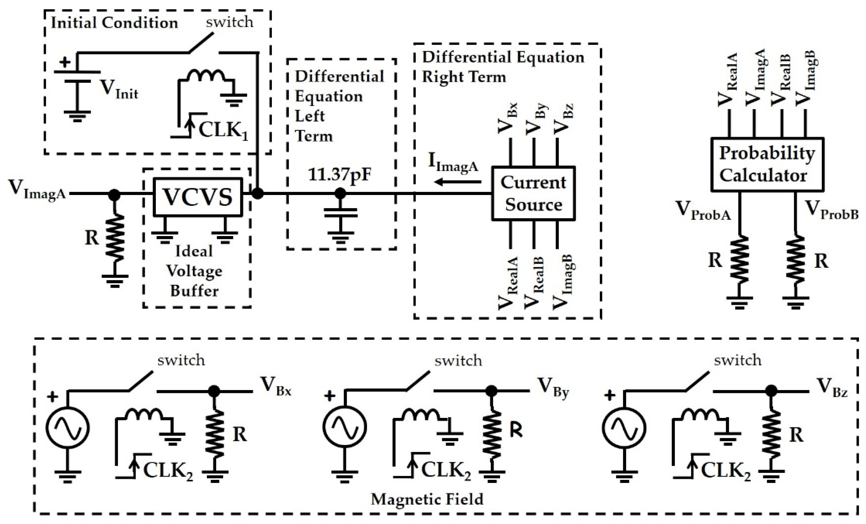
The proposed qubit compact model was implemented in Cadence©. The upper left corner of Figure 2 depicts the implementation of the sub-circuit concerning the imaginary part of a(t) in Figure 1. In this implementation, the voltage signal VImagA, corresponding to Im{a(t)} in Figure 1, is generated by integrating, on a capacitor with capacitance equal to 11.37 pF, the current IImagA generated by the current source, which was coded in Verilog-A. It is worth noting that in other circuit simulators (e.g., Quite Universal Circuit Simulator), these sources can be implemented through so-called Equation Defined Device/Sources [47]. As illustrated in Figure 2, the magnetic field components applied to the qubit are implemented as the voltage signals VBx, VBy, and VBz, which are the input of the current source block. The current source also receives as input the voltage signal VRealA, corresponding to Re{a(t)} in Figure 1, voltage signal VRealB, corresponding to Re{b(t)} in Figure 1, and voltage signal VImagB, corrsponding to Im{b(t)} in Figure 1. Each of these three voltage signals, VRealA, VRealB, and VImagB, are generated by a circuit identical to that depicted in Figure 2 for VImagA. All the current source blocks receive as input voltages VBx, VBy, and VBz, but in agreement with the model in Figure 1, the current source generating current IRealA receives voltage signals VImagA, VRealB, and VImagB, the current source generating current IImagB the voltage signals VImagA, VRealA, and VRealB, and the current source generating current IRealB the voltage signals VImagA, VRealA, and VImagB. As for the voltage signal VImagA, the voltage signals VRealA, VRealB, and VImagB are also made available at the output of an ideal voltage buffer implented by using a Voltage-Controlled Voltage Source (VCVS). This buffer isolates the capacitor upper plate, the most delicate node of the circuit, from the rest of the circuitry. The initial condition on this node is forced by applying a DC voltage source, as highlighted in the left upper corner. The switches are implemented with an open (close) resistance of 1 TΩ (1 nΩ).
The voltage sources generating signals VBx and VBy are the interface with the CMOS RFIC if voltage VBz accounts for the static component of the magnetic field. Physically speaking, the radiofrequency magnetic field is generated by radiofrequency current IRF circulating into a metallization line, operating as a microwave antenna placed close to the qubit (see for instance [48]). This current IRF is forced by a radiofrequency circuit that usually is constituted of an envelope generator, a vector modulator, and a radiofrequency local oscillator. During the design of an RFIC, the voltage sources for VBx and VBy are therefore replaced by the schematic of the RFIC cascaded with a block describing how the voltage signals generated by the RFIC circuit translate into the radiofrequency magnetic field.
4. Qubit Model Test
The model has been tested in the case of component Bz(t) being static and components Bx(t) and By(t) describing an electromagnetic field rotating in the plane normal to the static field. This circularly polarized magnetic field enables solving the differential equation system in the laboratory frame without invoking the rotating wave approximation. With Bz(t) = B0, Bx(t) = B1cosωt, and By(y) = B1sinωt from Equation (5), you obtain [49]:
where ω0 = gμBB0/2ℏ and ω1 = gμBB1/2ℏ. In order to induce prompt changes in the qubit state, frequency ω of the electromagnetic field should be set at the resonance frequency 2ω0, known as the Larmor frequency ωLarmor. As detailed in Appendix A, the solution of system (7) under the Larmor resonance condition obtains the following simple mathematical expressions for a(t) and b(t):
The probabilities of P0 and P1 of the qubit being in state |ψ0> and|ψ1>, respectively, are as follows:
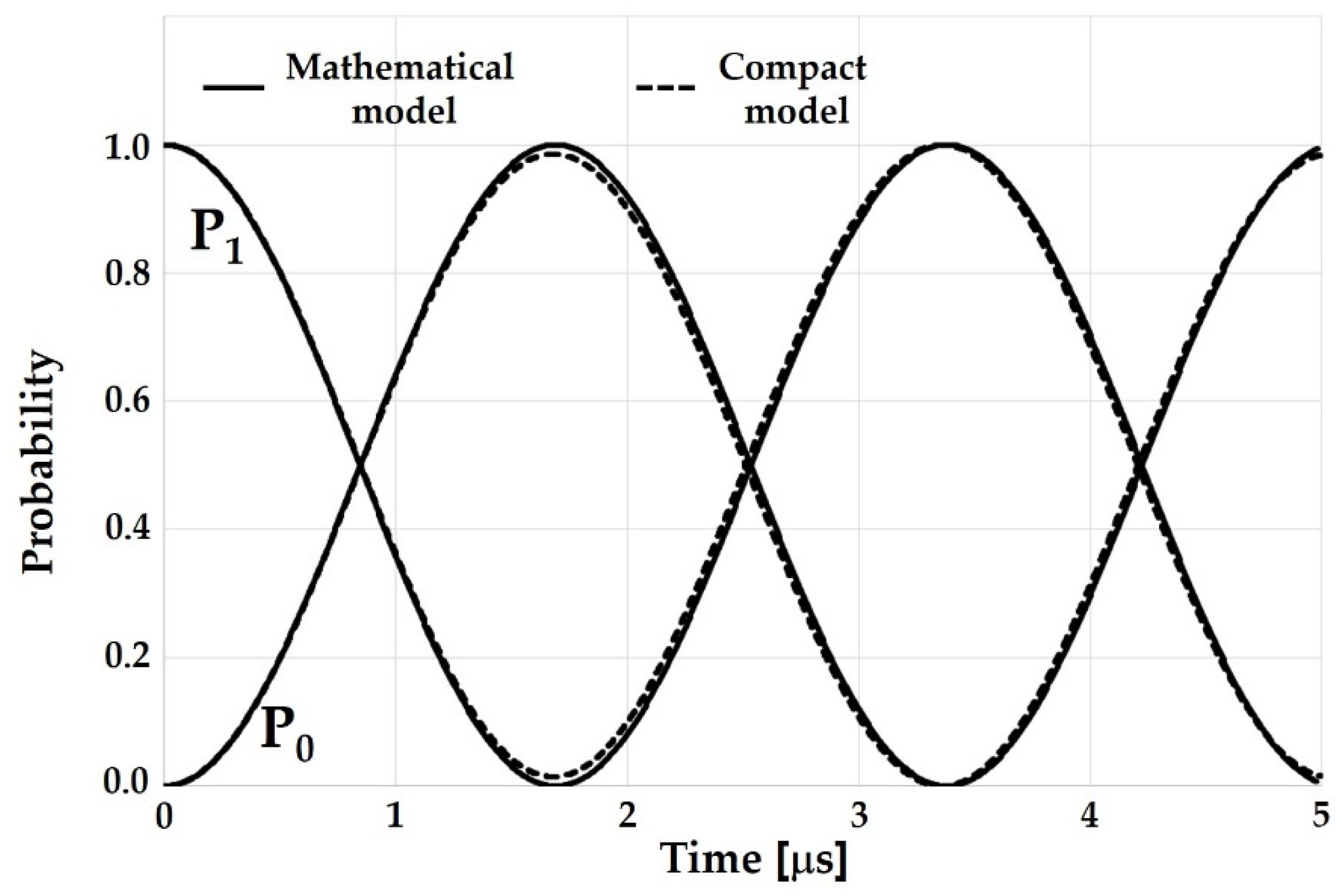
Each probability oscillates at frequency 2ω1, known as the Rabi frequency ωRabi, whose value depends on magnitude B1 of the rotating electromagnetic field and not on magnitude B0 of the static magnetic field. Figure 3 compares the oscillating P0 and P1 probabilities predicted by Equations (10) and (11) with the probabilities obtained from the Cadence© simulations of the proposed qubit compact model under resonance conditions for B0 = 1.4 mT and B1 = 10.6 μT. The simulations were carried out by using a trapezoidal integration method. The Euler integration method was avoided because it causes severe numerical damping. The convergence accuracy was set conservatively. In this way, the self-adaptive numerical algorithm adapts the actual time step for the best accuracy. It set the time step shorter (longer) when current or voltage variations in the circuit are large (small). The maximum time step was up-limited to 1ns. In addition, the amplitude of B1 was chosen in order to obtain typical values for ωRabi [50,51]. If the difference between B0 and B1 amplitudes is too large, possible numerical limitations in the simulation engine may make the terms multiplied by Bx and By negligible in the right terms of the differential equation system (6), leaving B0 as the only significant component. Under these conditions, the differential equation system is reduced to a couple of identical differential equations, each describing an oscillator at frequency ω0. Several numerical tests led to the conclusion that the amplitude difference between B0 and B1 should not be higher than two orders of magnitude in order to avoid the decoupling of the differential equations. Nevertheless, low values of B0, which are useful to avoid differential equations decoupling, may lead to ωLarmor lower than expected in a real case. In the co-simulation, this issue can be solved by means of an ideal frequency conversion of the signals generated by the RFIC circuit. It is worth nothing that, in the case of hot qubits, [51,52], the values of B0 found in the literature are in the order of 0.1 T, corresponding to ωLarmor in the range of a few GHz. Figure 3 shows that the qubit compact model correctly reproduces the sinusoidal behaviour predicted by the analytical solution. In particular, it is worth remarking that the model generates probability curves oscillating between 0 and 1, out of phase of π, and intersecting at 0.5, thus meeting the constraint P0 + P1 = 1. The best (worst) agreement between the compact model and the analytical solution of about 0.05% (1.4%) is achieved at 3.40 μs (1.70 μs). The Rabi frequency generated by the compact model is about 296.7 kHz, close to the 296.6 kHz value predicted by the mathematical expression of 2ω1.
In order to investigate further possible numerical issues, in addition to the previously discussed B0/B1 ratio, further simulation tests were carried out under off-resonance condition, by introducing a given amount of frequency offset Δω. The goal is to plot the qubit state probability, P0 or P1, versus Δω, when the qubit is excited with a microwave pulse of duration τp corresponding to one of the peak in the Rabi oscillation (e.g., for the probability P0, τp = 5.067 μs corresponds to the second peak in Figure 3).
The mathematics in the Appendix A shows that the probability P0(τp) obtained after having applied, to the electron spin qubit, a microwave pulse with a frequency offset Δω for a duration of τp = Ntπ, where N is an integer number and tπ is the pulse duration making the probability transits from 0 to 1, or from 1 to 0, under resonance conditions, exhibits the following mathematical expression:
which is known as the Rabi formula [53].
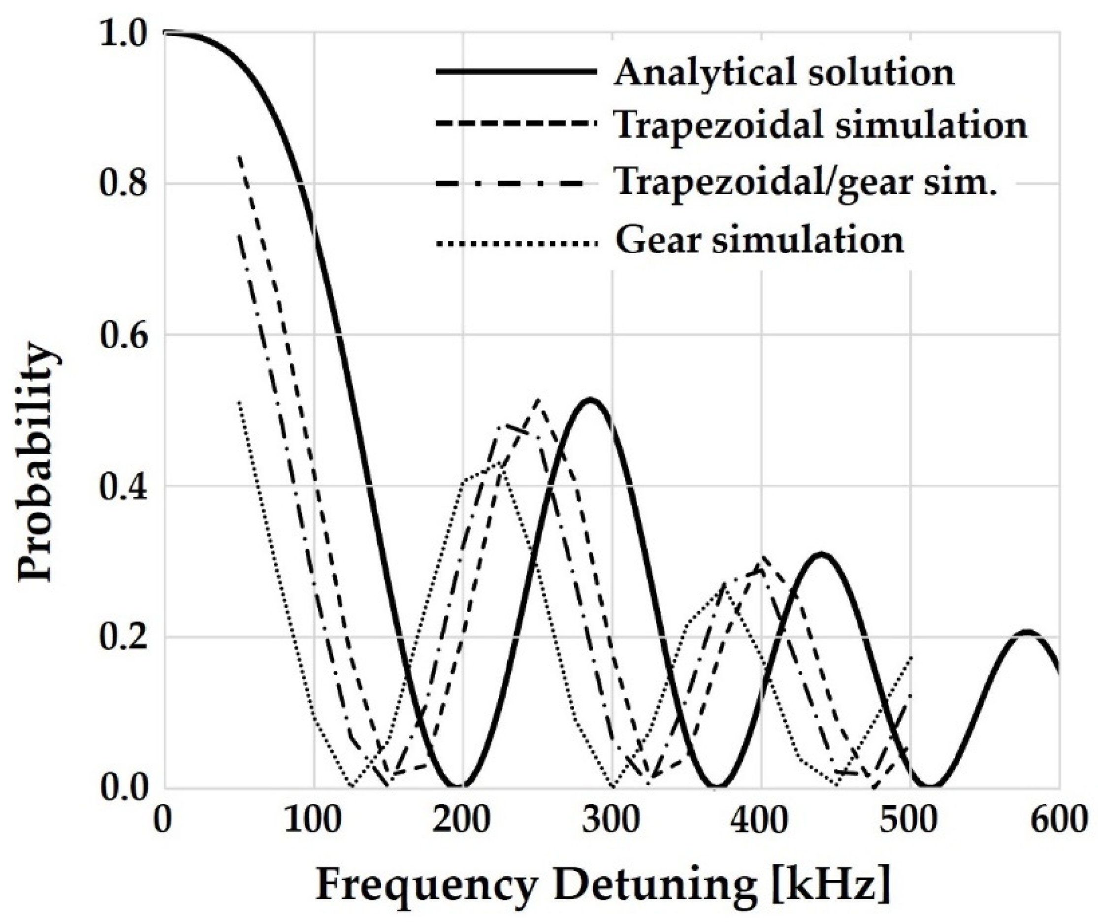
These curves are the cross sections on the discrete set of pulse durations πN/2ω1 of the chevron pattern, which is the surface generated by plotting P0 versus Δω and τp. Therefore, from this point on, these cross-section curves will be referred to as the chevron cross-sections. Figure 4 compares the chevron cross-sections predicted by Equation (12) with those generated by the qubit compact model for τp = 5.067 μs and for Δω up to 600 kHz. The figure shows that the simulated and analytically calculated cross-sections are frequency shifted.
In order to investigate the nature of this frequency shift, simulations were carried out by adopting different integration methods. Figure 4 shows that the degree of frequency shift depends on the adopted integration method, suggesting its numerical nature. Transient simulations are known indeed to be highly sensitive to the numerical method adopted to integrate nodal equations [54]. Figure 4 shows that the trapezoidal method leads to the lowest frequency shift, estimated as 35 kHz, while the gear (mixed trapezoidal gear) integration method leads to a frequency shift of about 68 kHz (50 kHz). This finding is in agreement with the fact that the trapezoidal integration method is usually the most efficient for a high accuracy [55]. In particular, the replacement of the continuous time derivative with a finite-difference approximation leads to a numerical error known as a local truncation error. This depends on the integration method and how it accumulates in the time depends on the circuit under simulation. In the case of an oscillator, it may cause phase drift. Since the chevron cross-sections come from oscillating probability waveforms computed through transient simulations where a microwave pulse is applied, under a given amount of frequency offset, for a fixed amount of time, a phase drift may turn out into a frequency shift in the chevron cross-sections.
Figure 5 shows that when the simulated chevron cross-sections are compensated forwith a 35-kHz frequency shift, the simulated trapezoidal chevron cross-section perfectly fits the analytical solution, which is not true for the other two cases. Indeed, the chevron cross-sections simulated with the gear and the gear-trapezoidal integration method not only still suffer from frequency detuning but also from being of lower local maxima than those predicted by the analytical solution. The disagreement is about 16.7% for the first peak and in the range of 6% for the second one. Since this disagreement is observed only when a gear component in the integration method is present, it appears to be reasonable to ascribe this disagreement in the local maxima to numerical damping, from which the gear integration method suffers even if it is as severe as in the case of the Euler integration method.
With the aim of testing the general validity of the 35 kHz frequency shift previously obtained for a maximum frequency offset of 600 kHz on the second Rabi peak, this frequency shift was applied to chevron cross-sections simulated for a larger frequency offset, up to about 1.5 MHz, and for different peaks of the Rabi oscillations. In all simulations, the adopted integration method was trapezoidal.
Figure 6, Figure 7 and Figure 8 depict the chevron cross-sections simulated for the first, second, and third peaks of the Rabi oscillations, corresponding to a τp of 1.689 μs, 5.067 μs, and 8.445 μs, respectively.
All the figures reveal a good agreement between the analytical solution and the compact model, proving the general validity of the 35 kHz frequency shift and supporting the hypothesis that the frequency shift stems from numerical issues.
5. Conclusions
The present paper proposes a CAD-oriented circuit-based compact model for the electron spin qubit. Its equivalent circuit approach is innovative with respect to the very few examples reported in the literature of electron spin qubit physics-based compact models coded in Verilog A code and with respect to the simulations of qubit gates based on C, Matlab or Python codes. At the core of the proposed model for the electron spin qubit are voltage-controlled current sources, as in the case of a recently published compact model of a charge qubit. Interestingly, two different mathematical formal approaches to the qubit modeling, applied to two different types of qubits, convergence on the same core. This suggests that voltage-controlled time-varying or multiplying sources may be at the core of a circuit compact model also in the case of a transmonic qubit. The proposed circuit-based compact model was implemented in the Cadence© CAD suite and tested in the case of a circularly polarized radiofrequency magnetic field. The compact model was able to correctly reproduce the qubit state probabilities, which are counter-phase oscillating between 0 and 1. The comparison with the analytical solution of the qubit Schrödinger equation shows a discrepancy between the simulated and the analytically calculated probabilities in the range of 0.5%–1.4%, low enough to reasonably allow microelectronics designers to address the impact on the qubit control of the addressed circuit solutions, of the chosen technology design kit and of the fabrication tolerances (corner cases) [56]. In this regard, it is worth noting that the required threshold for the fidelity for quantum error correction using surface codes is in the range of 1% [57].
The simulations revealed two main limitations in the use of the proposed qubit compact model, both related to numerical issues. First, the difference between the magnitudes of the static magnetic field and that of the rotating magnetic field should be kept lower than two orders of magnitude. This limitation is not very compelling because the Rabi oscillation, which is the typical physical observable of interest, depends on the amplitude of the rotating magnetic field and not on that of the static field, whose amplitude can be kept lower during the simulation. On the other hand, the static magnetic field amplitude fixes the Larmor frequency. In a case where the adopted low value of the static magnetic field led to a Larmor frequency lower than the frequency generated by the designed electronic circuit, an ideal frequency conversion could be envisaged at the interface between the circuit and the qubit compact model. The second limitation revealed was a frequency shift between the chevron cross-sections predicted by the analytical solution and those generated by the compact model. It was observed that the magnitude of this frequency shift depends on the chosen integration method. The lowest shift of 35 kHz was achieved with a trapezoidal integration method. Both of these numerical limitations are worth of further investigation by implementing the qubit compact model in several CAD tools, where integration methods and convergence algorithms may differ. As the proposed compact model is based on an equivalent circuit, one can expect indeed that it can be implemented in several CAD tools.
In summary, the present paper demonstrates a circuit-based compact model for an electron qubit with potentialities that are good enough to be considered a promising approach in the design of RFIC for quantum computing applications. Eventually, it will be worth making a few last considerations about the validation of the proposed qubit model in the design of an RFIC. Beyond the comparison with the analytical solution of the Schrödinger equation, reported in the present paper, a validation of the proposed qubit model in the design of a RFIC needs, as briefly described in the last paragraph of Section 3, a magnetic field interface between the model of the qubit and the schematic of the RFIC, so that it is possible to relate the signals generated by the RFIC with the observe qubit behaviour.
Funding
This research received no external funding.
Data Availability Statement
All the data are reported/cited in the paper.
Conflicts of Interest
The author declares no conflict of interest.
Appendix A
In the system in Equation (7), the substitution of the first differential equation into the second one, yields a second order differential equation for a(t):
whose general solution is known to be in the form:
the quantities ν1 and ν2 being:
Once the initial conditions a(t = 0)=a0 and b(t = 0) = b0 set, the two constants c1 and c2 are:
In particular, for the specific initial conditions a0 = 0 and b0 = 1, the expressions for a(t) and b(t) are:
It is straightforward to verify that the constraint |a(t)|2 + |b(t)|2 = 1 is met. The application of the Larmor resonance condition (ω = 2ω0) in the previous two expressions for a(t) and b(t) yields the Equations (8) and (9).
More generally, Equation (A5) gives the following mathematical expression for the propability P0(τp) of finding the qubit in the state |ψ0> after the application of a microwave pulse at a generic frequency ω for a given time duration τp:
As only the pulse durations corresponding to the peaks in the Rabi oscillation are of interest, the microwave pulse duration can be expressed as τp = Ntπ, where N is an integer number and tπ is the pulse duration making the probability transits from 0 to 1, or from 1 to 0, under resonance conditions. This pulse flips the qubit from one state to the other one. By expressing the time duration tπ as π/2ω1, Equation (A7) becomes:
by defining the frequency offset Δω = ω − 2ω0, Equation (12) can be obtained.
References
- Feynman, R.P. Simulating Physics with Computers. Int. J. Theor. Phys. 1982, 21, 467–488. [Google Scholar] [CrossRef]
- Shor, P.W. Algorithms for Quantum Computation: Discrete Logarithms and Factoring. In Proceedings of the 35th Annual Symposium on Foundation of Computer Science, Washington, DC, USA, 20–22 November 1994; pp. 124–134. [Google Scholar] [CrossRef]
- Vandersypen, L.M.-K.; Steffen, M.; Breyta, G.; Yannoni, C.S.; Sherwood, M.H.; Chuang, I.L. Experimental realization of Shor’s quantum factoring algorithm using nuclear magnetic resonance. Nature 2001, 414, 883–887. [Google Scholar] [CrossRef] [PubMed] [Green Version]
- Grover, L.K. A fast quantum mechanical algorithm for database search. In Proceedings of the 28th Annual ACM Symposium on the Theory of Computing, Philadelphia, PA, USA, 22–24 May 1996; pp. 1–8. [Google Scholar] [CrossRef] [Green Version]
- Olson, J.; Cao, J.Y.; Romero, J.; Johnson, P.; Dallaire-Demers, P.-L.; Sawaya, N.; Narang, P.; Kivlichan, I.; Wasielewski, M.; Aspur-Guzik, A. Quantum Computation and Information for Chemistry. NSF Workshop 2016, arXiv:1706.05413. [Google Scholar]
- Bourzak, K. Chemistry is quantum computing’s killer app. Chem. Eng. News 2017, 95, 27–31. [Google Scholar]
- Cao, Y.; Romero, J.; Aspuru-Guzik, A. Potential of quantum computing for drug discovery. IBM J. Res. Dev. 2018, 62, 6:1–6:20. [Google Scholar] [CrossRef]
- Gill, D.; Garcia, J.M.; Swarup, V.; Hintennach, A. Enter the Quantum Decade. In Proceedings of the Consumer Electronics Show (CES), Las Vegas, NV, USA, 8 January 2020. [Google Scholar]
- Solgun, F. Microwave Engineer’s Guide to the Design of Superconducting Qubit Circuits. In Proceedings of the IEEE MTT-S International Microwave Symposium, Boston, MA, USA, 2–7 June 2019; pp. 263–366. [Google Scholar] [CrossRef]
- Arute, F.; Arya, K.; Babbush, R.; Bacon, D.; Bardin, J.C.; Barends, R.; Biswas, R.; Boixo, S.; Brandao, F.G.S.L.; Buell, D.A.; et al. Quantum Supremacy using a programmable superconducting processor. Nature 2019, 574, 505–511. [Google Scholar] [CrossRef] [PubMed] [Green Version]
- Hsu, J. CES 2018: Intel’s 49-Qubit Chip Shoots for Quantum Supremacy. IEEE Spectrum, 8 January 2018. [Google Scholar]
- Vandersypen, L. Dot-to-Dot Design. IEEE Spectrum, 4 September 2007; Volume 44, 42–47. [Google Scholar] [CrossRef]
- Loss, D.; DiVincenzo, D.P. Quantum Computation with quantum dots. Phys. Rev. A 1998, 57, 120–126. [Google Scholar] [CrossRef] [Green Version]
- Zwanenburg, F.A.; Dzurak, A.S.; Morello, A.; Simmons, M.Y.; Hollenberg, L.C.L.; Klimeck, G.; Rogge, S.; Coppersmith, S.N.; Eriksson, M.A. Silicon quantum electronics. Rev. Mod. Phys. 2013, 85, 961–1019. [Google Scholar] [CrossRef]
- Veldhorst, M.; Eenink, H.G.J.; Yang, C.H.; Dzurak, A.S. Silicon CMOS architecture for a spin-based quantum computer. Nat. Commun. 2017, 8, 1–8. [Google Scholar] [CrossRef]
- Reilly, D.J. Engineering the quantum-classical interface of solid-states qubits. npj Nat. Quantum Inf. 2015, 1, 1–10. [Google Scholar] [CrossRef] [Green Version]
- Charbon, E.; Sebastiano, F.; Babaie, M.; Vladimirescu, A.; Shahmohammadi, M.; Staszewski, R.B.; Homulle, H.A.R.; Patra, B.; van Dijk, J.P.G.; Incadela, R.M. Cryo-CMOS Circuits and Systems for Scalable Quantum Computing. In Proceedings of the IEEE International Solid State Circuits, San Francisco, CA, USA, 5–9 February 2017; pp. 264–266. [Google Scholar] [CrossRef]
- Vandersypen, L. Quantum Computing—The Next Challenge in Circuit and System Design. In Proceedings of the IEEE Integrated Solid-State Circuit Conference (ISSCC), San Francisco, CA, USA, 5–9 February 2017; pp. 24–26. [Google Scholar] [CrossRef]
- Geck, L.; Kruth, A.; Bluhm, H.; van Waasen, S.; Heinen, S. Control Electronics For Semiconductor Spin Qubits. Quantum Sci. Technol. 2020, 5, 1. [Google Scholar] [CrossRef]
- Bluhm, H.; Schreiber, L.R. Semiconductor spin qubits—A scalable platform for quantum computing. In Proceedings of the IEEE International Symposium on Circuits and Systems (ISCAS), Sapporo, Japan, 26–29 May 2019. [Google Scholar] [CrossRef]
- Prati, E.; Rotta, D.; Sebastiano, F.; Charbon, E. From the quantum Moore’s law toward silicon based universal quantum computing. In Proceedings of the IEEE International Conference on Rebooting Computing, Washington, DC, USA, 8–9 November 2017. [Google Scholar] [CrossRef]
- Patra, B.; Incandela, R.M.; van Dijk, J.P.G.; Homulle, H.A.R.; Song, L.; Shahmohammadi, M.; Staszewski, R.B.; Vladimirescu, A.; Babaie, M.; Sebastiano, F.; et al. Cryo-CMOS Circuits and Systems for Quantum Computing Applications. IEEE J. Solid-State Circuits 2018, 53, 309–321. [Google Scholar] [CrossRef] [Green Version]
- Bardin, J.C.; Jeffrey, E.; Lucero, E.; Huang, T.; Naaman, O.; Barends, R.; White, T.; Giustina, M.; Sank, D.; Roushan, P.; et al. A 28nm Bulk-CMOS 4-to-8GHz <2mW Cryogenic Pulse Modulator for Scalable Quantum Computing. In Proceedings of the IEEE International Solid State Circuits Conference (ISSCC), San Francisco, CA, USA, 17–21 February 2019; pp. 456–458. [Google Scholar] [CrossRef] [Green Version]
- Nielinger, D.; Christ, V.; Degenhardt, C.; Geck, L.; Grewing, C.; Kruth, A.; Liebau, D.; Muralidharan, P.; Schubert, P.; Vliex, P.; et al. SQUBIC1: An integrated control chip for semiconductor qubits. In Proceedings of the International Workshop on Silicon Quantum Electronics, Hillsboro, OR, USA, 18–20 August 2017. [Google Scholar]
- Charbon, E. Cryo-CMOS: 60 Years of Technological Advances towards Emerging Quantum Technologies. In Proceedings of the IEEE 45th European Solid-State Circuit Conference, Krakow, Poland, 23–26 September 2019. [Google Scholar]
- Bardin, J. CMOS Integrated Circuits for Control of Transmon Qubits. In Proceedings of the Tutorial at IEEE 45th European Solid-State Circuit Conference, Krakow, Poland, 23–26 September 2019. [Google Scholar]
- Voiginescu, S. Towards monolithic quantum computing processors in production FD-SOI CMOS technology. In Proceedings of the Tutorial at IEEE 45th European Solid-State Circuit Conference, Krakow, Poland, 23–26 September 2019. [Google Scholar]
- Sebastiano, F. Cryogenic CMOS interfaces for large-scale quantum computers: From system and device models to circuits. In Proceedings of the Tutorial at IEEE 45th European Solid-State Circuit Conference, Krakow, Poland, 23–26 September 2019. [Google Scholar]
- Mehrpoo, M.; Patra, B.; Gong, J.; Hart, P.A.; van Dijk, J.P.G.; Homulle, H.; Kiene, G.; Vladimirescu, A.; Sebastiano, F.; Charbon, E. Benefits and Challenges of Designing Cryogenic CMOS RF Circuits for Quantum Computers. In Proceedings of the IEEE International Symposium on Circuits and Systems (ISCAS), Sapporo, Japan, 26–29 May 2019. [Google Scholar] [CrossRef]
- Meunier, T. Towards scalable silicon quantum computing. In Proceedings of the Tutorial at IEEE 45th European Solid-State Circuit Conference, Krakow, Poland, 23–26 September 2019. [Google Scholar]
- Baugh, J. Network architecture for a surface code quantum computer in silicon. In Proceedings of the IEEE 45th European Solid-State Circuit Conference, Krakow, Poland, 23–26 September 2019. [Google Scholar]
- Degenhardt, C.; Artanov, A.; Geck, L.; Grewing, C.; Kruth, A.; Nielinger, D.; Vliex, P.; Zambanini, A.; van Waasen, S. Systems Engineering of Cryogenic CMOS Electronics for Scalable Quantum Computers. In Proceedings of the IEEE International Symposium on Circuits and Systems (ISCAS), Sapporo, Japan, 26–29 May 2019. [Google Scholar] [CrossRef]
- Lehmann, T. Cryogenic Support Circuits and Systems for Silicon Quantum Computers. In Proceedings of the IEEE International Symposium on Circuits and Systems (ISCAS), Sapporo, Japan, 26–29 May 2019. [Google Scholar] [CrossRef]
- Jazaeri, F.; Beckers, A.; Tjalli, A.; Sallese, J.-M. A Review on Quantum Computing: From Qubits to Front-end Electronics and Cryogenic MOSFET Physics. In Proceedings of the IEEE International Conference on Mixed Design of Integrated Circuits and Systems, Rzeszow, Poland, 27–29 June 2019; pp. 15–25. [Google Scholar] [CrossRef]
- Severino, R.R.; Spasaro, M.; Zito, D. Silicon Spin Qubit Control and Readout Circuits in 22nm FDSOI CMOS. In Proceedings of the IEEE International Symposium on Circuits and Systems (ISCAS), Seville, Spain, 12–14 October 2020. [Google Scholar] [CrossRef]
- Charbon, E.; Babaie, M.; Vladimirescu, A.; Sebastiano, F. Cryogenic CMOS Circuits and Systems. IEEE Microw. Mag. 2021, 22, 60–78. [Google Scholar] [CrossRef]
- Van Dijk, J.; Vladimirescu, A.; Babaie, M.; Charbon, E.; Sebastiano, F. A Co-design Methodology for Scalable Quantum Processors and their Classical Electronic Interface. In Proceedings of the Design, Automation & Test in Europe Conference, Dresden, Germany, 19–23 March 2018; pp. 573–576. [Google Scholar] [CrossRef]
- Van Dijk, J.; Vladimirescu, A.; Babaie, M.; Charbon, E.; Sebastiano, F. SPINE (SPIN Emulator)—A Quantum-Electronics Interface Simulator. In Proceedings of the IEEE International Workshop on Advances in Sensors and Interfaces (IWASI), Lecce, Italy, 13–14 June 2019; pp. 23–28. [Google Scholar] [CrossRef]
- Feynman, R.P.; Leighten, R.B.; Sands, M. The Feynman Lectures on Physics; Addison-Wesley Publishing Company Inc.: Oxnard, CA, USA, 1964; Volume 3, ISBN-10 8131792137. [Google Scholar]
- Pauli, A.M. The Principles of Quantum Mechanics; Oxford University Press: New York, NY, USA, 1947; ISBN 9783540098423. [Google Scholar]
- Tahan, C.; Friesen, M.; Joyint, R. Decoherence of electron spin qubits in Si-based quantum computers. Phys. Rev. B 2002, 66, 035314. [Google Scholar] [CrossRef] [Green Version]
- Tarasov, L.V. Basic Concepts of Quantum Mechanics; MIR Publishers: Moscow, Russia, 1980; ISBN 9785396002920. [Google Scholar]
- Blokhina, E.; Sokolov, A.; Giounanlis, P.; Wu, X.; Bashir, I.; Leipold, D.; Bogdan Staszewski, R.; Brambilla, A.; Bizzarri, F. Towards the Co-Simulation of Charge Qubits: A Methodology Grounding on an Equivalent Circuit Representation. IEEE Open J. Circuits Syst. 2021, 2, 548–563. [Google Scholar] [CrossRef]
- Kron, G. Equivalent Circuit of the Field Equations of Maxwell. Proc. IRE 1944, 5, 289–299. [Google Scholar] [CrossRef]
- Kron, G. Electric Circuit Models of the Schrödinger Equation. Phys. Rev. 1945, 67, 39–43. [Google Scholar] [CrossRef]
- Moxley, I.M. Quantum Port-Hamiltonian Network Theory. Royal Society Publishing 2000. Available online: http://hal.archives-ouvertes.fr/hal-02554914/document (accessed on 10 December 2021).
- Brinson, M.; Kusnetsov, V. Device and Component Modelling with Algebraic Equations. Available online: qucs-help.readthedocs.io/en/spice4qucs/DModel.html (accessed on 10 December 2021).
- Hwang, J.C.C.; Yang, C.H.; Veldhorst, M.; Hendrickx, N.; Fogarty, M.A.; Huang, W.; Hudson, F.E.; Morello, A.; Dzurak, A.S. Impact of g-factors and valleys on spin qubits in a silicon double quantum dot. Phys. Rev. B 2017, 96, 1–7. [Google Scholar] [CrossRef] [Green Version]
- Cohen-Tannoudji, C.; Dui, B.; Laloe, F. Quantum Mechanics; Wiley: New York, NY, USA, 1977; ISBN-10 047116433X. [Google Scholar]
- Veldhorst, M.; Hwang, J.C.C.; Yang, C.H.; Leenstra, A.W.; de Ronde, B.; Dehollain, J.P.; Muhonen, J.T.; Hudson, F.E.; Itoh, K.M.; Morello, A.; et al. An addressable quantum dot qubit with fault-tolerant control-fidelity. Nat. Nanotechnol. 2014, 9, 981–985. [Google Scholar] [CrossRef] [Green Version]
- Petit, L.; Eenink, H.G.J.; Russ, M.; Lawrie, W.I.L.; Hendrickx, N.W.; Philips, S.G.J.; Clarke, J.S.; Vandersypen, L.M.K.; Veldhorst, M. Universal quantum logic in hot silicon Qubits. Nature 2020, 580, 355–359. [Google Scholar] [CrossRef] [Green Version]
- Yang, C.H.; Leon, R.C.C.; Hwang, J.C.C.; Saraiva, A.; Tanttu, T.; Huang, W.; Camirand Lemyre, J.; Chan, K.W.; Tan, K.Y.; Hudson, F.E.; et al. Operation of silicon quantum processor unit cell above one Kelvin. Nature 2020, 580, 350–354. [Google Scholar] [CrossRef] [PubMed] [Green Version]
- Rabi, I.I. Space Quantization in a Gyrating Magnetic Field. Phys. Rev. 1937, 51, 652–654. [Google Scholar] [CrossRef]
- Introduction to Analogue IC Design, Simulation, Layout and Verification; Lecture Book Microelectronics Support Centre, STFC Rutherford Appleton Laboratory: Oxford, UK, 2019.
- Spectre Circuit Simulator Reference, Product Version 19.1; Cadence Design System Inc.: San Jose, CA, USA, 2020.
- Van Dijk, J.P.-G.; Kawakami, E.; Schouten, R.N.; Veldhorts, M.; Vandersypen, L.M.K.; Babaie, M.; Charbon, E.; Sebastiano, F. Impact of Classical Control Electronics on Qubit Fidelity. Phys. Rev. Appl. 2019, 12, 044054. [Google Scholar] [CrossRef] [Green Version]
- Fowler, A.; Marlantoni, M.; Martinis, J.M.; Cleland, A.N. Surface codes: Towards practical large-scale quantum computation. Phys. Rev. A 2012, 86, 1–48. [Google Scholar] [CrossRef] [Green Version]
Figure 1.
Compact model of the electron spin qubit.

Figure 2.
Implementation of the compact model in Figure 1.
Figure 2.
Implementation of the compact model in Figure 1.

Figure 3.
Compact model simulated vs analytically calculated Rabi oscillations.

Figure 4.
Chevron cross-sections for P0 for the second peak of the Rabi oscillation (τp = 5.067 μs).
Figure 4.
Chevron cross-sections for P0 for the second peak of the Rabi oscillation (τp = 5.067 μs).

Figure 5.
35 kHz frequency compensated simulated chevron cross-sections vs. analytical chevron cross-section for P0 for the second peak of the Rabi oscillation (τp = 5.067 μs) in the case of different integration method.
Figure 5.
35 kHz frequency compensated simulated chevron cross-sections vs. analytical chevron cross-section for P0 for the second peak of the Rabi oscillation (τp = 5.067 μs) in the case of different integration method.

Figure 6.
A 35-kHz frequency compensated simulated chevron cross-section vs. analytical chevron cross-section for P0 for the first peak of the Rabi oscillation (τp = 1.689 μs) in the case of trapezoidal integration method.
Figure 6.
A 35-kHz frequency compensated simulated chevron cross-section vs. analytical chevron cross-section for P0 for the first peak of the Rabi oscillation (τp = 1.689 μs) in the case of trapezoidal integration method.

Figure 7.
A 35 kHz frequency compensated simulated chevron cross section vs. analytical chevron cross-section for P0 for the second peak of the Rabi oscillation (τp = 5.067 μs) in the case of trapezoidal integration method.
Figure 7.
A 35 kHz frequency compensated simulated chevron cross section vs. analytical chevron cross-section for P0 for the second peak of the Rabi oscillation (τp = 5.067 μs) in the case of trapezoidal integration method.

Figure 8.
A 35 kHz frequency compensated simulated chevron cross-section vs. analytical chevron cross-section for P0 for the third peak of the Rabi oscillation (τp = 8.445 μs) in the case of trapezoidal integration method.
Figure 8.
A 35 kHz frequency compensated simulated chevron cross-section vs. analytical chevron cross-section for P0 for the third peak of the Rabi oscillation (τp = 8.445 μs) in the case of trapezoidal integration method.

Publisher’s Note: MDPI stays neutral with regard to jurisdictional claims in published maps and institutional affiliations. |
© 2022 by the author. Licensee MDPI, Basel, Switzerland. This article is an open access article distributed under the terms and conditions of the Creative Commons Attribution (CC BY) license (https://creativecommons.org/licenses/by/4.0/).
Share and Cite
MDPI and ACS Style
Borgarino, M. Circuit-Based Compact Model of Electron Spin Qubit. Electronics 2022, 11, 526. https://0-doi-org.brum.beds.ac.uk/10.3390/electronics11040526
AMA Style
Borgarino M. Circuit-Based Compact Model of Electron Spin Qubit. Electronics. 2022; 11(4):526. https://0-doi-org.brum.beds.ac.uk/10.3390/electronics11040526
Chicago/Turabian StyleBorgarino, Mattia. 2022. "Circuit-Based Compact Model of Electron Spin Qubit" Electronics 11, no. 4: 526. https://0-doi-org.brum.beds.ac.uk/10.3390/electronics11040526
Note that from the first issue of 2016, this journal uses article numbers instead of page numbers. See further details here.