
Observational Constraints and Some Toy Models in f(Q) Gravity with Bulk Viscous Fluid


1
Department of Mathematics, Birla Institute of Technology and Science-Pilani, Hyderabad Campus, Hyderabad 500078, India
2
International College of Liberal Arts, Yamanashi Gakuin University, Yamanashi 400-0805, Japan
*
Author to whom correspondence should be addressed.
Universe 2022, 8(4), 240; https://0-doi-org.brum.beds.ac.uk/10.3390/universe8040240
Submission received: 9 March 2022
/
Revised: 6 April 2022
/
Accepted: 11 April 2022
/
Published: 13 April 2022
(This article belongs to the Special Issue Cosmology in the High-Precision Era: Observations, Theory, and Their Symbiosis)
Abstract
:The standard formulation of general relativity fails to describe some recent interests in the universe. It impels us to go beyond the standard formulation of gravity. The gravity theory is an interesting modified theory of gravity, where the gravitational interaction is driven by the nonmetricity Q. This study aims to examine the cosmological models with the presence of bulk viscosity effect in the cosmological fluid within the framework of gravity. We construct three bulk viscous fluid models, i.e., (i) for the first model, we assuming the Lagrangian as linear dependence on Q, (ii) for the second model the Lagrangian as a polynomial functional form, and (iii) the Lagrangian as a logarithmic dependence on Q. Furthermore, we use 57 points of Hubble data and 1048 Pantheon dataset to constrain the model parameters. Then, we discuss all the energy conditions for each model, which helps us to test the self-consistency of our models. Finally, we present the profiles of the equation of state parameters to test the models’ present status.
1. Introduction
The current accelerated expansion scenario of the universe is still far from being understood [1,2,3,4]. This problem motivated the research community to go beyond Einstein’s general theory of relativity (GR) to describe the candidates responsible for the present scenarios, namely dark energy and dark matter. In GR, the addition of cosmological constant in field equations helps us to understand the unknown form of energy, but it faces some issues such as the coincidence problem and the fine-tuning problem; its effects are only observed at cosmological scales (the current accelerated expansion phase) instead of Planck scales [5]. Therefore, in the last few decades, several alternative proposals have been presented in the literature to overcome the current issues of the universe and explore new insights into the universe.
Recently, a novel proposal has been proposed by Jimenez et al. [6], namely symmetric teleparallel gravity or gravity, where the fundamental of gravitational interaction is described by the nonmetricity Q. Studies on gravity are being developed in large numbers and there are observational constraints against standard GR formalism.
An interesting work on symmetric teleparallel gravity was done by Lazkoz et al. [7], where a set of functions were constrained. To do that, they reformulated the Lagrangian as a function of redshift z and discussed the observational constraints using data from gamma-ray bursts, early-type galaxies, cosmic microwave background, type Ia supernovae, baryon acoustic oscillations, and quasars. A relevant study on gravity was done by Mandal et al. [8] to understand its behavior using energy conditions, where energy conditions for gravity were derived and the self-stability of two models was tested. Also, they used the parametrization technique and cosmographic idea to constrain three cosmographic sets of functions using the largest Pantheon supernovae data through statistical analysis in gravity [9]. Indeed, some interesting studies were done using this modified theory (see details in [10,11,12,13,14]).
In the literature, most of the cosmological models are considered perfectly fluid when the matter content of the universe and its evolution is discussed. t is equally important to investigate more physically reliable models such as the dissipative phenomena, in the form of bulk viscosity, might affect the evolution history of the universe, which has been discussed regularly. However, the presence of bulk viscosity in a homogeneous and isotropic universe is capable of modifying the background dynamics. The viscous cosmological scenarios come into the picture after the introduction of relativistic thermodynamics. The standard expression for relativistic viscosity was obtained by Eckart in 1940 [15]. Later, its cosmological applications were investigated by Weinberg [16] and Treciokas and Ellis [17]. Then, the bulk viscosity was used to explore the universe’s early evolution, whether in the case of the neutrino decoupling process or the inflation epoch. In the 1970s, various cosmological applications of bulk viscous imperfect fluid have been discussed [18,19,20,21]. An imperfect fluid with bulk viscosity can also describe the acceleration of the universe without the presence of a scalar field or cosmological constant [22,23,24,25]. Further, an inflation process that can be explained with viscous pressure was proposed in 1980s [26,27,28,29]. Also, it is well-known that the Israel-Stewart approach is used in many studies to explore causality in relation to the bulk viscous matter [for instance one can see [30,31,32]. Moreover, the bulk viscosity of the cosmic fluid produces effective pressure when it expands faster than the system to restore its thermal stability [33]. The effective pressure can be treated as bulk viscosity. In an accelerated expanding universe it may be natural to assume the possibility that the expansion process is actually a collection of states out of thermal equilibrium in a small fraction of time due to the existence of a bulk viscosity [34]. In addition, the bulk viscosity produces effective negative pressure, which could be considered a suitable candidate for the current accelerated expansion of the universe [25,35,36,37,38]. It is worth mentioning here that bulk viscosity can describe both dark matter and dark energy simultaneously [25,39,40]. The possibility of violating the dominant energy condition (DEC) is a well-known result of the FRW cosmological solutions, which correspond to a universe filled with perfect fluid and bulk viscous stresses. The debate over bulk viscosity is reasonable and practical when it comes to the late time expansion of the universe as we do not know the nature of dark energy and dark matter. Such a possibility only has been investigated in the context of the primordial universe and non-singular model searches. Therefore, we aim to study the current accelerated expansion of the universe by introducing the bulk viscosity of the cosmic fluid under the framework of the modified theory of gravity.
In this study, we have added the bulk viscosity effect in the cosmological fluid to explore the universe’s present scenario. It is well known that the late-time cosmic acceleration is driven by negative pressure, and the bulk viscous fluid also negatively affects the pressure. This might help us understand the universe’s current expansion through gravity. The advantage of working on this theory over the teleparallel theory is that the connections admit freely specifiable functions, and these free functions are promoted to true connection degrees of freedom, whereas teleparallel connections are completely fixed. They not only enter the metric field equations but also possess their equations of motion, and they genuinely influence the gravitational field. Therefore, it is adequate to say that cosmology is more valuable than cosmology at the background level because of these additional degrees of freedom. The above case is true for flat and non-flat spatial cases. A possible explanation is that while both connections in and gravity respect homogeneity and isotropy and are flat, the connection also has to satisfy the conditions . These are 40 independent equations, as opposed to the 24 independent equations the connection has to satisfy because of the conditions . Hence, the connection is generally more restricted than the connection. In literature, many studies have been done on the bulk viscous fluid to deal with the present issues of the universe. For instance, Arora et al. [41] studied bulk viscosity models in gravity, where stability analysis of the cosmological models have been examined by focusing on the current phase as well as tested against the observational data from Union 2.1 type Ia supernovae and Hubble data. The cosmic expansion is studied with matter creation and bulk viscosity in [42]. Here, we are focusing on investigating the stability analysis of the bulk viscous fluid models in modified gravity in correspondence with the universe’s present scenario.
This article is organized as follows: in Section 2, we briefly discuss the gravity framework and derive the field equations for the bulk viscous fluid. Energy conditions are the greatest tool to test the self-stability of the cosmological models. We discuss the energy conditions for gravity in Section 3. In Section 4, we use Markov Chain Monte Carlo (MCMC) analysis to estimate the coefficients in the expression of . There the 57 Hubble data points and 1048 Pantheon supernovae dataset are used for simulation. The energy conditions of three viscous fluid models are examined in Section 5. Also, the equations of state parameters are discussed for each model in Section 5. Finally, we discuss the final outcomes and future perspectives in Section 6.
2. Geometrical Overview
Here, we have considered that the action for symmetric teleparallel gravity is given by [6]
where represents the function form of Q, g is the determinant of the metric , and is the matter Lagrangian density.
The non-metricity tensor and its traces can be written as
Also, the non-metricity tensor helps us to write the superpotential as
where the trace of non-metricity tensor [6] has the form
Again, by definition, the energy-momentum tensor for the fluid description of the spacetime cab be written as
Now, one can write the motion equations by varying the action (1) with respect to metric tensor , which can be written as
where . Also, varying (1) with respect to the connection, one obtains
The FLRW line element is given by
where is the scale factor of the universe. For this line element the trace of non-metricity tensor takes the following form:
We take the energy-momentum tensor of the cosmological fluid which is given by
where and represents the pressure with viscous fluid and represents the energy density. The physical unit of cosmological parameters is considered in the Planck scale.
Using (9) and (10) in (7) one can find the field equation as follows
where dot represents derivative with respect to t. The energy conservation equation for the viscous fluid can be written as
The equation of state (EoS) parameter can be written as
Now, one can use the above set up to explore the cosmological evolution of the universe, applying various approaches.
Here, and are the effective pressure and energy density of the fluid content, respectively. The previous equations are going to be components of a modified energy-momentum tensor , embedding the dependence on the trace of the nonmetricity tensor.
3. Energy Conditions
The energy conditions (ECs) are the essential tools to understanding the geodesics of the Universe. Such conditions can be derived from the well-known Raychaudhury equations, the forms of which are [43,44,45]
where is the expansion factor, is the null vector, and and are, respectively, the shear and the rotation associated with the vector field . In the Weyl geometry with the presence of non-metricity, the Raychaudhury equations takes different forms [see details calculations for the Raychaudhury equations with the non-metricity [46]. For attractive gravity, Equations (21) and (22) satisfy the following conditions
Therefore, if we are working with a perfect fluid matter distribution, the energy conditions for gravity are given by [8],
- Strong energy conditions (SEC) if ;
- Weak energy conditions (WEC) if ;
- Null energy condition (NEC) if ;
- Dominant energy conditions (DEC) if .
Taking Equations (19) and (20) into WEC, NEC, and DEC constraints, we are able to prove that
- Weak energy conditions (WEC) if ;
- Null energy condition (NEC) if ;
- Dominant energy conditions (DEC) if .
corroborating with the work from Capozziello et al. [47]. In the case of the SEC condition, we yield to the constraint
Now, using above energy conditions, we can test the viability of our cosmological models. Further, it will helps us to understand our universe in a more realistic way.
4. Data Interpretation
In this section, we adopted the parametrization technique, which will be used to reconstruct the cosmological models. Some interesting studies have used the parametrization technique to explore the cosmological models [48,49]. The main advantage of adopting this technique is that we can study the cosmological models with observational data. As we know, the relation between the scale factor and the redshift z is given by , where is the late time scale factor. From the above relation we can find . The non-metricity Q in term of redshift z can be written as , where , and the late time Hubble parameter km s Mpc [50].
The interesting work of Sahni et al. [51,52] motivates us to take the functional form of as follows:
where , and are constants. These constants can be measured by using the observational data. Also, we can find an additional constraint on the parameters for as .
4.1. Hubble Dataset
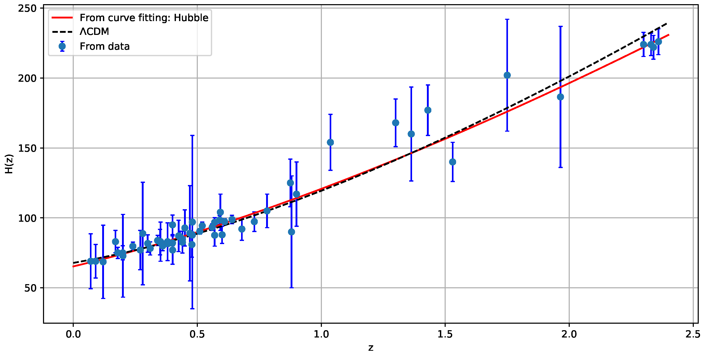
Recently, a list of 57 data points of the Hubble parameter in the redshift range were compiled by Sharov and Vasiliev [53]. This H(z) dataset was measured from the line-of-sight BAO data [54,55,56,57,58] and the differential ages of galaxies [59,60,61,62]. The complete list of datasets is presented in [53]. To estimate the model parameters, we used the Chi-square test by MCMC simulation. The Chi-square function is given by
where represents the observed Hubble parameter values, represents the Hubble parameter with the model parameters, and is the standard deviation.
4.2. Pantheon Dataset
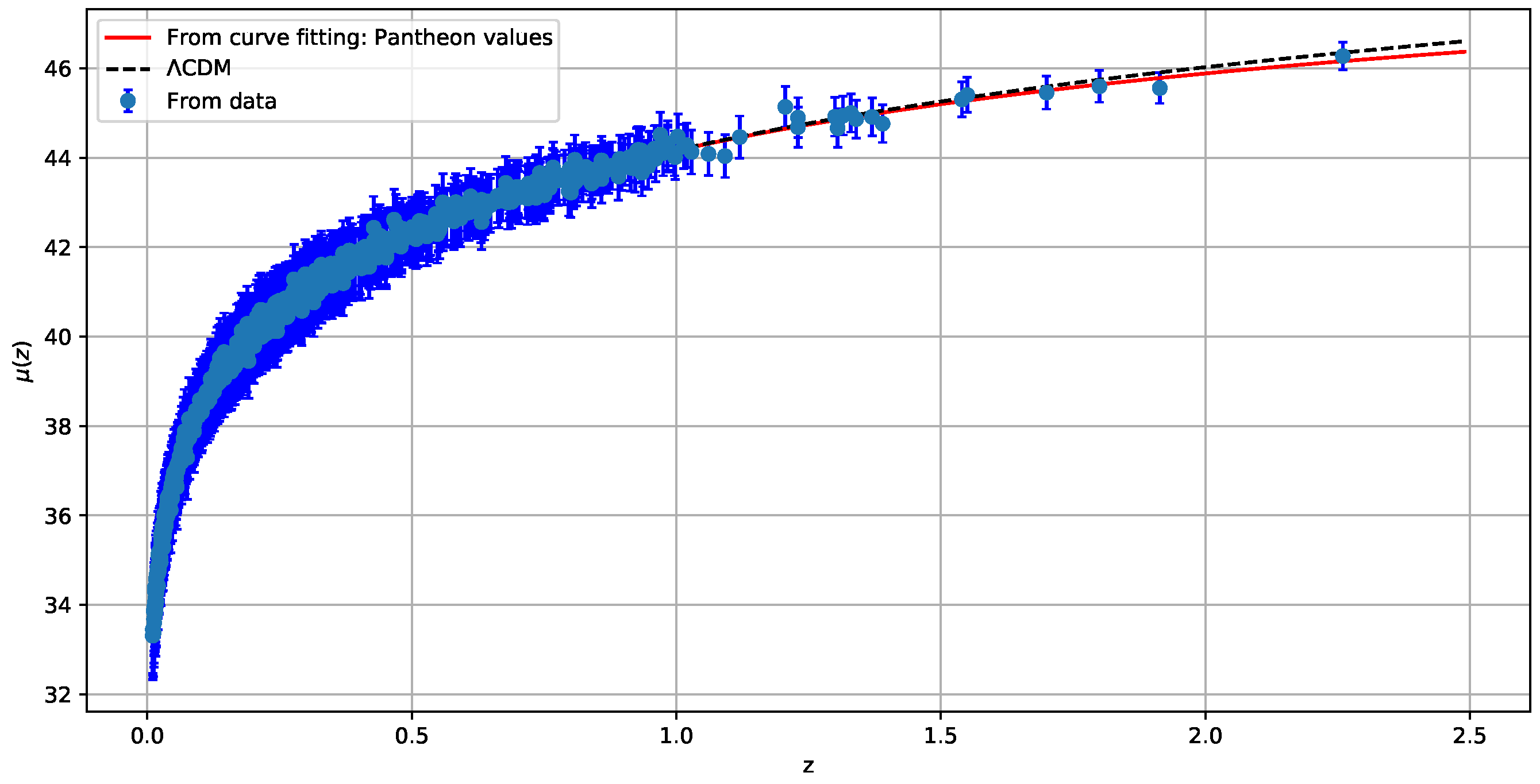
Here, we use the latest Pantheon supernovae type Ia sample, which contains 1048 SNe Ia data points from SNLS, SDSS, Pan-STARRS1, HST surveys, and low-redshift in the redshift-range to constraint the above parameters [63]. The function from the Pantheon sample of 1048 SNe Ia [63] is given by
where represents the free parameters of the presumed model and is the covariance metric [63], and represents the distance moduli is given by:
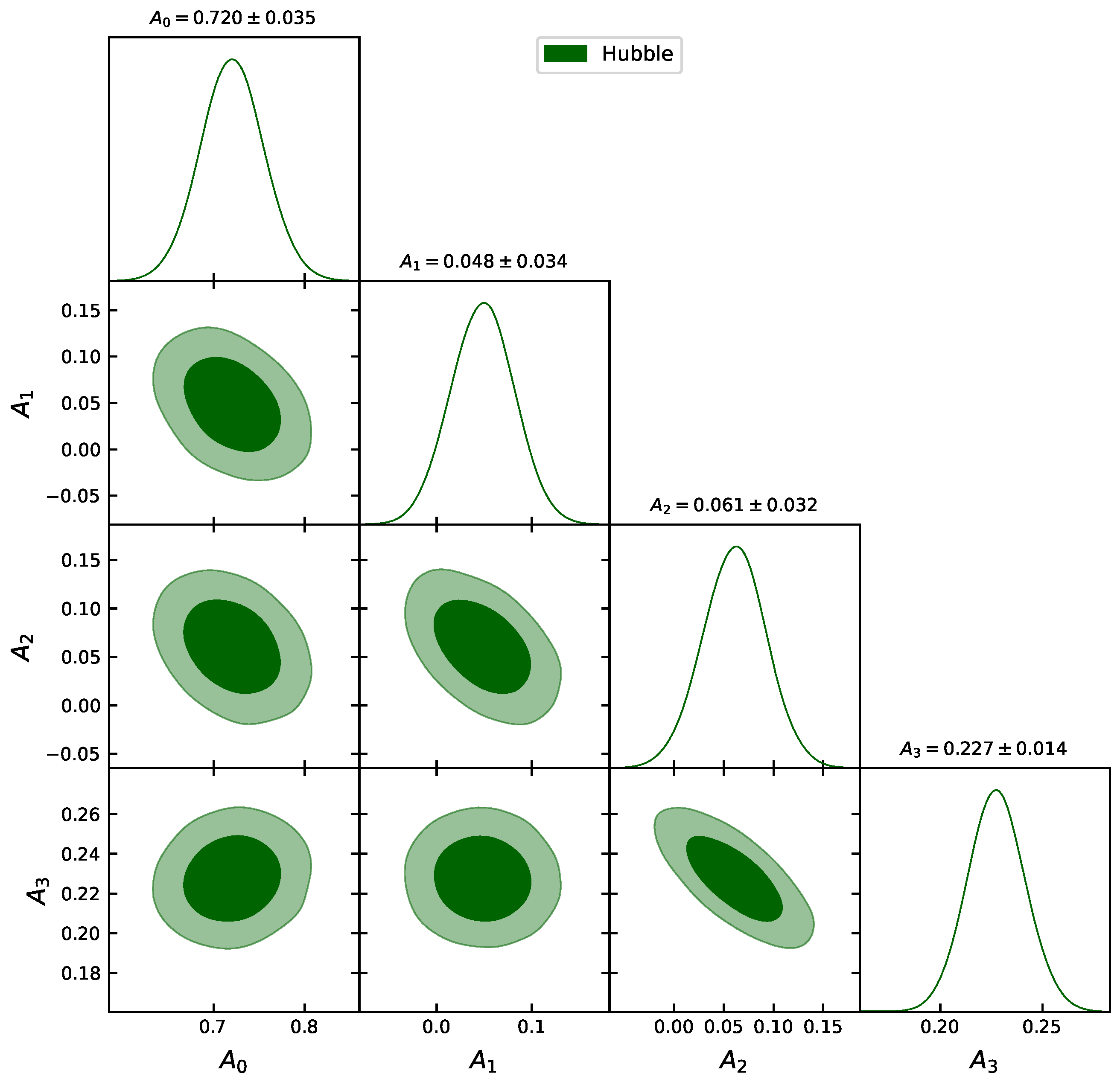
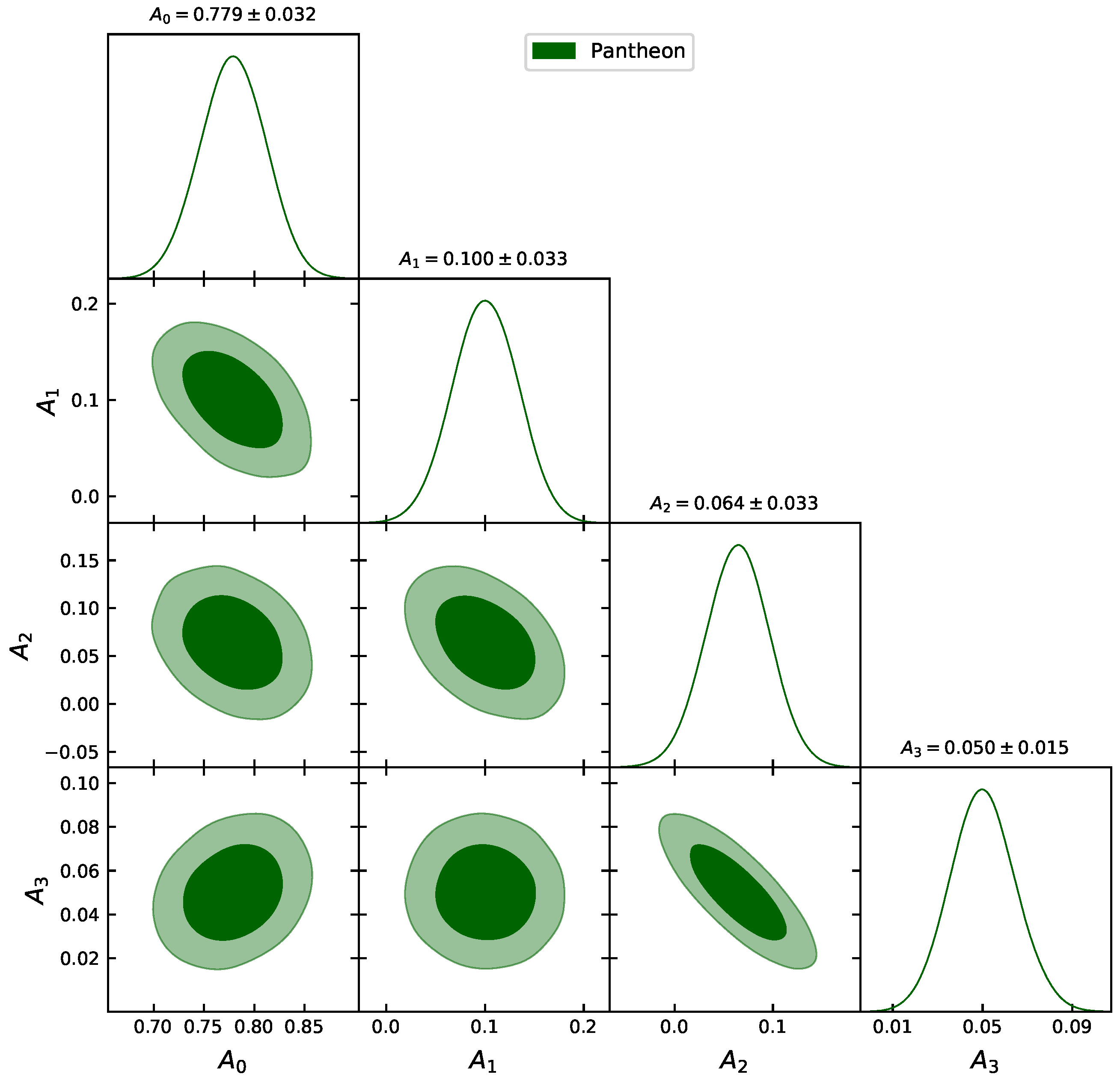
We employ the emcee package in Python for performing a Markov chain Monte Carlo (MCMC) analysis, and provide the best-fit estimates and upper limit of the parameters. We are presented the estimated values of parameters in Table 1.
In Figure 1 and Figure 2, we present the Hubble and Pantheon samples, respectively, with our model. Refer to the triangle plot in Figure 3 and Figure 4 for a complete survey of the parameter space with respect to Hubble and Pantheon data samples; the values are restricted to the positive quadrant as they behave like the density parameters. For further study, we refer to these constrained values of the parameters.
5. Viscous Fluid Models in Gravity
Here, we are going to discuss the cosmological models constructed using the bulk viscous fluid. We also test the energy conditions of viscous fluid models to check their self-stability. We have constructed three models; in the first case, we presume a linear functional form of Q. The motivation behind taking this form is that it recovers the fundamental laws of gravity. Besides this, we discuss the power-law form of Q and logarithmic dependence of models in the second and third cases, respectively.
5.1. Model-1:
In this subsection, we assume the linear functional form of Q with the free parameter . Now, using , we find the following expressions for energy density, pressure, and equation of state parameter, respectively.
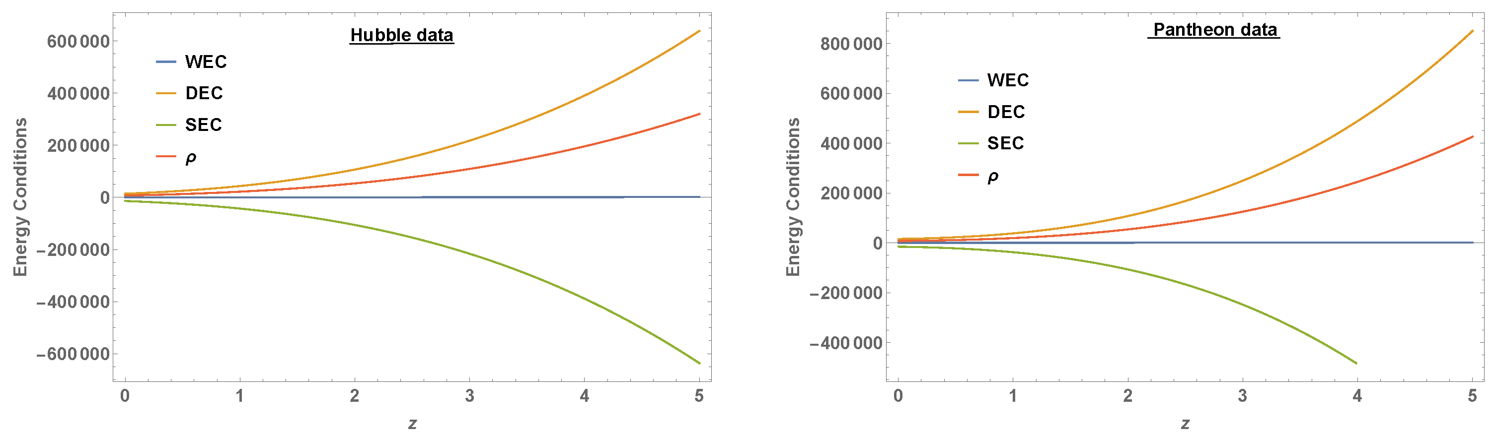
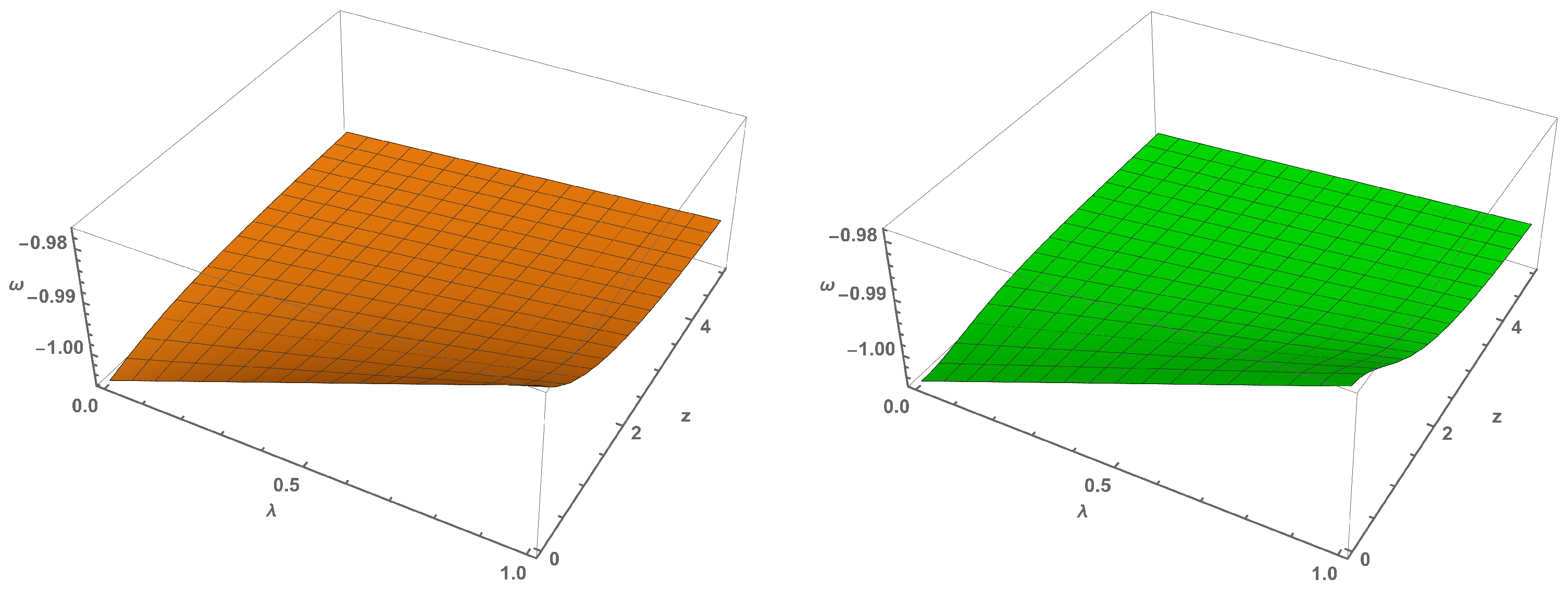
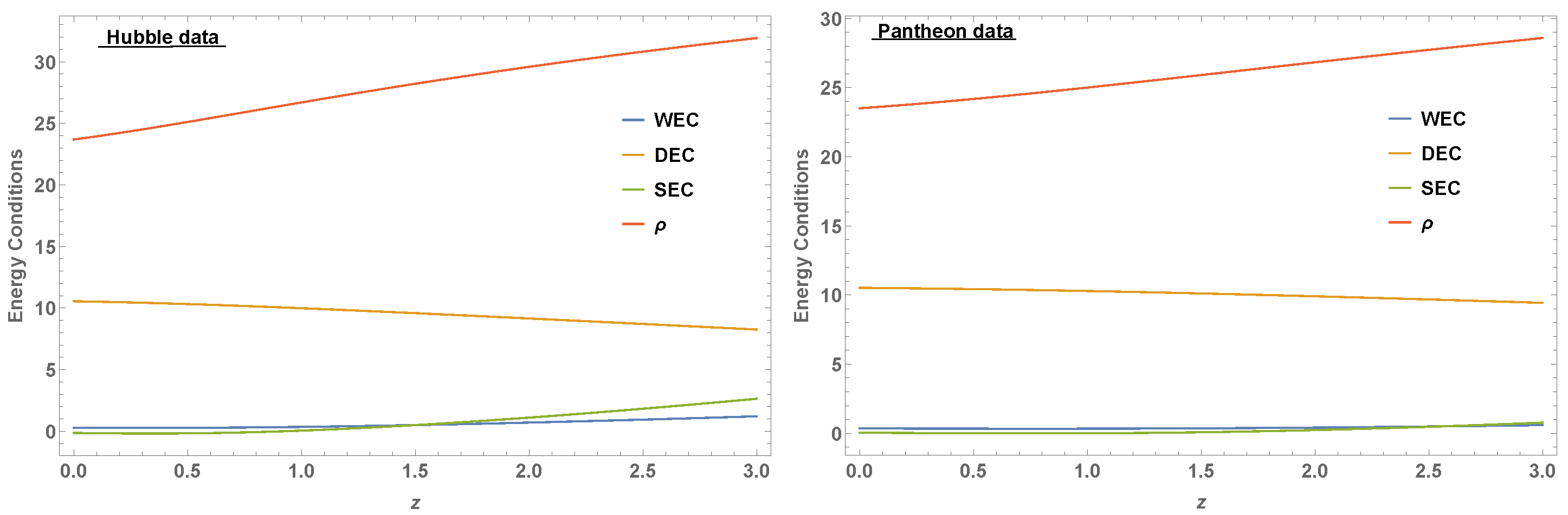
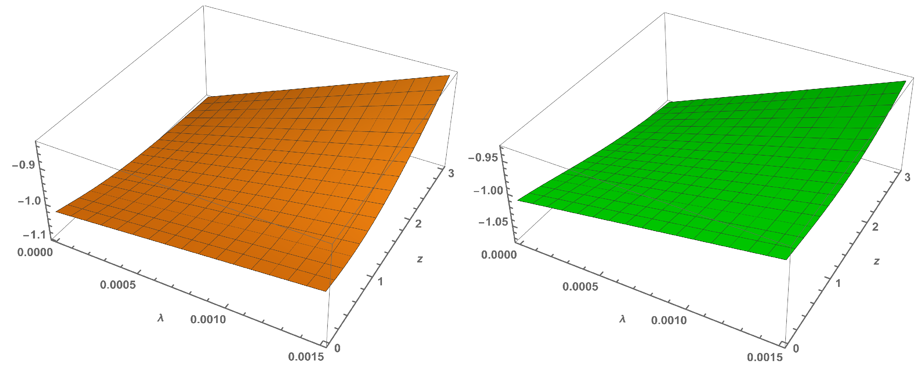
Using (30) and (31) in the energy conditions, we have shown the profiles of energy density, WEC, NEC, DEC, and SEC against redshift z in Figure 5. From that figure, one can clearly observe that all the energy conditions satisfy while the SEC is violated. These are in agreement with the present scenario of the universe. In Figure 6, we have drawn the equation of state parameter behavior concerning the redshift z and . The profile of EoS shows that it takes its values very close to , which aligns with the result of the CDM model. Further, we observed that for negative values of , our model is showing the phantom behavior.
5.2. Model-2:
For the second model, we presume a power-law functional form of Q, where m and n are the free model parameters [8]. For this, the energy density, pressure, and equation of state parameter can be rewritten as
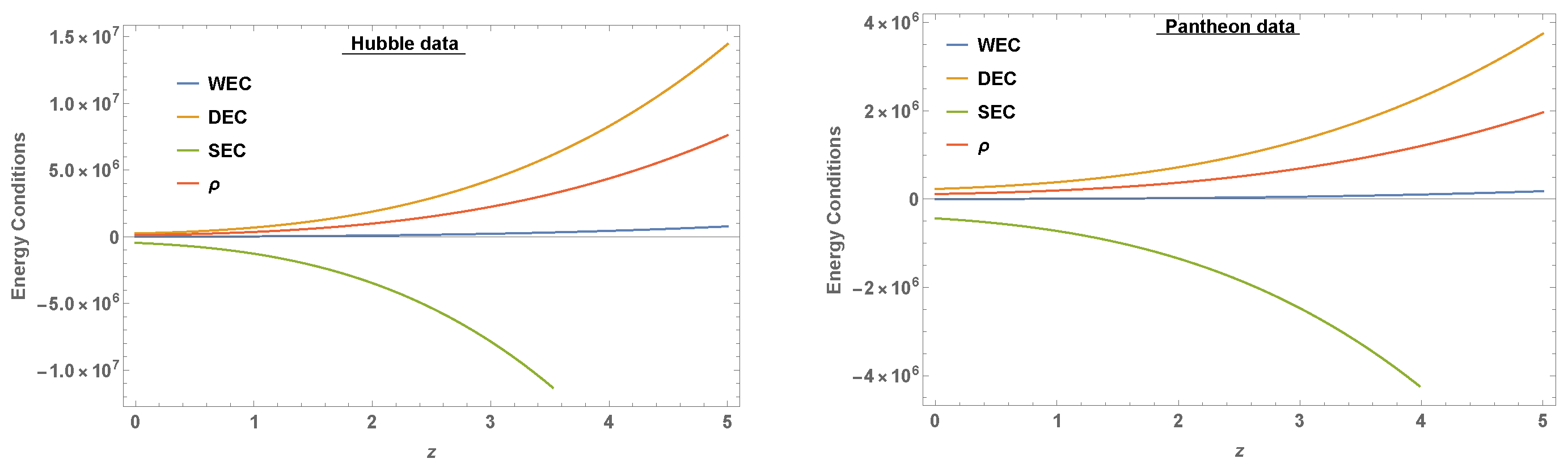
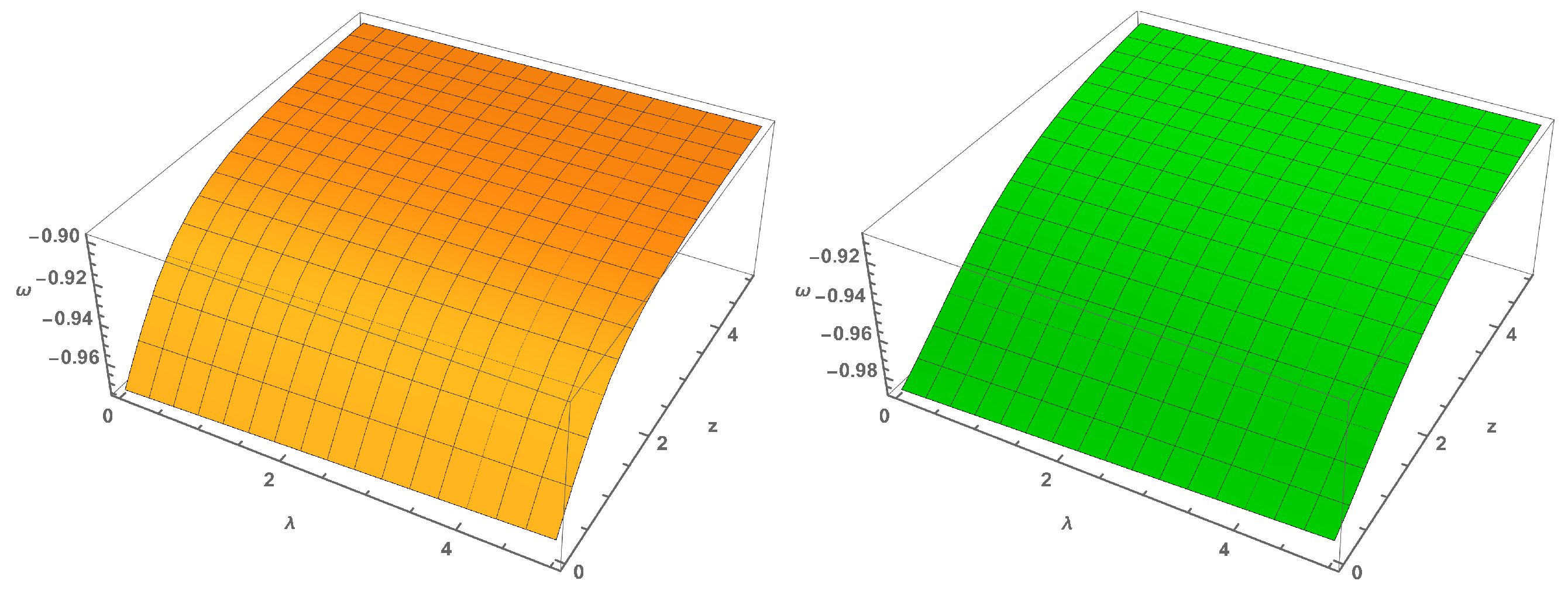
It is well-known that the energy density should be non-negative in order to have a viable cosmological model. So, keeping this in mind and using the constraint values of parameters, we found the relation between m and n as (for Hubble) and (for Pantheon) such that . In Figure 7, the profiles of all the energy conditions have been drawn using (33) and (34) in the above conditions. From those profiles, we conclude that all those behaviors indicate that the accelerated expansion of the universe, i.e., SEC, has been violated, and other energy conditions have been satisfied. The behavior EoS have been shown using (35) in Figure 8. Also, its values lie near to .
5.3. Model-3:
Here, we discuss the logarithmic function of the non-metricity Q with the free parameters and [8]. The energy density, pressure, and equation of state parameter can be written as
Following the same procedure discussed above , we found that (for Hubble) and (for Pantheon). In Figure 9 and Figure 10, the profiles of energy conditions and equation of state parameter have been presented, respectively. For this case, SEC has been violated, and the energy density is positive over the whole range. This result is also an agreement with the accelerated expansion of the universe. The values of are close to .
6. Final Remarks
The recent interests in the universe impel us to go beyond the standard formulation of gravitational interaction, and for this, several modified theories of gravity have been proposed in the literature. However, one of the crucial tasks is to define their self-stability. As is well known, energy conditions are the best tools to test the cosmological models’ self-consistency. The physical motivation to check the energy conditions of a new cosmological model helps us describe its compatibility with the space-time casual and geodesic structure. In this manuscript, we presumed a well motivated Hubble parameter and then constructed the cosmological models by adding bulk viscous fluid in the cosmological fluid within the gravity framework. We have also adopted the parametrization technique to discuss the null, the strong, the weak, and the dominated energy conditions for three types of gravity models. The Hubble dataset and largest Pantheon supernovae dataset were used to constrain the coefficients in the expression for the Hubble parameter.
In our first approach, we have considered a linear function of the non-metricity Q model (). Such a model helps us to deal with the fundamental theories. The profiles presented in Figure 5 reveal the accelerated expansion of the universe. For our second model, we have considered a polynomial function of Q with two free parameters m and n. The self-stability of this model was checked through the energy conditions. From Figure 7, we observed that SEC was violated while other energy conditions are satisfied. For the last model, we have presumed a logarithmic functional form of the non-metricity Q with two free parameters and . The graphics depicted in Figure 8 indicate the universe’s accelerated expansion phase with a specific range of and . Moreover, such a model violates SEC with the positive energy density. These types of results are in good agreement with the current accelerated scenario of the universe.
For the sake of completeness, we derived and discussed the behaviors of equation of state parameter (EoS) for three viscous fluid models. In Figure 6, Figure 8 and Figure 10, the profiles of have been shown for three cases, respectively. From those figures, one can observe that presenting its values very close to −1, which is compatible with the negative pressure of the present scenario of the universe. These results also collaborate with current astronomical observations, as well as the CDM description for dark energy [50]. In addition, we observed that, for all models, the equation of state parameter converges to phantom phase for negative values of viscous fluid parameters .
Further, one can compare the bulk viscosity effect on our three models. In the case of Model-1 and Model-2, any value of bulk viscosity coefficient shows a consistent result with the observation and the current scenario of the universe. Whereas in the case of Model-3, becomes very sensitive. If we consider the value of , then our DEC will be violated. As a result, observed particles move faster than light, which leads to singularity in the present stage. In conclusion, we can say that the viscosity effect is more significant in the case of model-1 and model-2 in comparison to model-3.
The above results allowed us to examine the self-stability of the different families of bulk viscous fluid models in symmetric teleparallel gravity. Also, it sheds light on a new direction of modified theories compatible with recent interests, particularly, the accelerated expansion of the universe. Moreover, it would be interesting to explore the symmetric teleparallel gravity in more generalized viscous fluid models. That may provide us some impressive results. In the near future, we plan to investigate some of the above ideas and hope to report them.
Author Contributions
Conceptualization, S.M.; Data curation, S.M and A.P.; Formal analysis, P.K.S.; Investigation, S.M.; Methodology, S.M.; Project administration, P.K.S.; Software, S.M. and A.P.; Supervision, P.K.S.; Validation, P.K.S.; Visualization, S.M. Writing—original draft, S.M.; Writing—review & editing, A.P. and P.K.S. All authors have read and agreed to the published version of the manuscript.
Funding
This research received no external funding.
Institutional Review Board Statement
Not applicable.
Informed Consent Statement
Not applicable.
Data Availability Statement
There are no new data associated with this article.
Acknowledgments
S.M. acknowledges Department of Science & Technology (DST), Govt. of India, New Delhi, for awarding INSPIRE Fellowship (File No. DST/INSPIRE Fellowship/2018/IF180676). PKS acknowledges CSIR, New Delhi, India for financial support to carry out the Research project [No.03(1454)/19/EMR-II, Dt. 2 August 2019].
Conflicts of Interest
The authors declare no conflict of interest.
References
- Riess, A.G.; Filippenko, A.V.; Challis, P.; Clocchiatti, A.; Diercks, A.; Garnavich, P.M.; Gilliland, R.L.; Hogan, J.C.; Jha, S.; Kirshner, P.R.; et al. Observational Evidence from Supernovae for an Accelerating Universe and a Cosmological Constant. ApJ 1998, 116, 1009. [Google Scholar] [CrossRef] [Green Version]
- Perlmutter, S.; Aldering, G.; Goldhaber, G.; Knop, R.A.; Nugent, P.; Castro, P.G.; Deustua, S.; Fabbro, S.; Goobar, A.; Groom, D.E.; et al. Measurements of Ω and Λ from 42 High-Redshift Supernovae. ApJ 1999, 517, 565. [Google Scholar] [CrossRef]
- Hinshaw, G.; Hinshaw, G.; Larson, D.; Komatsu, E.; Spergel, D.N.; Bennett, C.L.; Dunkley, J.; Nolta, M.R.; Halpern, M.; Hill, R.S.; et al. Nine-Year Wilkinson Microwave Anisotropy Probe (Wmap) Observations: Cosmological Parameter Results. ApJ 2013, 208, 19. [Google Scholar] [CrossRef] [Green Version]
- Suzuki, N.; Rubin, D.; Lidman, C.; Aldering, G.; Amanullah, R.; Barbary, K.; Barrientos, L.F.; Botyanszki, J.; Brodwin, M.; Connolly, N.; et al. The Hubble Space Telescope Cluster Supernova Survey. V. Improving the Dark-Energy Constraints Above z > 1 and Building an Early-Type-Hosted Supernova Sample. ApJ 2012, 746, 85. [Google Scholar] [CrossRef] [Green Version]
- Carlip, S. Hiding the Cosmological Constant. Phys. Rev. Lett. 2019, 123, 131302. [Google Scholar] [CrossRef] [Green Version]
- Jimenez, J.B.; Heisenberg, L.; Koivisto, T. Coincident general relativity. Phys. Rev. D 2018, 98, 044048. [Google Scholar] [CrossRef] [Green Version]
- Lazkoz, R.; Lobo, F.S.N.; Ortiz-Baños, M.; Salzano, V. Observational constraints of f(Q) gravity. Phys. Rev. D 2019, 100, 104027. [Google Scholar] [CrossRef] [Green Version]
- Mandal, S.; Sahoo, P.K.; Santos, J.R.L. Energy conditions in f(Q) gravity. Phys. Rev. D 2020, 102, 024057. [Google Scholar] [CrossRef]
- Mandal, S.; Wang, D.; Sahoo, P.K. Cosmography in f(Q) gravity. Phys. Rev. D 2020, 102, 124029. [Google Scholar] [CrossRef]
- Harko, T.; Koivisto, T.S.; Lobo, F.S.N.; Olmo, G.J.; Rubiera-Garcia, D. Coupling matter in modified Q gravity. Phys. Rev. D 2018, 98, 084043. [Google Scholar] [CrossRef] [Green Version]
- Barros, B.J.; Barreiro, T.; Koivisto, T.; Nunes, N.J. Testing F (Q) gravity with redshift space distortions. Phys. Dark Universe 2020, 30, 100616. [Google Scholar] [CrossRef]
- Jimenez, J.B.; Heisenberg, L.; Koivisto, T.; Pekar, S. Cosmology in f(Q) geometry. Phys. Rev. D 2020, 101, 103507. [Google Scholar] [CrossRef]
- Hasan, Z.; Mandal, S.; Sahoo, P.K. Traversable Wormhole Geometries in f(Q) Gravity. Fortschritte Der Phys. 2021, 69, 2100023. [Google Scholar] [CrossRef]
- Solanki, R.; Mandal, S.; Sahoo, P.K. Cosmic acceleration with bulk viscosity in modified f(Q) gravity. Phys. Dark Universe 2021, 32, 100820. [Google Scholar] [CrossRef]
- Eckart, C. The Thermodynamics of Irreversible Processes. III. Relativistic Theory of the Simple Fluid. Phys. Rev. 1940, 58, 919. [Google Scholar] [CrossRef]
- Weinberg, S. Entropy Generation and the Survival of Protogalaxies in an Expanding Universe. Astrophys. J. 1971, 168, 175. [Google Scholar] [CrossRef]
- Treciokas, R.; Ellis, G.F.R. Isotropic solutions of the Einstein-Boltzmann equations. Commun. Math. Phys. 1971, 23, 1–22. [Google Scholar] [CrossRef]
- Misner, C.W. The Isotropy of the Universe. Astrophys. J. 1968, 151, 431. [Google Scholar] [CrossRef]
- Israel, W.; Vardalas, J.N. Transport coefficients of a relativistic quantum gas. Nuovo C. Lett. 1970, 4, 887. [Google Scholar] [CrossRef]
- Murphy, G.L. Big-Bang Model Without Singularities. Phys. Rev. D 1973, 8, 4231. [Google Scholar] [CrossRef]
- Belinskii, V.A.; Kalatnikov, I.M. On the effect of viscosity on the character of the cosmological singularity. Pisma Zh. Eksp. Tekhn. Fiz. 1974, 21, 223. [Google Scholar]
- Hu, M.-G.; Meng, X.-H. Bulk viscous cosmology: Statefinder and entropy. Phys. Lett. B 2006, 635, 186. [Google Scholar] [CrossRef]
- Ren, J.; Meng, X.-H. Cosmological model with viscosity media (dark fluid) described by an effective equation of state. Phys. Lett. B 2006, 633, 1. [Google Scholar] [CrossRef] [Green Version]
- Ren, J.; Meng, X.-H. Modified equation of state, scalar field, and bulk viscosity in Friedmann universe. Phys. Lett. B 2006, 636, 5. [Google Scholar] [CrossRef] [Green Version]
- Gagnon, J.S.; Lesgourgues, J. Dark goo: Bulk viscosity as an alternative to dark energy. J. Cosmol. Astropart. Phys. 2011, 9, 026. [Google Scholar] [CrossRef] [Green Version]
- Diosi, L.; Keszthelyi, B.; Lukacs, B.; Paal, G. Viscosity and the monopole density of the Universe. Acta Phys. Pol. B 1984, 15, 909. [Google Scholar]
- Waga, I.; Falcao, R.C.; Chanda, R. Bulk-viscosity-driven inflationary model. Phys. Rev. D 1986, 15, 1839. [Google Scholar] [CrossRef]
- Barrow, J.D. The deflationary universe: An instability of the de Sitter universe. Phys. Lett. 1986, 180, 335. [Google Scholar] [CrossRef]
- Barrow, J.D. String-driven inflationary and deflationary cosmological models. Nucl. Phys. B 1988, 380, 743. [Google Scholar] [CrossRef]
- Bemfica, F.S.; Disconzi, M.M.; Noronha, J. Causality of the Einstein-Israel-Stewart Theory with Bulk Viscosity. Phys. Rev. Lett. 2019, 122, 221602. [Google Scholar] [CrossRef] [Green Version]
- Chattopadhyay, S. Israel-Stewart Approach to Viscous Dissipative Extended Holographic Ricci Dark Energy Dominated Universe. Adv. High Energy Phys. 2016, 2016, 8515967. [Google Scholar] [CrossRef]
- Olson, T.S. Stability and causality in the Israel-Stewart energy frame theory. Ann. Phys. 1990, 199, 1. [Google Scholar] [CrossRef]
- Ilg, P.; Ottinger, H.C. Nonequilibrium relativistic thermodynamics in bulk viscous cosmology. Phys. Rev. D 1999, 61, 023510. [Google Scholar] [CrossRef]
- Wilson, J.R.; Mathews, G.J.; Fuller, G.M. Bulk viscosity, decaying dark matter, and the cosmic acceleration. Phys. Rev. D 2007, 75, 043521. [Google Scholar] [CrossRef] [Green Version]
- Xu, Y.D.; Huang, Z.G.; Zhai, X.H. Generalized Chaplygin gas model with or without viscosity in the w-w′ plane. Astrophys. Space Sci. 2012, 337, 493. [Google Scholar] [CrossRef]
- Feng, C.J.; Li, X.Z. Viscous Ricci dark energy. Phys. Lett. B 2009, 680, 355. [Google Scholar] [CrossRef] [Green Version]
- Capozziello, S.; Cardone, V.F.; Elizalde, E.; Nojiri, S.; Odintsov, S.D. Observational constraints on dark energy with generalized equations of state. Phys. Rev. D 2006, 73, 043512. [Google Scholar] [CrossRef] [Green Version]
- Mohan, N.D.J.; Sasidharan, A.; Mathew, T.K. Bulk viscous matter and recent acceleration of the universe based on causal viscous theory. Eur. Phys. J. C 2017, 77, 849. [Google Scholar] [CrossRef]
- Velten, H.; Schwarz, D.J. Dissipation of dark matter. Phys. Rev. D 2012, 86, 083501. [Google Scholar] [CrossRef] [Green Version]
- Cataldo, M.; Cruz, N.; Lepe, S. Viscous dark energy and phantom evolution. Phys. Lett. B 2005, 619, 5. [Google Scholar] [CrossRef] [Green Version]
- Arora, S.; Meng, X.-H.; Pacif, S.K.J.; Sahoo, P.K. Effective equation of state in modified gravity and observational constraints. Class. Quant. Grav. 2020, 30, 205022. [Google Scholar] [CrossRef]
- Cardenas, V.H.; Cruz, M.; Lepe, S. Cosmic expansion with matter creation and bulk viscosity. Phys. Rev. D 2020, 102, 123543. [Google Scholar] [CrossRef]
- Raychaudhuri, A. Relativistic Cosmology. I. Phys. Rev. D 1955, 98, 1123. [Google Scholar] [CrossRef]
- Nojiri, S.; Odintsov, S.D. Introduction to Modified Gravity and Gravitational Alternative for Dark Energy. Int. J. Geom. Methods Mod. Phys. 2007, 4, 115. [Google Scholar] [CrossRef] [Green Version]
- Ehlers, J. AK Raychaudhuri and His Equation. IJMPD 2006, 15, 1573. [Google Scholar] [CrossRef] [Green Version]
- Arora, S.; Santos, J.R.L.; Sahoo, P.K. Constraining f(Q, T) gravity from energy conditions. Phys. Dark Universe 2021, 31, 100790. [Google Scholar] [CrossRef]
- Capozziello, S.; Nojiri, S.; Odintsov, S.D. The role of energy conditions in f(R) cosmology. Phys. Lett. B 2018, 781, 99. [Google Scholar] [CrossRef]
- Saini, T.D.; Raychaudhury, S.; Sahni, V.; Starobinsky, A.A. Reconstructing the Cosmic Equation of State from Supernova Distances. Phys. Rev. Lett. 2000, 85, 1162. [Google Scholar] [CrossRef] [PubMed] [Green Version]
- Capozziello, S.; Cardone, V.F.; Troisi, A. Reconciling dark energy models with f(R) theories. Phys. Rev. D 2005, 71, 043503. [Google Scholar] [CrossRef]
- Planck Collaboration. Planck 2018 results—VI. Cosmological parameters. A&A 2020, 641, 67. [Google Scholar]
- Sahni, V.; Saini, T.D.; Starobinsky, A.A.; Alam, U. Statefinder—A new geometrical diagnostic of dark energy. JETP Lett. 2003, 77, 201. [Google Scholar] [CrossRef]
- Pourbagher, A.; Amani, A. Thermodynamics and stability of f(T, B) gravity with viscous fluid by observational constraints. Astrophys. Space Sci. 2019, 364, 140. [Google Scholar] [CrossRef] [Green Version]
- Sharov, G.S.; Vasiliev, V.O. How predictions of cosmological models depend on Hubble parameter data sets. Math. Model. Geom. 2018, 6, 1. [Google Scholar] [CrossRef]
- Chuang, C.H.; Wang, Y. Modelling the anisotropic two-point galaxy correlation function on small scales and single-probe measurements of H(z), DA(z) and f(z) σ8(z) from the Sloan Digital Sky Survey DR7 luminous red galaxies. Mon. Not. R. Astron. Soc. 2013, 435, 255. [Google Scholar] [CrossRef] [Green Version]
- Chuang, C.-H.; Prada, F.; Cuesta, A.J.; Eisenstein, D.J.; Kazin, E.; Padmanabhan, N.; Sánchez, A.G.; Xu, X.; Beutler, F.; Manera, M.; et al. The clustering of galaxies in the SDSS-III Baryon Oscillation Spectroscopic Survey: Single-probe measurements and the strong power of f(z)σ8(z) on constraining dark energy. Mon. Not. R. Astron. Soc. 2013, 433, 3559. [Google Scholar] [CrossRef]
- Delubac, T.; Bautista, J.E.; Busca, N.G.; Rich, J.; Kirkby, D.; Bailey, S.; Font-Ribera, A.; Slosar, A.; Lee, K.-G.; Pieri, M.M.; et al. Baryon acoustic oscillations in the Lyα forest of BOSS DR11 quasars. Astron. Astrophys. 2015, 574, 17. [Google Scholar] [CrossRef] [Green Version]
- Anderson, L.; Aubourg, E.; Bailey, S.; Beutler, F.; Bhardwaj, V.; Blanton, M.; Bolton, A.S.; Brinkmann, J.; Brownstein, J.R.; Burden, A.; et al. The clustering of galaxies in the SDSS-III Baryon Oscillation Spectroscopic Survey: Baryon acoustic oscillations in the Data Releases 10 and 11 Galaxy samples. Mon. Not. R. Astron. Soc. 2014, 441, 24. [Google Scholar] [CrossRef] [Green Version]
- Alam, S.; Ata, M.; Bailey, S.; Beutler, F.; Bizyaev, D.; Blazek, J.A.; Bolton, A.S.; Brownstein, J.R.; Burden, A.; Chuang, C.-H.; et al. The clustering of galaxies in the completed SDSS-III Baryon Oscillation Spectroscopic Survey: Cosmological analysis of the DR12 galaxy sample. Mon. Not. R. Astron. Soc. 2017, 470, 2617. [Google Scholar] [CrossRef] [Green Version]
- Simon, J.; Verde, L.; Jimenez, R. Constraints on the redshift dependence of the dark energy potential. Phys. Rev. D 2005, 71, 123001. [Google Scholar] [CrossRef] [Green Version]
- Stern, D.; Jimenez, R.; Verde, L.; Kamionkowski, M.; Stanford, S.A. Cosmic chronometers: Constraining the equation of state of dark energy. I: H(z) measurements. JCAP 2010, 02, 008. [Google Scholar] [CrossRef] [Green Version]
- Moresco, M. Raising the bar: New constraints on the Hubble parameter with cosmic chronometers at z ∼ 2. Mon. Not. R. Astron. Soc. Lett. 2015, 450, L16. [Google Scholar] [CrossRef] [Green Version]
- Ratsimbazafy, A.L.; Loubser, S.I.; Crawford, S.M.; Cress, C.M.; Bassett, B.A.; Nichol, R.C.; Vaisanen, P. Age-dating luminous red galaxies observed with the Southern African Large Telescope. Mon. Not. R. Astron. Soc. 2017, 467, 3239. [Google Scholar] [CrossRef] [Green Version]
- Scolnic, D.M.; Jones, D.O.; Rest, A.; Pan, Y.C.; Chornock, R.; Foley, R.J.; Huber, M.E.; Kessler, R.; Narayan, G.; Riess, A.G.; et al. The Complete Light-curve Sample of Spectroscopically Confirmed SNe Ia from Pan-STARRS1 and Cosmological Constraints from the Combined Pantheon Sample. ApJ 2018, 859, 101. [Google Scholar] [CrossRef]
Figure 1.
The evolution of Hubble parameter with respect to redshift z is shown here. The red line represents our model (i.e., the profile of as presented in (26)) and dashed-line indicates the CMD model with and . The dots are shown on the Hubble dataset with the error bar.
Figure 1.
The evolution of Hubble parameter with respect to redshift z is shown here. The red line represents our model (i.e., the profile of as presented in (26)) and dashed-line indicates the CMD model with and . The dots are shown on the Hubble dataset with the error bar.

Figure 2.
The evolution of with respect to redshift z is shown here. The red line represents our model (i.e., the profile of as presented in (26)) and dashed-line indicates the CMD model with and . The dots are shown in the 1048 Pantheon dataset with the error bar.
Figure 2.
The evolution of with respect to redshift z is shown here. The red line represents our model (i.e., the profile of as presented in (26)) and dashed-line indicates the CMD model with and . The dots are shown in the 1048 Pantheon dataset with the error bar.

Figure 3.
The marginalized constraints on the coefficients in the expression of Hubble parameter in Equation (26) are shown by using the Hubble sample.
Figure 3.
The marginalized constraints on the coefficients in the expression of Hubble parameter in Equation (26) are shown by using the Hubble sample.

Figure 4.
The marginalized constraints on the coefficients in the expression of Hubble parameter in Equation (26) are shown by using the Pantheon SNe Ia sample.
Figure 4.
The marginalized constraints on the coefficients in the expression of Hubble parameter in Equation (26) are shown by using the Pantheon SNe Ia sample.

Figure 5.
The behavior of energy conditions against the redshift parameter z with the constraint values of the coefficients in (29) and for .
Figure 5.
The behavior of energy conditions against the redshift parameter z with the constraint values of the coefficients in (29) and for .

Figure 6.
The behavior of EoS parameter against the redshift parameter z and with the constraint values of the coefficients in (29) and for . Left side graph for Hubble data and right side graph for Pantheon data.
Figure 6.
The behavior of EoS parameter against the redshift parameter z and with the constraint values of the coefficients in (29) and for . Left side graph for Hubble data and right side graph for Pantheon data.

Figure 7.
The behavior of energy conditions against the redshift parameter z with the constraint values of the coefficients in (29) for .
Figure 7.
The behavior of energy conditions against the redshift parameter z with the constraint values of the coefficients in (29) for .

Figure 8.
The behavior of EoS parameter against the redshift parameter z and with the constraint values of the coefficients in (29) and for . Left side graph for Hubble data and right side graph for Pantheon data.
Figure 8.
The behavior of EoS parameter against the redshift parameter z and with the constraint values of the coefficients in (29) and for . Left side graph for Hubble data and right side graph for Pantheon data.

Figure 9.
The behavior of energy conditions against the redshift parameter z with the constraint values of the coefficients in (29), for , and .
Figure 9.
The behavior of energy conditions against the redshift parameter z with the constraint values of the coefficients in (29), for , and .

Figure 10.
The behavior of the EoS parameter against the redshift parameter z and with the constraint values of the coefficients in (29) and for . Left side graph for Hubble data and right side graph for Pantheon data.
Figure 10.
The behavior of the EoS parameter against the redshift parameter z and with the constraint values of the coefficients in (29) and for . Left side graph for Hubble data and right side graph for Pantheon data.


Table 1.
The marginalized constraining results on four model parameters are shown by using the Hubble and Pantheon SNe Ia sample.
Table 1.
The marginalized constraining results on four model parameters are shown by using the Hubble and Pantheon SNe Ia sample.
| Dataset | H(z) Dataset | Pantheon Dataset |
|---|---|---|
Publisher’s Note: MDPI stays neutral with regard to jurisdictional claims in published maps and institutional affiliations. |
© 2022 by the authors. Licensee MDPI, Basel, Switzerland. This article is an open access article distributed under the terms and conditions of the Creative Commons Attribution (CC BY) license (https://creativecommons.org/licenses/by/4.0/).
Share and Cite
MDPI and ACS Style
Mandal, S.; Parida, A.; Sahoo, P.K. Observational Constraints and Some Toy Models in f(Q) Gravity with Bulk Viscous Fluid. Universe 2022, 8, 240. https://0-doi-org.brum.beds.ac.uk/10.3390/universe8040240
AMA Style
Mandal S, Parida A, Sahoo PK. Observational Constraints and Some Toy Models in f(Q) Gravity with Bulk Viscous Fluid. Universe. 2022; 8(4):240. https://0-doi-org.brum.beds.ac.uk/10.3390/universe8040240
Chicago/Turabian StyleMandal, Sanjay, Abhishek Parida, and Pradyumn Kumar Sahoo. 2022. "Observational Constraints and Some Toy Models in f(Q) Gravity with Bulk Viscous Fluid" Universe 8, no. 4: 240. https://0-doi-org.brum.beds.ac.uk/10.3390/universe8040240
Note that from the first issue of 2016, this journal uses article numbers instead of page numbers. See further details here.