Spatial Distribution and Mechanism of Urban Occupation Mixture in Guangzhou: An Optimized GeoDetector-Based Index to Compare Individual and Interactive Effects

Abstract

Numerous studies have been devoted to uncovering the characteristics of resident density and urban mobility with multisource geospatial big data. However, little attention has been paid to the internal diversity of residents such as their occupations, which is a crucial aspect of urban vibrancy. This study aims to investigate the variation between individual and interactive influences of built environment factors on occupation mixture index (OMI) with a novel GeoDetector-based indicator. This study first integrated application (App) use and mobility patterns from cellphone data to portray residents’ occupations and evaluate the OMI in Guangzhou. Then, the mechanism of OMI distribution was analyzed with the GeoDetector model. Next, an optimized GeoDetector-based index, interactive effect variation ratio (IEVR) was proposed to quantify the variation between individual and interactive effects of factors. The results showed that land use mixture was the dominating factor, and that land use mixture, building density, floor area ratio, road density affected the OMI distribution directly. Some interesting findings were uncovered by IEVR. The influences of cultural inclusiveness and metro accessibility were less important in factor detector result, while they were found to be the most influential in an indirect way interacting with other built environment factors. The results suggested that both “hardware facilities” (land use mixture, accessibility) and “soft facilities” (cultural inclusiveness) should be considered in planning a harmonious urban employment space and sustainable city.

1. Introduction

The continuous development of urbanization has been making the city increasingly crowded, especially in metropolises [1,2,3]. Understanding the spatial distribution of urban population density is necessary and beneficial in many aspects for a city including urban traffic planning, public facilities planning and the identification of urban functional areas and buildings [4,5,6,7,8,9]. Employed people from all walks of life are one of the most significant components of urban population. For example, the spatial structure of workspaces, jobs-housing balance and commuting behavior can be explored for urban planning and management based on the found distribution as well as the classification of the employed population density [10,11,12,13].

Currently, the rapid development and wide applications of geospatial big data have greatly contributed to the literature in human behavior, spatio-temporal mobility and population distribution, such as ridesourcing and taxi trip records [14,15,16], smart cards dataset [17,18,19], bike sharing GPS records [20,21,22,23,24], cellphone dataset [25,26] and social media data [27,28,29,30,31,32]. Numerous studies have been conducted and have found that diversity was one of the most important characteristics of residents’ density distribution and mobility patterns [4]. For instance, residents’ distribution and mobility patterns vary from working days to off days [33], from working time to off time during weekday, and even in a short period of time [34,35,36]. Li et al., analyzed the spatio-temporal dynamic of urban population density distribution with Baidu heat map data in Xian at multi time scales: morning, afternoon, evening and nighttime, and the mechanism of the dynamic was also explored with regression models [4]. Wu et al., explored the hourly urban vibrancy and the influencing factors with check-in data in Shenzhen by geographically and temporally weighted regression [37]. Tu et al., proposed a framework integrating cellphone data, POIs (point of interests) and check-in data to portray urban vibrancy in Shenzhen, and its mechanism was explored with global and local regressions [38]. Guo et al., evaluated the dynamic vitality on the street scale at different times with POIs and cellphone data in Xining [39]. Meng et al., explored the association between urban vibrancy and landscape characteristics with review data via a regression model in Shenzhen [40]. Fu et al., measured the urban vibrancy with real-time population distribution data and small catering business data, and its mechanism was explored with a geographically weighted regression model in Urumqi [41]. Generally, occupation is the basic diversity and classification of residents, and residents from all walks of life together form the society and city [10]. Most related studies focused on the diversity of residents’ spatio-temporal characteristics, however, little attention was paid to the internal diversity of residents themselves, which is also an indispensable aspect of urban vibrancy.

A late study has developed the framework of portrait identification with cellphone big data and found that high OMI was observed in and around the CBD [10]. However, the potential driving factors of OMI distribution still remained unknown. Based on the literature, the high OMI in the CBD might result from it being the economic and social nerve center of the city with the predominance of commercial activities [42]. Furthermore, areas with a higher level of urbanization are more advantageous with more developed markets and better access to consumer goods, more resources and affluence, and thus stimulating the economic development of all walks of life [43,44,45,46]. In conclusion, a city center is beneficial to the economic development and the residents from various occupations in multiple aspects. Therefore, the driving mechanism of OMI distribution of a city, especially CBD, should be explored quantitatively.

Methodologically, numerous models have been applied to investigate the mechanism of population density distribution or urban vibrancy including spatial (geographically weighted regression [37,38,40,47], geographically and temporally weighted regression [37] and spatial filtering model [48]) and non-spatial models (multiple linear regression [4]), by which only individual influence of each potential driving factor can be detected. However, the mechanism of a geographical phenomenon (residents’ spatio-temporal distribution in this study) is comprehensive and complex, this is, it is not caused by a single aspect [21]. Therefore, few existing studies were able to analyze the coupling or interactive effects between factors [37,38,39,40,41], which was essential to the exploration of the mechanism. A popular quantitative mechanism uncovering technique called geographical detector model (GeoDetector) was adopted in this study to explore the individual influences and interactive effects of potential driving factors [49,50,51,52]. Previous studies with the GeoDetector model analyzed the individual and interactive influences of variables separately, although few of them were capable to quantitatively evaluate the variation between the individual influence of each variable and its interactive effects with other factors.

To fill the research gaps above, this study aims to explore the spatial distribution and the mechanism of occupation mixture index (OMI) evaluated with cellphone big data in Guangzhou. First, cellphone users’ spatio-temporal characteristics and their frequently used Apps were integrated to portray residents’ occupations. Based on that, the spatial distribution of OMI of the city was calculated and mapped. Second, the mechanism of OMI was analyzed with the GeoDetector model (factor detector and interactive detector sub models). To further compare the variation between the individual effect of each factor and interactive effect of each factors pair, the interactive effect variation ratio (IEVR) was proposed in this study. In the mechanism study, experience from previous studies, data availability and regional characteristics of the study area were taken into account to select the potential driving factors such as cultural inclusiveness measured by cuisines POIs. The framework of the study was shown as Figure 1.

The rest of the paper is structured as follows. Data and methods are introduced in Section 2. Section 3 presents the results and discussion. Section 4 presents the main conclusions.

2. Data and Methods

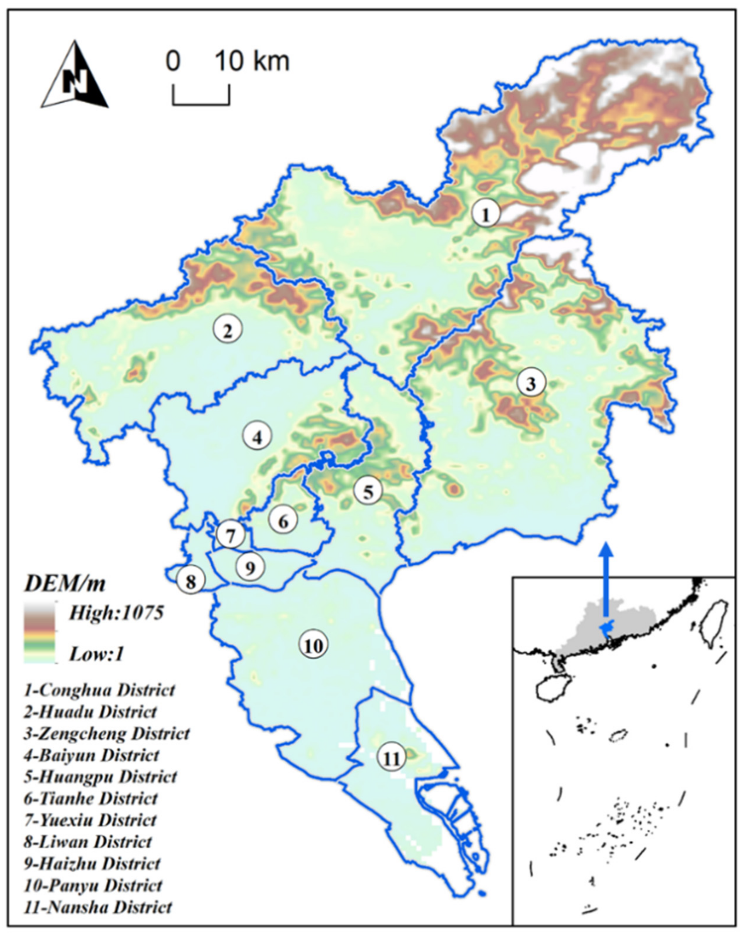
2.1. Study Area

Guangzhou (Figure 2) is the capital of Guangdong Province and one of the megacities in China. It has 11 districts under its jurisdiction, with a total area of 7434.40 square km, which is one of the core cities in Guangdong–Hong Kong–Macao Greater Bay Area. According to the bulletin of the seventh national census of Guangdong Province, the number of permanent residents in Guangzhou reached 18.67 million in 2020, accounting for 14.82% of the total population of the province, ranking first in the province. Moreover, Guangzhou has a long history of opening to the outside world and economic development, forming an open and inclusive multi-cultural urban environment.

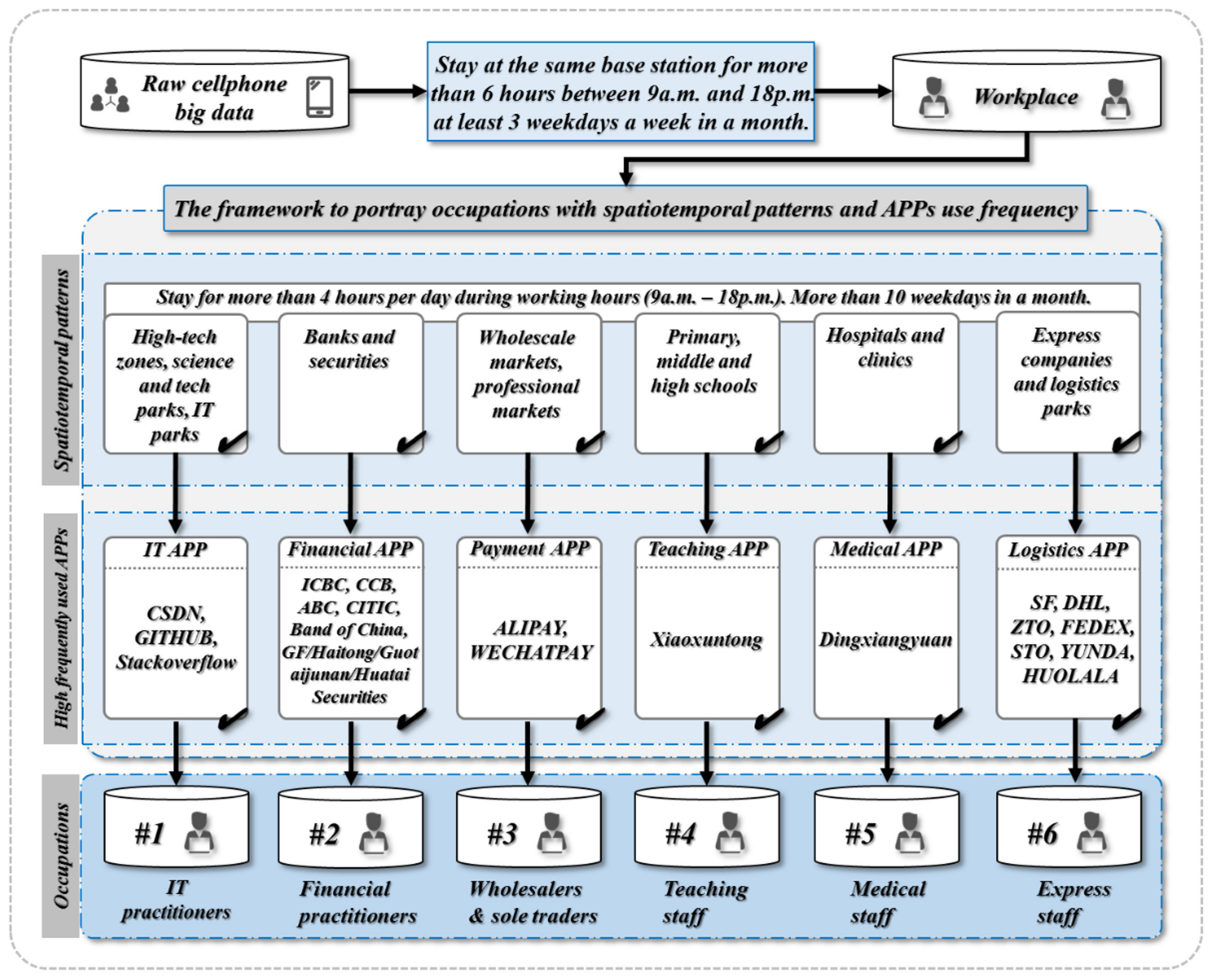
2.2. Cellphone Big Data and Processing Algorithm

The cellphone dataset applied in this study (from 1 November 2020 to 30 November 2020) were provided by a local telecom operator company with the most share of user market. It is noted that the COVID-19 had very little influence on the cellphone dataset since that the COVID-19 blockade policy has stopped and China’s production and life has returned to normal. The cellphone dataset used in this study consists of two parts: the signaling dataset and the Apps use record dataset. It should be noticed that all of the cellphone data in this study were anonymous and aggregated into a 1 km grid cell by the telecom company to protect personal privacy.

The first part is the signaling dataset, which automatically records users’ geographical location and signals when they make phone calls, send/receive messages, turn on/off the phone, use online Apps, etc. (as long as their phones are turned on). According to the work by Zhong et al., turning phones off has little influence on cellphone-data-related studies because it happens occasionally [53]. The original signaling dataset were saved in the Hive (Hadoop-based) database of the telecom operator company. The movement trajectory of users was generated based on their spatio-temporal recorded locations by the telecom operator. Errors such as overlong jump and unnecessary movement were filtered [53]. The operator company provided users’ spatio-temporal location movement list to researchers with a time interval of 30 min due to the time intervals of raw data acquisition. That is, the raw data acquisition frequency ranged from 7 s to 1 day. The data acquired with an interval of 7 s accounted for 1.2%, whereas 92.4% of data were collected within 30 min. Therefore, the data obtained within 30 min were filtered as valid data in this study. Researchers further defined the algorithm to extract work population as follows. First, to record the movement trajectory of users, stay and move were defined as follows. According to the work by Zhong et al., if a user stops at a same location over an hour, it is defined as a stay [53]. And a move is defined when a user’s stop time is less than an hour [53]. That is, trips between two stays are regarded as moves. Second, workplaces of users were extracted by the most frequently staying grid (over 3 weekdays a week during a month) at typical work-time (9 a.m.—18 p.m.) (Figure 2).

The second part is Apps use record dataset, recording the information of each user’ daily visit duration of online Apps. By classifying the Apps into different occupations/industries, each user’ daily Apps use preference can be figured out, which was applied in user’s occupation portrait. The occupation portrait algorithm of the work by Zhang et al. [10] was used in our study to identify six common occupations: IT practitioners, financial practitioners, wholesalers and sole traders, teaching staff, medical staff, and express staff. In general, the occupation portrait algorithm was based on users’ spatio-temporal mobility patterns and Apps daily use duration (Figure 3) [10]. For example, first, a user’s most frequently used Apps belong to IT Apps category (such as CSDN, Github) in a month (social network and recreational Apps like WeChat, QQ, Weibo, Douyin, etc., were excluded to avoid deviation). Second, the user connected the signal tower which is near IT workplace POIs (such as IT park, within 100 m) more than 4 h during work-time of weekday, and more than 10 weekdays in a month. By filtering users with the above algorithm, an IT practitioner was identified in this study [10].

2.3. Occupations Mixure Index

The occupation mixture index (OMI) was measured by Shannon entropy as Equation (1) [10].

$$OMI=-{\sum }_{i=1}^N{p}_i{\log }_n{p}_i$$

(1)

where OMI refers to the value of occupations mixture index; $p_i$ represents the percentage of the $i\mathrm{th}$ type of occupation; n represents the number of occupation types [10].

2.4. Geographical Detector Model

The geographical detector model proposed by Wang et al., is capable of exploring both individual and interactive effects of potential driving factors on the spatial distribution of the dependent variable based on the theory of spatial variance [49,50,51]. Due to the advantage, it has been applied in numerous geographical studies [49,50,51,52], and so on. The geographical detector model consists of four sub-models: factor detector, interactive detector and risk detector as well as ecological detector. Among them, the factor detector and interactive detector are more popular, which were also used in the study to explore the individual and interactive effects of determinants on the occupation mixture index distribution.

2.4.1. The Factor Detector Model (Individual Effect of Factors)

The function of factor detector is to calculate the power determinant (PD) value to quantify the impact of potential determinants on the dependent variable (OMI distribution). In this study, PD value is defined as the difference between one and the ratio of accumulated dispersion variance of the OMI distribution over each sub region to that of over the entire study region [49], which is calculated as Equations (2)–(4).

$$PD=1-\frac{{\sum }_{h=1}^L{N}_h{\sigma }_h^2}{N_{{\sigma }^2}}=1-\frac{SSW}{SST}$$

(2)

$$SSW={\displaystyle \sum }_{h=1}^L{N}_h{\sigma }_h^2$$

(3)

$$SST=N_{{\sigma }^2}$$

(4)

where N refers that a study area consists of N units, which is stratified into h = 1, 2, …, L stratum; and stratum h consists of $N_h$ units; ${\sigma }^2$and ${\sigma }_h^2$ denote the global variance of dependent variable of the study area and the variance of dependent variable in the sub-areas; SSW and SST denote within sum of squares and total sum of squares [49]. The value of PD lies between 0 and 1. A higher PD value means the determinant has a stronger contribution to the OMI distribution. In this study, PD values indicate the consistency of the spatial patterns between the OMI distribution and its potential driving factors [49].

2.4.2. The Interactive Detector Model (Interactive Effect of Factors)

The interaction detector determined whether two individual factors enhance or weaken each other by comparing their combined contribution, as well as their independent contributions [49]. The model classifies the interactive relationship between two factors into seven types as Equation (5) [49]:

$$\begin{array}{c}\mathrm{Nonlinear}-\mathrm{enhance}:\mathrm{PD}\left(\mathrm{A}\cap \mathrm{B}\right)>\left(\mathrm{PD}\left(\mathrm{A}\right)+\mathrm{PD}\left(\mathrm{B}\right)\right)\hfill \\ \mathrm{Independent}:\mathrm{PD}\left(\mathrm{A}\cap \mathrm{B}\right)=\left(\mathrm{PD}\left(\mathrm{A}\right)+\mathrm{PD}\left(\mathrm{B}\right)\right)\hfill \\ \mathrm{Bi}-\mathrm{enhance}:\mathrm{Max}\left(\mathrm{PD}\left(\mathrm{A}\right),\mathrm{PD}\left(\mathrm{B}\right)\right)<\mathrm{PD}\left(\mathrm{A}\cap \mathrm{B}\right)<(\mathrm{PD}\left(\mathrm{A}\right)+\mathrm{PD}\left(\mathrm{B}\right))\hfill \\ \mathrm{Uni}-\mathrm{enhance}/\mathrm{weaken}:\mathrm{Min}\left(\mathrm{PD}\left(\mathrm{A}\right),\mathrm{PD}\left(\mathrm{B}\right)\right)<\mathrm{PD}\left(\mathrm{A}\cap \mathrm{B}\right)<\mathrm{Max}\left(\mathrm{PD}\left(\mathrm{A}\right),\mathrm{PD}\left(\mathrm{B}\right)\right)\hfill \\ \mathrm{Nonlinear}-\mathrm{weaken}:\mathrm{PD}\left(\mathrm{A}\cap \mathrm{B}\right)<\mathrm{Min}\left(\mathrm{PD}\left(\mathrm{A}\right),\mathrm{PD}\left(\mathrm{B}\right)\right)\hfill \end{array}$$

(5)

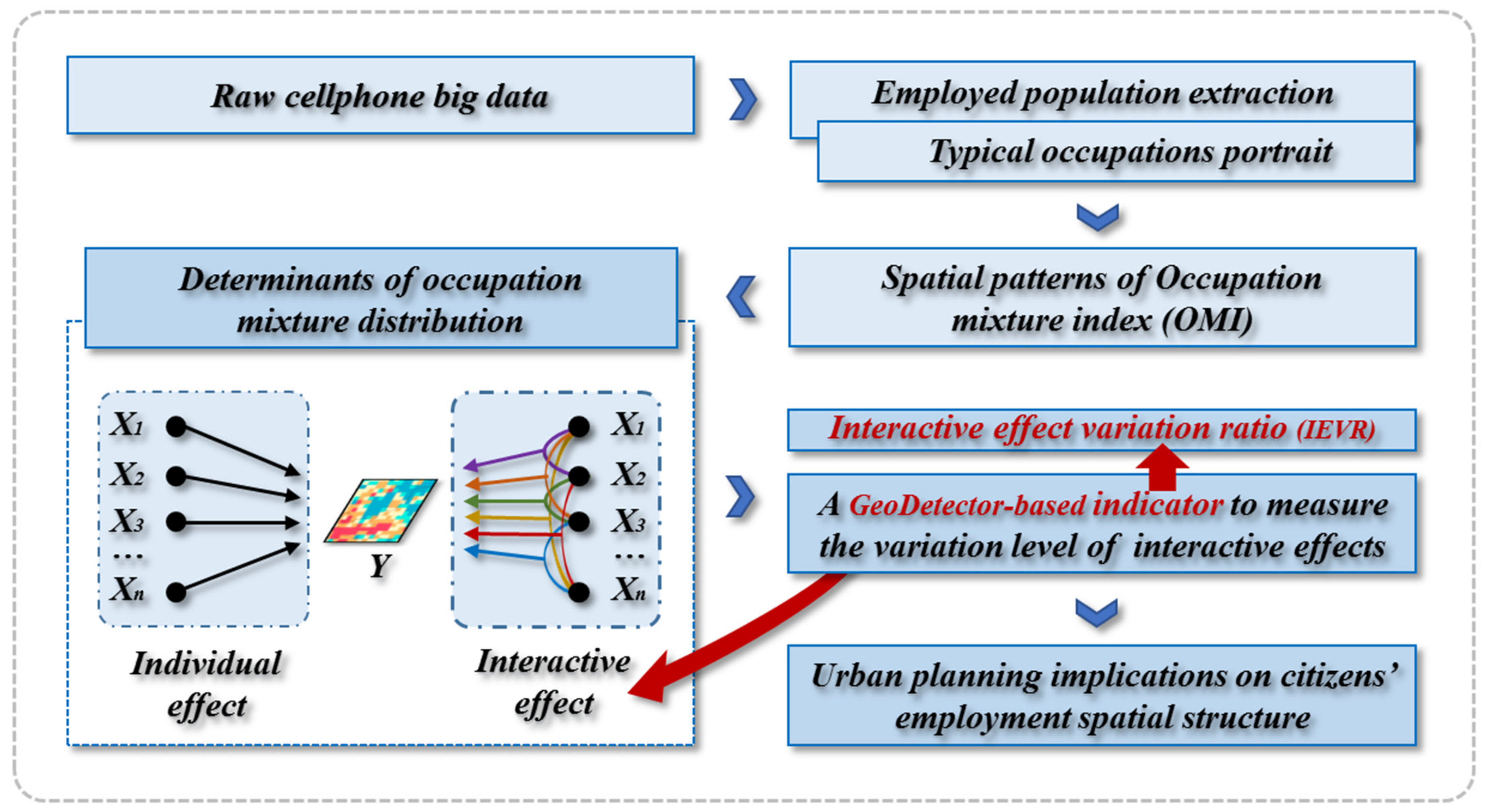
2.5. Interactive Effect Variation Ratio (IEVR)

Previous studies have proved that the combination of factor detector and interactive detector model can effectively explore the individual and interactive effects of driving factors on dependent variable [49,50,51,52]. However, how different are the individual and interactive effects of factors still remains puzzle, which also needs to be measured in a quantitative way. On the one hand, the individual effect (PD) of an independent variable can be regarded as the direct influence on the dependent variable, which is similar as the coefficient of a regression model. On the premise of passing the significance test, the higher the PD of an independent variable, the greater impact on dependent variable distribution is. On the other hand, the interactive effect of a pair of independent variables can be regarded as indirect effect correspondingly, which refers the combined effect of two independent variables on dependent variable when they interact with each other. The influence mechanism of the spatial distribution of a geographical phenomenon is comprehensive and complex, so it is not enough to rely on the individual effect analysis of each factor, and the interaction analysis among factors is a necessary supplement. On this basis, it is necessary to further quantify the differences between the interaction and individual effects of factors, and then it is possible to explore the direct and indirect influence of each factor on the dependent variable.

Therefore, a GeoDetector-based indicator, interactive effect variation ratio (IEVR) was proposed in this study to quantify the variation between individual effect (direct impact) and interactive effect (indirect impact) of potential driving factors, which is calculated as Equation (6).

$$IEV{R}_{x_i}=\frac{{\sum }_{j=1,j\ne i}^{n}PD\left(x_i\cap x_j\right)100\%}{\left(n-1\right)PD\left(x_i\right)}-1$$

(6)

where $IEV{R}_{x_i}$ represents the indirect effect on dependent variable of a independent variable ($x_i$). In other words, the average variation ratio of the interactive effects with other independent variables compared with its individual effect. n represents the number of independent variables, and n ≥ 2 generally.

The brief calculation steps of the IEVR are as follows. First, the individual effect (PD ($x_i$)) of $x_i$, and the interactive effects of each factor pair of $x_i$ with others were calculated by factor detector model and interactive detector model. Second, each difference between each factor pair of $x_i$ with others (PD ($x_i\cap x_j$)) and PD ($x_i$) is measured. Then, the average of all differences between PD ($x_i$) and PD ($x_i\cap x_j$) was calculated, which is the result of $IEV{R}_{x_i}$.

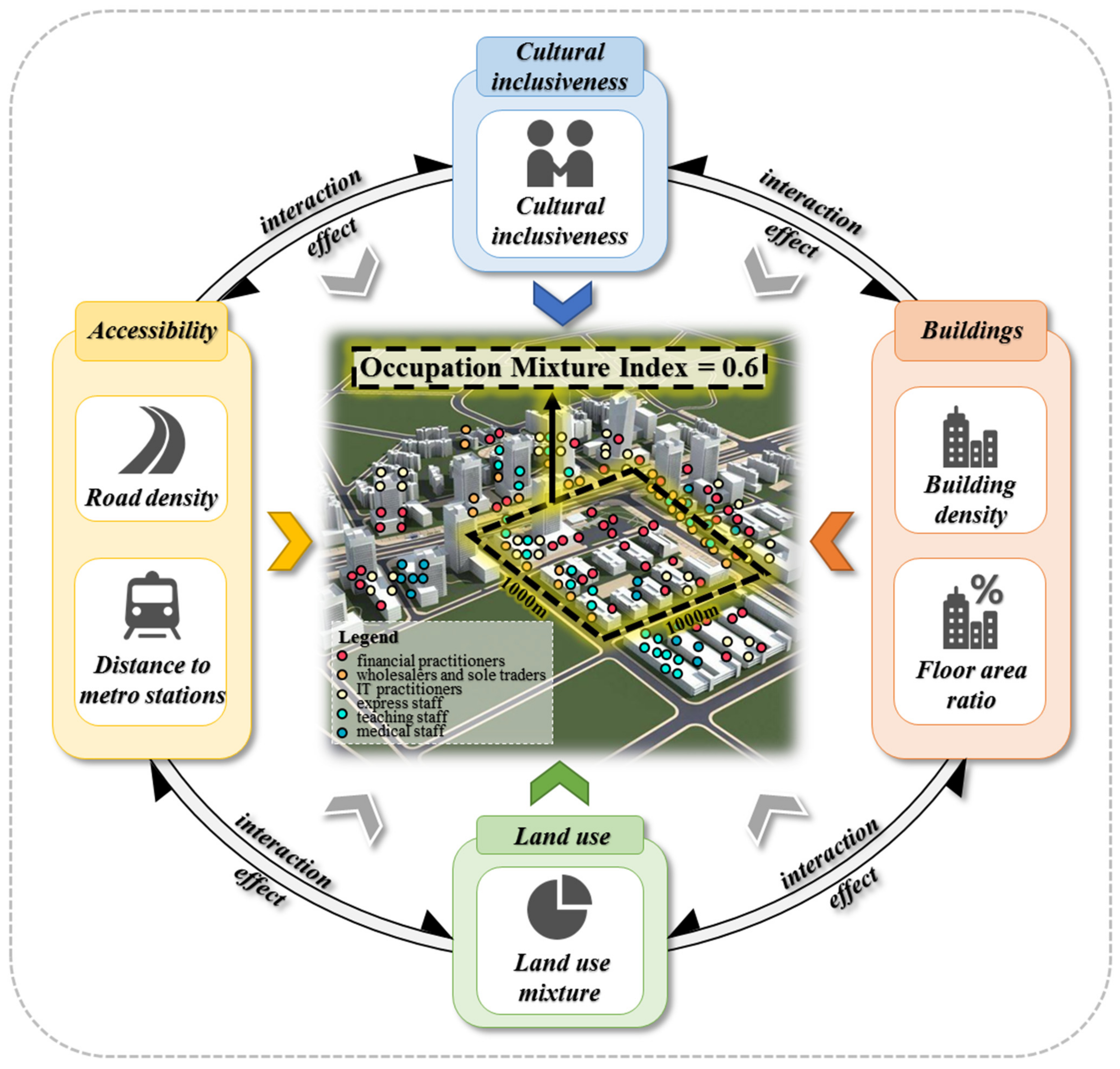
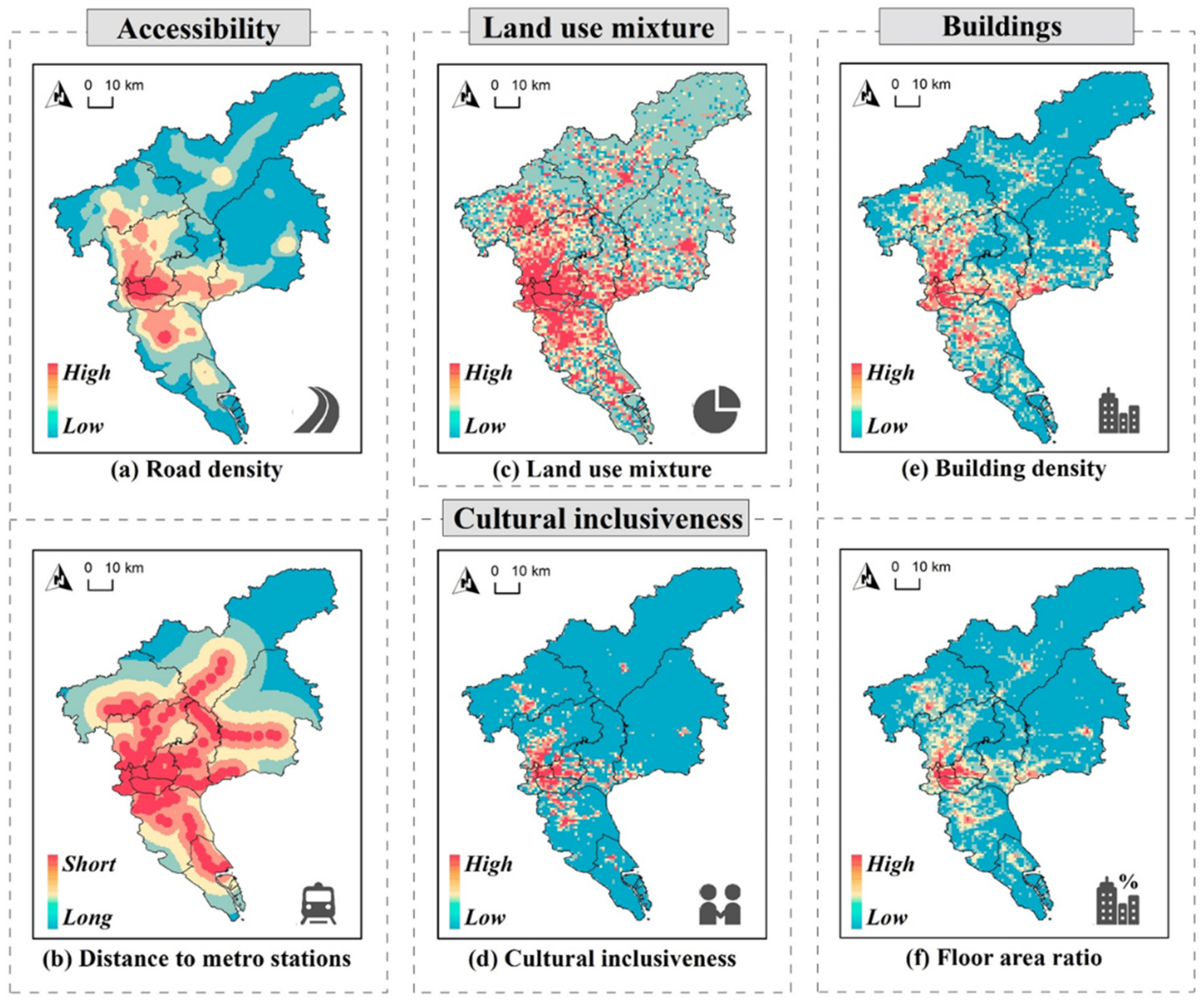
2.6. Variable Selection

It should be noticed that the mechanism of OMI is comprehensive including not only individual influence of each factor, but also the interactive effects between factors (Figure 4). Based on the literature [37,38,39,40,41] and the situation of Guangzhou, six types of potential driving factors were selected to represent the built environment from multi-perspectives including accessibility, buildings, cultural inclusiveness, and land use.

First, Road density (Road) [37] and distance to metro stations (Metro) were calculated in ArcMap 10.2 to represent accessibility. Road data were obtained from OpenStreetMap (https://www.openstreetmap.org/) in November 2020. Metro stations POIs data were collected from Baidu Map API (http://lbsyun.baidu.com/) in November 2020. Metro of each grid was calculated via the tool of Euclidean distance in ArcMap 10.7 software. Road of each grid was calculated as Equation (7).

$$Roa{d}_i=\frac{Lengt{h}_i}{Grid Are{a}_i}$$

(7)

where $Roa{d}_i$ refers to the road density of grid i; $Lengt{h}_i$ represents the roads length within grid i; $Grid Are{a}_i$ refers to the area of grid i.

Second, building density (BD) and floor area ratio (FAR) were measured in ArcMap 10.2 to represent buildings attribute from 2D and 3D perspective. Building footprint and floors data were provided by Guangzhou Urban Planning and Design Survey Research Institute. BD of each grid was calculated as Equation (8).

$$B{D}_i=\frac{Footprint Are{a}_i}{Grid are{a}_i}$$

(8)

where $B{D}_i$ refers to the building density of grid i; $Footprint Are{a}_i$represents the buildings footprint area within grid i; $Grid Are{a}_i$ refers to the area of grid i.

FAR of each grid was calculated as Equation (9).

$$FA{R}_i=\frac{Footprint Are{a}_{i,j}\times Floo{r}_{i,j}}{Grid are{a}_i}$$

(9)

where $FA{R}_i$ refers to the floor area ratio of grid i; $Footprint Are{a}_{i,j}$represents the buildings footprint area within grid i; $Floo{r}_{i,j}$ refers to the floor of the building j within grid i; $Grid Are{a}_i$ refers to the area of grid i.

Thirdly, land use mixture (Land) was used to represent the active level of local socioeconomic development, based on the Shannon entropy with POIs (obtained from Baidu Map API) [37]. The POIs were categorized into 12 groups: (1) restaurants, (2) hotels, (3) shops and retails, (4) medical facilities, (5) schools and universities, (6) companies, (7) recreational facilities, (8) public service facilities, (9) public transportation facilities, (10) residential quarters and dormitories, which is calculated as Equation (10).

$$H=-{\sum }_{i=1}^N{p}_i{\log }_n{p}_i$$

(10)

where H refers to the value of land use mixture; $p_i$ represents the percentage of the $i^{th}$ type of POIs; n represents the number of types [38].

Fourthly and noteworthy, cultural inclusiveness (CI) was selected as an aspect of built environment to analyze the association with OMI. In essence, OMI is an issue and topic of human geography, which hints that discovering the impact mechanism of OMI should be performed from the human-oriented perspective. Cultural inclusiveness is multidimensional, which can be regarded as diversity and compatibility of race, religion, nationality, registered residence, lifestyle and so on. It is assumed that in general, a city with higher cultural inclusiveness might be more friendly and harmonious to locals and those new-residents from different background. As a slogan for Guangzhou’s image goes, “Eating in Guangzhou”, food culture is an important and unique part of Guangzhou culture. Food culture originated from different regions has its own characteristics. In the process of the development of various cuisine catering industry, the stable food culture space has gradually formed.

Given the data availability and unique regional cultural characteristics of the study area, the cultural inclusiveness index (CII) was proposed in this study based on Shannon entropy with restaurants POIs. To represent the cultural inclusiveness of Guangzhou from the perspective of food culture, both cuisines all over China and foreign cuisines were considered in measuring the cultural inclusiveness index. The applied restaurants POIs were classified into 21 types including (1) Muslim food, and foreign restaurants: (2) German cuisine, (3) French cuisine, (4) Korean cuisine, (5) Japanese cuisine, (6) Thai and Vietnamese cuisine, (7) Italy cuisine, (8) Indian cuisine, and Chinese cuisine including (9) Taiwan cuisine, (10) Beijing cuisine, (11) Chaozhou cuisine, (12) Dongbei cuisine, (13) Fujian cuisine, (14) Cantonese cuisine, (15) Hubei cuisine, (16) Hunan cuisine, (17) Shandong cuisine, (18) Shanghai cuisine, (19) Sichuan cuisine, (20) Anhui cuisine, (21) Xibei cuisine, which is calculated as Equation (11).

$$Culturalinclusivenessindex(CII)=-{\sum }_{i=1}^N{p}_i{\log }_n{p}_i$$

(11)

where $p_i$ represents the percentage of the $i\mathrm{th}$ type of cuisine POIs; n represents the number of cuisines.

All calculations of the potential driving factors were performed with ArcMap 10.2. It should be noticed that the modifiable areal unit problems (MAUP), scale effect and zoning effect, might affect the GeoDetector model results significantly. In this study, scale effect can be excluded since that the spatial scale of the dependent variable was fixed (OMI from 1 km-grid-aggregated cellphone data), and thus the independent variables were aggregated with the same 1 km grid correspondingly. Finally, this study followed the GeoDetector MAUP test framework by Gao et al. [21] to select the suitable zoning method. This study classified the variables into 5 categories from 1 to 5 with natural breaks method after comparative tests with several zoning methods including natural breaks, equal interval and quantile method.

Finally, the spatial distribution of six processed factors were shown as Figure 5.

3. Results and Discussion

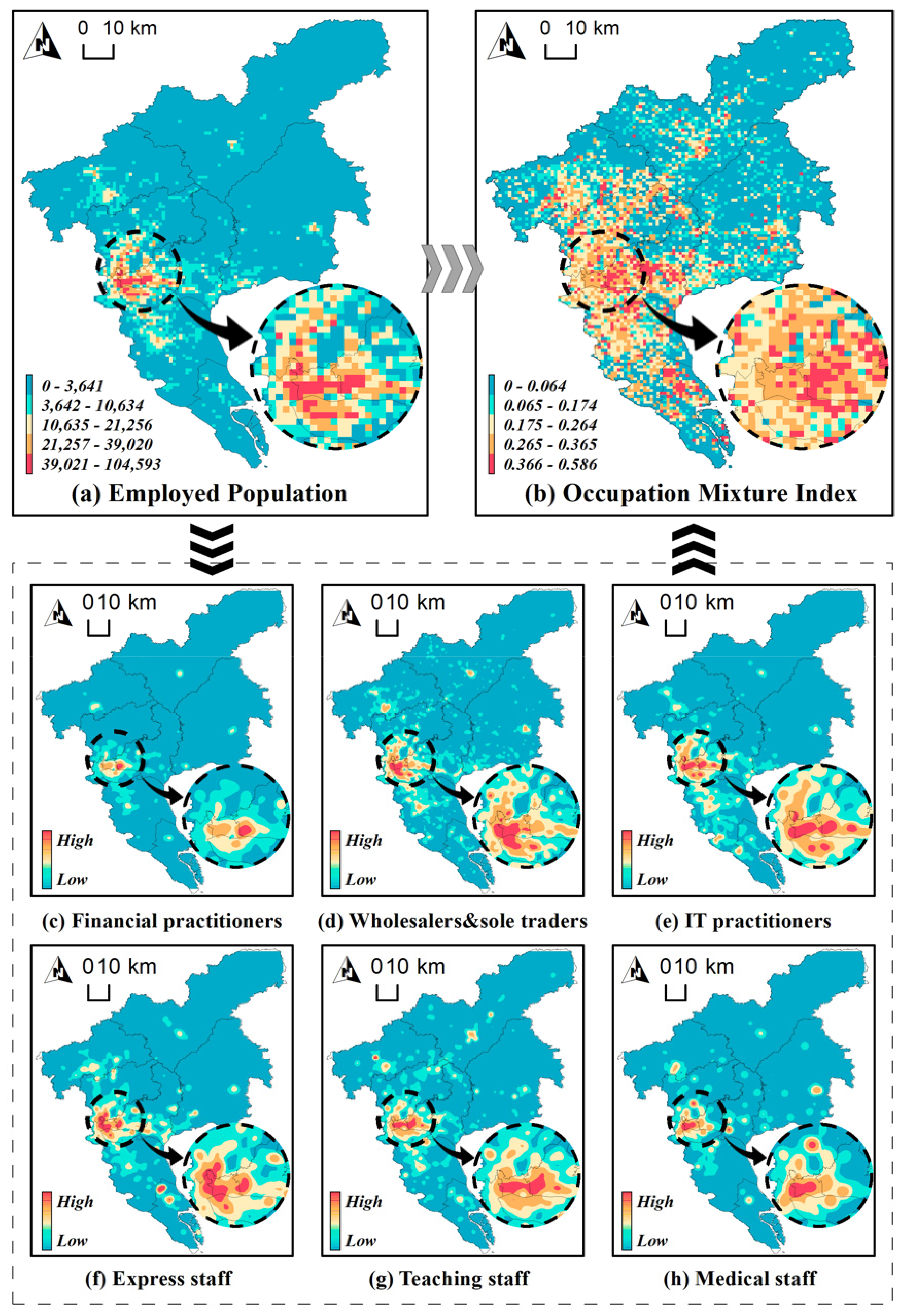
3.1. Spatial Distribution of Occupation Mixture Index

Firstly, the spatial distribution of employed population or workplace were identified as Figure 6a. The spatial distribution shows the characteristics of single core center, which is the downtown area of Guangzhou (highlighted with circle). Most employed population were located in Yuexiu district, western Tianhe district, eastern Liwan district, western Haizhu district. In terms of suburbs, locally and relatively high dense of employed population were observed at the local town centers or along the major roads, but much lower than downtown area. A linear correlation was applied in validating the result of employed population identification in this study with corresponding population census data in 2020. The employed population identification was tested to be significantly correlated with census data with the correlation coefficient of 0.84.

Secondly, based on the framework by Zhang et al. [10], six types of common occupations of employed population were portrayed and the spatial patterns of them were shown as Figure 6c–h: financial practitioners (Figure 6c), wholesalers and sole traders (Figure 6d), IT practitioners (Figure 6e), express staff (Figure 6f), teaching staff (Figure 6g), medical staff (Figure 6h). As shown in Figure 6, the spatial heterogeneity of each occupations’ practitioner density was different. The density distributions of financial practitioners, teaching staff and medical staff tended to be more compact and focused on the Yuexiu and Tianhe districts. While the densities of wholesalers and sole traders, IT practitioners and express staff were polycentric distribution.

Thirdly, after portraying six types of occupation practitioners, the occupation mixture of Guangzhou was measured and its spatial distribution is shown in Figure 6b. To make the visualizations of Figure 6a,b clear and easy for comparison, the natural breaks method was applied for color grading of two images. The distribution patterns of employed population and occupation mixture index were significantly different that the former was highly concentrated in downtown, while the latter was much more uniform with high value of OMI covering both downtown area and suburbs. It was noticed that Yuexiu district was the center of employment quantity, and that the center of employment diversity was located in Tianhe district.

Figure 6a reflected the employed population density of the city, and Figure 6b further answered how diverse were the workplaces in Guangzhou. In the next section, this study investigated the influence of potential driving factors on the spatial distribution of OMI.

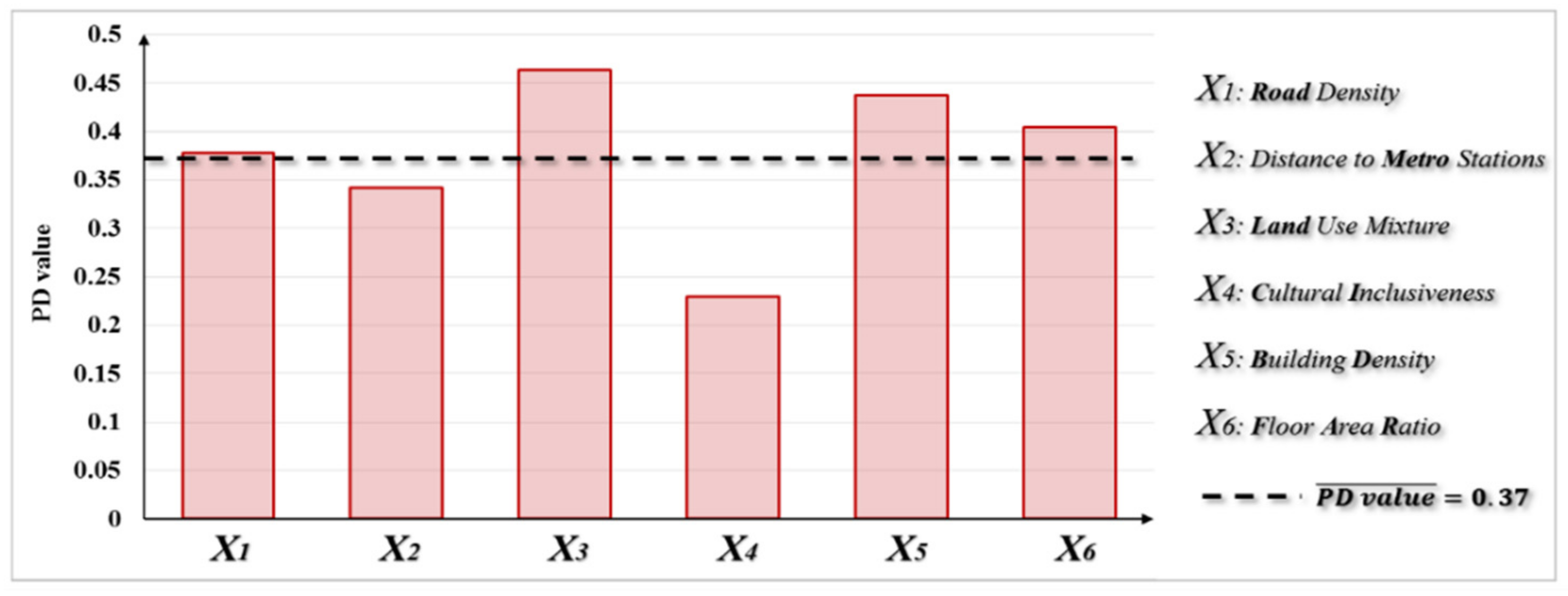
3.2. Individual Effects of Determinants on OMI

The factor detector, sub-model of GeoDetector model was applied to examine the individual effect of six selected potential driving factors on OMI distribution. The results showed that all selected variables significantly contributed to the OMI distribution with p-values lower than 0.01 (Figure 7). Land was found to be the most influential variable with the strongest individual impact on OMI, followed by BD, FAR, Road, Metro and CI. Among all the variables, the effects of Land, BD, FAR and Road were higher than average level (0.37). It indicated that the influences of these factors on OMI were in a relatively direct way.

In regard of land use mixture, the most influential variable, it represents the active level of local socioeconomic development. Its PD value reached 0.45, that is, land use mixture explained over 45% of the spatial distribution of OMI according to the theory of GeoDetector model. Both Land and the dependent variable, OMI, were indices assessing diversity level with Shannon entropy. Land use mixture represents the diversity of various types of urban service facilities. Its highest impact on OMI among four considered aspects of variables indicated that satisfactory hardware facilities was the solid foundation for urban development and residents’ life. Higher level of land use diversity provides conditions for life, work and transportation, contributes to the economic prosperity and development, and hence it is capable to embrace various socioeconomic activities and people from all walks of life. It hinted that the promoting in land use mixture can effectively enhance the level of occupation mixture index distribution.

In regard of buildings, its influence was also at high level, following the land use. Results showed that the 2D measurement of buildings (BD) was more influential than 3D measurement (FAR) on OMI. In terms of the impact of OMI, buildings provided employment space for all types of industries. Therefore, the spatial distribution of BD and FAR was also closely correlated with OMI.

In regard of traffic accessibility, the effect of Road on OMI was stronger than Metro. It hinted that though rail transit was essential to a city, the spatial distribution of OMI relied more on the fundamental accessibility condition, roads network. Thus, optimizing and densifying the roads network might be efficient and helpful in promoting occupation mixture, rather than rail transit.

In regard of CI, the result of factor detector model shown that its influence on OMI ranked the last among all the variables, which indicated that CI can only explained less than 25% of the OMI distribution. Specifically, the PD values of CI and Metro were lower than the average. In other words, the individual influences of these two variables on the spatial distribution of OMI were very limited, compared with other variables with above average PD values.

Numerous studies in potential influencing factors on dependent variable solely focus on each variable’s individual impact with various linear regression models. However, the influence mechanism of the spatial distribution of a certain geographical phenomenon is complex. This section discussed the results of individual effects of determinants on OMI. The interactive effects of determinants were introduced are in the next section.

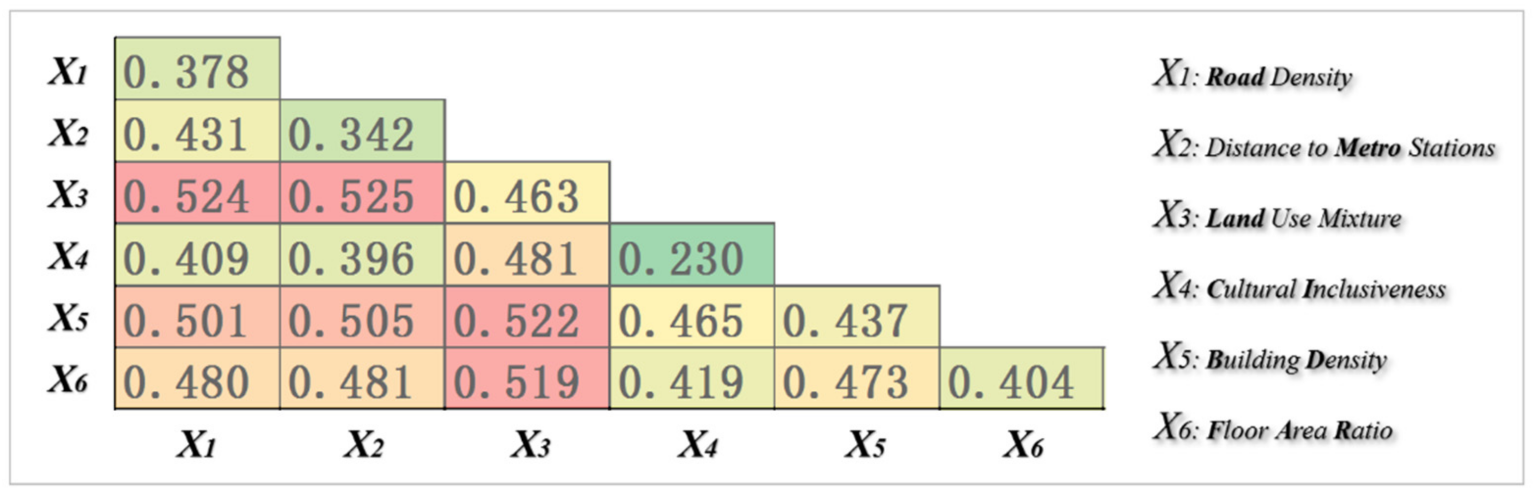
3.3. Interactive Effects of Determinants on OMI

The results of the interactive effects on OMI were shown as Figure 8. First, the interactive effects of 15 pairs of determinants were all higher than its original individual effects. Second, the interactive effect of$Land\cap Metro$ on OMI was the strongest with the interactive PD value reaching 0.525, followed by $Land\cap Road$ (0.524), $Land\cap BD$ (0.522), $Land\cap FAR$ (0.519), $BD\cap Metro$ (0.505). The above top 5 pairs of determinants proved that the Land was the crucial factor affecting the spatial distribution of OMI from the perspective of both individual and interactive effects. The interactive effect of $Land\cap Metro$ indicated that areas with high level of metro accessibility to metro stations and land use mixture tended to be with the distribution of high occupation mixture.

Moreover, it was noticed that the top two pairs of determinants were the combinations of land use mixture and traffic accessibility (Metro and Road), which suggested that the foundation of urban facilities and accessibility condition were the priorities in promoting occupation mixture. The top three and top four pairs of determinants were the interactions of land use mixture and building measurement indices (BD and FAR), which hinted that the places providing employment spaces also contributed to the spatial distribution of OMI.

Previous studies with the GeoDetector model (interactive detector sub model) solely evaluated and explained the interactive degree of factors by ranking them with interactive PD values. The difference between the individual and interactive effects of potential driving factors still remained unclear. To further quantify the differences between individual and interactive effects, a GeoDetector-based indicator, IEVR was proposed in this study. The main function of IEVR is first to distinguish whether the performance of interactive effects (PD values of interactive detector model) of a variable with others enhance or weaken compared with its individual effect (PD value of factor detector model), and then to quantify the variation ratio of interactive effects compared with individual effect. The results of IEVR of determinants were shown as Figure 9.

It was outstanding that IEVR varied greatly among determinants. First, all the IEVR were positive (>0), that is, all interactive effects were enhanced compared with individual effect, which was also mentioned in interactive effect results. Then, the ranking of factors by IEVR was significantly different from the results of individual and interactive effects. It was noticed that the CI ranked the first with an IEVR approaching 90%, followed by Metro, Road, FAR, BD, Land. In other words, the average variation (enhancement) ratio of CI’s interactive effects compared with its individual effect was near 90%. The interactive effects of CI were almost the double of its individual effect, which hinted that the role of CI in relationship with OMI tended to be indirect effect. Its individual direct impact regardless of other variables was low, while its interactive indirect effects with others were much stronger. Unlike buildings and roads, CI is a type of “soft facility” of a city, its individual direct impact on OMI was limited without other prior conditions. Only when CI interacts with other aspects of built environment can it serve as a helpful and meaningful role generating interactive effects on OMI. A satisfactory level of CI can help reducing regional discrimination and social segregation, providing sense of safety and social welfare to resident, and therefore contribute to the spatial distribution of OMI with the foundation of other built environment factors. Apart from CI, Metro also was the variable with high indirect effects interacting with other variables. CI and Metro were at the bottom of the individual effect rankings, however, the IEVR of them were way above average, which indicating that CI and Metro belonged to variables with indirectly strong effects on OMI.

4. Conclusions

This study identified six types of occupation practitioners and measured the occupation mixture distribution in Guangzhou with cellphone big data. Then, considering the data availability and the regional characteristics of the study area, six potential driving factors were selected, among which the cultural inclusiveness was put forward based on cuisines POIs data and Shannon entropy, as an aspect of built environment factors. GeoDetector model was applied to investigate the potential driving factors on the spatial distribution of OMI from the perspective of directly individual effects and indirect interactive effects. Finally, the IEVR was proposed in this study to further quantify the difference between individual effect and interactive effects of each variable. Major results were listed as follows.

• Results of GeoDetector (factor detector) model showed that Land was the factor with highest level of direct influence on OMI, and that the direct impacts of Land, BD, FAR, Road were at high level.
• Interactive detector model showed that the interactive effects were significant when land use mixture interacted with accessibility factors (Metro and Road) or building factors (BD and FAR).
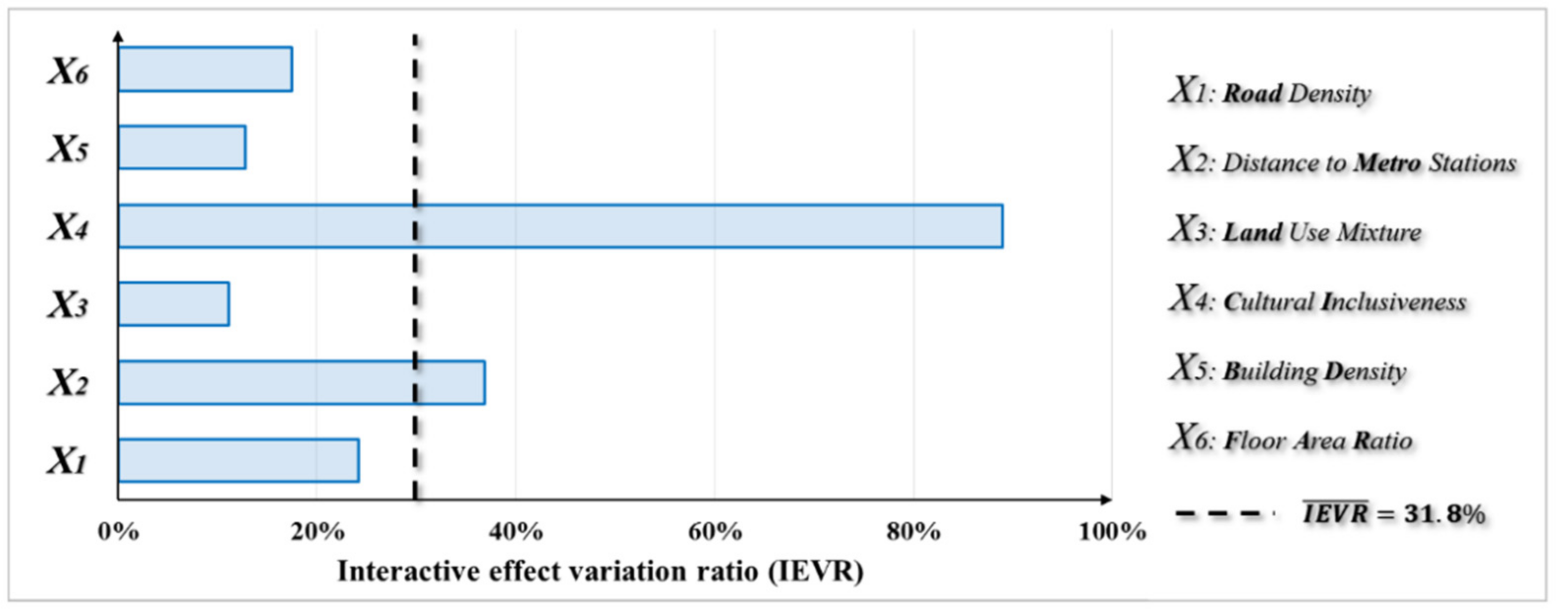
• By proposing the IEVR, some interesting results were found: CI and Metro contributed less to the distribution of OMI from factor detector and interactive detector model, while their interactive effect enhancement were at a high level, with their IEVR ranking the first and second. That is to say, the roles of CI and Metro in affecting OMI distribution tended to be indirect, generating strong interactive effects with other factors, rather than direct effect. Though CI ranked the last in direct influence ranking list, it mattered in the interaction with other built environment factors. It was a reminder that both the direct individual effects and the indirect interactive effects of potential driving factors mattered, and that how different are the interactive effects from individual effect of each variable should be clarified in a quantitative way (IEVR).
• It should be noticed that the results of this study might shed light on urban planning and management. First, OMI was applied to evaluate the diversity of residents from the perspective of occupations in Guangzhou. Areas with high OMI were located in and around downtown, where is close to saturation relatively in land development and talent employment. Therefore, attention and planning policy should be paid to those low OMI areas (suburbs) with greater potential in the process of urban renewal and suburban development. First of all, the demands of “hardware facilities” should be met in local planning including land use mixture, building density and road density, which were found important and effective in promoting OMI. Second, the result of IEVR reminded planners that based on the solid “hardware facilities” foundation, cultural inclusiveness has great potential in increasing OMI when it interacts with other built environment factors. However, we have to realize that the function of CI is to measure the current status of cultural inclusiveness of the city, which was represented by cuisine POIs. That is, CI was a variable substituting the realistic cultural inclusiveness, which was irreversible. Therefore, densifying the restaurants of different cuisines might not help improving CI and OMI. To achieve it, reforming the household registration and talent introduction policy might be helpful to build a harmonious and friendly pluralistic society.

The contributions of this study can be summarized as follows. Firstly, the results of the study outreached other similar studies in two ways. On the one hand, previous studies have been devoted into analyzing the mechanism of spatio-temporal dynamic of population distribution [37,38,39,40,41], and this study extended the understanding of population distribution by taking the internal diversity of population (OMI) into consideration. On the other hand, the individual influences of driving factors were examined in related cases using regression models [37,38], whereas the interactive effect and the variation between individual and interactive effect were seldom applied. This study explored both individual and interactive effects of variables on OMI, and their differences were also quantified. Secondly, in terms of methodology, IEVR was proposed based on the traditional GeoDetector model with the function of quantifying the difference between the individual and interactive effect of driving factors on dependent variable, then inferring whether the effect of each factor is direct or indirect. The IEVR proposed in this study provided a novel quantitatively way to explore the geographical mechanism study.

Despite the merits, limitations remaining unsolved should be noticed in future study. Similar with other cases, results extracted from cellphone big data faced difficulties in validations. Due to the data anonymity, the reliability of the occupations identification was not directly examined, which should be validated with other data sources in the future. Future work should be extended by obtaining more information from cellphone data, such as the income level and daily commuting behavior of different occupations. Additionally, the mechanism of OMI should be further explored considering both spatial and temporal dynamic using geographically and temporally weighted regression model. Moreover, OMI might be simulated with other data sources and methods including agent-based model and cellular automata model.

References

- Wu, R.; Li, Z.; Wang, S. The varying driving forces of urban land expansion in China: Insights from a spatial-temporal analysis. Sci. Total Environ. 2020, 766, 142591. [Google Scholar] [CrossRef]
- Xu, G.; Jiao, L.M.; Liu, J.F.; Shi, Z.K.; Zeng, C.; Liu, Y.L. Understanding urban expansion combining macro patterns and micro dynamics in three southeast Asian megacities. Sci. Total Environ. 2019, 660, 375–383. [Google Scholar] [CrossRef]
- Yang, Z.W.; Chen, Y.B.; Guo, G.H.; Zheng, Z.H.; Wu, Z.F. Using nighttime light data to identify the structure of polycentric cities and evaluate urban centers. Sci. Total Environ. 2021, 780, 146586. [Google Scholar] [CrossRef]
- Li, J.G.; Li, J.W.; Yuan, Y.Z.; Li, G.F. Spatiotemporal distribution characteristics and mechanism analysis of urban population density: A case of Xi’an, Shaanxi, China. Cities 2019, 86, 62–70. [Google Scholar] [CrossRef]
- Deng, C.B.; Wu, C.S.; Wang, L. Improving the housing-unit method for small-area population estimation using remote-sensing and GIS information. Int. J. Remote Sens. 2010, 31, 5673–5688. [Google Scholar] [CrossRef]
- De Montjoye, Y.A.; Hidalgo, C.A.; Verleysen, M.; Blondel, V.D. Unique in the crowd: The privacy bounds of human mobility. Sci. Rep. 2013, 3, 1376. [Google Scholar] [CrossRef] [Green Version]
- Murray, A.T.; Davis, R.; Stimson, R.J.; Ferreira, L. Public transportation access. Transp. Res. Part D Transp. Environ. 1998, 3, 319–328. [Google Scholar] [CrossRef] [Green Version]
- Pattnaik, S.B.; Mohan, S.; Tom, V.M. Urban bus transit route network design using genetic algorithm. J. Transp. Eng. 1998, 124, 368–375. [Google Scholar] [CrossRef]
- Chen, Y.M.; Liu, X.P.; Li, X.; Liu, X.J.; Yao, Y.; Hu, G.H.; Xu, X.C.; Pei, F.S. Delineating urban functional areas with building-level social media data: A dynamic time warping (DTW) distance based k-medoids method. Landsc. Urban Plan 2016, 160, 48–60. [Google Scholar] [CrossRef]
- Zhang, X.; Gao, F.; Liao, S.; Zhou, F.; Cai, G.; Li, S. Portraying Citizens’ Occupations and Assessing Urban Occupation Mixture with Mobile Phone Data: A Novel Spatiotemporal Analytical Framework. ISPRS Int. J. Geo-Inf. 2021, 10, 392. [Google Scholar] [CrossRef]
- Zhou, X.; Yeh, A.; Li, W.; Yue, Y. A commuting spectrum analysis of the jobs–housing balance and self-containment of employment with mobile phone location big data. Environ. Plan. B 2018, 45, 434–451. [Google Scholar] [CrossRef]
- Zhou, X.; Yeh, A.G.O. Understanding the modifiable areal unit problem and identifying appropriate spatial unit in jobs–housing balance and employment self-containment using big data. Transportation 2020, 48, 1267–1283. [Google Scholar] [CrossRef]
- Zhou, X.; Yeh, A.G.O.; Yue, Y. Spatial variation of self-containment and jobs-housing balance in Shenzhen using cellphone big data. J. Transp. Geogr. 2018, 68, 102–108. [Google Scholar] [CrossRef]
- Tang, J.J.; Liu, F.; Wang, Y.H.; Wang, H. Uncovering urban human mobility from large scale taxi GPS data. Phys. A Stat. Mech. Appl. 2015, 438, 140–153. [Google Scholar] [CrossRef]
- Brown, A.; LaValle, W. Hailing a change: Comparing taxi and ridehail service quality in Los Angeles. Transportation 2021, 48, 1007–1031. [Google Scholar] [CrossRef]
- Yang, H.; Liang, Y.; Yang, L. Equitable? Exploring ridesourcing waiting time and its determinants. Transp. Res. Part D Transp. Environ. 2021, 93, 102774. [Google Scholar] [CrossRef]
- Zhong, C.; Manley, E.; Arisona, S.M.; Batty, M.; Schmitt, G. Measuring variability of mobility patterns from multiday smart-card data. J. Comput. Sci. 2015, 9, 125–130. [Google Scholar] [CrossRef]
- Li, S.; Lyu, D.; Liu, X.; Tan, Z.; Gao, F.; Huang, G.; Wu, Z. The varying patterns of rail transit ridership and their relationships with fine-scale built environment factors: Big data analytics from Guangzhou. Cities 2020, 99, 102580. [Google Scholar] [CrossRef]
- Li, S.; Lyu, D.; Huang, G.; Zhang, X.; Gao, F.; Chen, Y.; Liu, X. Spatially varying impacts of built environment factors on rail transit ridership at station level: A case study in Guangzhou, China. J. Transp. Geogr. 2020, 82, 102631. [Google Scholar] [CrossRef]
- Shen, Y.; Zhang, X.; Zhao, J. Understanding the usages of dockless bike sharing in Singapore. Int. J. Sustain. Transp. 2018, 12, 686–700. [Google Scholar] [CrossRef]
- Gao, F.; Li, S.; Tan, Z.; Wu, Z.; Zhang, X.; Huang, G.; Huang, Z. Understanding the modifiable areal unit problem in dockless bike sharing usage and exploring the interactive effects of built environment factors. Int. J. Geogr. Inf. Sci. 2021, 35, 1–21. [Google Scholar] [CrossRef]
- Gao, F.; Li, S.; Tan, Z.; Zhang, X.; Lai, Z.; Tan, Z. How Is Urban Greenness Spatially Associated with Dockless Bike Sharing Usage on Weekdays, Weekends, and Holidays? ISPRS Int. J. Geo-Inf. 2021, 10, 238. [Google Scholar] [CrossRef]
- Cao, Z.; Gao, F.; Li, S.; Wu, Z.; Guang, W.; Ho, H. Ridership exceedance exposure risk: Novel indicators to assess PM2.5 health exposure of bike sharing riders. Environ. Res. 2021, 197, 111020. [Google Scholar] [CrossRef]
- Li, S.; Zhuang, C.; Tan, Z.; Gao, F.; Lai, Z.; Wu, Z. Inferring the trip purposes and uncovering spatio-temporal activity patterns from dockless shared bike dataset in Shenzhen, China. J. Transp. Geogr. 2021, 91, 102974. [Google Scholar] [CrossRef]
- Li, C.; Hu, J.; Dai, Z.; Fan, Z.; Wu, Z. Understanding Individual Mobility Pattern and Portrait Depiction Based on Mobile Phone Data. ISPRS Int. J. Geo-Inf. 2020, 9, 666. [Google Scholar] [CrossRef]
- Gao, S. Spatio-temporal analytics for exploring human mobility patterns and urban dynamics in the mobile age. Spat. Cogn. Comput. 2014, 15, 86–114. [Google Scholar] [CrossRef]
- Cao, Z.; Wu, Z.; Li, S.; Ma, W.; Deng, Y.; Sun, H.; Guan, W. Exploring spatiotemporal variation characteristics of exceedance air pollution risk using social media big data. Environ. Res. Lett. 2020, 15, 114049. [Google Scholar] [CrossRef]
- Cao, Z.; Wu, Z.; Li, S.; Guo, G.; Song, S.; Deng, Y.; Ma, W.; Sun, H.; Guan, W. Explicit Spatializing Heat-Exposure Risk and Local Associated Factors by coupling social media data and automatic meteorological station data. Environ. Res. 2020, 188, 109813. [Google Scholar] [CrossRef]
- Wang, B.; Meng, B.; Wang, J.; Chen, S.; Liu, J. Perceiving Residents’ Festival Activities Based on Social Media Data: A Case Study in Beijing, China. ISPRS Int. J. Geo-Inf. 2021, 10, 474. [Google Scholar] [CrossRef]
- Jiang, W.; Wang, Y.; Xiong, Z.; Song, X.; Long, Y.; Cao, W. Detecting Urban Events by Considering Long Temporal Dependency of Sentiment Strength in Geotagged Social Media Data. ISPRS Int. J. Geo-Inf. 2021, 10, 322. [Google Scholar] [CrossRef]
- Han, S.; Liu, C.; Chen, K.; Gui, D.; Du, Q. A Tourist Attraction Recommendation Model Fusing Spatial, Temporal, and Visual Embeddings for Flickr-Geotagged Photos. ISPRS Int. J. Geo-Inf. 2021, 10, 20. [Google Scholar] [CrossRef]
- Wang, Z.; Ma, D.; Pang, R.; Xie, F.; Zhang, J.; Sun, D. Research Progress and Development Trend of Social Media Big Data (SMBD): Knowledge Mapping Analysis Based on CiteSpace. ISPRS Int. J. Geo-Inf. 2020, 9, 632. [Google Scholar] [CrossRef]
- Ahas, R.; Aasa, A.; Silm, S.; Tiru, M. Daily rhythms of suburban commuters’movements in the Tallinn metropolitan area: Case study with mobile positioning data. Transp. Res. Part C Emerg. Technol. 2010, 18, 45–54. [Google Scholar] [CrossRef]
- García-Palomares, J.C.; Salas-Olmedo, M.H.; Moya-Gómez, B.; Condeço-Melhorado, A.; Gutiérrez, J. City dynamics through Twitter: Relationships between land use and spatiotemporal demographics. Cities 2018, 72, 310–319. [Google Scholar] [CrossRef]
- Liu, K.; Murayama, Y.; Ichinosec, T. Exploring the relationship between functional urban polycentricity and the regional characteristics of human mobility: A multi-view analysis in the Tokyo metropolitan area. Cities 2021, 111, 103109. [Google Scholar] [CrossRef]
- Liu, K.; Murayama, Y.; Ichinosec, T. A multi-view of the daily urban rhythms of human mobility in the Tokyo metropolitan area. J. Transp. Geogr. 2021, 91, 102985. [Google Scholar] [CrossRef]
- Wu, C.; Ye, X.; Ren, F.; Du, Q. Check-in behaviour and spatio-temporal vibrancy: An exploratory analysis in Shenzhen, China. Cities 2019, 77, 104–116. [Google Scholar] [CrossRef]
- Tu, W.; Zhu, T.; Xia, J.; Zhou, Y.; Lai, Y.; Jiang, J.; Li, Q. Portraying the spatial dynamics of urban vibrancy using multisource urban big data. Comput. Environ. Urban Syst. 2020, 80, 101428. [Google Scholar] [CrossRef]
- Guo, X.; Chen, H.; Yang, X. An Evaluation of Street Dynamic Vitality and Its Influential Factors Based on Multi-Source Big Data. ISPRS Int. J. Geo-Inf. 2021, 10, 143. [Google Scholar] [CrossRef]
- Meng, Y.; Xing, H. Exploring the relationship between landscape characteristics and urban vibrancy: A case study using morphology and review data. Cities 2019, 95, 102389. [Google Scholar] [CrossRef]
- Fu, R.; Zhang, X.; Yang, D.; Cai, T.; Zhang, Y. The Relationship between Urban Vibrancy and Built Environment: An Empirical Study from an Emerging City in an Arid Region. Int. J. Environ. Res. Public Health 2021, 18, 525. [Google Scholar] [CrossRef]
- Murphy, R.E.; Vance, J.E. Delimiting the CBD. Econ. Geogr. 1954, 30, 34. [Google Scholar] [CrossRef]
- Berry, B.J.L.; Garrisson, W.L. The functional bases of the central-place hierarchy. Econ. Geogr. 1958, 34, 145–154. [Google Scholar] [CrossRef]
- Carol, H. The hierarchy of central functions within the city. Ann. Assoc. Am. Geogr. 1960, 50, 419–438. [Google Scholar] [CrossRef]
- Preston, R.E. The structure of central place systems. Econ. Geogr. 1971, 47, 136–155. [Google Scholar] [CrossRef]
- Alonso, W. A Theory of The Urban Land Market. Pap. Reg. Sci. 2005, 6, 149–157. [Google Scholar] [CrossRef]
- Fotheringham, A.S.; Brunsdon, C.; Charlton, M. Geographically Weighted Regression; John Wiley & Sons, Limited: Hoboken, NJ, USA, 2003. [Google Scholar]
- Griffith, D.A. A spatial filtering specification for the autologistic model. Environ. Plan. A 2004, 36, 1791–1811. [Google Scholar] [CrossRef] [Green Version]
- Wang, J.; Li, X.; Christakos, G.; Liao, Y.; Zhang, T.; Gu, X.; Zheng, X. Geographical Detector—Based Health Risk Assessment and its Application in the Neural Tube Defects Study of the Heshun Region, China. Int. J. Geogr. Inf. Sci. 2010, 24, 107–127. [Google Scholar] [CrossRef]
- Wang, J.; Zhang, T.; Fu, B. A measure of spatial stratified heterogeneity. Ecol. Indic. 2016, 67, 250–256. [Google Scholar] [CrossRef]
- Wang, J.; Hu, Y. Environmental health risk detection with GeogDetector. Environ. Model. Softw. 2012, 33, 114–115. [Google Scholar] [CrossRef]
- Zhang, Q.; Wu, Z.; Tarolli, P. Investigating the Role of Green Infrastructure on Urban WaterLogging: Evidence from Metropolitan Coastal Cities. Remote Sens. 2021, 13, 2341. [Google Scholar] [CrossRef]
- Zheng, Z.; Zhou, S.; Deng, X. Exploring both home-based and work-based jobs-housing balance by distance decay effect. J. Transp. Geogr. 2021, 93, 103043. [Google Scholar] [CrossRef]
Publisher’s Note: MDPI stays neutral with regard to jurisdictional claims in published maps and institutional affiliations. |
© 2021 by the authors. Licensee MDPI, Basel, Switzerland. This article is an open access article distributed under the terms and conditions of the Creative Commons Attribution (CC BY) license (https://creativecommons.org/licenses/by/4.0/).
Share and Cite
Deng, X.; Liu, Y.; Gao, F.; Liao, S.; Zhou, F.; Cai, G. Spatial Distribution and Mechanism of Urban Occupation Mixture in Guangzhou: An Optimized GeoDetector-Based Index to Compare Individual and Interactive Effects. ISPRS Int. J. Geo-Inf. 2021, 10, 659. https://0-doi-org.brum.beds.ac.uk/10.3390/ijgi10100659
Deng X, Liu Y, Gao F, Liao S, Zhou F, Cai G. Spatial Distribution and Mechanism of Urban Occupation Mixture in Guangzhou: An Optimized GeoDetector-Based Index to Compare Individual and Interactive Effects. ISPRS International Journal of Geo-Information. 2021; 10(10):659. https://0-doi-org.brum.beds.ac.uk/10.3390/ijgi10100659
Chicago/Turabian StyleDeng, Xingdong, Yang Liu, Feng Gao, Shunyi Liao, Fan Zhou, and Guanfang Cai. 2021. "Spatial Distribution and Mechanism of Urban Occupation Mixture in Guangzhou: An Optimized GeoDetector-Based Index to Compare Individual and Interactive Effects" ISPRS International Journal of Geo-Information 10, no. 10: 659. https://0-doi-org.brum.beds.ac.uk/10.3390/ijgi10100659