The Land-Use Change Dynamics Based on the CORINE Data in the Period 1990–2018 in the European Archipelagos of the Macaronesia Region: Azores, Canary Islands, and Madeira

Abstract

Islands as peripheral and ultra-peripheral are typically highlighted as ecologically sensitive areas to human activities due to the tremendous biological diversity of beings and the future possibility of habitat loss. In this regard, the comprehension of the land occupation dynamics and trends in the ultra-peripheral territories is crucial to attempt long-lasting regional sustainability, as is the island region’s case. Therefore, the present article aims to analyze the trends and dynamics of the land-use changes on the European Archipelagos of the Macaronesia Region over the last three decades, using the CORINE (Coordination of Information on the Environment) data. Some of the obtained results show that about 3.4% of the Azores’ surface is characterized mainly by discontinuous urban fabric, representing 67% of the total urban fabric of the Azores over the last thirty years. Additionally, in Madeira Archipelago, the land is mainly occupied by forest and semi-natural areas, representing almost three-thirds of the territory. A similar scenario is verified in the Canary Islands, where forests and semi-natural areas represent approximately three-quarters of the territory. Once more, this study shows the relevance of the island areas’ unique character, which should be preserved and protected. Therefore, the priorities must be defined and established management strategies that are significant for the well-being of these highly valued areas. Moreover, the study showed that notable changes had occurred in the period 1990–2018 in this landscape. Hence there is a need for appropriate measures to mitigate these negative impacts on the environment.

1. Introduction

Nowadays, our societies face several challenges. Among these obstacles and requirements, we have regional planning, which is an essential requirement for the so-desired sustainable development [1,2,3,4,5,6,7,8,9]. In fact, such challenges are even more evident in ultra-peripheral territories [10,11,12,13]. Accordingly, the comprehension of the land occupation dynamics and trends in the ultraperipheral territories is crucial to attempt long-lasting regional sustainability, as is the island region’s case.

In this regard, the European Archipelagos of the Macaronesia Region (the Azores, Canary Islands, and Madeira) were selected as case studies. Consequently, the land-use changes over the last three decades were analyzed. The Azores and Madeira belong to Portugal, whereas the Canaries belong to Spain.

Changes in land-use can be associated with economic growth and investors’ search for profitable locations for the implementation of their projects, supported by local authorities to improve the economic status of local self-government [4]. This is especially harmful to areas of high environmental quality. Exceptionally high ecological values characterize these islands, so it is necessary and vital to explore the fragmentation of the landscape as monitoring the increase of anthropic pressure, especially in the vicinity of highly urbanized areas.

Fragmentation in landscape patterns can compromise its functional integrity by disrupting critical ecological processes to maintain biodiversity and ecosystem health [14]. Many anthropogenic activities (e.g., development, logging) can disrupt the structural integrity of the landscape and can sometimes facilitate ecological flows (e.g., animal movement) across the landscape [15]. Space fragmentation is a phenomenon studied by the scientific community, particularly environmentalists and urban planners (see [16,17,18,19]). There are numerous works available that refer to the problem of landscape fragmentation [20,21,22]. With increased awareness of environmental sustainability issues and intensifying land development, the importance of the CORINE database and assessment of LULC changes (Land-Use Land Change) are examined [23,24,25].

The Macaronesian region has long been overlooked in comparative LULC research for two reasons. First, compared to other mainland regions more prevalent in academic literature, the small size, and population of the islands denote spatial dynamics of lower magnitude, which may diminish interest in their study. Second, there is a chronic shortage of comparable and uniform geospatial data for this region. Temme and Verburg [26] recognize a “(...) lack of homogeneous modeling, monitoring, and mapping strategies throughout the EU”.

Up-to-date advances in geographic information technologies (GIS), where applicable FRAGSTATS as a spatial sample analysis program for categorical maps, can present the landscape through a mosaic model of landscape structure. Such a designated landscape is user-defined and can reproduce any spatial phenomenon. FRAGSTATS quantifies spatial heterogeneity and gives the user the ability to form the basis for defining and scaling landscapes in thematic content and resolution.

Contextually, this investigation is based on research techniques. These techniques and methods allow us to identify the dynamics of land-use changes in these territories. The chosen approach relies on proposing new geographical representations and modeling methods that emphasize the importance of geographical visualization of landscape fragmentation for spatial planning in this environmentally critical area. The research provides a greater understanding of the actors and decision-makers involved in how these ultra-peripheral territories have developed and how new territorial plans should be designed.

This work provides novel techniques in evaluating and managing the landscape of the study areas while considering that they could be applied in other research. Besides, the research results can contribute to the sustainable development of the islands.

Therefore, this paper begins with this initial chapter, followed by a brief overview of the literature related to the protection of ecosystem services: a Geographic Information Systems (GIS) and methodology based on CORINE land cover classes (CLC) and FRAG STATS, a methodological framework regarding the techniques used in the empirical part of the research, followed by the results, as well as their subsequent discussion and conclusions, with the final section on the limitations of the study and future research lines.

2. CORINE Land Cover and Landscape Fragmentation Analysis

The CLC database is a tool for performing complex spatial analyses based on diverse land-use kinds. CORINE land cover classes (CLC) have three levels in their hierarchical organization. The first covers five main types of land-use and land cover: artificial areas, agricultural areas, forest and semi-natural areas, wetlands, and water bodies. The next level has 15 departments. The third level includes 44 departments that note that the methodological scope of the three individual-level three classes is strictly defined [27,28,29].

The CLC records changes in land cover that are happening gradually and is very useful for research needed at the regional level. The main number of new researches has conducted territorial studies based on GIS Tools and CORINE data methodical approaches to landscape fragmentation. Especially in environmental studies as well as on research about changes in land degradation—i.e., in areas with different types of land cover countries, regions, islands, or cities [30,31,32,33], including urban growth monitoring and urban sprawl comparations’ land-use forecasts, modeling of road travel speeds or fragmentation of property rights [34].

Islands as peripheral and ultra-peripheral are usually highlighted as ecologically sensitive areas to human activities due to the tremendous biological diversity of beings and the future probability of habitat loss [35]. Many researchers also analyzed the application of land reclamation, as an intensive change of land-use can often cause devastating impacts on the processes of the existing ecosystem and subsequently affect the surrounding environment [36].

CLC is the unique LULC database covering the Macaronesian islands of Portugal and Spain. CLC data sets were used as primary data sources in the study. CLCs are a map of the European landscape based on remote sensing. These public domain data sets provide a list of land cover classes organized hierarchically in three levels as a comparable cartographic product (minimum mapping unit 25 ha). CLC level 1 corresponds to the main categories (i.e., artificial areas, agricultural areas, forests and semi-natural areas, wetlands, water bodies). CLC level 2 covers whole areas with a higher level of detail (15 classes). Finally, level 3 CLC consists of 44 land cover classes (

Table 1. Evolution of CORINE Land Cover. (Source: [27]).

	CLC1990	CLC2000	CLC2006	CLC2012	CLC2018
Satellite data	Landsat-5 MSS/TM	Landsat-7 ETM	SPOT-4/5 and	IRS P6 LISS III	Sentinel-2 and Landsat-8 for gap filling
	single date	single date	IRS P6 LISS III	and RapidEye
			dual date	dual date
Time consistency	1986–1998	2000+/−1 year	2006+/−1 year	2011–2012	2017–2018
Geometric accuracy, satellite data	≤50 m	≤25 m	≤25 m	≤25 m	≤10 m (Sentinel-2)
Min. mapping unit/width	25 ha/100 m	25 ha/100 m	25 ha/100 m	25 ha/100 m	25 ha/100 m
Geometric accuracy, CLC	100 m	better than 100 m	better than 100 m	better than 100 m	better than 100 m
Thematic accuracy, CLC	≥85% (probably not achieved)	≥85%	≥85%	≥85%	≥85%
		(achieved) [13]		(probably achieved)
Change mapping (CHA)	not implemented	boundary displacement min. 100 m	boundary displacement min. 100 m	boundary displacement min. 100 m	boundary displacement min. 100 m
		change area for existing polygons ≥5 ha; for isolated changes ≥25 ha	all changes ≥5 ha are to be mapped	all changes ≥5 ha are to be mapped	all changes ≥5 ha are to be mapped
Thematic accuracy, CHA	–	not checked	≥85%	≥85%	≥85%
			(achieved)
Production time	10 years	4 years	3 years	2 years	1.5 years
Documentation	incomplete metadata	standard metadata	standard metadata	standard metadata	standard metadata
Access to the data (CLC, CHA)	unclear dissemination policy	dissemination policy agreed from the start	free access for all users	free access for all users	free access for all users
Number of countries involved	26	30	38	39	39
	(27 with late implementation)	(35 with late implementation)

). Thus, the aggregate level of CLC 1 characterizes land-use, while CLC 2 further characterizes land cover. This research uses CLC level 1 and CLC level 2—which level is used depends on the research question. Table 1 hierarchically organizes the CLC nomenclature according to three levels: CLC level 1 (land-use) and CLC level 2, and CLC level 3 (land cover).

Landscape metrics depicting different aspects of the spatial pattern were calculated at class and landscape levels using the software FRAGSTATS [37,38,39,40]. Landscape metrics are a unique feature that allows a quantitative assessment of the landscape and its level of fragmentation [19], and an understanding of landscape structure, function, and change. Landscape metrics mainly focus on three characteristics of the landscape [38,39]: (1) Structure: spatial relationships between recognizable ecosystems or elements that are present—more precisely, the distribution of energy, materials, and species concerning the sizes, shapes, numbers, species, and configurations of ecosystems; (2) Function: interactions between spatial elements, i.e., the flow of energy, materials, and species between ecosystem components; and (3) Change: change in the ‘Ecological Mosaic’ structure and function over time [40].

Landscape metrics quantify landscape patterns and interactions between patch density, several patches, total area, and extensive patch index in a landscape mosaic. In fact, those metrics allow us to see patterns and changes in interaction over time. Landscape composition can be quantified by patch number, patch density, landscape percentage, and highest patch index [38,39,40].

3. Materials and Methods

The CORINE, Coordination of Information Environment Programme, develops the CLC project, whose main objective is to obtain a European land occupation database for territorial analysis and European policy management. This geographical database, which is the first layer used in the present research, supplies land-uses in the European Union using polygon graphic features.

As for the spatial component, the reference scale is 1:100,000, the Geodesic Reference System is European Reference Terrestrial System 1989 (ETRS89), and the Mapping System is Universal Transverse Mercator (UTM). Additionally, the minimum width recorded for linear phenomena is 100 m. For polygon phenomena, the Minimum Cartographic Unit (MCU) is 25 hectares represented by a square of 5 × 5 mm or a circle with 2.8 mm. Regarding the thematic component, it offers three hierarchical levels of information.

In this regard, the development of ETRS89 is related to the global International Terrestrial Reference System and Frame (ITRS), which describes procedures for creating reference frames suitable for use with measurements on or near the Earth’s surface. Indeed, the continental drift representation in ETRS89 is balanced since continental plates’ total apparent angular momentum is about 0.

Besides, the data is in vector format, using polygons that evoke the various land-uses organized into three hierarchical levels using 44 classes, according to the European Environmental Agency (Table 1).

The second layer of information used also consists of polygonal graphical features that evoke administrative divisions at their different levels of the three archipelagoes studied: Autonomous Region of the Azores, Autonomous Region of Madeira, and the Autonomous Region of the Canary Islands.

In the Canary Islands, the information was obtained from the Download Center of the National Center for Geographical Information, belonging to the Ministry of Transport, Mobility, and Urban Agenda of Spain’s Government. Specifically, the National Topographic Base was obtained at a 1:100,000 scale [41].

As for the Portuguese archipelagos corresponding to Azores and Madeira, the information was obtained from the National Geographic Information System, obtaining the Official Administrative Charter of Portugal in 2020 [42]. The scale is also 1:100,000.

The geodesic reference systems in the archipelago are different. In the Canary Islands, the projection is UTM and zone 27 and 28, being its EPSG (European Petroleum Survey Group) codes 4082 and 4083. So, for the Azores archipelago that also uses UTM projection, the EPSG code is 5015 in zone 26. In the case of the Madeira Archipelago, the EPSG code corresponds to 5016 in zone 28.

In this regard, EuroGeographics, where the Cartographic and Cadastral Agencies of the various European countries are represented, and the Joint Research Centre of the European Commission (EC), decided in December 2000 to entrust CERCO’s No.8 working groups (Commission European des Responsible for Cartographie Officielle (French)) and EUREF (European Reference Frame) transformations with complete development of the technical details of the conventional Coordinate Reference System for Europe, to be adopted by the EC. Accordingly, recommendations to the European Commission [43] turned out to be: (1) Adopt ETRS89 as a geodetic datum and (2) Host, for statistical analysis and presentations, the ETRS89-Azimuth Equiarea coordinate system of Lambert-2001 (ETRS-LAEA) [44]. The ETRS-LAEA is based on the projection of equivalent areas in the territory. In this way, it serves as a reference for homogeneous units for all European countries. As a result, this coordinate system is used for the representation of analytical and statistical data.

In fact, this work intends to compare the area obtained from the uses of CLC in 1990, 2000, 2006, 2012, and 2018 in the archipelagoes of the Canary Islands, Azores, and Madeira. As a result, from Feature Manipulation Engine 2020.2 (FME) software developed by the company SAFE software, all layers of information were transformed to ETRS89-LAEA.

Subsequently, all layers were managed using ArcGIS 10.5 software. Initially, in the administrative divisions’ representative layers, the islands corresponding to the archipelagoes to be studied were selected. Three layers of information were obtained, one layer for each archipelago. These layers were then merged into a single layer. This was possible because all layers used the same graphical rendering features, that is, polygons. Thus, a single layer was obtained with the delimitation of the work area. Then, geoprocessing the previous layer corresponding to the islands’ administrative delimitations and the CLC layer corresponding to 1990 were related, using the clip tool. In this case, two layers are related to polygonal graphic features. Moreover, a resulting layer with polygons containing the land-use CLC in 1990 included in the various administrative divisions of the islands, including the islands and municipalities was obtained. The associated alpha-numeric information has three fundamental fields: (1) the CLC code of each polygon, (2) the island on which the CLC land-use representative polygon is located, and (3) the municipality where each registered land-use is located. However, there was no field corresponding to the surface occupied by each of the polygons representative of the CLC land-uses within each administrative division. Thus, a geometric measurement on the ETRS89-LAEA projection in hectares of each of the various polygons representing land-uses within each municipality analyzed was carried out. To this aim, a new field of information was generated, and with this, the area was geometrically calculated in hectares.

This procedure linking the islands’ administrative divisions and land-uses for 1990 was also repeated for 2000, 2006, 2012, and 2018. In this way, a table of information was obtained for each of the years analyzed. The alphanumeric information obtained for each previous year was then exported and integrated into a Microsoft Access-managed database belonging to the Microsoft Office 365 package.

Moreover, a query was made using a structured query language (SQL) to select land-uses for each of the islands in 1990. Then, the previous query was queried by CLC codes of the registered hectares, also using SQL. So, a table was obtained with the CLC land-uses and the corresponding hectares on each of the islands for 1990, 2000, 2006, 2012, and 2018. Then, to compare the area obtained on each of the islands and archipelagos, it was necessary to normalize the data. Thus, the percentage occupied by each of the land-uses classified according to the CLC code was calculated relative to the total area of the corresponding archipelago for the first and third CLC level.

The calculation of landscape fragmentation analysis was then performed. For this purpose, CLC land-uses were used for the archipelagoes studied in 1990 and 2018. First, for each of the three archipelagoes considered, ArcGIS 10.5 software transformed the polygon vector layer representative of CLC land-uses to a raster file in TIF format with 30 m of cell size, using the CLC level 3 naming value for the output raster file. Subsequently, the TIFF file (.tif) was exported to an ERDAS Imagine grid (.img) file. Then, reviewing the alphanumeric information associated with the latter raster file, a text file was generated with the class descriptors.

Once all this information was prepared, the FRAGSTATS 4.2 software was used to perform patch metrics, class metrics, and landscape metrics using the eight-cell neighborhood rule.

In this regard, the calculations are applied to each fragment individually, to each polygon representing a land-use according to level 3 of the CLC. In this way, indexes obtained with these metrics can be interpreted as fragmentation indexes because they measure the configuration of a particular patch type.

In our case, aggregation measures such as Euclidean Nearest-Neighbor Distance (ENN) equals the distance (m) to the nearest-neighboring patch of the same type. $ENN=h_{ij},$ where $h_{ij}$. is the distance (m) from patch to nearest-neighboring patch of the same type (class), based on patch edge-to-edge distance, computed from cell center to cell center.

In addition to the standard patch metrics, FRAGSTATS 4.2 computes several deviation statistics for each patch that measures how much it deviates from the class or landscape norm. For this reason, through the before metric which was obtained by the standard deviations from the landscape mean (LSD): the value of the metric (x) for the focal patch (ij) minus the mean of the metric across all patches in the landscape divided by the landscape standard deviation:

$$\mathrm{LSD}=\frac{x_{ij}-\overline{x}}{s}$$

(1)

where:

• $x_{ij}$= value of a patch metric for patch ij.
• $\overline{x}$ = mean value of the corresponding patch metric across all patches in the landscape.
• $s$ = standard deviation of the corresponding patch metric for all patches in the landscape.

Specifically, the distance between the different patches can be valuable information, based on the basis that greater isolation implies a reduction in the chances of harboring or maintaining a greater degree of biological diversity [44,45,46]. On the one hand, it provides information about the feasibility for species to survive and travel between the different elements to preserve their ecological value. On the contrary, it can also help eradicate species that have generated a pest. For this reason, corridors that allow the connection between patches play a fundamental role and reduce the distance effect that determines the presence of fewer species in isolated fragments [47].

As for class metrics, the calculations apply to each set of fragments of the same class, that is, those with the same value or that represent the same type of land-use, in our case. It is the appropriate level for calculating which area occupies a specific soil cover, such as forests, or the average extent occupied by forest fragments.

In this case, shape metrics were performed as the arithmetic mean of the shape index equals patch perimeter (given in the number of cell surfaces) divided by the minimum perimeter (given in the number of cell surfaces) possible for a maximally compact patch (in a square raster format) of the corresponding patch area.

$$\mathrm{SHAPE}=\frac{p_{ij}}{min p_{ij}}$$

(2)

where:

• $p_{ij}$ = perimeter of patch ij in terms of a number of cell surfaces.
• $min p_{ij}$ = minimum perimeter of patch ij in terms of number of cell surfaces.

If a_ij is the area of patch ij (in terms of number of cells) and n is the side of a largest integer square smaller than a_ij, and m = a_ij − n², then the minimum perimeter of patch ij, min-p_ii will take one of the three forms [48,49]:

$min-p_{ii}=4n$ when m = 0, or

$min-p_{ii}=4n+2$ when $n^2<a_{ij}\le n\left(1+n\right)$, or

$min-p_{ii}=4n+4$ when $a_{ij} \ge n\left(1+n\right)$.

In addition, the calculation of the arithmetic mean of the fractal dimension index was executed that calculates the degree of complexity of each fragment from the relationship between area and perimeter:

$$\mathrm{FRAC}=\frac{2\ln \left(25 p_{ij}\right)}{\ln a_{ij}}$$

(3)

where:

• $p_{ij}$= perimeter (m) of patch ij.
• $a_{ij}$= area (m²) of patch ij.

The shape of fragments is of paramount importance and is sometimes even considered more relevant than dimension. The form is conditioned by human activity and natural conditions such as topography. Thus, the mastery of natural conditions favors curvilinear and irregular forms. On the contrary, the mastery of human activity promotes the diversification of forms. Intense human activity implies a simplification of variability [50].

Finally, the number of patches was calculated—the number of total fragments and the number of fragments of each class since the number of tiles is the most straightforward metric that can explain the extent to which land-use is divided or fragmented.

Concerning land metrics, calculations apply to the landscape as a whole, that is, to all fragments and classes at once. The result informs us of the degree of heterogeneity or homogeneity of the whole area quantified. In our case, two diversity measures were carried out. Firstly, the Shannon’s Diversity Index (SHDI) values landscape diversity, i.e., heterogeneity, based on fragment diversity. Its absolute value is not very significant, but it helps to compare different landscapes or the same landscape at different events of time:

$$\mathrm{SHDI}=-{\displaystyle \sum }_{i=1}^m\left(P_i\ln P_i\right)$$

where $P_i$= proportion of the landscape occupied by patch type (class) i.

SHDI equals, minus the sum, across all patch types, of the proportional abundance of each patch type multiplied by that proportion. Note, $P_i$ is based on total landscape area (A) excluding any internal background present.

Secondly, the Shannon’s Everness Index (SHEI) was calculated which is a reverse index of the previous one, both at the calculation and interpretation level, based on landscape homogeneity:

$$\mathrm{SHEI}=\frac{-{{\displaystyle \sum }}_{i=1}^m\left(P_i\ln P_i\right)}{\ln m}$$

(4)

where:

• $P_i$= proportion of the landscape occupied by patch type (class) i.
• $m$= number of patch types (classes) present in the landscape, excluding the landscape border if present.

In this case, the SHEI will be applied to assess uniformity in land-uses in each of the archipelagoes.

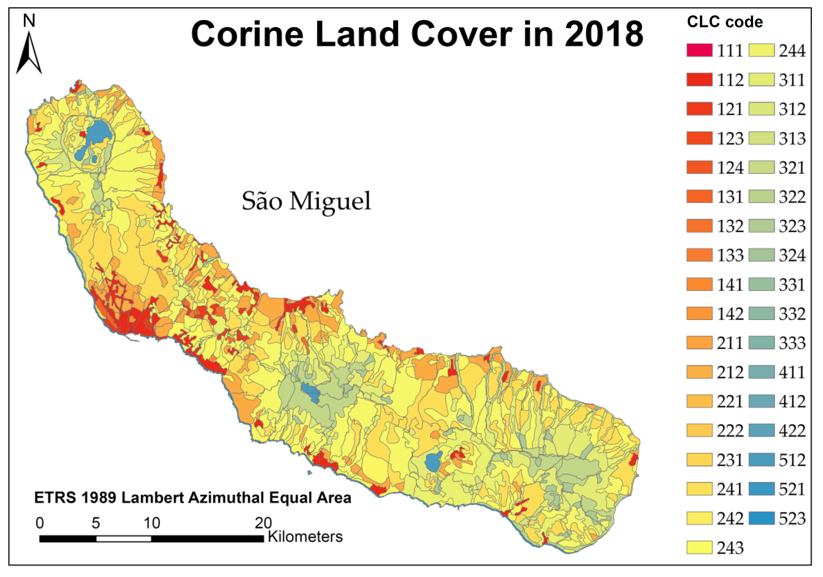
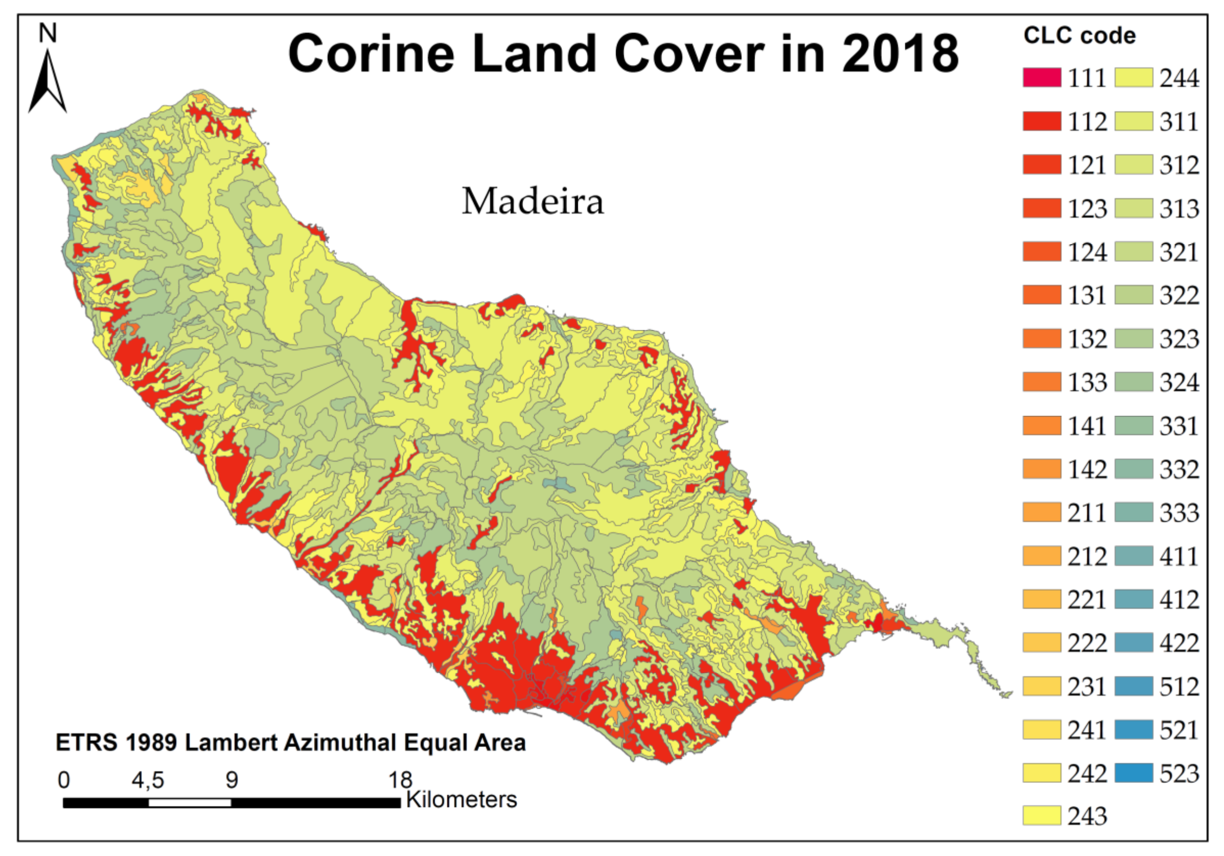
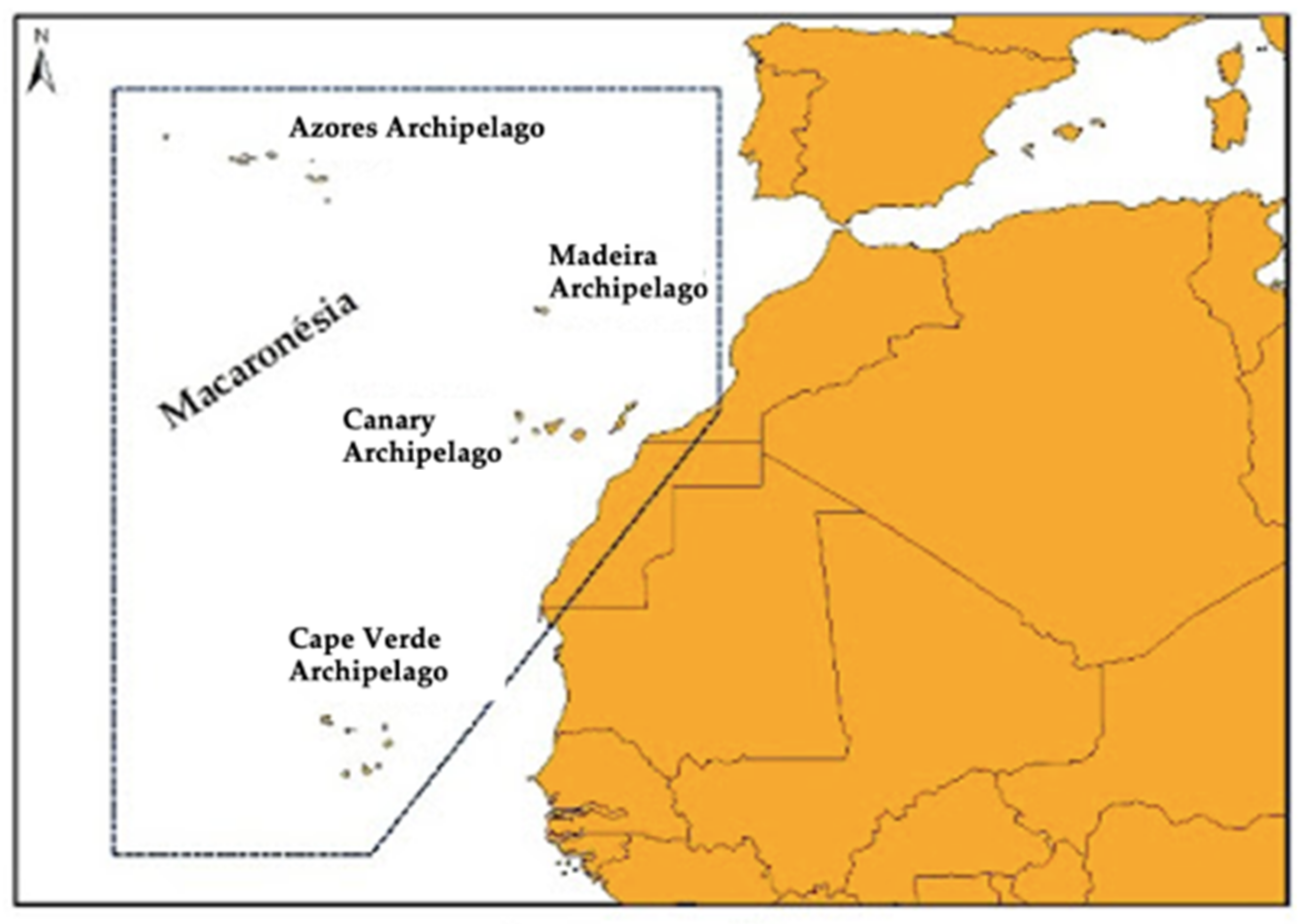
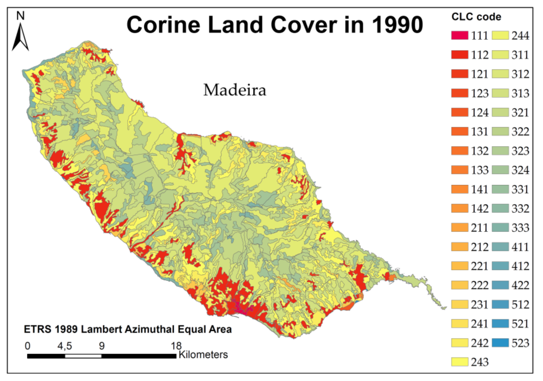
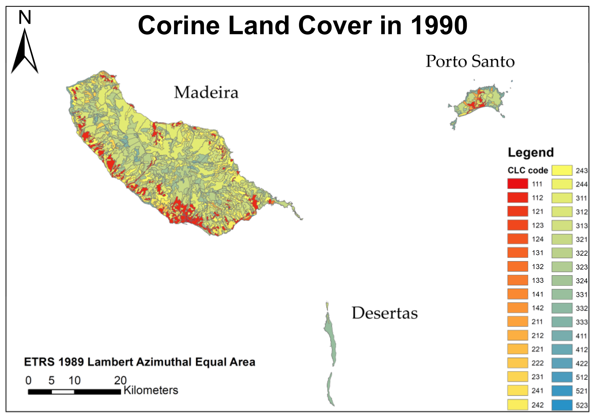
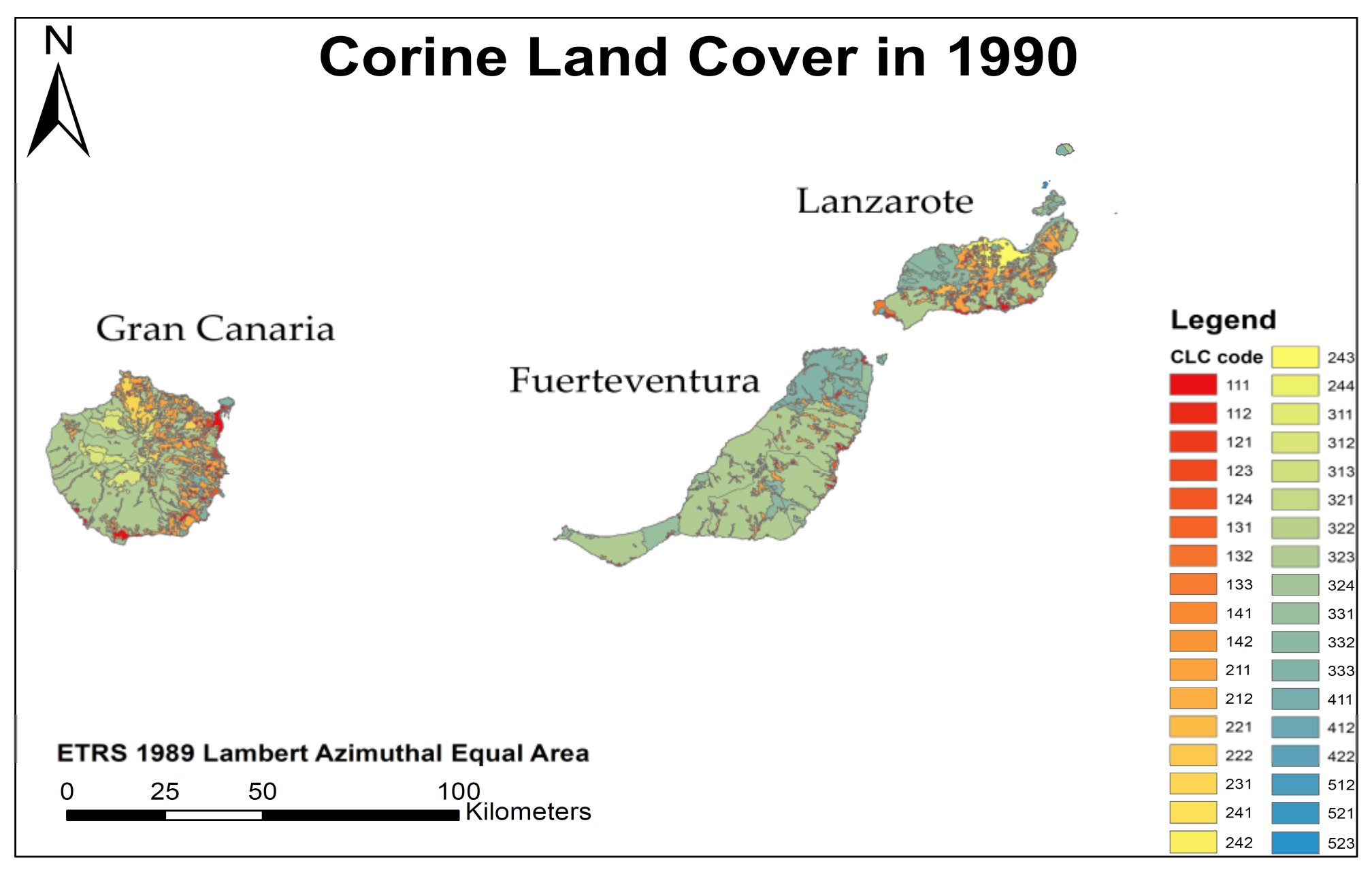
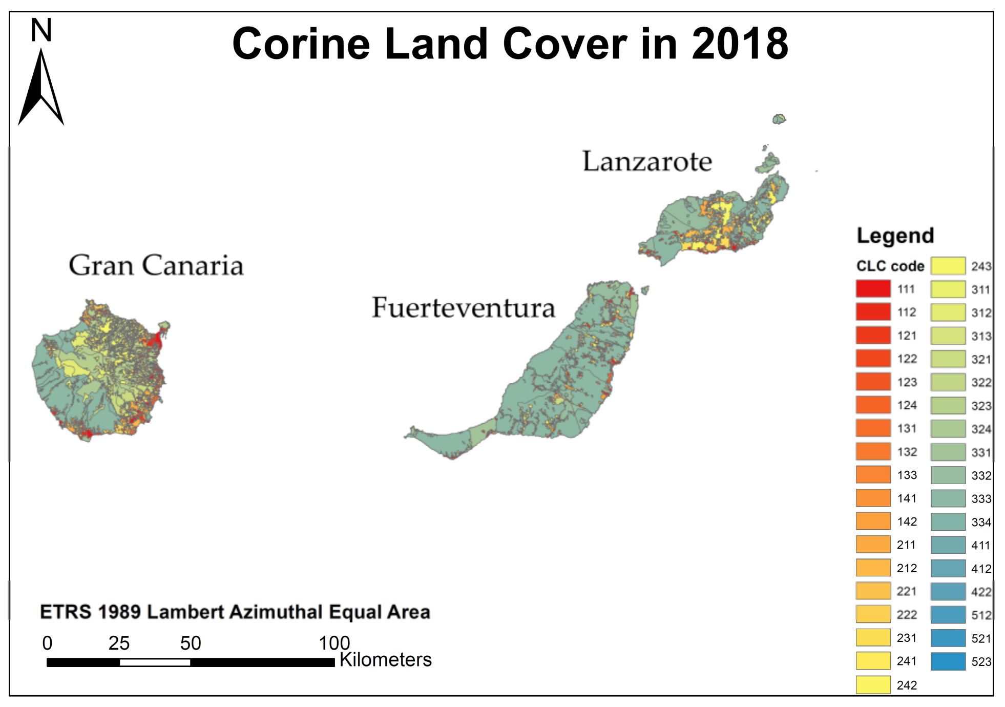
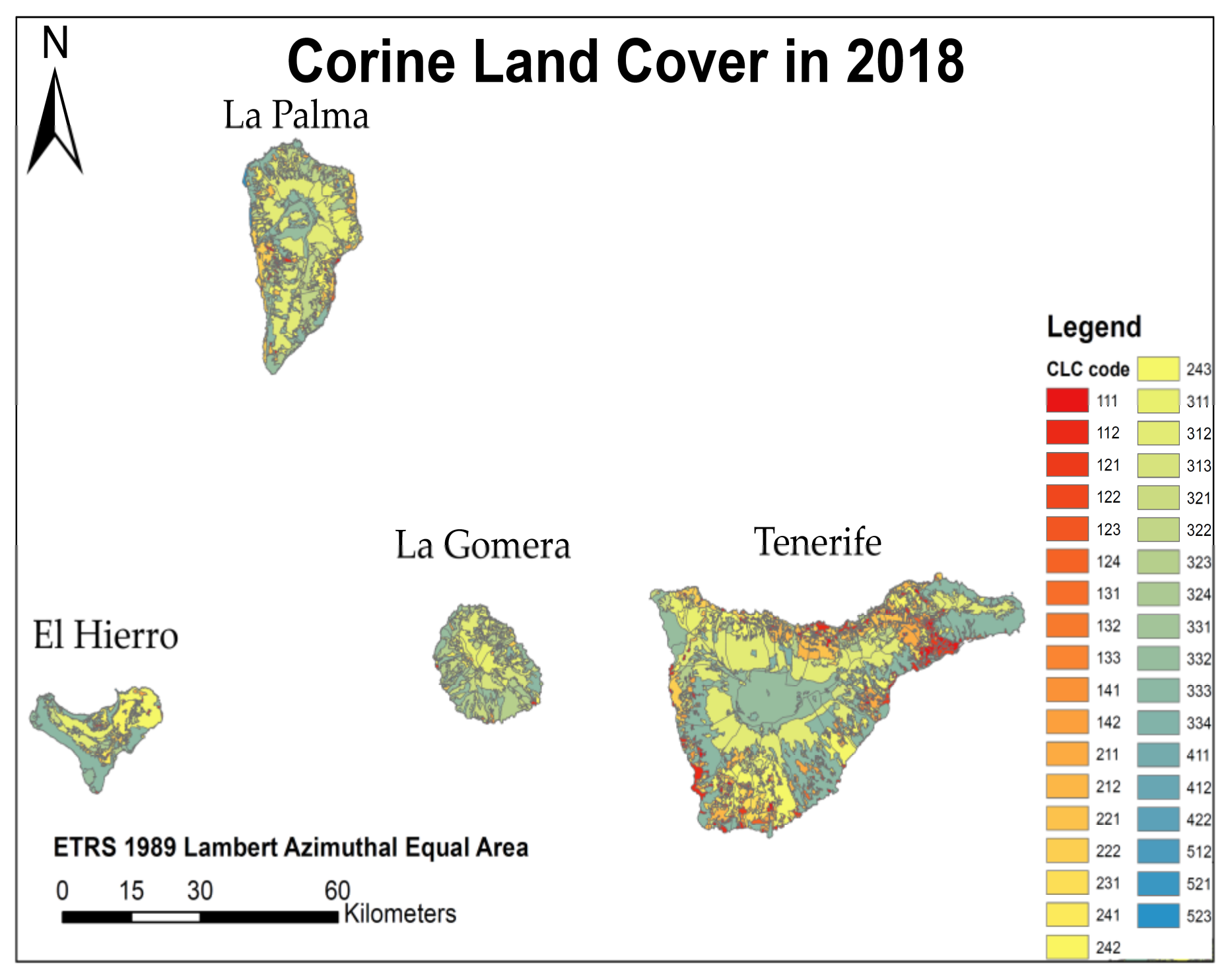
3.1. The Macaronesia Region

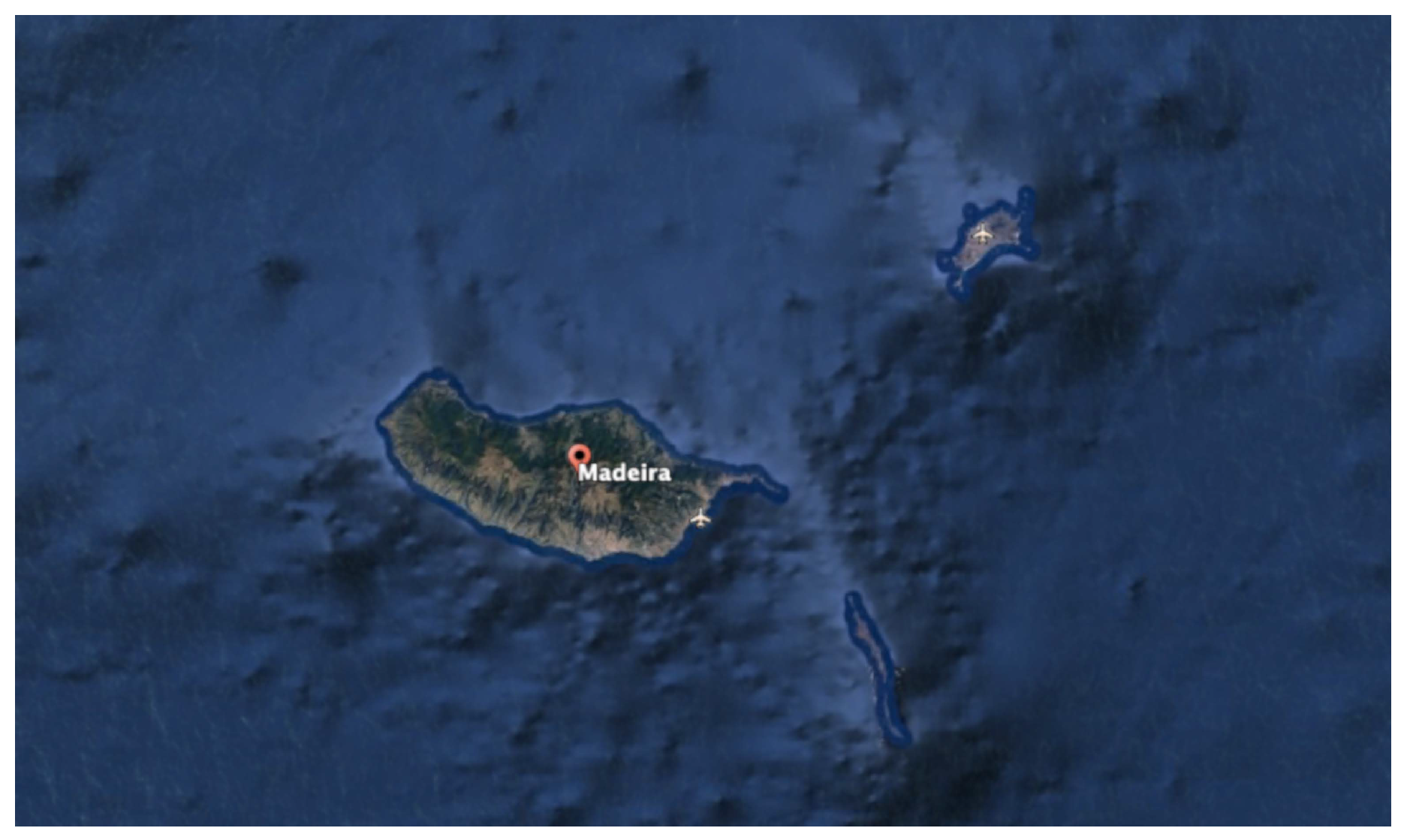
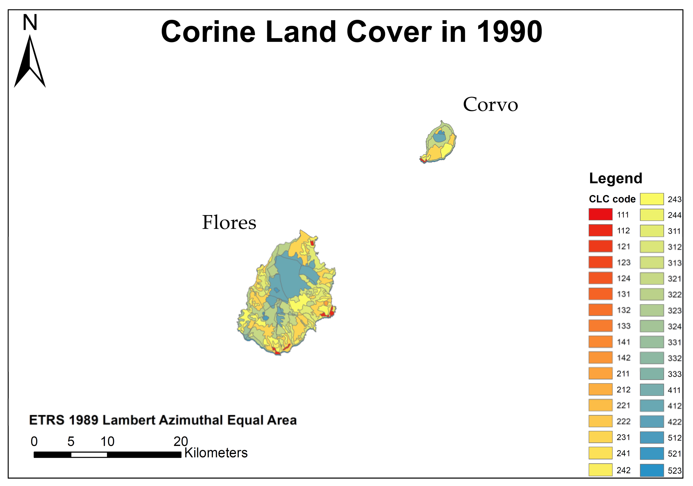
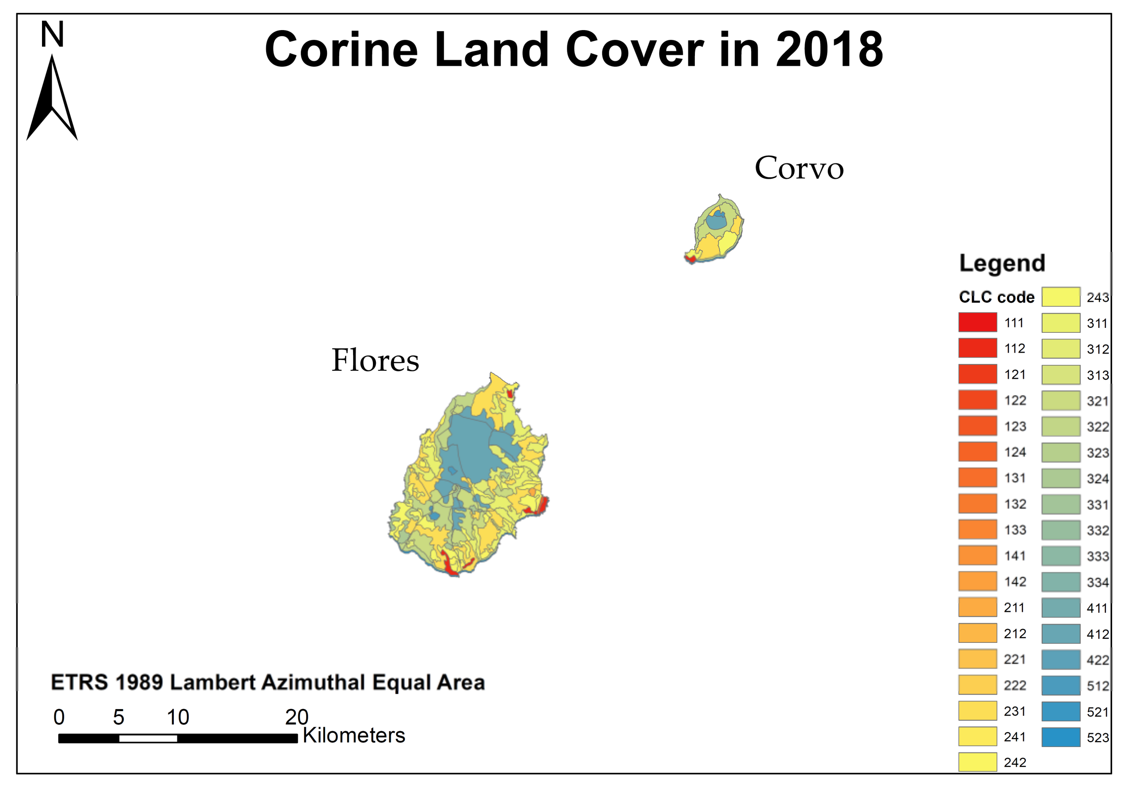
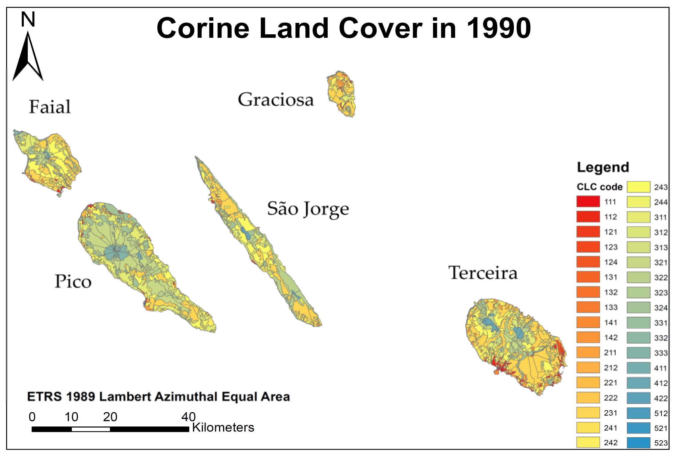
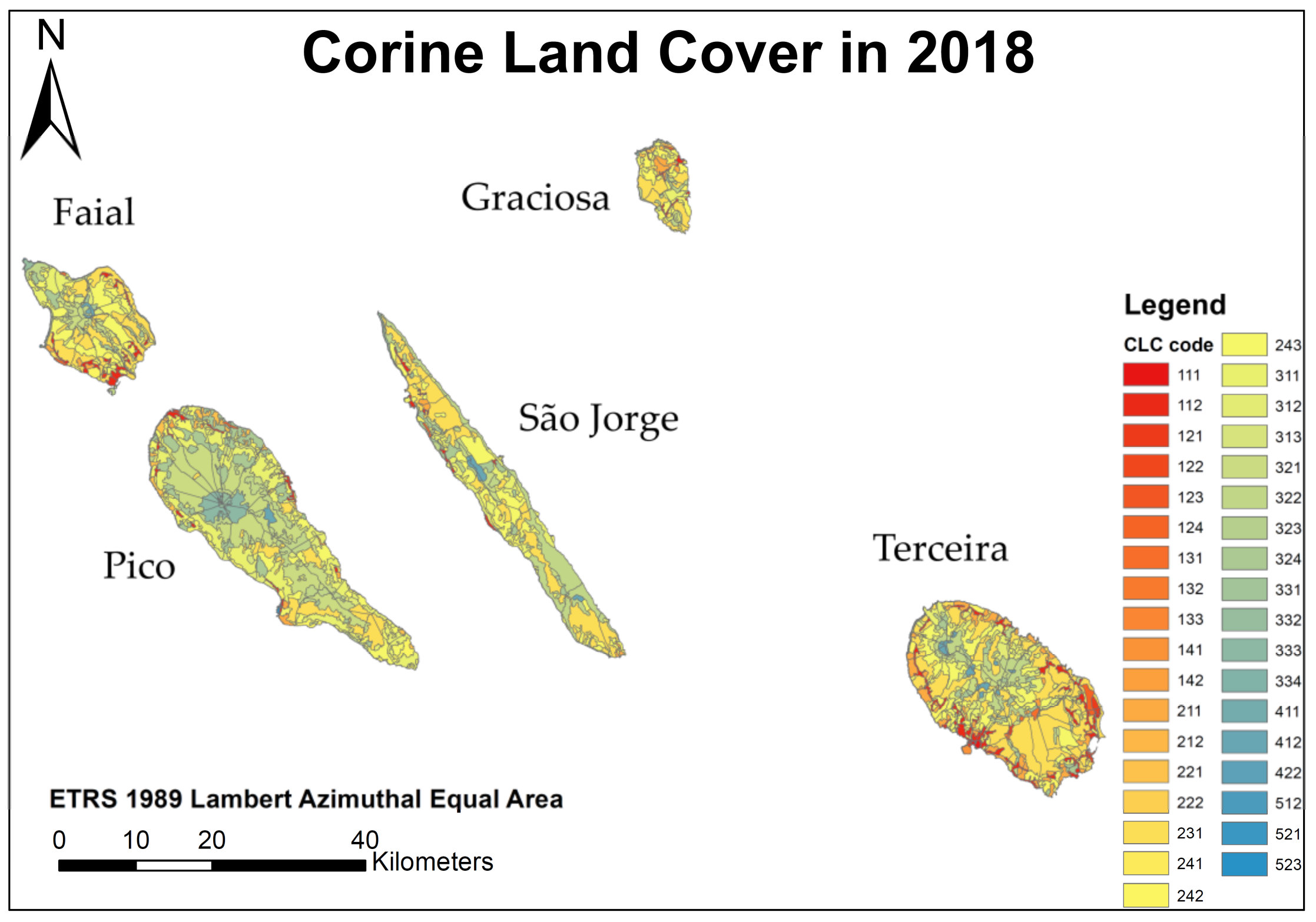
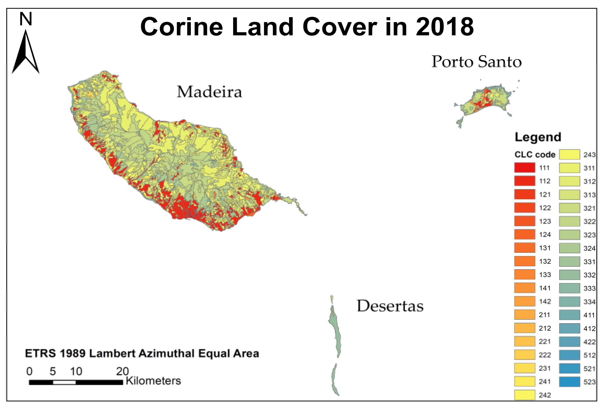
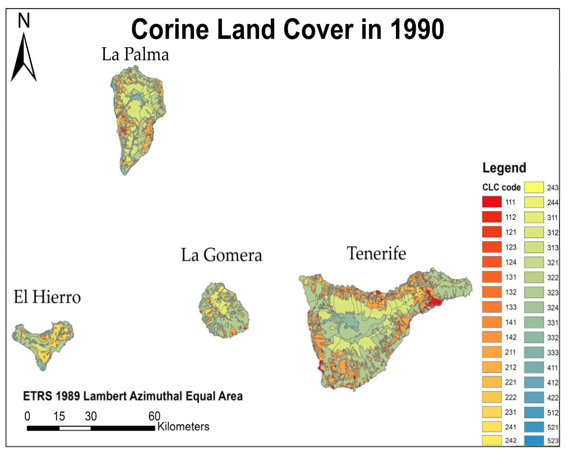
The three archipelagos (Figure 1, Figure 2 and Figure 3) share regional features: a volcanic origin, a contrasting landscape, and a gentle climate. These features have created an ideal environment for vibrant biodiversity [51]. The name Macaronesia is derived from the Greek words meaning "islands of the fortunate." Ancient Greek geographers first used the name to refer to any islands west of the Strait of Gibraltar. Macaronesia is a collection of four volcanic archipelagos in the North Atlantic Ocean, off Europe and Africa. Each archipelago is made up of several Atlantic oceanic islands formed by seamounts on the ocean floor and have peaks above the ocean’s surface.

Some of the Macaronesian islands belong to Portugal, some belong to Spain, and the rest belong to Cape Verde. Geologically, Macaronesia is part of the African tectonic plate. Some of its islands—the Azores—are situated along the edge of that plate when it abuts the Eurasian and North American plates. According to the European Environment Agency, the three European archipelagos constitute a unique biogeographic realm known as the Macaronesian Region (Figure 4). Entirely volcanic, the Macaronesian islands share a gentle climate and offer a wide variety of landscapes. The large calderas, jagged mountains and cliffs, broad valleys, and sheltered bays are home to various species and habitats. The islands may represent a mere 0.3% of the EU territory, but they host 19% of the habitat types and 28% of all the plants listed in the Habitats Directive [51].

Macaronesian islands are volcanic in origin and are thought to be the product of several geologic hotspots. The Macaronesian islands represent a wide range of climates. The annual average maximum temperatures in the Canary Islands range from 24 °C in coastal areas to values below 10 °C in the Pico de Teide. The annual average maximum air temperature in the Azores and Madeira is between 12 °C and 14 °C in higher altitudes and below 8 °C in Ponta do Pico on Pico Island in the Azores. The highest maximum air temperature values in the Azores, above 20 °C, occur in some coastal areas of São Miguel, Santa Maria, Terceira, Graciosa, and Pico. In Madeira, the highest average maximum air temperature values are also above 20 °C in coastal regions of Madeira and in almost the entire island of Porto Santo, where values are even higher than 22 °C in the southern and north-western coastal strip of the island of Madeira [53,54,55,56,57,58].

There are maritime temperate, the Mediterranean, and subtropical climates in the Azores and Madeira; the Mediterranean and subtropical climates in some of the Canary Islands; arid climates in certain geologically older islands of the Canaries (notably Lanzarote and Fuerteventura) and some of the islands of the Madeira Archipelago (Selvagens and Porto Santo) and Cape Verde (Sal, Boa Vista, and Maio); and a tropical climate in the younger islands of both of the southernmost archipelagos (Santo Antão, Santiago, and Fogo in Cape Verde). In some locations, there are variations in climate due to the rain shadow effect. Macaronesia’s laurisilva forests are a type of mountain cloud forest [51] with relict plant species of a vegetation type that originally covered much of the Mediterranean Basin when the climate of that region was more humid. Many of these plant species are endemic and have evolved to adapt to the islands’ variable climatic conditions. For example, the Laurisilva of Madeira is the largest surviving relict of a virtually extinct laurel forest type, once widespread in Europe. It is still 90% primary forest and is a center of plant diversity, containing a unique suite of rare and relict plants and animals, especially endemic bryophytes, ferns, vascular plants, and animals, the Madeiran long-toed pigeon, and a vibrant invertebrate fauna [59,60].

Much of the original native vegetation has been displaced because of human activity, including felling forests for timber and firewood, clearing vegetation for grazing and agriculture, and introducing foreign plants and animals into the islands. The laurisilva habitat has been reduced to small disconnected pockets. As a result, many of the endemic biotas of the islands are now seriously endangered or extinct.

Since 2001, the European Union’s conservation efforts, mandated by its Natura 2000 regulations [51], have protected large stretches of land and sea in the Azores, Madeira, and the Canary Islands, totaling 5000 km².

All archipelagos are outermost regions that are far from the countries or continent to which they belong, which requires special treatment to achieve the connection and development of these territories’ economies.

The European Archipelagos of Macaronesia Region

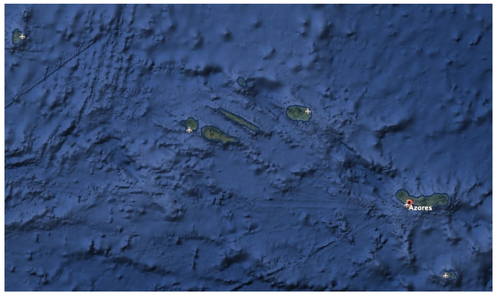
Azores

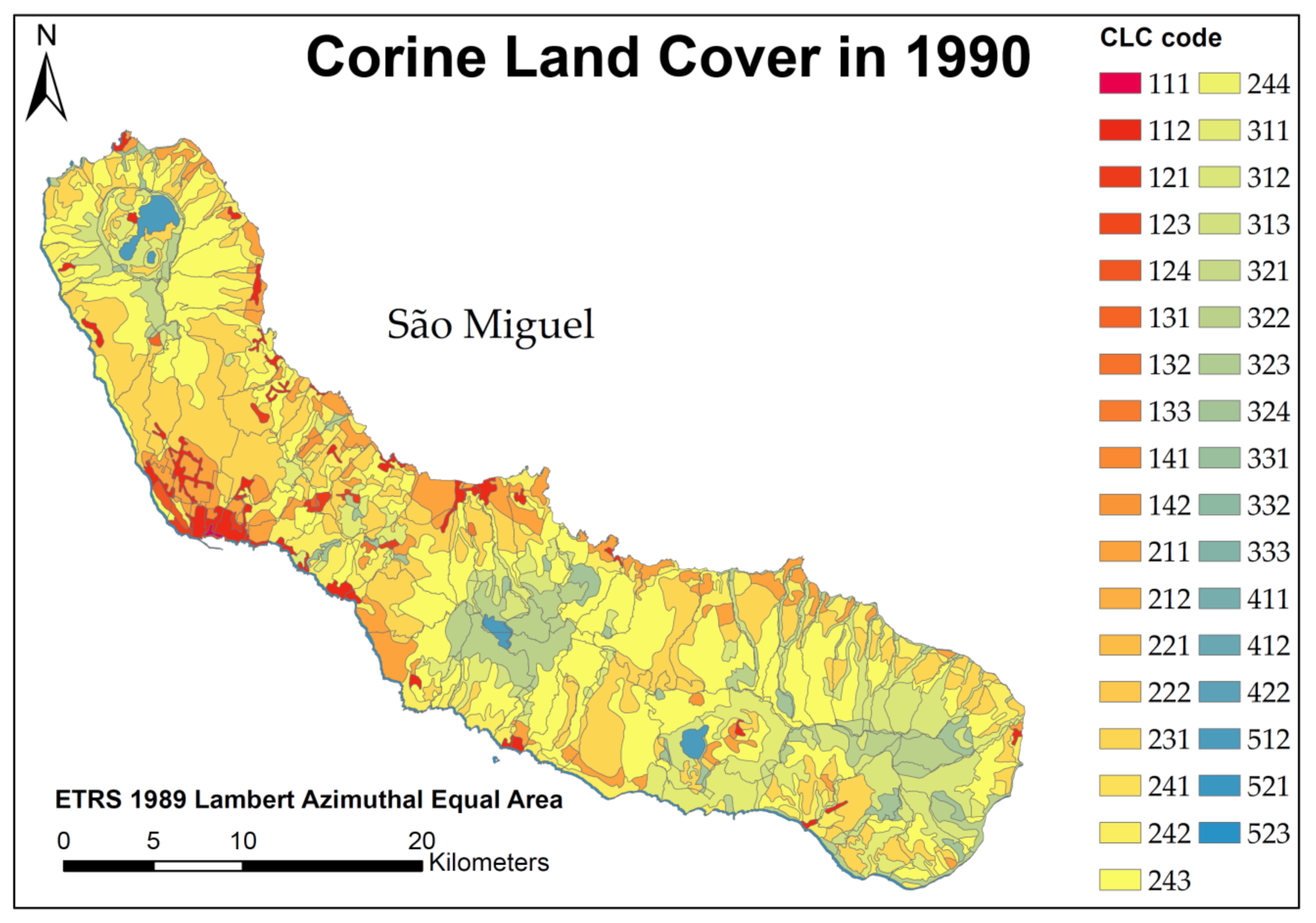
The Azores are an archipelago formed by nine islands, which constitute an autonomous region of Portugal. Its official language is Portuguese, and it has approximately 250,000 inhabitants in its 2.333 square kilometers of land. The largest island is São Miguel, where more than half of the Azores archipelago population is gathered, whose main city is Ponta Delgada.

The Azorean climate, relief, and rich soils are particularly suitable for agriculture, and the islands are now heavily deforested: only 2% of the original laurel forests remain [40]. The endemic Azores bullfinch (Pyrrhula murina) was once a common feature of the native forests and saw its population plummet to 120 pairs. However, it is now on the road to recovery thanks to an EU LIFE project that has now caused the population to treble [51].

Madeira

It is an archipelago that is part of Portugal, formed by only two inhabited islands, Madeira and Porto Santo, with more than 260,000 inhabitants in an extension of 828 square kilometers. Three smaller islands that are not inhabited are also part of the archipelago.

Agriculture is the mainstay of Madeira’s economy but has remained mainly small-scale due to the rugged landscape. Tourism is becoming increasingly important, generating 10% of the island’s GDP and employing a significant proportion of the 250,000 islanders [51].

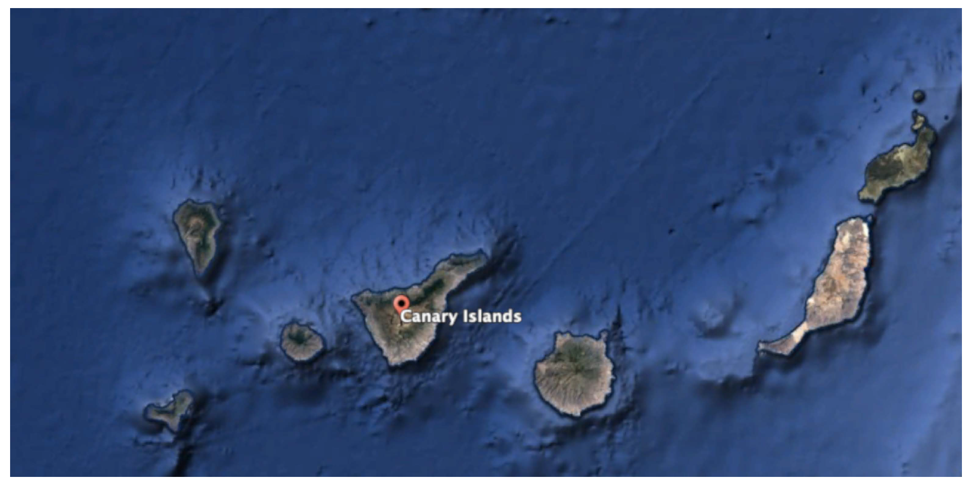
Canary Islands

The Canary Islands are formed by seven islands, subdivided into two provinces, being one of Spain’s autonomous communities. On the archipelago’s whole lives approximately 2,200,000 people in an extension of 7500 square kilometers, the most populated island being that of Gran Canaria, followed by Tenerife.

Tourism is the most important economic activity. Mixed and terraced farming is still practiced inland but has rapidly disappeared, replaced by the tropical and forced crops for the export market, accounting for 75% of the agricultural end production; 18,000 ha of highly fragmented laurel forest remain. Only 6000 ha correspond to mature forest [51].

4. Results

Bearing in mind the land occupation analyzed categories, it was possible to group the results. In the first phase, the number of land-uses has been defined in each of the studied years for each of the European Archipelagos of Macaronesia Region (Section 4.1, Section 4.2 and Section 4.3). After, in Section 4.4, it is conceivable to comprehend how the archipelagos’ land-use change dynamics could be associated among them.

4.1. The Azores Archipelago

This section presents the analysis of the most relevant and specific land-uses in the Azores archipelago (

Table 2. Percentage of land-uses according to level 1 of CLC nomenclature in the Autonomous Region of the Azores.

CODE	1990	2000	2006	2012	2018
1. Artificial surfaces	2.90%	3.41%	4.98%	5.13%	5.22%
2. Agricultural areas	57.17%	56.34%	54.43%	54.22%	54.62%
3. Forests and semi-natural areas	36.04%	36.38%	36.72%	36.78%	36.55%
4. Wetlands	2.36%	2.33%	2.33%	2.33%	2.08%
5. Water bodies	1.54%	1.54%	1.54%	1.54%	1.53%

The highest values found are in bold.

and

Table 3. Percentage of land-uses according to level 3 of CLC nomenclature in the Autonomous Region of the Azores.

CODE	1990	2000	2006	2012	2018	2018–1990
111	0.05%	0.05%	0.05%	0.05%	0.05%	0.00%
112	1.86%	2.16%	3.63%	3.71%	3.77%	1.91%
121	0.24%	0.35%	0.37%	0.44%	0.45%	0.21%
122	0.00%	0.00%	0.00%	0.00%	0.00%	0.00%
123	0.04%	0.04%	0.03%	0.04%	0.04%	0.00%
124	0.44%	0.44%	0.45%	0.46%	0.47%	0.03%
131	0.07%	0.11%	0.15%	0.16%	0.18%	0.11%
132	0.01%	0.07%	0.04%	0.04%	0.03%	0.02%
133	0.01%	0.03%	0.05%	0.01%	0.01%	0.00%
141	0.07%	0.07%	0.07%	0.07%	0.07%	0.00%
142	0.10%	0.10%	0.13%	0.15%	0.14%	0.04%
211	3.87%	3.83%	4.03%	4.11%	4.98%	1.11%
212	0.00%	0.00%	0.00%	0.00%	0.00%	0.00%
213	0.00%	0.00%	0.00%	0.00%	0.00%	0.00%
221	0.59%	0.35%	0.35%	0.35%	0.63%	0.04%
222	0.01%	0.01%	0.01%	0.01%	0.01%	0.00%
231	24.83%	24.56%	24.96%	24.74%	24.73%	−0.10%
241	0.00%	0.00%	0.00%	0.00%	0.00%	0.00%
242	7.25%	6.92%	6.12%	6.13%	5.80%	−1.45%
243	20.62%	20.67%	18.96%	18.89%	18.47%	−2.15%
244	0.00%	0.00%	0.00%	0.00%	0.00%	0.00%
311	9.36%	9.57%	9.40%	9.38%	9.88%	0.52%
312	3.63%	4.10%	4.35%	4.45%	4.11%	0.48%
313	0.89%	0.95%	1.02%	1.02%	1.01%	0.12%
321	8.02%	7.97%	7.87%	7.76%	7.38%	−0.64%
322	8.65%	8.63%	8.42%	8.42%	9.10%	0.45%
323	0.00%	0.00%	0.00%	0.00%	0.00%	0.00%
324	4.41%	4.08%	4.62%	4.72%	4.10%	−0.31%
331	0.00%	0.00%	0.00%	0.00%	0.00%	0.00%
332	0.25%	0.25%	0.25%	0.25%	0.25%	0.00%
333	0.82%	0.82%	0.79%	0.78%	0.72%	−0.10%
334	0.00%	0.00%	0.00%	0.00%	0.00%	0.00%
411	0.02%	0.02%	0.02%	0.02%	0.02%	0.00%
412	2.34%	2.32%	2.32%	2.31%	2.06%	−0.28%
422	0.00%	0.00%	0.00%	0.00%	0.00%	0.00%
512	0.40%	0.40%	0.40%	0.40%	0.40%	0.00%
521	0.00%	0.00%	0.00%	0.00%	0.00%	0.00%
523	1.13%	1.13%	1.13%	1.13%	1.13%	0.01%

The highest values found are in bold.

, and Figure 5, Figure 6, Figure 7 and Figure 8).

By analyzing Table 2 and Figure 5, it is possible to verify the significant increase in the artificial surfaces (Code 1) in the Azores Region between 1990 and 2018. In fact, the variation of this land occupation around 2.30%. Additionally, the decrease in agricultural areas in the period 1990–2018 is evident—with a variation of 2.55%. A slight increase was noticed in forests and semi-natural areas—a reduction of 0.23% if we consider the highest value in 2012 to the present. A decreased tendency is also found in the land occupation related to wetlands—with a decrease of 0.28%, between 1990 to 2018. Furthermore, an insignificant decrease was identified regarding the water bodies from 1990 to 2018—a variation of 0.01%.

In Table 3 and Figure 6, it is possible to analyze in detail the land-use changes in the Azores Autonomous Region. In this regard, if we consider the period between 1990 and 2018, the most significant difference occurs in CLC-243 (Land principally occupied by agriculture, with significant natural vegetation areas) with a reduction of 2.15%. The second significant difference occurs in CLC-112 (Discontinuous urban fabric), with an increase of 1.91%. The third significant difference corresponds to CLC-242 (Complex cultivation) with a reduction of 1.45%. Finally, the fourth significant difference falls on CLC-211 (Non-irrigated arable land), increasing 1.11%. Besides these, we have CLC-121 (Industrial or commercial units), CLC-124 (Airports), CLC-131 (Mineral extraction sites), CLC-211 (Non-irrigated arable land)—with variations of 1.91%, 0.21%, 0.03%, 0.11%, and 1.11%, respectively. On the other hand, it is also possible to identify other important reductions in the land-use over the years in the Azores Archipelago, as is the case of CLC-133 (Construction sites) and CLC-312 (Coniferous forest)—with decreases of 0.04%, 2.20%, and 0.34%.

For a more accurate analysis of the results, thematic cartography was created for the three regions within the Azorean Archipelago (Western, Central, and Eastern), for the initial period (1990) and the last period (2018) (Appendix A). The following shows the thematic cartography for the Eastern Group of Azores Archipelago, once it is where the Capital Island (São Miguel) is located (Figure 7 and Figure 8).

4.2. The Madeira Archipelago

This section presents the analysis of the most relevant and specific land-uses in the Madeira Archipelago (

Table 4. Percentage of land-uses according to level 1 of CLC nomenclature in the Autonomous Region of Madeira.

CODE	1990	2000	2006	2012	2018
1. Artificial surfaces	10.11%	14.30%	15.20%	15.21%	14.96%
2. Agricultural areas	19.41%	16.25%	14.26%	14.29%	13.83%
3. Forests and semi-natural areas	69.45%	68.45%	70.12%	70.08%	70.80%
4. Wetlands	0.00%	0.00%	0.00%	0.00%	0.00%
5. Water bodies	1.02%	1.00%	0.42%	0.42%	0.41%

The highest values found are in bold.

and

Table 5. Percentage of land-uses according to CLC nomenclature in the Autonomous Region of Madeira.

CODE	1990	2000	2006	2012	2018	2018–1990
111	0.21%	0.21%	0.30%	0.30%	0.32%	0.11%
112	9.43%	13.05%	13.44%	13.48%	13.16%	3.73%
121	0.09%	0.22%	0.35%	0.40%	0.43%	0.34%
122	0.00%	0.04%	0.04%	0.04%	0.04%	0.04%
123	0.02%	0.03%	0.03%	0.03%	0.04%	0.02%
124	0.25%	0.30%	0.30%	0.30%	0.30%	0.05%
131	0.00%	0.00%	0.15%	0.15%	0.15%	0.15%
132	0.00%	0.04%	0.08%	0.06%	0.06%	0.06%
133	0.07%	0.15%	0.13%	0.06%	0.06%	-0.01%
141	0.04%	0.04%	0.04%	0.04%	0.04%	0.00%
142	0.00%	0.21%	0.32%	0.35%	0.36%	0.36%
211	0.15%	0.15%	0.04%	0.04%	0.04%	−0.11%
212	0.48%	0.48%	0.04%	0.04%	0.04%	−0.44%
213	0.00%	0.00%	0.00%	0.00%	0.00%	0.00%
221	0.17%	0.17%	0.18%	0.21%	0.19%	0.02%
222	0.74%	0.45%	0.31%	0.31%	0.31%	−0.43%
231	0.95%	0.92%	0.34%	0.34%	0.51%	−0.44%
241	0.94%	0.92%	0.25%	0.25%	0.00%	−0.94%
242	4.94%	3.14%	2.83%	2.80%	3.42%	−1.52%
243	10.80%	9.56%	10.28%	10.32%	9.33%	−1.47%
244	0.24%	0.45%	0.00%	0.00%	0.00%	−0.24%
311	20.42%	20.21%	20.43%	18.92%	18.64%	−1.78%
312	5.79%	5.64%	5.20%	4.65%	4.12%	−1.67%
313	14.06%	13.81%	13.00%	11.86%	10.60%	−3.46%
321	9.03%	8.88%	9.79%	9.42%	9.78%	0.75%
322	10.78%	10.70%	11.01%	9.33%	16.40%	5.62%
323	0.00%	0.00%	0.00%	0.00%	0.00%	0.00%
324	6.52%	6.30%	6.22%	5.56%	7.85%	1.33%
331	0.12%	0.12%	0.12%	0.12%	0.06%	−0.06%
332	0.30%	0.30%	1.85%	1.85%	1.85%	1.55%
333	2.42%	2.42%	2.27%	2.27%	1.47%	−0.95%
334	0.00%	0.06%	0.23%	6.09%	0.04%	0.04%
411	0.00%	0.00%	0.00%	0.00%	0.00%	0.00%
412	0.00%	0.00%	0.00%	0.00%	0.00%	0.00%
422	0.00%	0.00%	0.00%	0.00%	0.00%	0.00%
512	0.00%	0.00%	0.00%	0.00%	0.00%	0.00%
521	0.00%	0.00%	0.00%	0.00%	0.00%	0.00%
523	1.02%	1.00%	0.42%	0.42%	0.41%	−0.61%

The highest values found are in bold.

, Figure 9, Figure 10, Figure 11 and Figure 12, and Appendix B).

Throughout the analysis of Table 4 and Figure 9, it is possible to find an increase of 4.85% in the artificial surfaces (between 1990 and 2018) in the Madeira Region; however, the highest results were identified in 2012 with more than 0.25% of the surface in comparison with the current period. Additionally, another increase is noticed in forests and semi-natural areas—showing a variation of 1.35%, if we consider the initial period (1990) and the final period (2018). Moreover, the results show a significant reduction of 5.58% in the agricultural surfaces (from 1990 to 2018). Another decrease was found in the land cover classified as water bodies, with a reduction of 0.61% (between 1990 and 2018).

Table 5 and Figure 10 show with greater detail the land-use changes in the Madeira Autonomous Region. Contextually, if we consider the period between 1990 and 2018, the most significant differences in land-use are CLC-322 (Moors and heathland) and CLC-112 (Discontinuous urban fabric) 5.62% and 3.73%, respectively. On the contrary, the most significant decreases are for land-uses of CLC-313 (Mixed forest) and CLC-311 (Broad-leaved forest), with 3.46% and 1.78%, respectively. Besides, the obtained results evidence considerable increases in the surfaces of land occupations in CLC-111 (Continuous urban fabric), CLC-121 (Industrial or commercial units), CLC-131 (Mineral extraction sites), CLC-142 (Sport and leisure facilities), CLC-324 (Transitional woodland shrub), and CLC-332 (Bare rock)—with variations of 0.11%, 0.34%, 0.15%, 0.36%, 5.62%, 1.33%, and 1.55%, respectively. Contrarily, if we focus on the period between 1990 and 2018, it is also possible to find concerning reductions in the land-use over the years in the Madeira Region, as is the case of CLC-222 (Fruit trees and berry plantations), CLC-231 (Pastures), CLC-241 (Annual crops associated with permanent crops), CLC-242 (Complex cultivation), CLC-243 (Land occupied by agriculture), CLC-312 (Coniferous forest), and CLC-523 (Sea and ocean)—with decreases of 0.43%, 0.44%, 0.94%, 1.80%, 1.47%, 1.67%, 3.46%, and 0.61%. Additionally, other reductions should be highlighted as is the case of the CLC-211 and CLC-212 and CLC-333 (from 2000 to 2018); and CLC-334 (from 2012 to 2018).

Additionally, with the results, thematic cartography was created for the Madeira Island for the initial period (1990) and the last period (2018) (Appendix B and Figure 11 and Figure 12).

4.3. The Canary Archipelago

The current section shows the obtained outcomes of the most relevant and specific land-uses in the Canary Archipelago (

Table 6. Percentage of land-uses according to level 1 of CLC nomenclature in the Autonomous Community of the Canary Islands.

CODE	1990	2000	2006	2012	2018
1. Artificial surfaces	4.14%	4.50%	6.05%	6.11%	6.23%
2. Agricultural areas	22.63%	22.59%	16.52%	16.51%	19.99%
3. Forests and semi-natural areas	72.12%	71.79%	76.35%	76.29%	72.69%
4. Wetlands	0.00%	0.00%	0.00%	0.00%	0.00%
5. Water bodies	1.10%	1.10%	1.07%	1.07%	1.08%

The highest values found are in bold.

and

Table 7. Percentage of land-uses according to CLC nomenclature in the Autonomous Community of the Canary Islands.

CODE	1990	2000	2006	2012	2018	2018–1990
111	2.20%	2.45%	1.40%	1.42%	1.39%	−0.81%
112	0.85%	0.89%	2.57%	2.63%	3.01%	2.16%
121	0.24%	0.36%	0.57%	0.61%	0.70%	0.46%
122	0.00%	0.01%	0.00%	0.00%	0.05%	0.05%
123	0.06%	0.07%	0.09%	0.09%	0.09%	0.03%
124	0.17%	0.18%	0.23%	0.23%	0.22%	0.05%
131	0.15%	0.16%	0.25%	0.25%	0.29%	0.14%
132	0.01%	0.01%	0.02%	0.01%	0.02%	0.01%
133	0.36%	0.28%	0.60%	0.51%	0.11%	−0.25%
141	0.02%	0.02%	0.03%	0.03%	0.03%	0.01%
142	0.07%	0.09%	0.29%	0.32%	0.34%	0.27%
211	13.44%	13.37%	3.19%	3.18%	3.14%	−10.30%
212	1.14%	1.20%	2.40%	2.40%	1.77%	0.63%
213	0.00%	0.00%	0.00%	0.00%	0.00%	0.00%
221	2.15%	2.16%	1.33%	1.33%	1.34%	−0.81%
222	1.75%	1.71%	2.07%	2.07%	1.85%	0.10%
231	3.25%	3.24%	2.07%	2.05%	1.97%	−1.28%
241	0.00%	0.00%	0.12%	0.12%	0.11%	0.11%
242	0.00%	0.00%	1.20%	1.20%	2.45%	2.45%
243	0.91%	0.91%	4.15%	4.15%	7.35%	6.44%
244	0.00%	0.00%	0.00%	0.00%	0.00%	0.00%
311	1.36%	1.36%	2.49%	2.49%	2.46%	1.10%
312	10.48%	10.46%	11.21%	11.08%	11.03%	0.55%
313	0.00%	0.00%	0.47%	0.47%	0.59%	0.59%
321	0.00%	0.00%	2.01%	2.01%	2.63%	2.63%
322	2.99%	2.99%	0.38%	0.38%	1.07%	−1.92%
323	44.95%	44.69%	15.75%	15.72%	7.26%	−37.69%
324	0.00%	0.00%	0.81%	0.90%	1.41%	1.41%
331	1.68%	1.68%	1.75%	1.75%	1.63%	−0.05%
332	4.87%	4.87%	10.57%	10.57%	10.51%	5.64%
333	5.78%	5.75%	30.78%	30.76%	33.92%	28.14%
334	0.00%	0.00%	0.12%	0.18%	0.18%	0.18%
411	0.00%	0.00%	0.00%	0.00%	0.00%	0.00%
412	0.00%	0.00%	0.00%	0.00%	0.00%	0.00%
422	0.01%	0.01%	0.01%	0.01%	0.01%	0.00%
512	0.01%	0.01%	0.02%	0.02%	0.02%	0.01%
521	0.00%	0.00%	0.00%	0.00%	0.00%	0.00%
523	1.09%	1.09%	1.05%	1.05%	1.05%	−0.04%

The highest values found are in bold.

, Figure 13, Figure 14, Figure 15 and Figure 16, and Appendix C).

Table 6 and Figure 13 show the highest increase (2.09%) in the artificial surfaces (between 1990 and 2018) in the Canary Islands. Moreover, in forests and semi-natural areas, another increase was verified—with a variation of 0.57% (in the period 1990–2018). If we focus on reducing land occupation in the same periods, the most significant decrease was identified in agricultural areas (reducing 2.64%). In this sense, there was also a reduction of 0.02% in water bodies from 1990 to 2018.

Contextually, through the analysis of Table 7 and Figure 14, we can perceive the land-use changes in the Canary Archipelago with greater detail. Regarding the period between 1990 and 2018, the most significant differences are produced by a considerable reduction of 37.69% in CLC-323 (Sclerophyllous vegetation) and 10.30% in CLC-211 (Non-irrigated arable land). However, a considerable increase of 28.14% corresponds to CLC-333 (Sparsely vegetated areas) followed by a 6.44% increase equivalent to CLC-243 (Land principally occupied by agriculture). Besides, the collected results show substantial increases in the surfaces of land occupations CLC-112 (Discontinuous urban fabric), in CLC-121 (Industrial or commercial units), CLC-131 (Mineral extraction sites), CLC-142 (Sport and leisure facilities), CLC-242 (Complex cultivation), CLC-313 (Mixed forest), CLC-321 (Natural grassland), CLC-324 (Transitional woodland shrub), and CLC-334 (Burnt areas)—with variations of 2.16%, 0.46%, 0.14%, 0.27%, 2.45%, 6.44%, 0.59%, 2.63%, 1.41%, 28.1%, and 0.18%, respectively. Contrarily, suppose we focus on the land-use cover reductions between 1990 and 2018 on this archipelago. In that case, it is possible to highlight the following CLC-231 (decrease of 1.28%). In this sense, if we consider the period between 2000–2018, some decreases in the land covers should be noticed, as CLC-111 (reduction of 1.06%), CLC-221 (reduction of 0.82%), and CLC-322 (reduction of 1.92%). Moreover, the reduction of 0.49% in CLC-133 (Dump sites) is evident between 2006 and 2018. Finally, between 2012 and 2018 there was also two other reductions in CLC-212 and CLC-222.

Furthermore, based on the results, thematic cartography was created for the Canary Islands for the initial period (1990) and the last period (2018) (Appendix C). Contextually, the thematic cartography for the most populated island of the Canary Archipelago, Tenerife, is shown (Figure 15 and Figure 16).

4.4. Land-Use Change Associations

The present section was created to further comprehend how the archipelagos’ land-use change dynamics could be associated.

Therefore, the correlation in the land-uses in each of the archipelagos was performed using the percentage land-use varies according to the CLC code by using R software.

Subsequently, considering a confidence level of 95% and n < 30, the normality of the data was verified using the Shapiro–Wilk test. The values obtained are less than 0.05; as a consequence, normality is discarded. Therefore, a non-parametric test was performed, with ordinal data, considering the covariation hypothesis to determine the Spearman correlation matrix—both for land-uses at level 1.

Based on the previous tables, the strength of negative or positive association between the variables corresponding to the percentage of surface intended for certain level 1 land-uses can be analyzed according to CLC between 1990 and 2018. Initially, it can be observed that the strength of the association is always equal to or greater than moderate (0.40–0.59); there are even strong correlation values (0.60–0.79), and very strong (0.80–1.00), whether we consider strong or very strong partnerships. Firstly, land-use in agricultural areas declined between 1990 and 2012, at 2.95%, equivalent to 6913.45 hectares, as land-uses identified as artificial surfaces and forest and semi-natural areas increased to 2.23% and 0.74%, equivalent to 5231.58 and 1746.21 hectares, respectively. Additionally, artificial surfaces increased slightly between 2012 and 2018, 0.09% equivalent to 214.73 hectares when water bodies were reduced—0.001%, 3.82 hectares. Secondly, artificial surfaces gradually increased throughout the period analyzed—2.32%, 5454.38 hectares, when forest and semi-natural areas decreased between 2012 and 2018—0.51%, 1200.46 hectares, and previously due to the loss of other land-uses. Thirdly, forest and semi-natural areas increased between 1990 and 2012—0.74%, 1746.21 hectares, when the extent of Artificial surfaces land-use increased—2,23%, 5239.65 hectares, over the same period. Fourthly, the surface of the water bodies remains virtually unchanged. Although, it descends slightly between 2012 and 2018—0.002% 4.01 hectares, due to the increase of artificial surfaces. Finally, wetlands have declined— 0.28%, 664.89 hectares, along those analyzed by the increase in artificial surfaces (

Table 8. Spearman’s rank correlation coefficient in the Azores Archipelago.

	Agr	Art	For	Wat	Wet	Acronym	CORINE Land Cover Nomenclature
Agr	1.0	−0.7	−1.0	0.7	0.5	Agr	Agricultural areas
Art	−0.7	1.0	0.7	−1.0	−0.9	Art	Artificial surfaces
For	−1.0	0.7	1.0	−0.7	−0.5	For	Forests and semi-natural areas
Wat	0.7	−1.0	−0.7	1.0	0.9	Wat	Water bodies
Wet	0.5	−0.9	−0.5	0.9	1.0	Wet	Wetlands

and Appendix D).

Regarding the Madeira Archipelago (

Table 9. Spearman’s rank correlation coefficient in the Madeira Archipelago.

	Agr	Art	For	Wat	Acronym	CORINE Land Cover Nomenclature
Agr	1.0	−0.9	−0.6	0.9	Agr	Agricultural areas
Art	−0.9	1.0	0.3	−0.7	Art	Artificial surfaces
For	−0.6	0.3	1.0	−0.8	For	Forests and semi-natural areas
Wat	0.9	−0.7	−0.8	1.0	Wat	Water bodies

and Appendix E), we have considered strong, and very strong relationships between variables, where the interpretation of Table 5 and

Table 10. Spearman’s rank correlation coefficient in the Canary Archipelago.

	Agr	Art	For	Wat	Wet	Acronym	CORINE Land Cover Nomenclature
Agr	1.0	−0.7	−0.8	1.0	−0.9	Agr	Agricultural areas
Art	−0.7	1.0	0.5	−0.7	0.9	Art	Artificial surfaces
For	−0.8	0.5	1.0	−0.8	0.6	For	Forests and semi-natural areas
Wat	1.0	−0.7	−0.8	1.0	−0.9	Wat	Water bodies
Wet	−0.9	0.9	0.6	−0.9	1.0	Wet	Wetlands

was performed. Firstly, agricultural areas have declined over the years analyzed—5.12%, 4099.94 hectares, when artificial surfaces have increased between 2000 and 2012—0.91%, 726.81 hectares, and forest and semi-natural areas between 2000 and 2006—1.67%, 1338.65 hectares, and between 2012 and 2018—0.72%, 578.45 hectares. Secondly, artificial surfaces would have been dwarfed between 2012 and 2018, and throughout the period analyzed, if the area of agricultural areas and water bodies had increased. However, these last two land-uses have been declining over the years analyzed—5.59% and 0.61%, 4477.59 and 488.12 hectares, respectively. Thirdly, forest and semi-natural areas have increased, as it would have decreased if agricultural areas and water bodies had increased. However, these land-uses have declined—5.59% and 0.61%, 4474.59 and 488.12 hectares, respectively. Finally, water bodies declined over the years and were analyzed mainly due to the increase in artificial surfaces—4.85%, 3882.34 hectares, and forest and semi-natural areas—1.35%, 1080.37 hectares.

Concerning the Canary Archipelago (Table 10 and Appendix F), firstly, agricultural areas declined in all the years analyzed—2.64%, 19,805.77 hectares, due to the increase in artificial surfaces—2.09%, 15,687.92 hectares, by increasing forest and semi-natural areas—4.55% 34,097.38 hectares, and wetlands—0.001%, 7.49 hectares, between 2000 and 2006. Although, the latter land-use was slightly increased and is not appreciable in Table 7 by using two decimal places. Secondly, artificial surfaces increased in all the years analyzed—2.09%, 15,687.92 hectares. Thirdly, forest and semi-natural areas increased between 2000 and 2006—4.22%, 31,646.37 hectares, and decreased between 2012 and 2018—3.60%, 26,984.02 hectares. Fourthly, water bodies were reduced between 2000 and 2018—0.02%, 182.96 hectares, as artificial surfaces increased—1.73%, 12,929.45 hectares, when forest and semi-natural areas increased between 2000 and 2006—4.55% 34,097 hectares, and between 2012 and 2018—0.12%, 867.34 hectares. Finally, wetlands remain virtually unchanged.

4.5. Results of Landscape Fragmentation Analysis

Regarding the results obtained from landscape fragmentation analysis (FRAGSTATS), it should be noted for the patch analysis level that Euclidean nearest-neighbor distance is perhaps the most straightforward patch context being used extensively to quantify patch isolation. Here, the nearest-neighbor distance is defined using simple Euclidean geometry as the shortest straight-line distance between the focal patch and its nearest-neighbor of the same class. ENN approaches 0 as the distance to the nearest- neighbor decreases. This index provides more information about the structure of the set and some of the vital importance in its dynamics and function. A decrease in its values can result in new fragments in the case of very isolated soil-uses. On the contrary, their increase can mean the aggregation of multiple fragments that were nearby.

The minimum ENN is constrained by the cell size and is equal to twice the cell size when the 8-neighbor patch rule is used. ENN is undefined and reported as “N/A” in the “basename”.patch file if the patch has no neighbors.

In the case of the Autonomous Region of Azores (Appendix G and

Table 11. Class metrics for the Autonomous Region of Azores.

1990				2018
TYPE	NP	SHAPE_MN	FRAC_MN	TYPE	NP	SHAPE_MN	FRAC_MN
111	2	1.9487	1.1032	111	2	1.9487	1.1032
112	155	2.0913	1.0951	112	112	2.324	1.1202
121	3	1.2476	1.0356	121	21	1.6568	1.0774
123	11	1.7607	1.0875	123	14	1.8397	1.0893
124	7	1.9395	1.0986	124	8	1.9887	1.1026
131	67	1.7617	1.0796	131	10	1.4863	1.0624
132	6	1.4548	1.0594	132	2	1.2541	1.0373
133	17	1.87	1.0911	133	1	1.5556	1.0716
141	98	1.7825	1.0829	141	3	1.2415	1.0352
142	7	1.5219	1.0607	142	7	1.4744	1.0591
211	226	1.9385	1.0906	211	121	1.6826	1.0753
221	1	1.8824	1.1049	221	23	1.8637	1.0919
222	1	1.2059	1.0321	222	1	1.8824	1.1049
231	21	1.9689	1.0934	231	179	2.0588	1.0945
242	110	1.621	1.0704	242	183	1.8611	1.0894
243	108	2.0105	1.094	243	244	1.925	1.0903
311	202	1.9902	1.0989	311	128	2.059	1.0987
312	10	1.9605	1.088	312	83	1.7925	1.0816
313	4	1.4511	1.0569	313	27	2.013	1.0968
321	45	2.1118	1.1019	321	42	2.1045	1.0987
322	145	2.0762	1.1007	322	150	2.0874	1.1016
324	801	1.6223	1.085	324	105	1.7656	1.0818
332	11	2.4216	1.1279	332	5	2.3809	1.1143
333	1	1.6944	1.0857	333	6	2.5457	1.131
411	1	1.2857	1.0422	411	1	1.2857	1.0422
412	75	2.1509	1.1113	412	16	1.7019	1.0722
512	5	2.3809	1.1143	512	7	1.5219	1.0607
523	14	1.8039	1.0877	523	799	1.6235	1.0852

TYPE = land-use according to CLC nomenclature at level 3; NP = number of patches present in the landscape; SHAPE_MN = arithmetic mean of the Shape Index; FRAC_MN = arithmetic mean of the Fractal Dimension Index.

), in 1990, only four patches had no neighbors; these corresponded to land-uses 222 (permanent crops), 333 (sparsely vegetated areas), and 221 (vineyards). In addition, the patch that had the highest value of ENN and LSD, with values of 338,183.7288 and 243,076, respectively, corresponded to a patch with land-use CLC 512 (water bodies). Therefore, it is this land-use that has the greatest insulation. In contrast, there are several patches whose ENN value is equal to 60 and their standard deviation is −0.1388, corresponding to 322 (Moors and heathland), 324 (Transitional woodland/shrub), 321 (Natural grassland), 112 (Discontinuous urban fabric), 211 (Non-irrigated arable land), 412 (Peat bogs), and 133 (construction sites)—these soils are the least isolated.

In 2018, there were only two patches without neighbors corresponding to land-uses 133 (Construction sites) and 222 (Fruit trees and berry plantations). In addition, the patch with the highest ENN and LSD corresponded to the use of Soil 148, whose values were 85,939.4863 and 18.1421, respectively. On the contrary, and as in 1990, there were several land-uses whose ENN values are the lowest and equal. The value is as before—60 for ENN and LSD equal to −0.142, and land-uses are 322 (Moros and heathland), 523 (Sea and ocean), 321 (Natural grassland), 231 (Pastures), 243 (Land principally occupied by agriculture, with significant areas of natural vegetation), and 112 (Discontinuous urban fabric).

About the Autonomous Region of Madeira (Appendix H and

Table 12. Class metrics for the Autonomous Region of Madeira.

1990				2018
TYPE	NP	SHAPE_MN	FRAC_MN	TYPE	NP	SHAPE_MN	FRAC_MN
111	1	2.8721	1.1489	111	3	2.0427	1.096
112	65	2.4168	1.1224	112	64	2.5642	1.1259
121	2	1.9167	1.1027	121	7	2.0104	1.1064
123	7	1.6142	1.0748	122	1	2.3684	1.1397
-	-	-	1.1059	123	22	1.3203	1.0537
133	1	1.5833	1.0701	124	2	2.3378	1.1216
141	1	1.3846	1.0516	131	4	1.8503	1.0992
211	1	2.3649	1.1246	132	1	1.766	1.088
212	7	1.9693	1.0972	133	1	1.8261	1.0955
221	4	2.1828	1.1239	141	1	2.3243	1.1346
222	7	2.1932	1.1139	142	4	2.1027	1.111
231	10	2.002	1.1013	211	1	1.5135	1.07
241	16	2.0334	1.1069	212	1	1.8108	1.0963
242	53	2.0648	1.1047	221	3	1.8528	1.0909
243	89	2.3001	1.1179	222	5	2.5269	1.1397
244	1	2.9783	1.1513	231	5	1.9274	1.094
311	36	2.4974	1.1204	242	61	1.9635	1.1012
312	38	2.0665	1.1014	243	111	2.2117	1.1165
313	66	2.4705	1.1227	311	49	2.1474	1.104
321	36	2.1283	1.1019	312	31	2.071	1.1014
322	54	2.2327	1.1103	313	64	2.4338	1.1234
324	66	1.9424	1.0962	321	34	2.216	1.1077
331	2	4.0851	1.1935	322	45	2.432	1.1195
332	5	2.4709	1.1368	324	51	2.0125	1.0958
333	20	2.436	1.1252	331	2	3.5745	1.1396
523	588	1.2611	1.0499	332	6	2.6791	1.1389
				333	15	2.4625	1.1217
				334	1	1.3333	1.0481
				523	695	1.258	1.05

TYPE = land-use according to CLC nomenclature at level 3; NP = number of patches present in the landscape; SHAPE_MN = arithmetic mean of the Shape Index; FRAC_MN = arithmetic mean of the Fractal Dimension Index.

), in 1990, only three patches had no neighbors; these corresponded to land-uses 133 (Construction sites), 141 (Green urban areas), and 111 (Continuous urban fabric). In addition, the patch that had the highest value of ENN and LSD, with values of 66,992.1227 and 15.6451, respectively, corresponded to a patch with land-use CLC 241 (Annual crops associated with permanent crops), presenting the greatest insulation. In contrast, there are several patches whose ENN value is equal to 60, and their standard deviation is −0.1691, corresponding to 321 (Natural grassland), 322 (Moors and heathland), and 523 (Sea and ocean); these are the less isolated soils. In 2018, there were seven patches without neighbors corresponding to land-uses 122 (Road and rail networks and associated land), 132 (Dump sites), 133 (Construction sites), 141 (Green urban areas), 211 (Non-irrigated arable land), 212 (Permanently irrigated land), and 334 (Burnt areas). In addition, the patch with the highest ENN and LSD corresponded to the use of Soil 231, whose values were 85,939.4863 and 18.1421, respectively. On the contrary, and as in 1990, there are several land-uses whose ENN values are the lowest and equal. The value is as before 60 for ENN and LSD equal to −0.1515 and land-uses are 112 (discontinuous urban fabric), 123 (Port areas), 243 (Land principally occupied by agriculture, with significant areas of natural vegetation), 321 (Natural grassland), 322 (Moors and heathland), and 523 (sea and ocean).

Finally, in the case of the Autonomous Community of the Canary Islands (Appendix I and

Table 13. Class metrics for the Autonomous Community of the Canary Islands.

1990				2018
TYPE	NP	SHAPE_MN	FRAC_MN	TYPE	NP	SHAPE_MN	FRAC_MN
111	183	2.0936	1.1051	111	145	2.5214	1.1253
112	86	2.6815	1.1411	112	389	2.7045	1.1389
121	17	1.8542	1.0894	121	82	2.3258	1.1202
123	44	1.6309	1.0658	122	8	3.2236	1.1733
124	8	1.9131	1.0928	123	21	2.4724	1.1349
131	24	1.7422	1.0829	124	10	2.0101	1.0953
132	1	2	1.1022	131	44	1.8618	1.0916
133	18	1.7222	1.078	132	3	1.6195	1.0749
141	2	2.2718	1.1263	133	21	1.8954	1.0936
142	7	1.6707	1.0772	141	7	2.108	1.1153
211	446	2.5147	1.1222	142	39	1.9945	1.1033
212	84	2.1102	1.106	211	213	2.6764	1.1368
221	55	2.6381	1.1255	212	121	2.5278	1.1298
222	97	2.2752	1.1131	221	57	2.6044	1.1278
231	61	2.4163	1.1143	222	107	2.5701	1.1309
243	1	9.098	1.245	231	109	2.3129	1.1161
311	28	2.3986	1.1153	241	5	2.8412	1.1395
312	61	2.4341	1.11	242	148	2.8061	1.1418
322	39	2.9538	1.1399	243	383	2.7984	1.1413
323	175	3.0574	1.1303	311	70	3.0191	1.1537
331	40	2.8667	1.147	312	100	2.6721	1.1209
332	64	2.7405	1.1272	313	7	3.1368	1.1485
333	141	2.1837	1.1022	321	106	2.5026	1.1249
422	1	1.8936	1.0995	322	31	2.8597	1.1429
512	2	1.5015	1.0626	323	216	2.8621	1.1349
521	1	1.3784	1.0546	324	59	2.4474	1.1208
523	2276	1.7549	1.0962	331	54	2.3242	1.1253
				332	141	2.6453	1.1266
				333	209	2.71	1.1218
				334	11	2.1419	1.1046
				422	2	1.8473	1.0939
				512	5	2.2716	1.1262
				521	1	1.5	1.0657
				523	2354	1.7242	1.0946

TYPE = land-use according to CLC nomenclature at level 3; NP = number of patches present in the landscape; SHAPE_MN = arithmetic mean of the Shape Index; FRAC_MN = arithmetic mean of the Fractal Dimension Index.

), in 1990, only four patches had no neighbors; these corresponded to land-uses 132 (Dump sites), 243 (Land principally occupied by agriculture, with significant areas of natural vegetation), 422 (Salines) and 521 (Coastal lagoons). In addition, the patch that had the highest value of ENN and LSD, with values of 242,710.3533 and 26.9532, respectively, corresponded to a patch with land-use CLC 512 (Water bodies), presenting the greatest insulation. In contrast, there are several patches whose ENN value is equal to 60 and their standard deviation is −0.1205, corresponding to 111 (Continuous urban fabric), 112 (Discontinuous urban fabric), 123 (Port areas), and 523 (Sea and ocean)—these floors being the least isolated. In 2018, there was only one patch without neighbors corresponding to land-use 521 (Coastal lagoons). In addition, the patch with the highest ENN and LSD corresponded to the use of soil 512 (Water bodies), whose values were 238,421.3833 and 28.576, respectively. On the contrary, and as in 1990, there were several land-uses whose ENN values are the lowest and equal. The value is as before—60 for ENN and LSD equal to −0.1466, and land-uses 111 (Continuous urban fabric), 112 (Discontinuous urban fabric), 123 (Port areas), 211 (Non-irrigated arable land), 212 (Permanently irrigated land), 221 (Vineyards), 222 (Fruit trees and berry plantations), 242 (Complex cultivation), 243 (Land principally occupied by agriculture with significant areas of natural vegetation), 312 (Coniferous forest), 322 (Moors and heathland), 323 (Sclerophyllous vegetation), 324 (Transitional woodland/shrub), 331 (Beaches, dunes, and sand plains), 332 (Bare rock), 333 (Sparsely vegetated areas), and 523 (Sea and ocean).

Each of the soil-uses previously classified according to the CLC nomenclature for level 3 are quantified in class metrics. In the case of the shape index, the arithmetic mean was determined. The range of values in this index can be greater than 1 and no limit. Additionally, if the value is equal to 1, then the patch is maximally compact and increases without limit as the patch shape becomes more unpredictable.

Moreover, the fractal index dimension reflects the complexity of the shape; in this case, the arithmetic mean was also determined. This index can yield values between 1 and 2. In this way, when the obtained value is close to 1, it indicates that the patches have very simple perimeters, such as squares. However, if the value is close to 2, then the shapes are highly convoluted.

In addition, the number of patches for each of the CLC land-uses was determined for both indexes.

In the case of Azores (Table 11), firstly, we can see that the number of classes remains unchanged in the two years analyzed. Therefore, there has been no increase or decrease in the diversity of land-uses. Likewise, SHAPE_MN values in 1990 are between 1.0321 as the most compact form, corresponding to land-use 222 (Fruit trees and berry plantations) and 2.4216 corresponding to 332 (Sparsely vegetated areas) as the least compact form. Additionally, the values in 2018 for FRAC_MN range from 1.0321 to 1.1279 for land-uses 222 and 332, again. It can then be said that these are relatively compact forms.

As for the number of patches in 1990, the values range from 1 for land-uses 222 (Fruit trees and berry plantations), 411 (Inland marshes), 333 (Sparsely vegetated areas), and 221 (Vineyards), and 801 patches for land-use 324 (Transitional woodland shrub), and in 2018, values range from 1 for land-uses 222 to 411 again and 133 (Construction sites) with 1 patch to 799 patches for land-use 523 (be they and ocean-zone seaward of the lowest tide limit). While in 2018, 1 patch is registered for land-uses 133 (construction sites) and again for land-uses 222 and 411. In contrast, the maximum number of patches with 799 is collected for soil-uses 523 also again; in 2018 with 1 patch, again for land-uses 133, 222, and 411, and even for the maximum number of 799 patches corresponding to land-use 523.

In addition, if we look at

Table 14. Shannon’s Diversity Index and Shannon’s Everness Index values for the archipelagos.

Archipelago	Year	SHDI	SHEI
Azores	1990	0.0972	0.0289
Azores	2018	0.0979	0.0291
Madeira	1990	1.7607	0.5342
Madeira	2018	1.6776	0.4932
Canarias	1990	0.571	0.1714
Canarias	2018	0.5998	0.1687

, we can see a high variation in the number of patches for certain land-uses, highlighting the most significant decrease for 324 (Transitional woodland/shrub) and the most significant increase for 523. Additionally, considering the total patches in 1990 were 2154, in 2018, it increased to 2300. Therefore, there has been an increase in land-uses.

In the case of Madeira (Table 12), if there has been a slight variation in the number of classes, in 1990 there were 26 and in 2018, 29 classes. Therefore, there has been a slight increase in the diversification of land-uses. While it is true that soil-uses 241 (Annual crops associated with permanent crops) and 244 (Agroforestry areas) disappear in 2018, soil-uses 122 (road and rail networks and associated land), 131 (Mineral extraction sites), 132 (Dump sites) and 334 (Burnt areas). In addition, SHAPE_MN values in 1990 are between 1.2611 as the most compact form, corresponding to the use of soil 523 (sea and ocean) and 4.0851 corresponding to 331 (Beaches, dunes, and plains) as the least compact form. Similarly, values in 2018 for FRAC_MN range from 1.0499 to 1.1935 for misused land-uses. So, it can be said that there are relatively compact shapes in general, but also un-compact shapes if we look at Table 14. Additionally, if we compare these results with those obtained for Azores (Table 11), we can say that there are fewer compact soils in Madeira than in the Azores. As for the number of patches in 1990, the values range from 1 for land-use 141 (Green urban areas), 133 (construction sites), 211 (Non-irrigated arable land), 111 (Continuous urban fabric), and 244 A areas), and with the maximum number of patches, that is, 588 for soil-use 523 (Sea and ocean) which would be the most fragmented. While in 2018, with 1 patch are land-uses 122 (Road and rail networks and associated land), 132 (Dump sites), 133 (Construction sites), 141 (Green urban areas), 211 (Non-irrigated arable land), 212 (Permanently irrigated land), and 334 (Burnt areas), and the maximum number of patches with 695 correspondings to land-use 523 (Sea and ocean).

In addition, if we look at Table 14, we can see a high variation in the number of patches for certain land-uses; additionally, considering the total patches in 1990 is 1178, while in 2018, it increased to 1290. Therefore, there has been an increase in soil fragmentation.

In the case of the Canary Islands (Table 13), there has also been an increase in the number of land-uses. As a result, there has also been greater diversification in land-uses. Land-uses did not disappear in 2018, and soil-uses 122 (Road and rail networks associated land), 241 (Annual crops associated with permanent crops), 242 (Complex cultivation), 313 (Mixed forest), 321 (Natural grassland), and 334 (Burnt areas) appear in 2018. Likewise, SHAPE_MN values in 1990 are between 1.3784 as the most compact form, corresponding to land-use 521 (Coastal lagoons) and 9.098 corresponding to 243 (Land principally occupied by agriculture, with significant areas of natural vegetation) as the least compact form. Additionally, the values in 2018 for FRAC_MN range from 1.0546 to 1.245 for the same land-uses. So, it can be said that there are relatively compact shapes in general. Moreover, if we compare these results with those obtained for Azores and Madeira (Table 11 and Table 12), we can say that there are fewer compact soils in the Canary Islands than in Madeira and Azores. As for the number of patches in 1990, the values range from 1 for use 521 (Coastal lagoons), 422 (Salines), 132 (Dump sites), 243 (Land principally occupied by agriculture, with significant areas of natural vegetation) being the least fragmented land-uses, and with 2276 patches for 523 (Sea and ocean); and in 2018 with 1 patch for 521 (Coastal lagoons) and a maximum of 2354 patches for 523 again. In addition, if we look at Table 14, we can see that there is the most significant variation in the number of patches of all the archipelagoes analyzed, in 1990 from 3962 to 5278 in 2018. Therefore, in the Autonomous Community of the Canary Islands, it is where there has been the greatest fragmentation in land-uses. Finally, each of the archipelagoes’ whole of the geographic space was analyzed using metrics landscape. Precisely, the SHDI was calculated, which is a popular measure of diversity in community ecology, which applies to landscapes. In addition, this index is somewhat more sensitive to rare patch types than Simpson’s diversity index. Thus it is possible to display values greater than or equal to zero to infinity. However, when the value is 0, then the geographic space studied contains only a single patch, and there is no diversity. However, as the number of different types of patches increases, the diversity is greater, and/or the proportional distribution of the area between patch types becomes more equitable. The last calculated index was the SHEI, whose values range from 0 to 1. So, when it is equal to 0, the landscape also contains a single patch, and just as before, there is also no diversity. Additionally, as the area’s distribution between the different types of polygons representative of land-uses approaches 0, it becomes increasingly unequal. On the contrary, when the index value is 1, the distribution of the area between the types of polygons representative of the land-uses is perfectly uniform. Thus, a uniform distribution of the area between patch types results in maximum uniformity. The whole of the geographic space determined by each of the archipelagoes was analyzed using metrics landscape. Specifically, the SHDI was calculated which is a popular measure of diversity in community ecology, which applies to landscapes. In addition, this index is somewhat more sensitive to rare patch types than Simpson’s diversity index. You can display values greater than or equal to zero to infinity. However, when the value is 0 then the geographic space studied contains only a single patch and there is no diversity. However, as the number of different types of patches increases, the diversity is greater, and/or the proportional distribution of the area between patch types becomes more equitable. The last calculated index was the SHEI whose values range from 0 to 1. So when it is equal to 0, the landscape also contains a single patch and just as before, there is also no diversity. Moreover, as the area’s distribution between the different types of polygons representative of land-uses approaches 0, it becomes increasingly unequal. On the contrary, when the index value is 1, the distribution of the area between the types of polygons representative of the land-uses is perfectly uniform. Thus, a uniform distribution of the area between patch types results in maximum uniformity.

The values obtained for each of the archipelagoes in the years analyzed (Table 14) allows us to observe that the greatest diversity occurs in Madeira, and on the contrary, the lowest in the Canary Islands. Furthermore, if we look at the temporal evolution, it is possible to verify how in the Azores and Canary Islands, there is a tendency to greater diversity. On the contrary, in Madeira, there is a reduction. In addition, the distribution of the area between the polygons representative of land-uses is more irregular in the Azores, followed by the Canary Islands and finally, Madeira. This inequality also decreases in the years analyzed in the Azores but increases in Madeira and the Canary Islands.

5. Discussion and Conclusions

Considering the study’s complexity and, consequently, the large amount of data and results obtained regarding the three archipelagos under analysis, this section was divided into Subsections (Section 5.1, Section 5.2, Section 5.3, Section 5.4 and Section 5.5).

5.1. Azores Archipelago

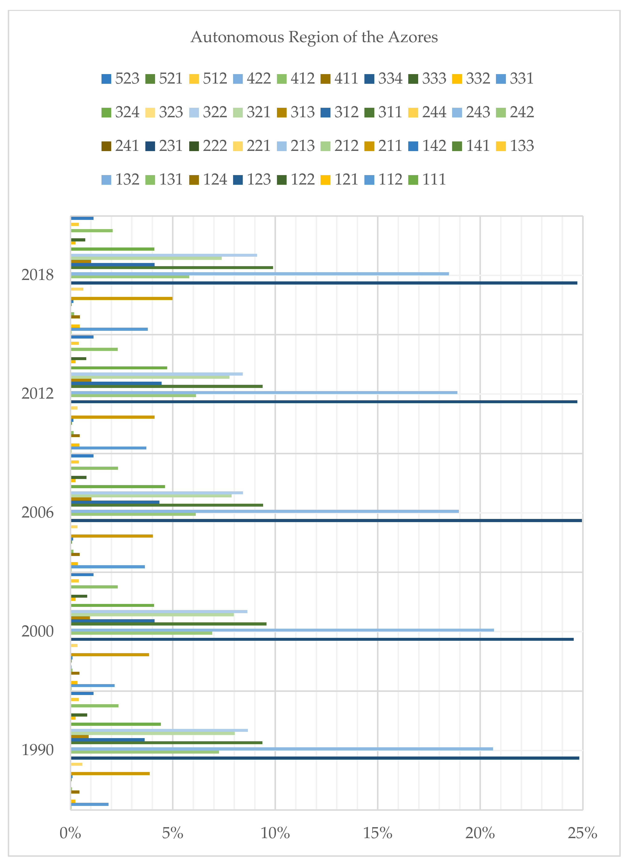
Land-use shows similar patterns in all the Azores’ islands, emphasizing the installation of urban areas next to coastal regions. In fact, some of the obtained results could be explained by the specific geomorphology of each island.

Nevertheless, the predominance of areas related to agricultural and pasture activities, and forests and natural environments between these areas and the islands’ interior is evident.

The territorial areas in which the forest and natural vegetation have greater representativeness are those where there is a protection status, attributed under the Regional Network of Protected Areas or the Natura 2000 Network, contributing to the conservation of biodiversity, strengthening the claim of Azores as a nature destination. Here, the Western Group islands assume a considerable weight, and São Jorge and Pico, with the surface’s occupations by agricultural areas as natural pastures and landscapes, and the forest and natural vegetation of around 60%. The lagoons, usually constituting points of relevant interest for tourist activity, are only represented on three islands: Corvo, São Miguel, and Flores. However, except Graciosa alone, all other islands have inland water bodies of appreciable beauty.

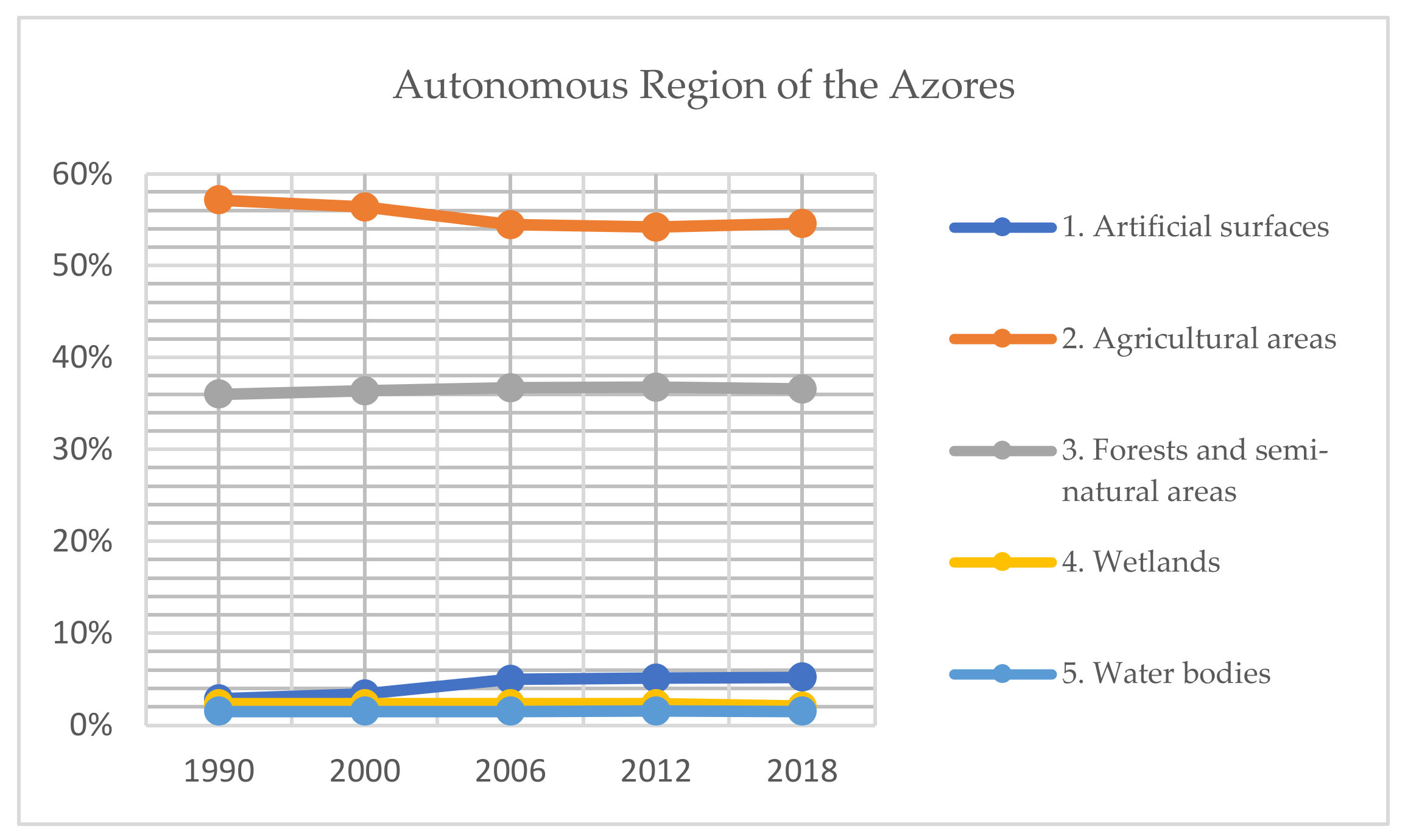
There is a significant increase in urban areas in evolutionary terms, reflecting the urban growth that has been witnessed in recent years. The agricultural and pasture areas have decreased in recent years, considering that in the 1990s, they represented more than 50% of the Azores area. On the other hand, there was an increase in forest areas and natural environments, when in the middle of the 1990s, they represented nearly 30% of the Azores’ territory.

Regarding the artificial occupation of the territory—the urban occupation—about 3.4% of the surface of the territory of the Azores is characterized mainly by discontinuous urban fabric, representing 67% of the total urban fabric of the Azores. Only in the largest island—São Miguel—the continuous urban fabric is predominant, with around 59%. Industry, commerce, general equipment, and infrastructure only represent 0.44% of the Azores’ surface total occupation. The islands with the greatest relative implantation of this economic activity are São Miguel and Terceira—the Azorean economy engines.

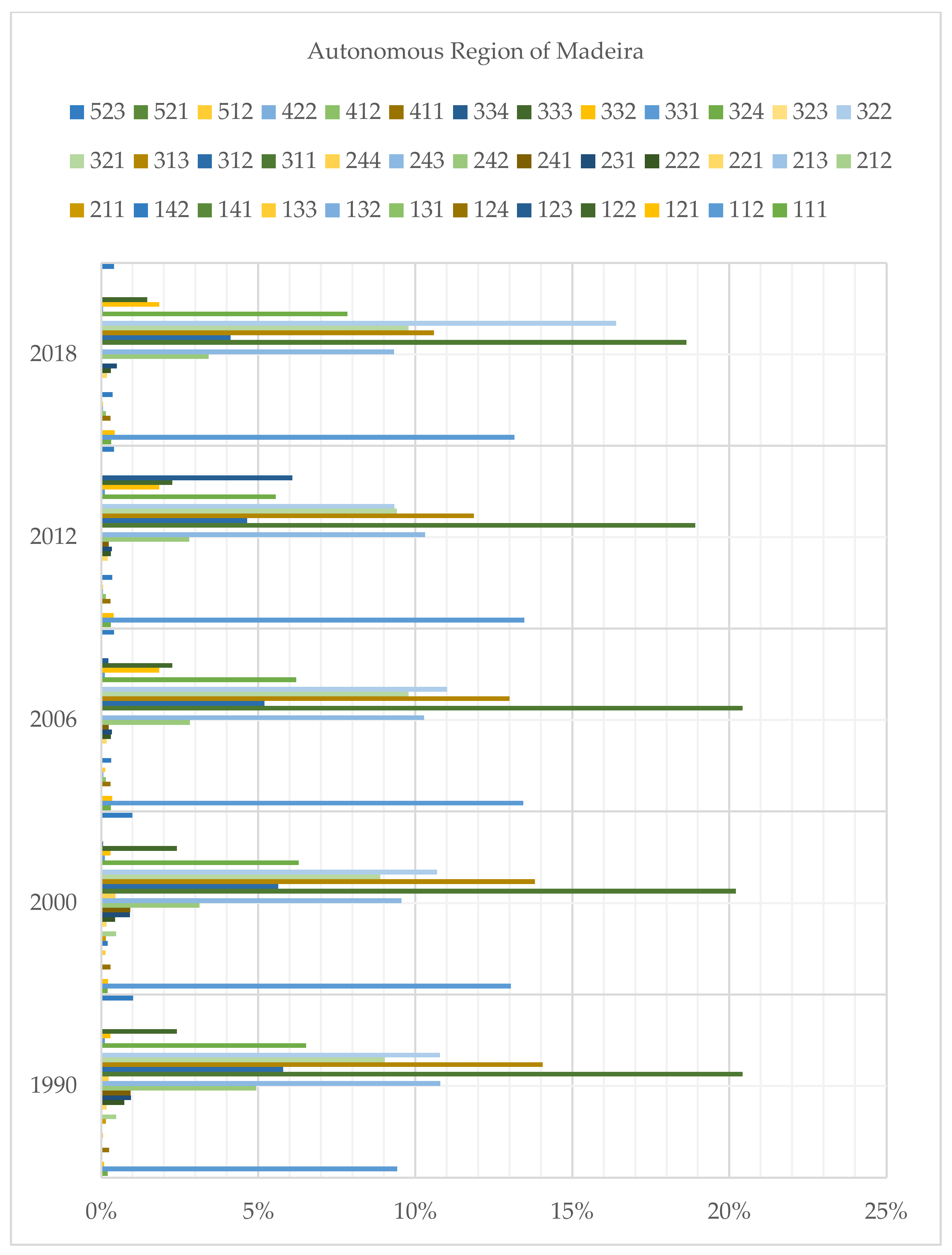
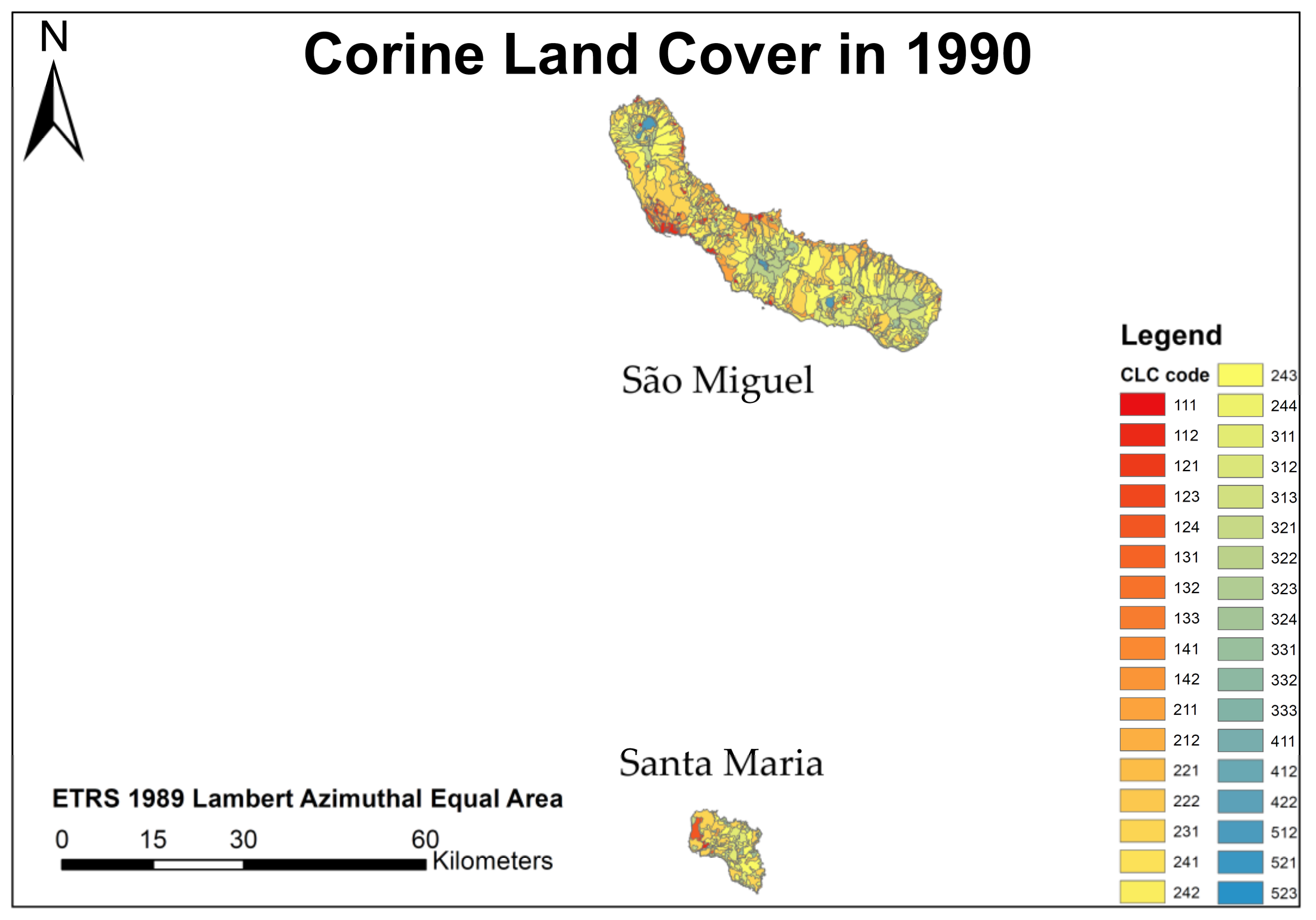
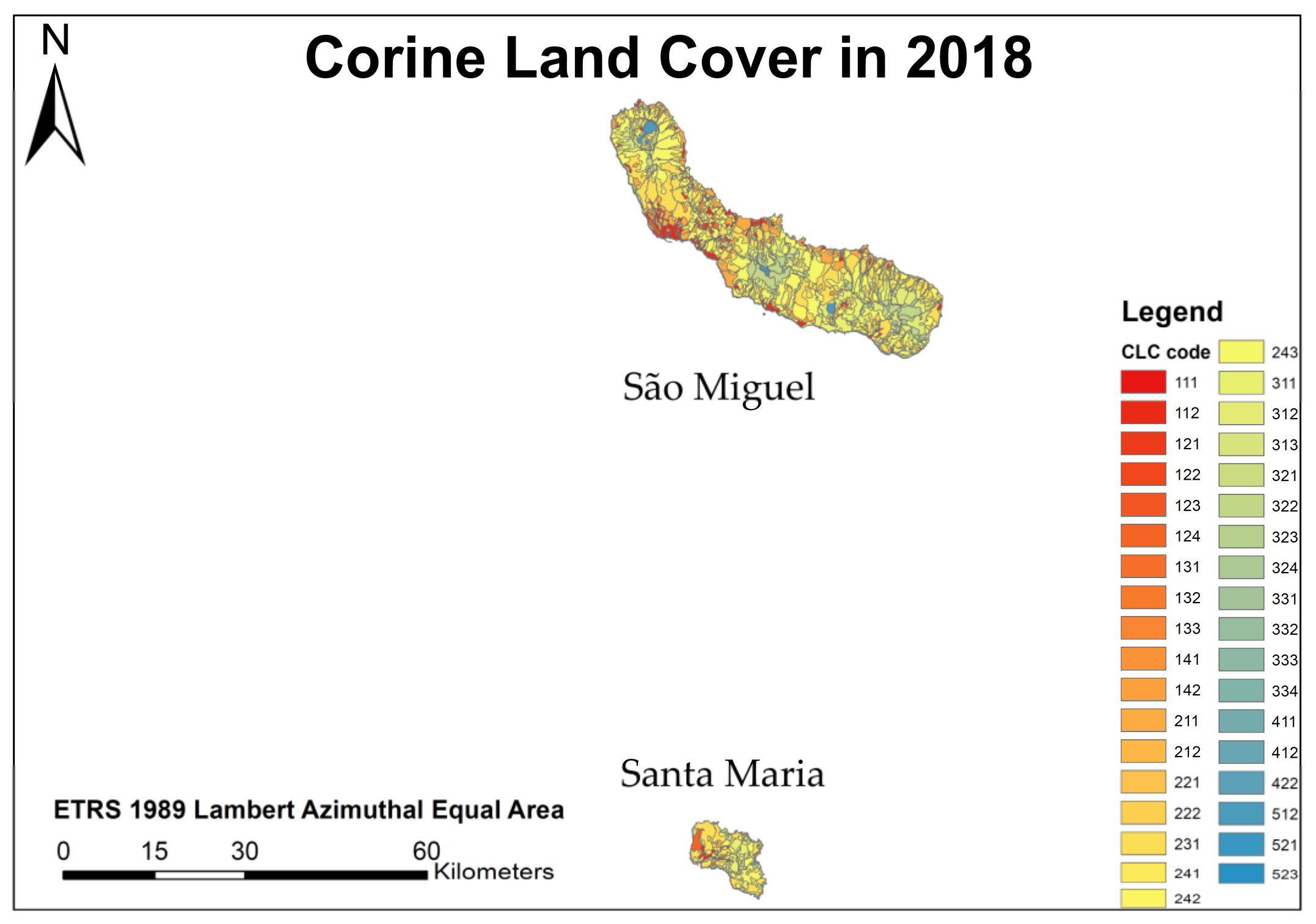
5.2. Madeira Archipelago

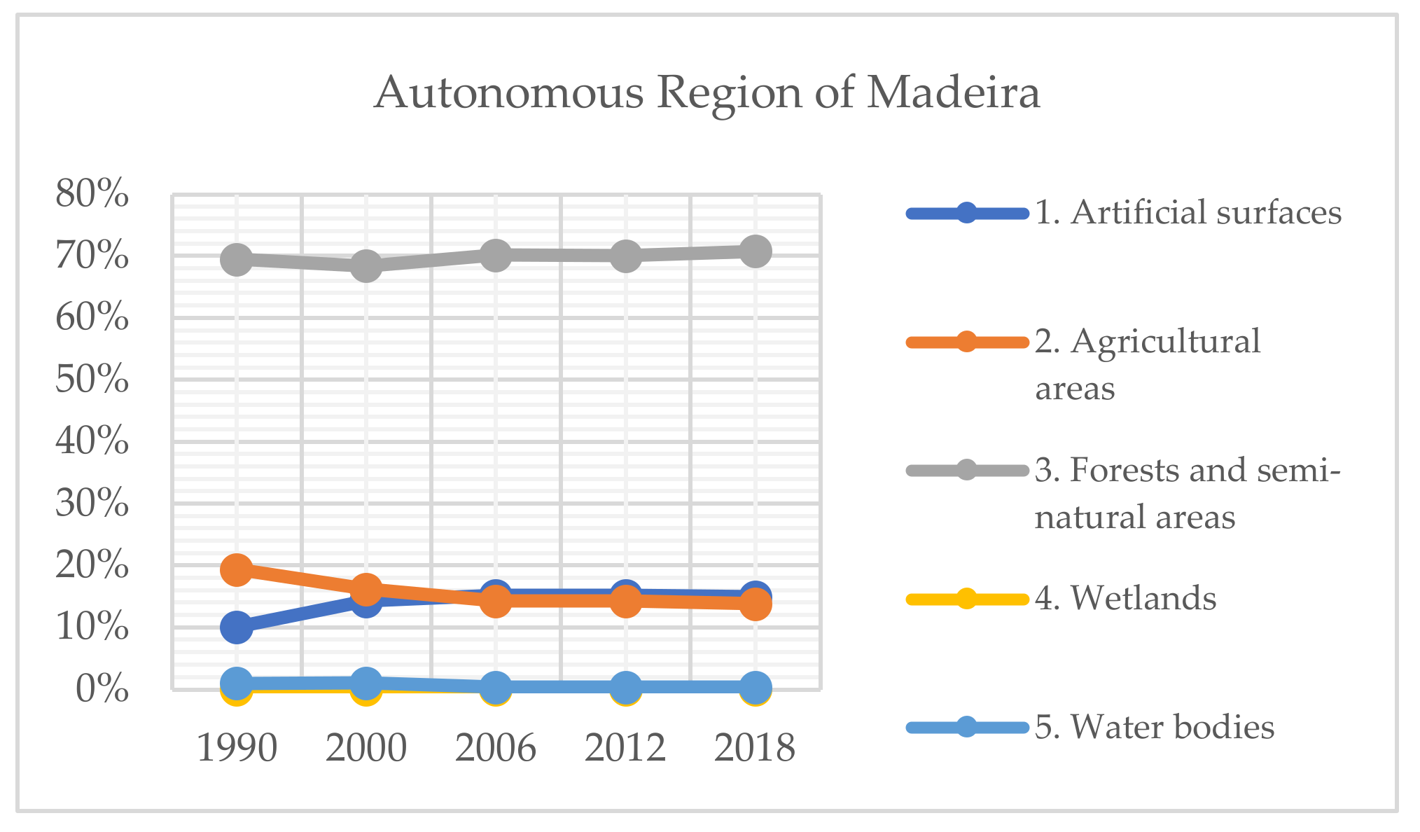
Identifying the different land-uses in the years analyzed in the Madeira archipelago allows for differentiating these land-uses according to their extension, determining which are the most extensive land-uses, and therefore, more hegemonic. Under this criterion, the forest and semi-natural areas constitute the predominant land-use, since it occupies, in all the years analyzed, approximately 70% of the surface of the archipelago, increasing progressively even in all the last years analyzed.

The second most predominant land-use alternates throughout the analyzed years. Between 1990 and 2000 corresponds to agricultural areas. However, between 2006 and 2018, artificial surfaces were the second most predominant land-use, always with percentages of approximately 15%.

In this regard, both agricultural and artificial surfaces between 2012 and 2018 show a downward trend. Likewise, these land-uses are directly related to human activity. Therefore, it could be said that the incidence of humans in the archipelago is becoming less and less impactful in terms of land-uses.

The presence in the archipelago of the remaining land-uses is practically non-existent. Regarding the water bodies, they occupy an area consistently below 1.5%. Besides, they tend to shrink as the years go by. As for the latest use of wetlands, soil practically does not exist. However, both water bodies and wetlands, due to their importance, predominantly environmental, must be monitored in order not to reduce their presence, and thus disappear in years to come.

Regarding the location of the different land-uses on the islands that make up the archipelago, Desert Islands always have the same land-uses; as the name suggests, they are deserted, and the lack of human activity makes the variation in land-use virtually non-existent. The same is not valid on the other islands where other patterns are observed. Thus, on the island of Porto Santo, the artificial surfaces are concentrated in the central region. Besides, these land-uses are usually surrounded by agricultural areas, and forest and semi-natural areas. In this regard, the accumulation of artificial surfaces in the same region could indicate that they are under tourist pressure. As for Madeira’s island, the pattern of location of land-uses is reversed, as artificial surfaces are grouped into outlying coastal areas, mainly in the south and also in the north but to a lesser extent. Additionally, the central part is dominated by land-uses unrelated to human activity. Therefore, this area registers less anthropic pressure.

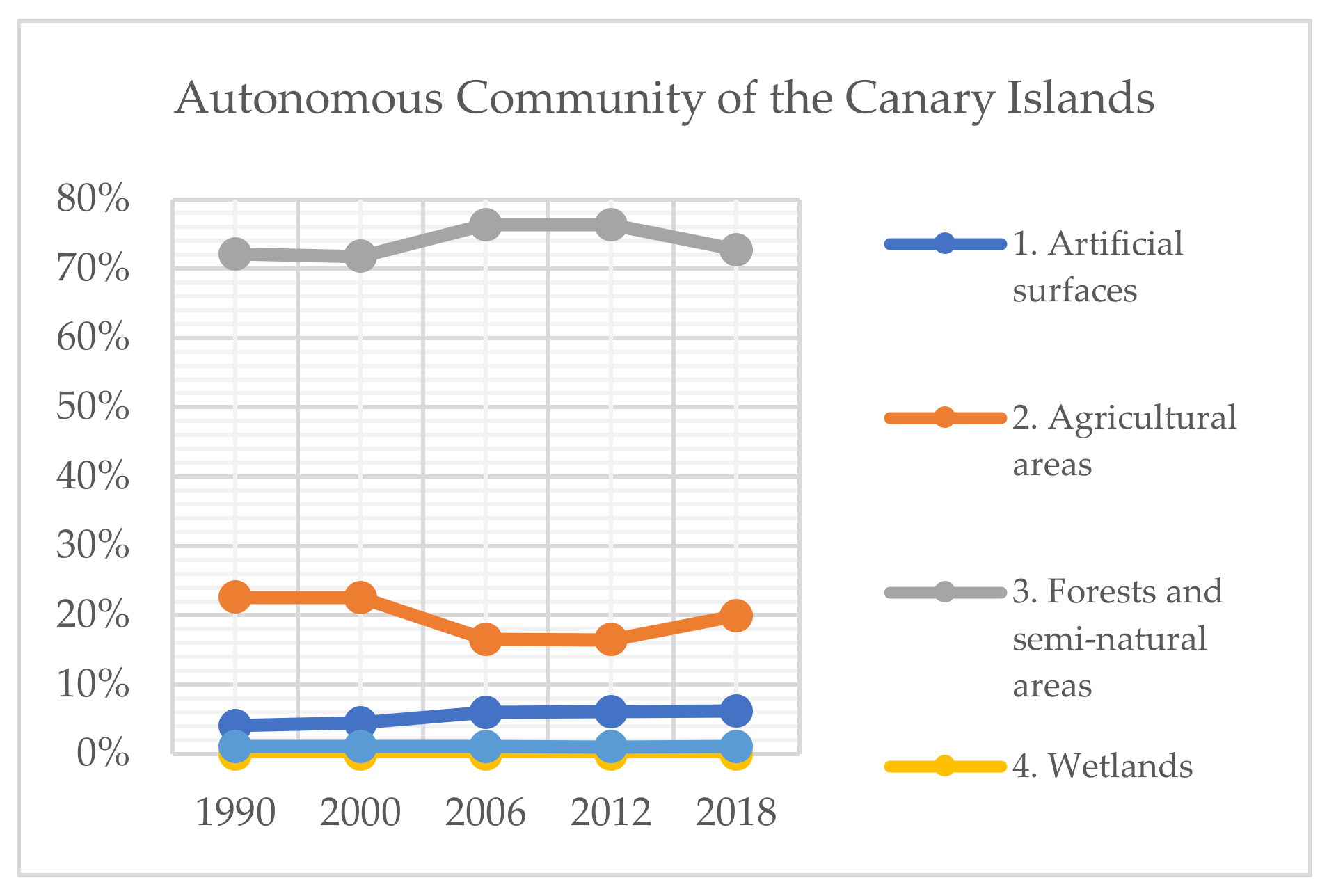
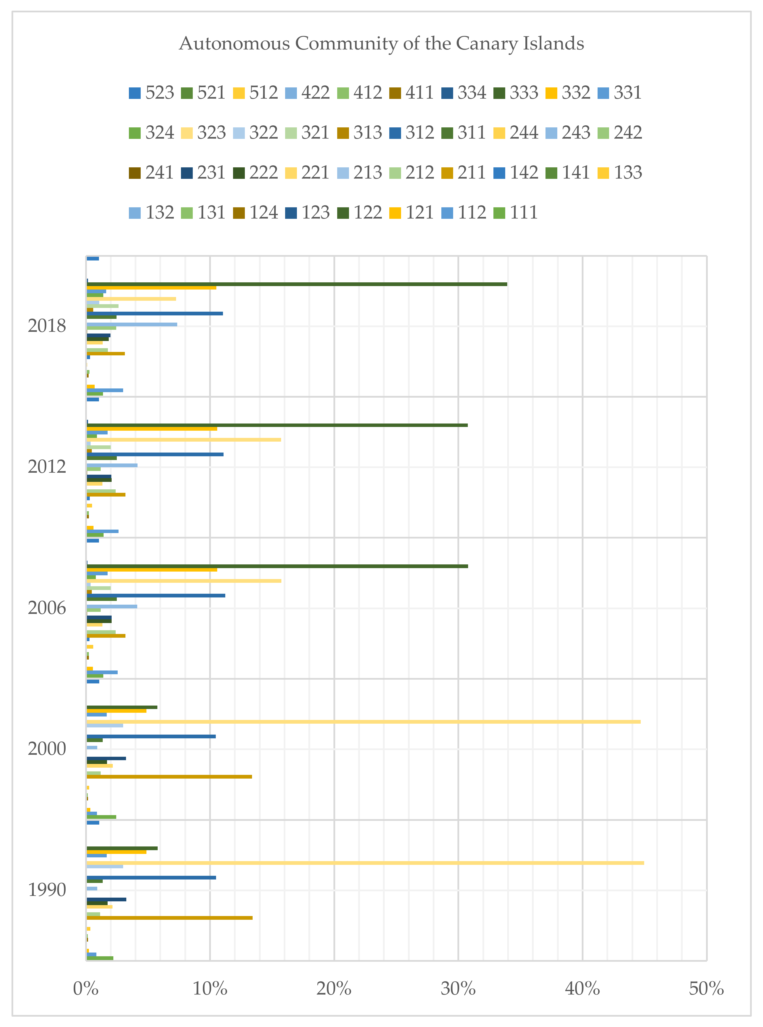
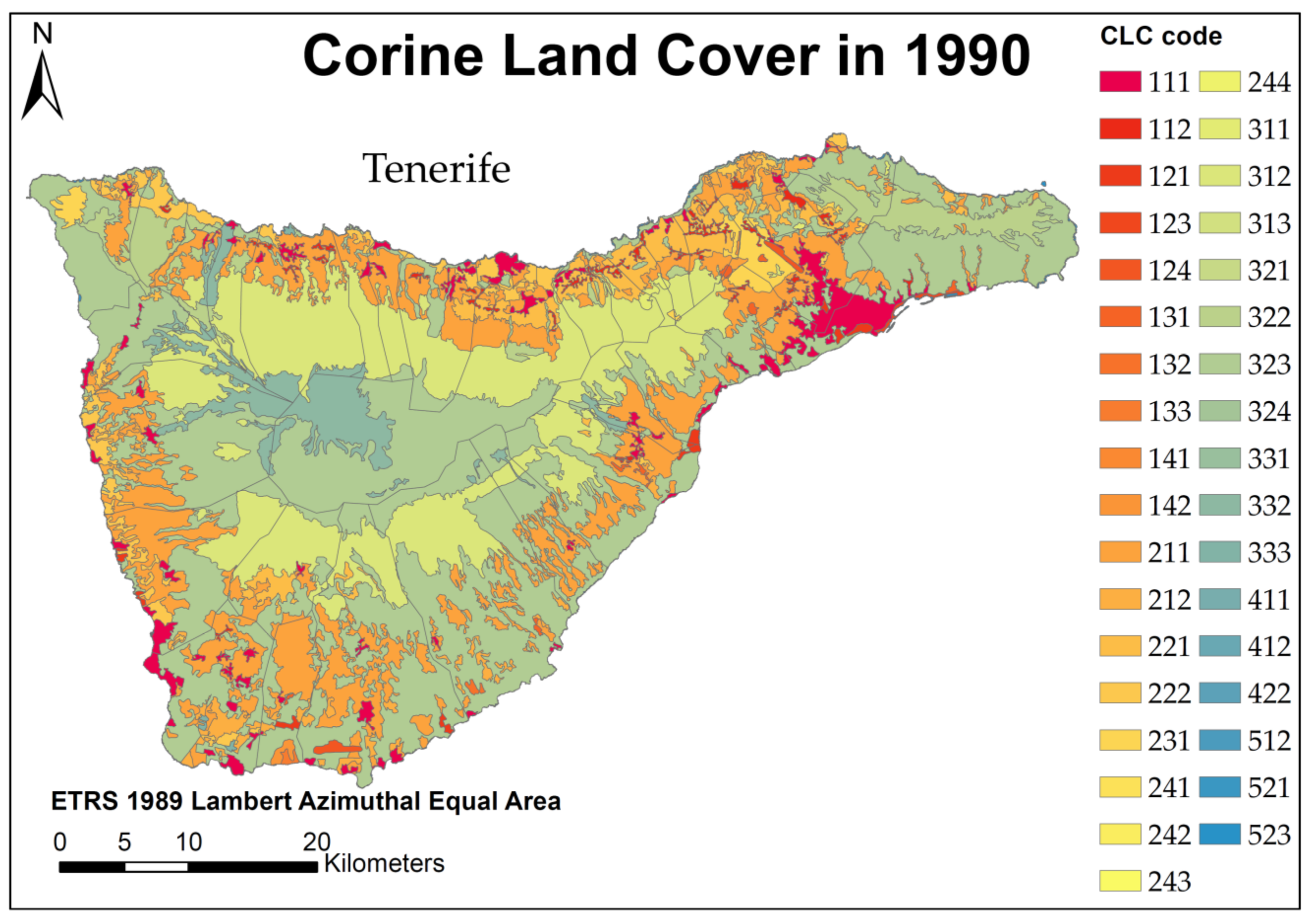
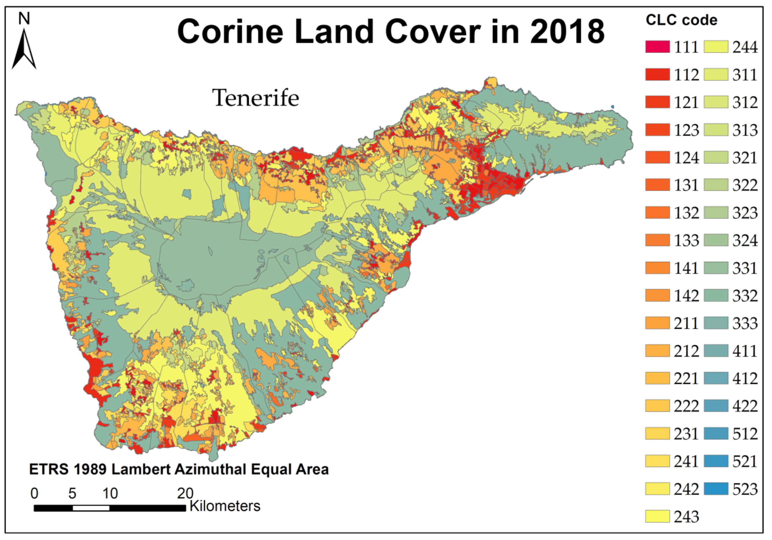
5.3. Canary Archipelago

The predominant land-use corresponds to forests and semi-natural areas, as it occupies approximately three-quarters of the territory. Therefore, this land-use should be used to conserve existing ecosystems in the archipelago. However, over the last three years analyzed (2006, 2012, and 2016), a slight downward trend could continue over the years. However, there is little chance that it will lose its hegemony in the territory analyzed. The second predominant land-use corresponds to agricultural areas, occupying approximately one-fifth of the territory. The third majority use refers to artificial surfaces, occupying approximately 6% of the area analyzed. These last two land-uses are directly related to human activity on the territory, taking into account that their surface area increases slightly over the years analyzed; so, it can be said that the most impactful activity of the human being on the territory analyzed is also increasing slightly. As a result, all activities related to these two land-uses should be monitored. Moreover, water bodies’ existence is residual, and curiously, there are no significant records for wetlands.

As for the location of the various land-uses, more significant variation is observed in areas located on some islands’ peripheries, where there is an increase of artificial surfaces. Among all the islands stand out Tenerife and Gran Canaria, as they are the most populated areas and there is a more intense tourist activity. There is also less anthropic pressure in the internal regions. Therefore, these regions are less exploited by both population pressure and the tourism industry. In fact, in these areas, the use of forests and semi-natural areas predominate, and are spaces that should serve to preserve the eco-systems of the archipelago.

If we analyze this territory more closely and from different perspectives, it is possible to understand the considerable impact of tourism over all the regional economy. In 2017, economic activity represented 85.7% in services (related to tourism), 7.6% in industry and energy, 5.4% in construction, 3.7% in the manufacturing industry, and 1.3% in agriculture and animal breeding and fishing. In the Canary Archipelago, tourism activity obtains a meaningful relevance in numerous contexts due to its economic potential.

In the Canary Archipelago, tourism is a cultural event in which people move freely for a certain period for various reasons, i.e., recreation, rest, culture, or health [53]. According to Santana [54]: “(...) tourism is a complex and dynamic activity in close relationship with society and its nuances—behavior, motivations, values, history, traditions, and beliefs.” In fact, the Canary territory is a tourist destination in the reorientation phase [55]. Contextually, the Canary Islands’ Government is committed to “the renewal, innovation and regeneration” of the tourist area, always having northern tourism of higher quality [56]. Additionally, tourism planning inevitably includes planning both in terms of tourism and spatial planning [37]. Therefore, it is common to have land-use policies, namely legislation on the territory’s division into fields varying from environmental protection categories to control tourism development spaces [57]. Nonetheless, spatial planning usually results in the “post” when several destinations are previously openly overloaded or threatened [58].

5.4. General Conclusions

The remote islands face many challenges today as land-use changed from 1990 to 2018, along with the increase in the number of visitors, when the demand for living space increased and the resource capacities were limited. As we have seen, it has not been possible to maintain the islands’ situation as it was before, and change will continue to be made. What is essential is that the living environment and the island areas’ unique character should be preserved and protected; the priorities must be defined, and management strategies established which are significant for the well-being of these highly valued areas. Forestry, as the traditional land-use and predominant land-use in island areas, especially in Madeira Archipelago and Canary Islands (over the last three years analyzed (2006, 2012, and 2016), a slight downward trend) should support sustainable forestry as an appropriate form of land-use. With responsible management, the natural resources of island areas can be used for a long time [61,62,63,64,65]. Degradation of water quantity and quality cannot be overlooked, particularly on some small islands where groundwater conditions have completely changed. It is possible to identify a notable increase in the artificial surfaces (Code 1) in the Azores and Canary islands during the study period. In addition to recognizing that agricultural land is traditional, and agriculture is a valuable activity, it is necessary to encourage agricultural management practices that are compatible with the sustainable development of islands area [65,66,67,68]. As examples of these practices, it is possible to name some as: use of renewable energy sources; integrated pest management; hydroponics and aquaponics; crop rotation; polyculture farming; permaculture; avoiding soil erosion; crop diversity; among several others. According to ESPON Program for the Develpment of the Islands [68]: “Due to the relatively small land masses and isolation, islands are typically land-resource constrained. This limits living space, space for infrastructure, waste disposal, agricultural production, industrial development, water resource availability, among several others. Additionally, it results in very vulnerable ecosystems with high endemism.” Thus, pressures resulting from anthropogenic factors can have more critical consequences on insular environments, invaliding their capability to supply goods and services, and sustain life.

Detailed analysis metrics have been presented throughout this work as a helpful instrument in the analysis, monitoring, and monitoring of changes in land-uses, through different levels of analysis until their application as a comparison tool in different temporal situations.

In this sense, patch analysis shows that there is greater fragmentation in each of the regions analyzed. In addition, the class analysis makes it possible to establish that there has been no increase in land-uses in the Azores Autonomous Region. On the contrary, in the Autonomous Region of Madeira and the Autonomous Community of the Canary Islands, diversity in land-uses was increased. It could therefore be said that in the latter two regions, anthropic activity has been greater. More compact shapes are generally observed in the latter two regions. In addition, landscape metrics make it possible to state that the Madeira Autonomous Region, despite being the smallest in the extension of the areas analyzed, is the one with the greatest diversity, although in decline in the years analyzed. On the contrary, there is less diversity in the Autonomous Community of the Canary Islands despite being the most extensively analyzed region.

5.5. Study Limitations and Prospective Research Lines

The limitations of this study are directly related to the technical limitations of CLC. In this regard, if we consider the three analysis components that we can deal with a GIS, it is possible to describe each of them.

As for the spatial component, the geometric accuracy has been going down over the years, analyzed from 50 m to be below 10 m. While it has improved considerably, this could have been slightly better in the years leading up to 2018, and it would be optimal for it to be improved over the years to come. Moreover, while it is true that the minimum mapping unit and minimum mapping width have always been the same over the years, 25 hectares and 100 m respectively, it would have been optimal to have lower minimum mapping units. However, the minimum mapping unit is considered appropriate for the extent of the analyzed terrain and the scale of data processing geometric accuracy. Regarding the thematic component, the accuracy in identifying the various land-uses has always been equal to or greater than 85%. Therefore, although there is a slight range of improvement, this accuracy has always been high.

Concerning the landscape metrics recorded, a more specific analysis focused on more specific objectives would be desirable to determine the evolution of some of the land-uses analyzed.

Finally, concerning the temporary component, the last update to land-uses occurred in 2018. It would therefore be optimal if there were more up-to-date land-use data. Besides, note that the products offered by CLC are of high quality and rigorous. Furthermore, these products are open and cover a large area of territory.