
Tree Height Growth Modelling Using LiDAR-Derived Topography Information


Department of Forestry and Renewable Forest Resources, Biotechnical Faculty, University of Ljubljana, Večna Pot 83, 1000 Ljubljana, Slovenia
*
Author to whom correspondence should be addressed.
ISPRS Int. J. Geo-Inf. 2021, 10(6), 419; https://0-doi-org.brum.beds.ac.uk/10.3390/ijgi10060419
Submission received: 23 April 2021
/
Revised: 11 June 2021
/
Accepted: 18 June 2021
/
Published: 19 June 2021
(This article belongs to the Special Issue The Use of Geo-Spatial Tools in Forestry)
Abstract
:The concepts of ecotopes and forest sites are used to describe the correlative complexes defined by landform, vegetation structure, forest stand characteristics and the relationship between soil and physiography. Physically heterogeneous landscapes such as karst, which is characterized by abundant sinkholes and outcrops, exhibit diverse microtopography. Understanding the variation in the growth of trees in a heterogeneous topography is important for sustainable forest management. An R script for detailed stem analysis was used to reconstruct the height growth histories of individual trees (steam analysis). The results of this study reveal that the topographic factors influencing the height growth of silver fir trees can be detected within forest stands. Using topography modelling, we classified silver fir trees into groups with significant differences in height growth. This study provides a sound basis for the comparison of forest site differences and may be useful in the calibration of models for various tree species.
1. Introduction
The ecotope as a pure land unit of the lowest rank was presented as a central concept in landscape ecology [1,2,3,4]. The ecotope is recognized as an ecologically relatively homogeneous, spatially explicit, functional landscape unit with at least one homogeneous land attribute, and only small variations in other attributes such that gradients within an ecotope cannot be distinguished. In forestry, the term ‘site’ is similarly defined as a geographical location that is homogeneous in its physical environment with respect to climate, topography, soil and vegetation [5,6,7]. Both concepts describe correlative complexes defined by landform, the structure of vegetation forming various cover types, the characteristics of vegetation in the forest stands and the relationship between soil and physiography [2,5]. Naveh [8] proposed that the boundaries of ecotopes could be established pragmatically, based on the subject and the objectives of a particular study, while remaining concretely placed within a certain space and time as actual ecosystems [1].
Similar concepts have been adopted for the purpose of analyzing and mapping ecological units at landscape and regional levels. Species assemblage has been used as a categorical variable at the regional scale and in landscape research, based on the assumption that the distribution or pattern of vegetation is influenced by environmental factors [9,10,11]. Over the past several decades, the development of land classifications has been supported by satellite multispectral (MS) imagery and terrain data that can be used to map land classes over large areas. Rasti et al. [12] provided a technical overview of the state-of-the-art techniques of feature extraction approaches for hyperspectral images. Hyperspectral imaging (HSI) can acquire richer spectral information by sampling the reflective portion of an electromagnetic spectrum, covering a range from the visible to the short-wave infrared region and also the emissive properties of objects in the range of the mid-wave and long-wave infrared regions. HSI technology enables the detection and a high discrimination ability between spectrally similar classes, but its coverage from space is much narrower than the MS ones. In order to obtain a more accurate abundance estimation, Hong et al. [13] proposed a new method for HS image analysis that models the main spectral variability and variability caused by environmental conditions, the instrumental configurations and the material nonlinear mixing effects separately. To exploit the rich spectral information contained in HS images, they are developing new methods and fusion strategies that will reduce the limitations due to high storage and computational cost [14].
Topographic variables are often used as surrogates or predictors for the environmental gradients that affect species, vegetation or ecosystem class distribution [9,15,16,17]. Pfeffer et al. [18] showed that, despite the impact of natural and artificial disturbances on the spatial pattern of alpine vegetation, topography was still an important environmental factor. Dirnboeck et al. [19] stressed the importance of matching topographic data to the scale at which the spatial patterns displayed by mapping units are influenced by biophysical constraints. In calcareous alpine environments, the coarse resolution of the digital elevation model (DEM 50 m) misses most of the microscale variations in site conditions.
Physically heterogeneous landscapes, such as karst landforms developed in limestone and dolomite bedrock, e.g., dolines or sinkholes, where steep slopes alternate with depressions, display special topographical, hydrological and subterranean properties [20]. Despite a relatively homogeneous parent material, karst relief is characterized by furrows, grykes and different types and combinations of sinkholes. The microforms of a terrain are assumed to be more important factors in soil formation and vegetation patterns than the macro-scale landforms of the surface. In high karst areas, luvisols are typically present at the bottom of sinkholes as a result of the flow and rinsing of water and sediment [21] from the edges of sinkholes and ridges, where more shallow soil types are prevalent, especially leptosols and shallow cambisols. Significant differences in vegetation diversity and composition occur inside and outside the sinkholes, which indicates their presence has important ecological impacts [22]. Within forest ecotopes, the soils of steep and rocky surfaces are often shallow and less developed and contain a higher amount of organic matter [23,24]. Consequently, growth conditions and forest vegetation can change rapidly, even within very short distances [25]. Based on vegetation surveys and soil analyses of diverse microtopographic site conditions, it is difficult to determine the boundaries between the smallest homogeneous units and adapt them to research or forest management problems [24].
As with ecotopes and their gradient assessments, forest sites can be used to represent the environmental factors that impact the growth and yield of the tree species in a given area. Yield tables and site index concepts were used to estimate future forest stand development and to compare various site conditions within forests [5,26,27]. In forestry, parsimonious models have been established based on assumptions of tree height at certain ages. However, the assumptions for estimating site index were restrictive, as forest stands were assumed to be even-aged, monospecific, fully stocked and free of disturbance [28]. Curt et al. [29] have shown that correlations among physiography, climatic indices, soil properties and plant associations are useful site index surrogates. In evaluating techniques for modelling forest site productivity in different ecoregions, site quality has been explained as resulting from different environmental variables [30], with the validity of the empirical models being restricted to the spatial scale for which they were developed. As shown by [31], site index models for small areas require a higher resolution to accurately represent the short-distance variability as well as the relevant environmental patterns of subregions.
The main obstacle to such an indirect concept of site index estimation in karst terrain is the high diversity of landforms, which can affect site conditions and produce variable soil conditions within forest ecotopes. In high karst areas, diverse growth and stand conditions are present on small scales, raising the key challenge of determining how to separate environmental gradients to define the differences between sites. However, spatial models can be adopted to determine the differences in gradients within tangible forest ecotopes. Many studies have demonstrated the ability of an airborne LiDAR system to penetrate dense forest canopies and reveal the underlying ground topography in karst landscapes [22,32,33]. The LiDAR system was able to detect a variety of differences in ground elevation and karst topography based on a generated high-resolution DEM with a cell size of 1 m.
The objectives of this work were to assess the influence of topography on the tree growth in karst terrain. The following research questions were addressed: (i) Are the growing conditions of individual trees influenced by landforms and topographic factors? (ii) Is a LiDAR-derived DEM with a 1-m resolution appropriate to detect terrain-related gradients and microsite conditions? (iii) Is the difference in tree growth on different landforms large enough to be indicative for the forest management and silvicultural operations?
To analyze the effect of topography on tree growth, we selected uneven-aged forest stands with diverse microtopographic site conditions in the high karst area of the Leskova dolina Forest Management Unit (FMU). We examined the applicability of a DEM-based spatial model of landforms and topographic factors for forest management and silvicultural treatment. The present study was motivated by the need for a spatial model that can be used to compare site or ecotope gradients under field conditions with a special focus on karst terrain.
2. Materials and Methods
2.1. Study Area
This study was conducted in southwestern Slovenia (Figure 1) in mixed, uneven-aged forests. The Dinaric silver fir—European beech forests of high karst areas ranging in elevation from 500 to 1200 m above sea level—form one of the largest forest complexes in Central Europe. In the western and central Dinaric Mountains, uneven-aged forest management has been predominant for over a hundred years [34].
As the forests of high karst areas were not as easily accessible, they have been subject to lesser changes than forests elsewhere in Europe. The species composition of these forests still predominantly consists of silver fir (Abies alba Mill.), European beech (Fagus sylvatica L.) and Norway spruce (Picea abies L.). In the study area of the Leskova dolina, the predominant old-growth forest species at the beginning of the 19th century were European beech and silver fir, with abundant silver fir regeneration. It is estimated that two-thirds of all currently living fir trees in the study area regenerated between the beginning and the middle of the 19th century [37]. However, a period of unsuppressed growth began at the end of the 19th century, when foresters initiated cutting with greater intensity and favored silver fir due to its greater economic importance compared to European beech. Following [38] the vegetation classification commonly used in Europe to characterize forest associations, Omphalodo-Fagetum typicum, Omphalodo-Fagetum mercurialetosum and Omphalodo-Fagetum homogynetosum represent prevalent sub-associations, defined as the lowest rank of the phytocoenological classification in the research area.
2.2. Experimental Design
2.2.1. Plot Establishment
A detailed research site (19.75 ha) was selected in the Forest Management Unit, Leskova dolina (Figure 1), based on the following criteria: (i) Silver fir should be the dominant tree species of the site. (ii) Selected fully stocked mature stands should be preserved and free of disturbance. A research site lying between 820 and 871 m above sea level was selected in one of the forest compartments (No. 34) after reviewing the data from forest management plans for the period from 1890 to 2004, also used and analyzed in several studies in Leskova dolina [37,39].
Sixty-five circular sampling plots with a surface area of 500 m2 were established in a 50 × 50 m sampling grid in the study area. In each plot, the diameter at breast height (dbh over bark) of each tree exceeding 10 cm dbh was measured. The study area includes five tree species. The prevailing tree species was fir, accounting for 85.4% of the growing stock in the plots. The average growing stock measured 642.4 ± 32.2 m3/ha. The average number of trees per hectare was 367 ± 24, including 207 ± 14 fir trees and 145 ± 23 beech trees, with the latter accounting for 10.5% of the growing stock. The remainder of the growing stock was made up of spruce (1.9%), sycamore (2.0%) and elm (0.2%).
As the average height of dominant and codominant trees (top height) is considered to be an estimator for site quality assessment and proposed in growth modelling [27], we selected one of the dominant fir trees from each of the plots for stem analyses. Dominant trees were used for the stem analysis because the height growth of the largest trees is assumed to be independent of silvicultural treatment and of changes in stand density [40]. Typically, top height is estimated based on the average height of the 100 thickest (largest diameter at breast height) trees per hectare. In operational forest inventories or in growth and yield studies based on sample plot data [41,42,43], it is common practice to use the corresponding proportion of trees according to the plot area, e.g., the mean height of the five largest trees in 0.05 ha sampling plots. Our sample plots were used to determine several characteristics of forest stands, the conventional method of estimating top height was adopted for selecting a subsample from dominant silver fir trees. From these, we identified the 5 thickest trees, and we selected the third thickest for stem analysis to reconstruct the height growth of dominant silver fir trees on different landforms. In forest inventories, mean heights and mean ages are usually measured for one or two representative median trees [44]. On sample plots in the study area, we selected 65 dominant silver fir trees representing the average dbh, 59.0 ± 1.6 cm, and mean height, 34.0 ± 0.8 m.
2.2.2. Airborne Laser Scanning
Scanning was carried out by a private company using a Eurocopter EC 120B helicopter flying between 400 and 600 m above the land surface and a full-waveform laser scanner (Riegl LM5600) with a relative horizontal accuracy of 10 cm, a relative vertical accuracy of 3 cm and a remote laser impulse frequency of 180 kHz. To define an accurate trajectory and helicopter orientation path, a Novatel OEV/OEM4 GPS receiver and an optical INS IMU-IIe were used to record GPS measurements with a frequency of 10 Hz. The laser point density measured 30 points/m2, and the laser footprint was 30 cm. The scanning was carried out in October 2009.
2.3. Laboratory Work
2.3.1. Detailed Stem Analysis
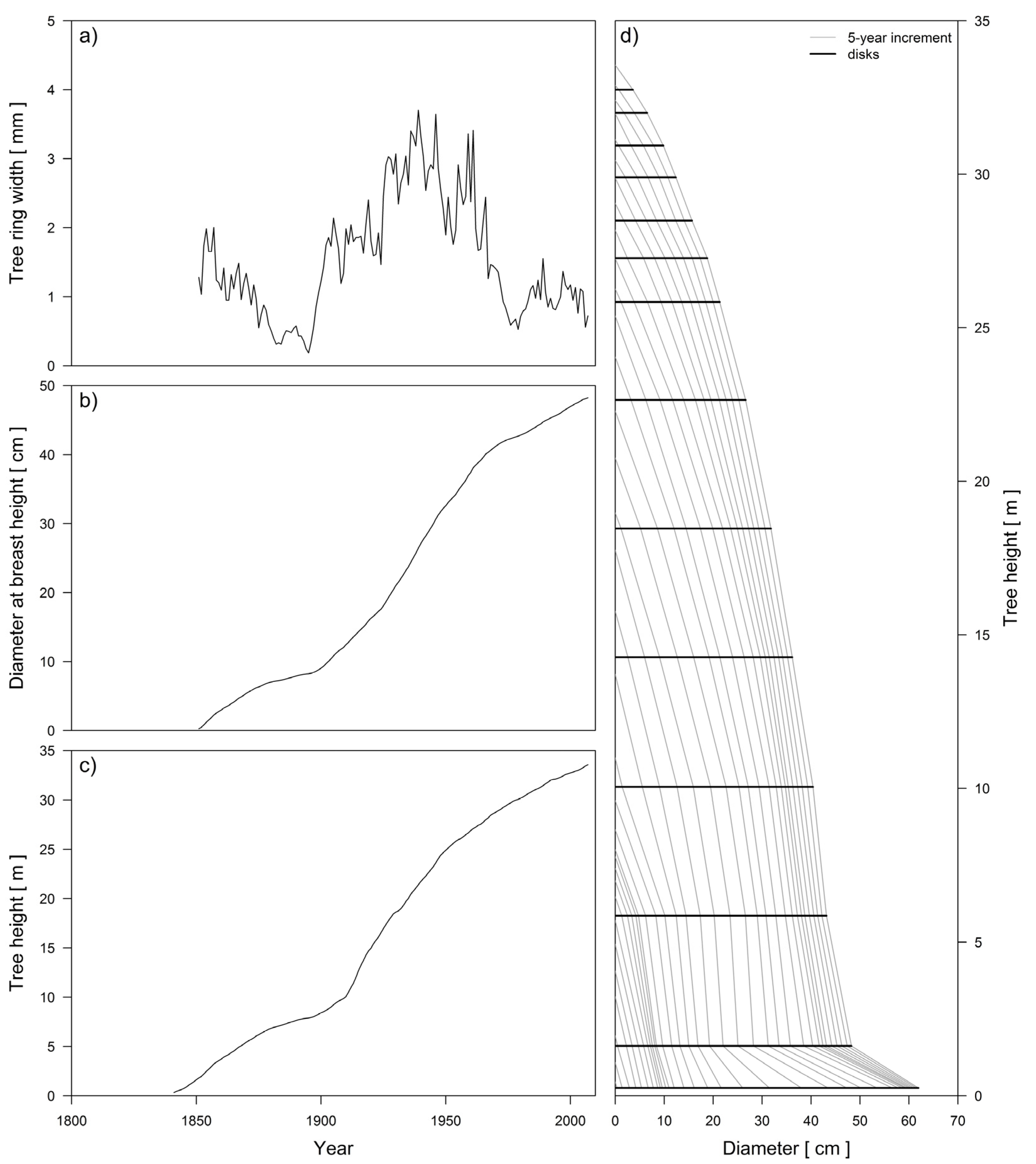
Disks from the felled fir trees were cut at the tree stump, at breast height and then every 4 m until a diameter of 30 cm was reached. The top of the stem (diameter < 30 cm) was cut in 1-m-long sections. Thus, we acquired 992 stem disks, and out of the middle of each, a rectangular block was cut. The widths of the annual rings in each block were measured in two directions with 0.01 mm accuracy using ATRICS [45] and WinDendro [46] software. Each series of annual ring widths was additionally examined with the PAST-4 computer program [47], and the arithmetic means were calculated for both series of annual ring widths. Detailed stem analysis was performed using software written specifically for our study in the R programming language [48]. This software enables the past height growth history of a tree stem to be reconstructed (Figure 2).
We used the correction proposed by Carmean [49] to estimate the height growth of each analyzed tree. This method assumes that the annual height growth within a given stem section is constant and that the crosscut was made in the middle of a given year’s height growth. The height growth increments were calculated for the last 100 years.
When comparing the height growth of dominant trees from the uneven-aged forest stands, the period of suppressed growth for silver fir as a shade-tolerant tree species as well as age differences among the trees were estimated. Suppressed growth in youth was considered a consequence of natural regeneration under shelter. Silver fir ages ranged between 132 and 209 years, with an estimated mean age of 178.5 ± 4.2 years. Consequently, the ages of these trees are not comparable to the ages of trees of the same height growing in even-aged stands after clearcutting [50]. Based on the stem and dendrochronological analysis, we concluded that the trees showed no sign of suppressed growth after they reached a height of 14 m. To compare the height growth increments of the dominant silver firs, we determined their average height growth increment between 14 and 24 m.
2.3.2. Digital Elevation Model Processing
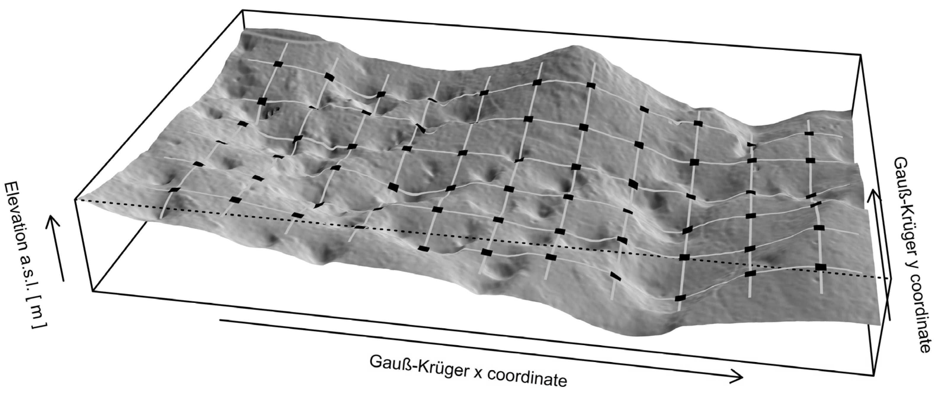
The processing of LiDAR data was performed using Microstation v2004 (Bentley) with Terrasolid software packages. For the classification of points, a Terrasolid algorithm was used. This algorithm enables the development of a surface model based on the detected ground reflections [51] to successfully remove the forest from scans without losing topographic survey details. From the survey points, a triangular network using Delaunay triangulation was created in the ArcGIS environment and the points were transformed into a raster format with a basic cell size of 1 × 1 m (Figure 3). Kobal et al. [22] provide a detailed analysis of LiDAR data processing in the FMU, Leskova dolina.
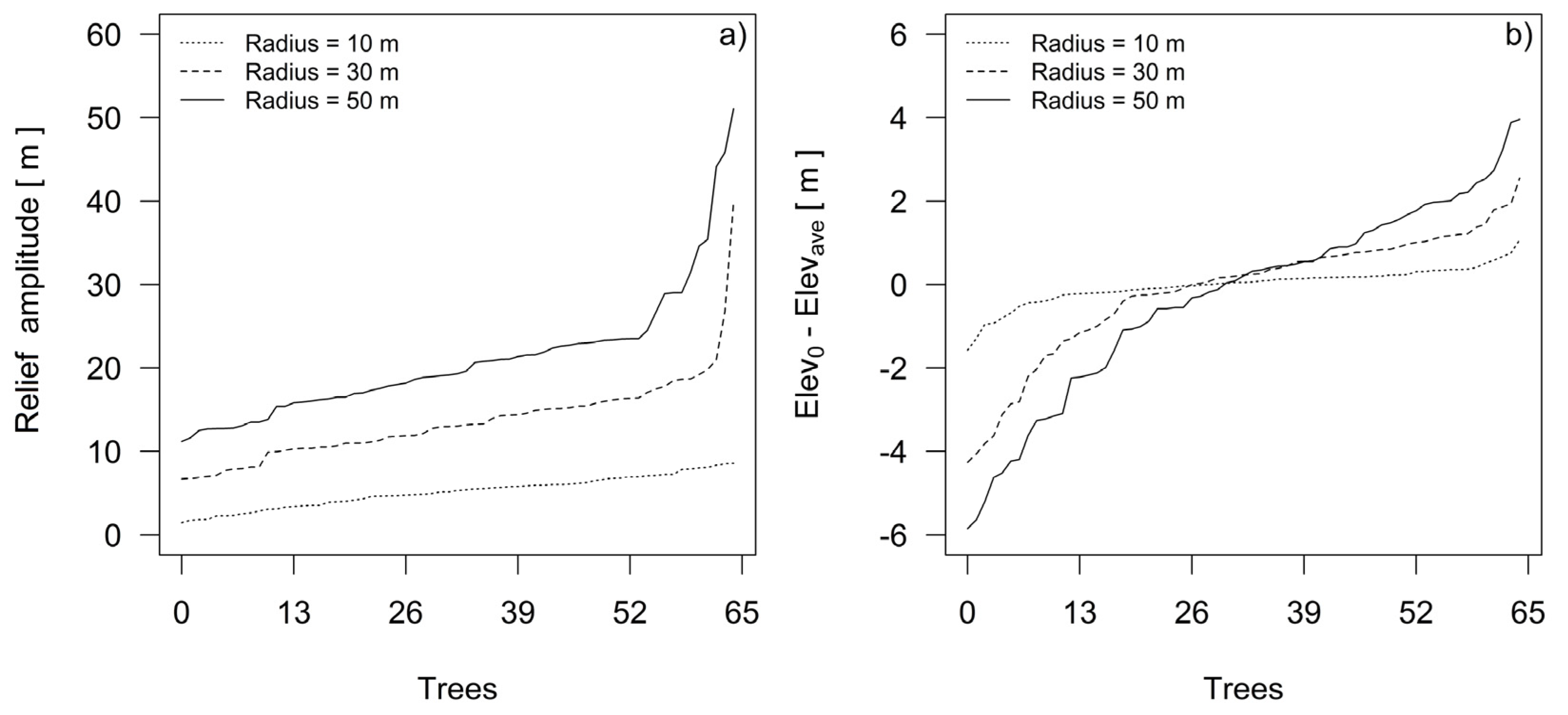
Using the DEM, we estimated the relief amplitudes for every plot’s dominant fir tree, and we calculated the differences between the elevations at the tree base point positions and at the average height positions in their growth sites. We measured the relief amplitude and elevation differences as functions of the radii centered at the stem positions of each dominant silver fir tree in the sample (Figure 4). Since the trees were cut down for stem and dendrochronological analysis, we were able to measure the position of their stumps using a Leica CS10 GNSS receiver. To estimate the relief amplitude defining the sites of individual trees, we calculated the maximum difference, or range, of elevations in the cells of the circle. The difference between the elevation at the tree base point position in the relief and the average elevation of all of the surrounding cells was estimated in the ArcGIS environment using buffers ranging in radius from 10 to 50 m, which was the distance between the centers of field sampling plots on the systematic sampling grid.
For most of the sampled silver fir trees, differences in relief amplitudes were estimated at radii greater than 30 m (Figure 4a). The differences between elevations at the base point position of the trees and the average elevation differences on their growth sites (Figure 4b) show that the sample includes trees that grew on ridges, with average elevation differences of up to 4 m, and trees in sinkholes, which we conclude on the basis of average elevation differences of −6 m. In the next step, a clearer classification for relief forms was obtained by estimating topographic position indices.
The relief was evaluated by surface topographic categories classified by slope position, i.e., a sinkhole, a slope or a ridge. To this end, we used an algorithm developed by Weiss [52], which uses a moving window [53]. First, we calculated a Topographic Position Index (TPI). For each cell in the matrix (a digital model of a DEM relief), the elevation difference between the observed cell and the average elevation of its adjacent cells was calculated. If the average elevation of the adjacent cells was higher, the TPI value was negative (TPI < 0). If the elevations of the observed cell and the adjacent cells were similar, the TPI value was approximately 0 (TPI ≈ 0). If the elevations of the adjacent cells were lower, the TPI value was positive (TPI > 0). Second, the surface topographic category was determined using the TPI. For this calculation, the slope and the standard deviation (SD) of the elevation within the moving window were considered in addition to the TPI.
The surface topographic categories were determined using the R programming language [48]. The criteria for classifying the surface topographic categories were the following:
| Ridge category | TPI > 0.5 × SD |
| Middle slope category | −0.5 × SD < TPI < 0.5 × SD |
| Sinkhole category | TPI ≤ −0.5 × SD |
Since the topographic position is an inherently scale-dependent phenomenon [52,53], the main contribution of our work is to propose a novel approach to determine the scale of topographic categories and landforms that can be used to compare site or ecotope gradients and may offer insight into the spatial variability in site conditions. To assess forest site differences and gradients in site conditions, the scale was determined and verified on the basis of statistical analysis related to tree height growth. By detecting terrain-related gradients and landforms, we were able to identify three groups of dominant silver fir trees.
2.4. Statistical Analysis and Model Selection
Figure 5 presents a flowchart of modelling the scale of topographic categories and mapping three categories of landforms using LiDAR DEM. A one-way ANCOVA was used to assess the interaction of the silver fir dbh with landform categories over the height of the dominant trees. To estimate the growing conditions on different landforms, we compare two models that express the dominant height as a function of tree diameter without considering landform categories (Equation (1)) and consider three categories of landforms as classified predictors (Equation (2)), controlling for the effect of silver fir dbh (continuous covariate), which is considered a ‘nuisance’ parameter. The following logarithmic function was chosen to fit height curves, among a variety of functions that have been proposed and applied in practice [27]:
hi = b0 + b1 × ln(dbhi) + ei
hi = b0 × landform + b1 × ln(dbhi) + ei
The iterative process (Figure 5) to determine the optimal moving window size and TPI scale started from a scale of 3 m (3 × 3 moving window size) and stopped at a scale of 200 m, according to previously estimated relief amplitudes in the neighborhood of sampled trees (Figure 4).
The optimal moving window size was determined by varying it from 3 × 3 to 200 × 200 pixels and seeing their effects in the adjusted R2 of Equation (2). The optimal moving window was defined as the one related to the highest adjusted R2. Models were compared using partial F-tests, Akaike’s Information Criterion (AIC) and adjusted R2.
A one-way ANOVA was carried out to determine whether landform categories affected the silver fir height growth and dbh over a given time interval. Tukey’s HSD test was employed to assess the significance of differences between silver fir trees on ridge, middle slope and sinkhole categories.
Statistical analyses were conducted in the R software environment [48].
3. Results
3.1. The Formation of Three Silver fir Groups
A comparison between two models of silver fir dominant height revealed that their growing conditions are influenced by terrain-related gradients and landforms (Table 1). In the process of topographic modelling, a neighborhood within the 113 m width of the moving window provided the best predictive power for the height growth of dominant silver fir trees (Figure 6a).
Starting from a width of 3 m, the adjusted R-Squared for the Equation (2) increased steadily up to 75% at a moving window width of 113 m (Table 1).
The partial F-test between Equations (1) and (2) revealed a significant influence (p < 0.001) of the landform on the tree height growth curves (Table 1).
3.2. Spatial Model of Topographic Conditions
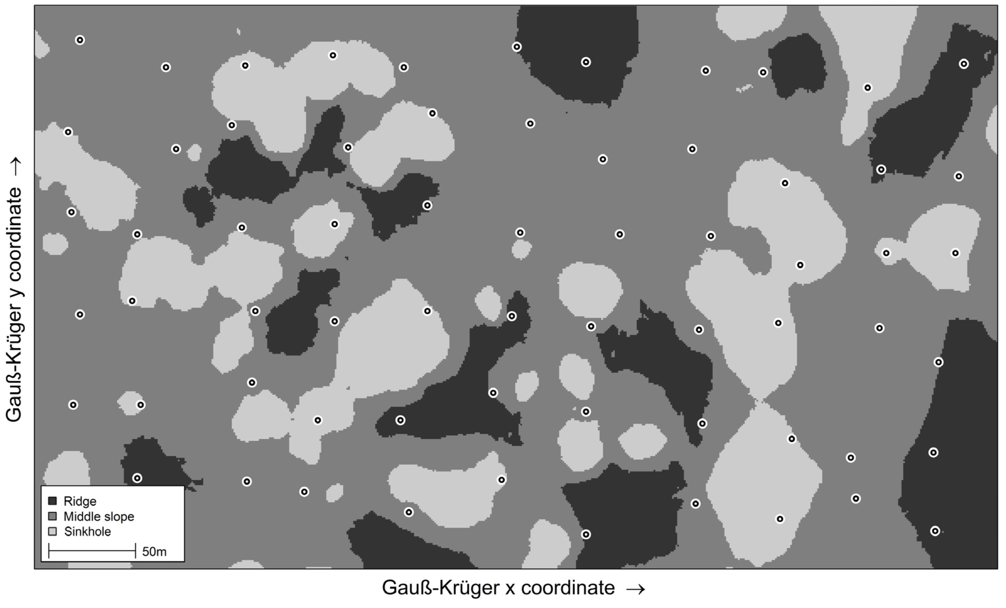
Based on the topographic categories and the differences in the height growth of silver fir trees, we were able to detect terrain-related gradients and landforms within individual tree sites. In a 19.75 ha of the study area, 29 sinkholes and 13 ridges were detected overall using the LiDAR-derived DEM with a cell size of 1 × 1 m (Figure 7).
The middle slopes comprise an area of 12.27 ha (62%), sinkholes have an aggregated area of 4.31 ha (22%), and the aggregated area of ridges is 3.17 ha (16%). The basic morphometric characteristics revealed fine-scale gradients in the study area’s topographic factors, considering that the landform units were delineated within a 50-m-wide elevation zone.
The ridges were detected in landform units with the elevation differences ranging from 3.6 to 14.1 m. Sinkholes smaller than 2000 m2 were delineated as landform units with elevation differences of up to 5 m (12 sinkholes) and up to 10 m (11 sinkholes). In six larger sinkholes with an area of up to 1.10 ha, the maximum sinkhole depth ranged from 11.2 to 21.8 m.
3.3. Differences in the Height Growth and Height Increment of Dominant Silver Fir Trees among Three Landform Categories
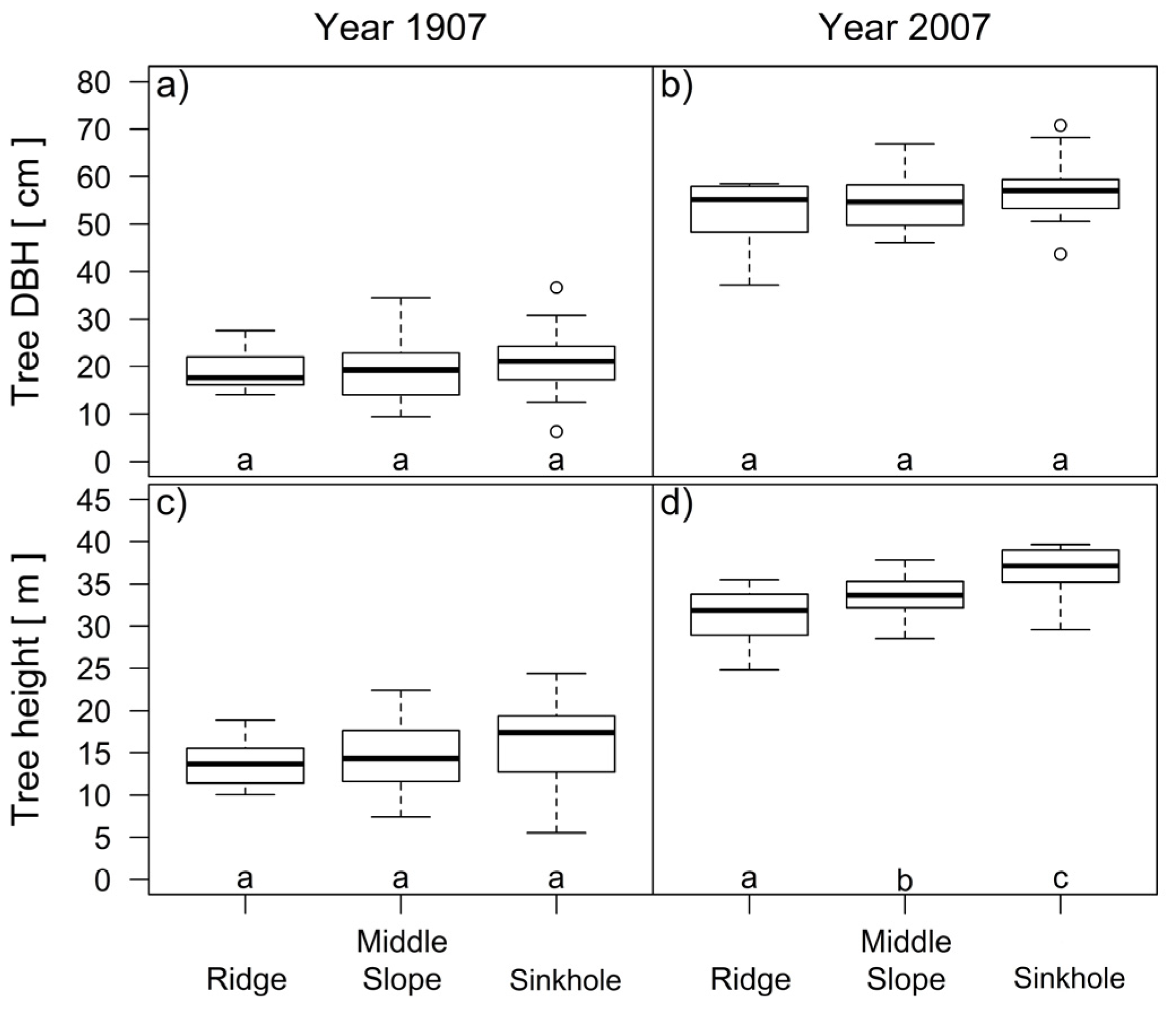
Despite the differences in the height and diameter of the trees, the dendrochronological analysis reveals that there were no significant differences in the ages of the dominant silver fir trees growing on three different landform categories (p = 0.929).
Based on the stem and dendrochronological analysis, we reconstructed the dominant silver fir height growth in the last 100 years. In the period of unsuppressed growth of fir at the beginning of the 20th century, differences in height growth began to increase after the 1950s (Figure 8).
At the beginning of the analyzed period in 1907, the differences in the height and dbh of the trees in the three groups of landform categories were not statistically significant (Figure 9a,c). At the end, in 2007, there were significant differences (p < 0.001) in the tree heights between all three groups of trees (Figure 9d).
The average annual height growth increment between 14 and 24 m of silver fir differs with the landform category (p = 0.008). On average, the silver fir trees in the sinkholes grew 0.28 m/year, the firs on the middle slope grew 0.26 m/year and the firs on the ridges grew 0.21 m/year. The average growth increments of the silver fir trees in the sinkholes and the firs on the middle slope did not significantly differ (p = 0.804), but there were significant differences (p < 0.05) between the trees on the ridges and in sinkholes.
4. Discussion
The results suggest that the topographic factors influencing the height growth of silver fir trees can be detected in mature stands where older firs are responsive to landform and site differences. Using topography modelling, we classified silver fir trees into groups (Figure 5) with statistically significant differences in height growth (Figure 8 and Figure 9).
The spatial model based on topographic factors and differences in the height growth of dominant silver fir trees (Figure 7) is not meant to determine growth indices but, rather, illustrates the significance of spatial variability within forest ecotopes. The differences among the heights of dominant silver fir trees were greater than 2 m, differences used in Middle Europe for the purpose of developing yield tables and escalating the differences between estimated growth indices [54,55].
Understanding this variation in the space and growth of trees (Figure 7) is important to forest management, as differences in height growth might serve as the basis for comparing forest site classes and site conditions within forest communities. Recent studies in forest communities (representing the basic units for the evaluation of site indices) have revealed a great variability in estimations [41,43], highlighting the need for the refinement of forest site classifications in selected forest communities and the fact that these communities are defined by the similarities among them, notwithstanding the gradual variations and differences in site conditions. In addition, the problem of spatial variability was highlighted by Skovsgaard and Vanclay [56] when describing the variability of tree heights and the effects of microsite conditions on the growth of individual trees. The gradient and variation in site conditions, influenced by topography and soil, may dampen or reinforce the natural variability in the size of trees due to genetic variation and silvicultural treatment.
In many forest site classifications, the understory vegetation has been used as an indicator of site productivity. In Central Europe, methods for evaluating the ecological characteristics of phytocenoses or plant communities have been developed to assess environmental factors and their gradients [57,58,59,60]. In forestry, growth types are determined based on vegetation and environmental factors are estimated based on the ecological characteristics of plant species. Consequently, plants are used as indicators of the environmental conditions at individual sites. Bergès et al. [61] have shown that different understory vegetation and floristic indices may be relevant to site index and productivity assessment. In the sessile oak (Quercus petraea) stands of northern France, floristic indices and predictions based on climate, topography and physical and chemical soil characteristics were able to explain the same variations in the site index. In contrast, assessments carried out in the high karst research area have shown that the use of understory vegetation in evaluating the differences in site conditions is ineffective [62]. Within the prevailing forest communities, it was not possible to detect differences in microsites or understory vegetation patterns using phytocenological classifications and the Ellenberg indicator values for vegetation. Thus, the understory vegetation could not be used as a valid indicator of tree growth evaluation on such a small scale. The gradient of the ecological factors of understory vegetation was too small to have an impact on the heterogeneous conditions and differences in the described vegetation units. Similarly, as in other research on the vegetation of karst terrain [63], some of the understory vegetation species of high karst areas [62] are only registered if they are growing either in or on the edge of a sinkhole and were not included in the vegetation inventory elsewhere in the research area. An analysis of ecological factors based on phytoindicator values showed very small differences among the site units in beech forests [64]. The floristic similarity among sample units within sites correlated very well with the differences in the site productivity, whereas less than 10% of the variance in floristic composition was explained by site productivity.
Limited options for plant-based indicators are presented in Figure 8. Steam analyses (Figure 2) indicated that the differences in the height growth of silver fir appeared after the transition of the dominant trees during their later development. According to our assumptions, site differences have a more visible influence on the growth of older trees situated within the three different landform categories (Table 1). The hypothesis that growing conditions for individual trees are influenced by topographic factors was confirmed not only by the trees’ significant height differences but also by the height growth increment of the dominant trees. Equally important is the finding that silver firs within the three groups of topographic factors did not differ in their average age. In addition, the differences in these trees’ growth can be attributed to site differences modified by topographic factors, even though the forest stands are classified as uneven-aged. Steam analyses confirmed the findings of previous studies [37], which presupposed at least a 40-year rejuvenation phase for today’s dominant fir trees. In the Leskova dolina FMU, 1500 stems of fir larger than 25 cm dbh were analyzed in the year 1962 to identify the age and periods of suppressed growth. It was estimated that two thirds of all trees regenerated in the period 1814−1850 [37]. In such stand conditions, it is impossible to assess the growth indices using the principles developed for even-aged stands. Based on the stem and dendrochronological analysis, we can estimate, with 95% confidence limits, that the dominant silver trees in our sample regenerated in the period 1824−1833. After a period of suppressed growth, the height differences between the three groups of dominant trees increased (Figure 8) and at the end of the analysis reached height differences of 3.9 m (Table 1, Figure 6 and Figure 9). These differences are comparable to the results in classical surveys of site indices on karts sites. On five plots of 30 × 30 m, placed on the forest site Omphalodo-Fagetum typicum, the site index values (top height at 100 years, SI100) ranged between 22 and 32, and on the site Omphalodo-Fagetum mercurialetosum SI100 was estimated to be between 24 and 28 [47]. In research of growth and yield characteristics of silver fir in Slovenia, the analysis of site productivity showed that site productivity decreases with altitude and surface stoniness, while it is higher on the concave sites [47]. In our research area, the differences in altitude were within 50 m, but the influence of different landforms on height growth were clearly shown (Figure 8 and Figure 9).
The approach adopted here was similar to that used in the development of individual tree growth models in which the data were gathered from the sampling plots of forest inventories [65] or from experimental observations [40]. In individual tree growth models, forest stands are divided into a mosaic of individual trees, thus achieving a much higher resolution when modelling their interactions in the system [40]. Without historical data on stand dynamics, we were not able to analyze how competition for resources varied with tree development or the differences in the neighboring trees of the selected dominant firs. As shown by Coomes and Allen [66], competition for light has a strong influence on the growth of small trees, whereas competition for nutrients affects trees of all sizes. D’Amato and Puettmann [67] noted that the relationship between relative dominance and the growth of dominant trees likely arises from these trees’ competitive advantage in exploiting available resources.
Modelling topographic factors plays an important role in forest ecotopes, where the differences in gradients of ecological factors can be estimated. However, these differences can often not be determined within an area due to the limited numbers of experimental sampling units included in plant indicator or pedological and chemical studies. Topographic characteristics and soil properties may offer insight into the variation in site productivity, but detailed site mapping is often prohibitively expensive for operational use in forest management [56]. This challenge particularly holds true for ecotopes, in which soil development is likely a consequence of differences in microrelief and the disintegration of limestone parent material [68].
Recent studies have shown that the LiDAR system allows for a synoptic view of landforms and topography, which is not possible with field plots alone [69]. Trevisani [70] presented the potential for exploiting the geomorphological information from high-resolution digital terrain models derived from airborne LiDAR surveys in complex morphology, which raises new prospects for regional analyses in alpine environments. Evaluations of the gradients of ecological factors based on indicator values of understory plants have proven to be insufficiently reliable in high karst areas (Figure 3), whereas for the purposes of estimating the ecological factor gradients within forest ecotopes, the growth differences indicated by topographic factors are reliable.
5. Conclusions
Tree height growth modelling based on LiDAR-derived topographic categories proved to be an effective tool for the detection of differences in forest site conditions. We recommend the presented technique to more reliably draw boundaries between site units, defined as the homogeneous parts of forest sites, and to be used for the purposes of estimating tree growth and site indices. The separation of forest sites is made even more difficult within uneven-aged stands, as the concepts underlying site indices were developed for even-aged and pure forest stands.
In forestry, the methodology based on topographic modelling and differences in tree growth can be used in various site conditions primarily affected by differences in terrain-related gradients and landforms. To demonstrate the application of this methodology, we selected a high karst area, where we expected to find substantial differences within forest ecotopes. The findings should not be generally adopted for similar site conditions; rather, they offer a sound basis for the comparison of site differences and the calibration of models for various tree species by estimating site indices and the gradients of ecological factors in forest ecotopes.
Author Contributions
Conceptualization, Milan Kobal and David Hladnik; methodology, Milan Kobal and David Hladnik; software, Milan Kobal and David Hladnik; validation, Milan Kobal and David Hladnik; formal analysis, Milan Kobal and David Hladnik; investigation, Milan Kobal and David Hladnik; resources, Milan Kobal and David Hladnik; data curation, Milan Kobal and David Hladnik; writing—original draft preparation, Milan Kobal and David Hladnik; writing—review and editing, Milan Kobal and David Hladnik; visualization, Milan Kobal and David Hladnik; supervision, David Hladnik; project administration, Milan Kobal and David Hladnik; funding acquisition, Milan Kobal and David Hladnik. All authors have read and agreed to the published version of the manuscript.
Funding
This research was funded by the Slovenian Research Agency (http://www.arrs.gov.si/sl/, accessed on 10 June 2021), a doctoral study grant from Milan Kobal and by a research Grant from the Man-For C. BD. (LIFE 09 ENV/IT/000078). Lidar data was acquired by the Slovenia Forestry Institute projects. The APC was funded by Pahernik foundation.
Data Availability Statement
The data presented in this study are available on request from the corresponding author.
Conflicts of Interest
The authors declare no conflict of interest.
References
- Naveh, Z.; Lieberman, S. Landscape Ecology; Springer: New York, NY, USA, 1984; 356p. [Google Scholar]
- Zonneveld, I.S. The land unit—A fundamental concept in landscape ecology and its applications. Landsc. Ecol. 1989, 3, 67–86. [Google Scholar] [CrossRef]
- Haber, W. Basic Concepts of Landscape Ecology and Their Application in Land Management. Physiol. Ecol. Jpn. 1990, 27, 131–146. [Google Scholar]
- Forman, R.T.T. Land Mosaics; Cambridge University Press: Cambridge, UK, 1995; 632p. [Google Scholar]
- Skovsgaard, J.P.; Vanclay, J.K. Forest site productivity: A review of the evolution of dendrometric concepts for even-aged stands. Forestry 2008, 81, 13–31. [Google Scholar] [CrossRef] [Green Version]
- Bontemps, J.-D.; Bouriaud, O. Predictive approaches to forest site productivity: Recent trends, challenges and future perspectives. Forestry 2014, 87, 109–128. [Google Scholar] [CrossRef]
- Brandl, S.; Mette, T.; Falk, W.; Vallet, P.; Rötzer, T.; Pretzsch, H. Static site indices from different national forest inventories: Harmonization and prediction from site conditions. Ann. For. Sci. 2018, 75, 56. [Google Scholar] [CrossRef] [Green Version]
- Naveh, Z. Introduction to landscape ecology as a practical transdisciplinary science of landscape study, planning and management. In Atti del XXXI Corso di Cultura in Ecologia; Caattaneo, D., Semenzato, P., Eds.; SEDE: San Vito di Cadore, Italy, 1994; pp. 1–48. [Google Scholar]
- Davis, F.W.; Dozier, J. Information Analysis of a Spatial Database for Ecological Land Classification. Photogramm. Eng. Remote Sens. 1990, 56, 605–613. [Google Scholar]
- Franklin, J.; McCullough, P.; Gray, C. Terrain Variables Used for Predictive Mapping of Vegetation Communities in Southern California. In Terrain Analys: Principles and Applications; Wilson, J.P., Gallant, J.C., Eds.; John Wiley & Sons, Inc.: Hoboken, NJ, USA, 2000; pp. 331–354. [Google Scholar]
- Bastian, O.; Steinhardt, U. Development and Perspectives of Landscape Ecology; Kluwer: Dordrecht, The Netherlands, 2002; 498p. [Google Scholar]
- Rasti, B.; Hong, D.; Hang, R.; Ghamisi, P.; Kang, X.; Chanussot, J.; Benediktsson, J.A. Feature Extraction for Hyperspectral Imagery. The evolution from shallow to deep: Overview and toolbox. IEEE Geosci. Remote Sens. Mag. 2020, 4, 60–88. [Google Scholar] [CrossRef]
- Hong, D.; Yokoya, N.; Chanussot, J.; Zhu, X.X. An Augmented Linear Mixing Model to Address Spectral Variability for Hyperspectral Unmixing. IEEE Trans. Image Process. 2019, 28, 1923–1938. [Google Scholar] [CrossRef] [PubMed] [Green Version]
- Hong, D.; Gao, L.; Yao, J.; Zhang, B.; Plaza, A.; Chanussot, J. Graph Convolutional Networks for Hyperspectral Image Classification. IEEE Trans. Geosci. Remote Sens. 2020, 1–13. [Google Scholar] [CrossRef]
- Muster, S.; Elsenbeer, H.; Conedera, M. Small-scale effects of historical land use and topography on post-cultural tree species composition in an Alpine valley in southern Switzerland. Landsc. Ecol. 2007, 22, 1187–1199. [Google Scholar] [CrossRef]
- Matsuura, T.; Suzuki, W. Analysis of topography and vegetation distribution using a digital elevation model: Case study of a snowy mountain basin in northeastern Japan. Landsc. Ecol. Eng. 2013, 9, 143–155. [Google Scholar] [CrossRef]
- Reger, B.; Härig, T.; Ewald, J. The TRM Model of Potential Natural Vegetation in Mountain Forests. Folia Geobot. 2014, 49, 337–359. [Google Scholar] [CrossRef]
- Pfeffer, K.; Pebesma, E.J.; Burrough, P.A. Mapping alpine vegetation using observations and topographic attributes. Landsc. Ecol. 2003, 18, 759–776. [Google Scholar] [CrossRef]
- Dirnboeck, T.; Dullinger, S.; Gottfried, M.; Ginzler, C.; Grabherr, G. Mapping alpine vegetation based on image analysis, topographic variables and Canonical Correspondence Analysis. Appl. Veg. Sci. 2003, 6, 85–96. [Google Scholar] [CrossRef]
- Mihevc, A. Kras morphology. In Slovene Classical Karst—Kras; Kranjc, A., Ed.; ZRC SAZU: Ljubljana, Slovenia, 1997; pp. 43–49. [Google Scholar]
- Urbančič, M.; Simončič, P.; Prus, T.; Kutnar, L. Atlas Gozdnih Tal Slovenije. Zveza Gozdarskih Društev Slovenije, Gozdarski Vestnik, Silva Slovenica; Gozdarski Inštitut Slovenije: Ljubljana, Slovenia, 2005; 100p. [Google Scholar]
- Kobal, M.; Bertoncelj, I.; Pirotti, F.; Dakskobler, I.; Kutnar, L. Using lidar data to analyse sinkhole characteristics relevant for understory vegetation under forest cover—case study of a high karst area in the Dinaric mountains. PLoS ONE 2015, 10, 3. [Google Scholar] [CrossRef] [Green Version]
- Kutnar, L.; Urbančič, M. Vpliv rastiščnih in sestojnih razmer na pestrost tal in vegetacije v izbranih bukovih in jelovo-bukovih gozdovih na Kočevskem. Zb. Gozdarstva Lesar. 2006, 80, 3–30. [Google Scholar]
- Kobal, M.; Grčman, H.; Zupan, M.; Levanič, T.; Simončič, P.; Kadunc, A.; Hladnik, D. Influence of soil properties on silver fir (Abies alba Mill.) growth in the Dinaric Mountains. For. Ecol. Manag. 2015, 337, 77–87. [Google Scholar] [CrossRef] [Green Version]
- Robič, D.; Acetto, M. Ocena rastiščnih razmer na izbrani lokaciji in ekološke implikacije pri prebiralnem gospodarjenju z gozdovi. Gozdarski Vestn. 2002, 60, 343–351. [Google Scholar]
- Hasenauer, H. Concepts within Tree Growth Modelling. In Sustainable Forest Management—Growth Models for Europe; Hasenauer, H., Ed.; Springer: Berlin/Heidelberg, Germany, 2006; pp. 3–17. [Google Scholar] [CrossRef]
- Van Laar, A.; Akça, A. Forest Mensuration; Springer: Dordrecht, The Netherlands, 2010; 383p. [Google Scholar]
- Sturtevant, B.R.; Seagle, S.W. Comparing estimates of forest site quality in old second-growth oak forests. For. Ecol. Manag. 2004, 191, 311–328. [Google Scholar] [CrossRef]
- Curt, T.; Bouchaud, M.; Agrech, G. Predicting site index of Douglas-fir plantations from ecological variables in the Massif Central area of France. For. Ecol. Manag. 2001, 149, 61–74. [Google Scholar] [CrossRef]
- Aertsen, W.; Kint, V.; Orshoven, J.V.; Muys, B. Evaluation of modelling techniques for forest site productivity prediction in contrasting ecoregions using stochastic multicriteria acceptability analysis (SMAA). Environ. Model. Softw. 2011, 26, 929–937. [Google Scholar] [CrossRef] [Green Version]
- Aertsen, W.; Kint, V.; Muys, B.; Orshoven, J.V. Effects of scale and scaling in predictive modelling of forest site productivity. Environ. Model. Softw. 2012, 31, 19–27. [Google Scholar] [CrossRef] [Green Version]
- Kobler, A.; Pfeifer, N.; Ogrinc, P.; Todorovski, L.; Oštir, K.; Džeroski, S. Repetitive interpolation: A robust algorithm for DTM generation from Aerial Laser Scanner Data in forested terrain. Remote Sens. Environ. 2007, 108, 9–23. [Google Scholar] [CrossRef]
- Weishampel, J.F.; Hightower, J.N.; Chase, A.F.; Chase, D.Z.; Patrick, R.A. Detection and morphologic analysis of potential below-canopy cave openings in the karts landscape around the Maya polity of Caracol ising airborne LiDAR. J. Cave Karst Stud. 2011, 73, 187–196. [Google Scholar] [CrossRef]
- Bončina, A.; Diaci, J.; Cenčič, L. Comparison of the two main types of selection forests in Slovenia: Distribution, site conditions, stand structure, regeneration and management. Forestry 2002, 75, 365–373. [Google Scholar] [CrossRef] [Green Version]
- Copernicus. Copernicus Land Monitoring Service. Reference Data: EU-DEM. 2015. Available online: http://land.copernicus.eu/pan-european/satellite-derived-products/eu-dem (accessed on 11 September 2018).
- Agencija RS Za Okolje. LIDAR. Available online: http://gis.arso.gov.si/evode/profile.aspx?id=atlas_voda_Lidar@Arso&culture=en-US (accessed on 23 June 2019).
- Bončina, A.; Gašperšič, F.; Diaci, J. Long-term changes in tree species composition in the Dinaric mountain forests of Slovenia. For. Chron. 2003, 79, 227–232. [Google Scholar] [CrossRef] [Green Version]
- Braun-Blanquet, J. Pflanzensociologie. Grundzüge der Vegetations Kunde; Springer: Wien, Austria; New York, NY, USA, 1964; 865p. [Google Scholar]
- Kobal, M.; Kastelec, D.; Eler, K. Temporal changes of forest species composition studied by compositional data approach. iForest 2017, 10, 729–738. [Google Scholar] [CrossRef] [Green Version]
- Pretzsch, H. Forest Dynamics, Growth and Yield; Springer: Berlin/Heidelberg, Germany, 2009; 664p. [Google Scholar]
- Kotar, M. Zgradba, Rast in Donos Gozda na Ekoloških in Fizioloških Osnovah; Zveza Gozdarskih Društev Slovenije, Zavod za Gozdove Slovenije: Ljubljana, Slovenia, 2005; 500p. [Google Scholar]
- Kotar, M. Volume and Height Growth of Fully Stocked Mature Beech Stands in Slovenia During the Past Three Decades. In Growth Trends in European Forests; Spiecker, H., Mielikäinen, K., Köhl, M., Skovsgaard, J.P., Eds.; Springer: Berlin/Heidelberg, Germany, 1996; pp. 291–312. [Google Scholar]
- Kadunc, A. Prirastoslovne značinosti jelke (Abies alba Mill.) v Sloveniji. Gozdarski Vestn. 2010, 68, 403–422. [Google Scholar]
- Koivuniemi, J.; Korhonen, K.T. Inventory by Compartments. In Forest Inventory—Methodology and Applications; Kangas, A., Maltamo, M., Eds.; Springer: Dordrecht, The Netherlands, 2009; pp. 271–278. [Google Scholar]
- Levanič, T. A new system for image acquisition in dendrochronology. Tree Ring Res. 2007, 63, 117–122. [Google Scholar] [CrossRef] [Green Version]
- Guay, R.; Gagnon, R.; Morin, H. MacDENDRO, a new automatic and interactive tree ring measurement system based on image processing. In Tree Rings and Environment, Proceedings of the International Dendrochronological Symposium, Ystad, Sweden, 3–9 September 1990; Lundqua Report; Lund University, Department of Quaernary Geology: Lund, Sweden, 1992; pp. 128–129. [Google Scholar]
- Baillie, M.G.L.; Pilcher, J.R. A simple cross-dating programme for tree-ring research. Tree Ring Bull. 1973, 33, 7–14. [Google Scholar]
- R Development Core Team. R: A Language and Environment for Statistical Computing; R Foundation for Statistical Computing: Vienna, Austria, 2019; ISBN 3-900051-07-0. [Google Scholar]
- Carmean, W.H. Site index curves for upland oaks in the central states. For. Sci. 1972, 18, 109–120. [Google Scholar] [CrossRef]
- Sharma, R.P.; Brunner, A.; Eid, T.; Øyen, B.H. Modelling dominant height growth from national forest inventory individual tree data with short time series and large age errors. For. Ecol. Manag. 2011, 262, 2162–2175. [Google Scholar] [CrossRef]
- Cunningham, D.; Grebby, S.; Tansey, K.; Gosar, A.; Kastelic, V. Application of airborne LiDAR to mapping seismogenic faults in forested mountainous terrain, SE Alps, Slovenia. Geophys. Res. Lett. 2006, 33, L20308. [Google Scholar] [CrossRef] [Green Version]
- Weiss, A. Topographic Position and Landforms Analysis. Poster Presentation. In Proceedings of the ESRI User Conference, San Diego, CA, USA, 9–13 July 2001. [Google Scholar]
- Jenness, J. Topographic Position Index (tpi_jen.avx) Extension for ArcView 3.2, v. 1.3a; Jenness Enterprises: Flagstaff, AZ, USA, 2006. [Google Scholar]
- Badoux, E. Ertragstafeln für Fichte, Tanne, Buche und Lärche; Eidgenössische Anstalt für das Forstliche Versuchswesen, (WSL): Zürich, Switzerland, 1969. [Google Scholar]
- Halaj, J.; Grék, J.; Pánek, F.; Petráš, R.; Řehák, J. Rastové Tabuľky Hlavných Drevín ČSSR; Príroda: Bratislava, Slovakia, 1987; 361p. [Google Scholar]
- Skovsgaard, J.P.; Vanclay, J.K. Forest site productivity: A review of spatial and temporal variability in natural site conditions. Forestry 2013, 86, 305–315. [Google Scholar] [CrossRef]
- Landolt, E. Oekologische Zeigerwerte der Schweizer Flora; Veröffentlichungen des Geobotanischen Institutes der ETH, Stiftung Rübel: Zürich, Switzerland, 1977; Volume 46, 208p. [Google Scholar]
- Ellenberg, H.; Weber, E.H.; Düll, R.; Wirth, V.; Werner, W.; Paulissen, D. Zeigerwerte von Pflanzen in Mitteleuropa; Scripta Geobotanika: Göttingen, Germany, 1991; 248p. [Google Scholar]
- Košir, Ž. Vrednotenje Proizvodne Sposobnosti Gozdnih Rastišč in Ekološkega Značaja Fitocenoz; Ministrstvo za Kmetijstvo in Gozdarstvo RS: Ljubljana, Slovenia, 1992; 58p.
- Landolt, E.; Bäumler, B.; Erhardt, A.; Hegg, O.; Klötzli, F.; Lämmler, W.; Nobis, M.; Rudmann-Maurer, K.; Schweingruber, F.; Theurillat, J.-P.; et al. Flora Indicativa. Ökologische Zeigerwerte und Biologische Kennzeichen zur Flora der Schweiz und der Alpen; Editions des Conservatoire et Jardin Botaniques de la Ville de Genève; Haupt-Verlag: Bern, Switzerland; Stuttgart, Germany; Wien, Austria, 2010; 378p. [Google Scholar]
- Bergès, L.; Gégout, J.C.; Franc, A. Can understory vegetation accurately predict site index? A comparative study using floristic and abiotic indices in sessile oak (Quercus petraea Liebl.) stands in northern France. Ann. For. Sci. 2006, 63, 31–42. [Google Scholar] [CrossRef]
- Kobal, M. Vpliv sestojnih, Talnih in Mikrorastiščnih Razmer na Rast in Razvoj Jelke (Abies Alba Mill.) na Visokem Krasu Snežnika. Ph.D. Thesis, Univerza v Ljubljani, BF, Ljubljana, Slovenia, 2011; 148p. [Google Scholar]
- Bátori, Z.; Körmöczi, L.; Erdős, L.; Zalatnai, M.; Csiky, J. Importance of karst sinkholes in preserving relict, mountain, and wetwoodland plant species under sub-Mediterranean climate. A case study from southern Hungary. J. Cave Karst Stud. 2012, 74, 127–134. [Google Scholar] [CrossRef]
- Kotar, M.; Robič, D. Povezanost proizvodne sposobnosti bukovih gozdov v Sloveniji z njihovo floristično sestavo. Gozdarski Vestn. 2001, 59, 227–247. [Google Scholar]
- Monserud, R.A.; Sterba, H. A basal area increment model for individual trees growing in even- and uneven-aged forest stands in Austria. For. Ecol. Manag. 1996, 80, 57–80. [Google Scholar] [CrossRef]
- Coomes, D.A.; Allen, R.B. Effects of size, competition and altitude on tree growth. J. Ecol. 2007, 95, 1084–1097. [Google Scholar] [CrossRef]
- D’Amato, A.W.; Puettmann, K. The relative dominance hypothesis explains interaction dynamics in mixed species Alnus rubra/Pseudotsuga menziesii stands. J. Ecol. 2004, 92, 450–463. [Google Scholar] [CrossRef]
- Furlani, S.; Cucchi, F.; Forti, F.; Rossi, A. Comparison between coastal and inland Karst limestone lowering rates in the northeastern Adriatic Region (Italy and Croatia). Geomorphology 2009, 104, 73–81. [Google Scholar] [CrossRef]
- Zald, H.S.J.; Spies, T.A.; Huso, M.; Gatziolis, D. Climatic, landform, microtopographic, and overstory canopy controls of tree invasion in a subalpine meadow landscape, Oregon Cascades, USA. Landsc. Ecol. 2012, 27, 1197–1212. [Google Scholar] [CrossRef] [Green Version]
- Trevisani, S.; Cavalli, M.; Marchi, L. Surface texture analysis of a high-resolution DTM: Interpreting an alpine basin. Geomorphology 2012, 161–162, 26–39. [Google Scholar] [CrossRef]
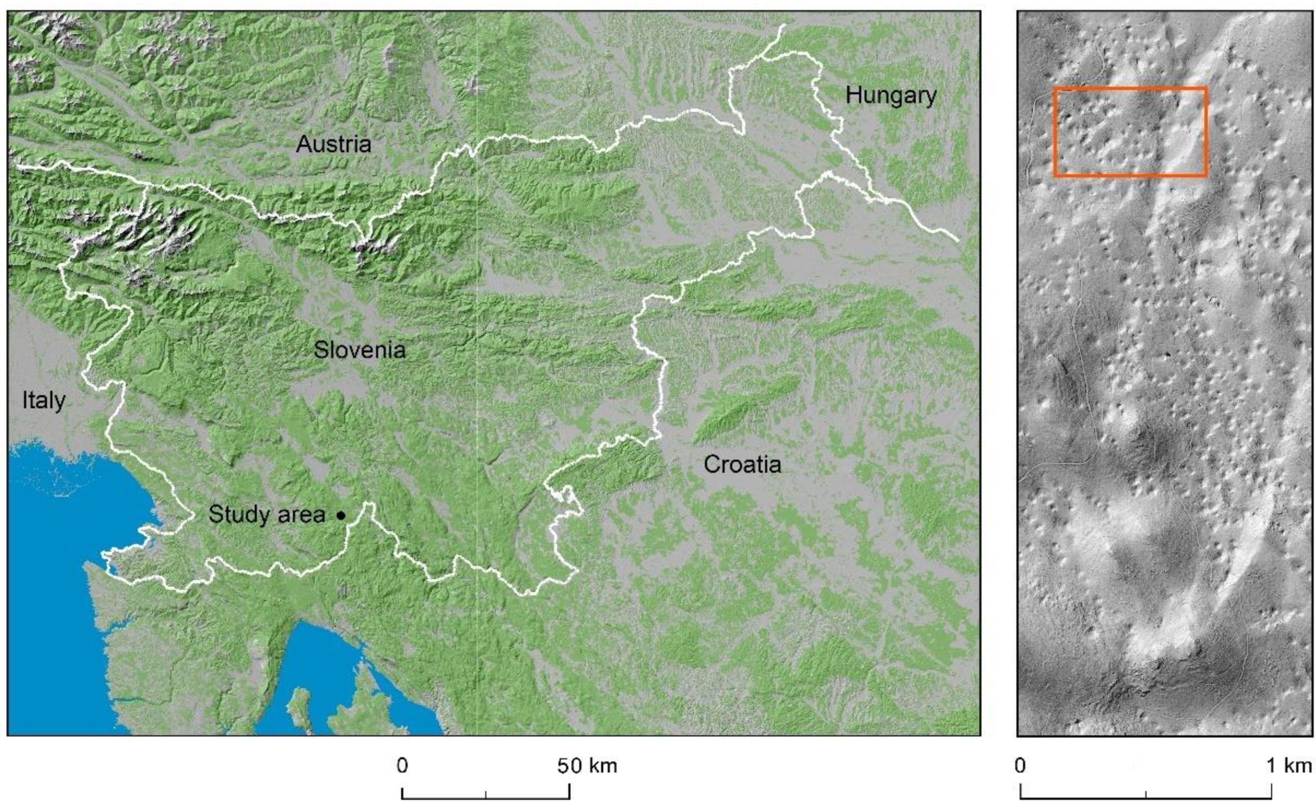
Figure 1.
Location of study area in the Dinaric Mountains presented on a section of the shaded relief of the Digital Elevation Model over Europe [35] and right: the research area as seen from a section of the shaded relief of the Digital Terrain Model (DTM) of Slovenia [36].

Figure 2.
Example of the graphical output from the code for stem analysis, written in the R programing language. Top left: tree ring width series (a); middle left: diameter growth (b); bottom left: height growth increment (c); and right: stem analysis for selected silver fir with marked stem disks and 5-year increments (d).

Figure 3.
A section from LiDAR DEM 1 × 1 m. Gray lines indicate the 50 × 50 m sampling grid, black squares indicate centers of sampling plots from which dominant silver fir trees were selected.
Figure 3.
A section from LiDAR DEM 1 × 1 m. Gray lines indicate the 50 × 50 m sampling grid, black squares indicate centers of sampling plots from which dominant silver fir trees were selected.

Figure 4.
Relief amplitudes (a) and differences between elevations at the base point position of the silver firs and the average elevation differences on their growth sites (b). Note that for different radii, trees are ordered according to amplitudes (a) or differences between the elevation at the base point of silver fir and the average elevation on its growth sites (b).

Figure 5.
Flowchart of the methodology used for delineation of landform categories and modelling dominant silver fir height growth.
Figure 5.
Flowchart of the methodology used for delineation of landform categories and modelling dominant silver fir height growth.
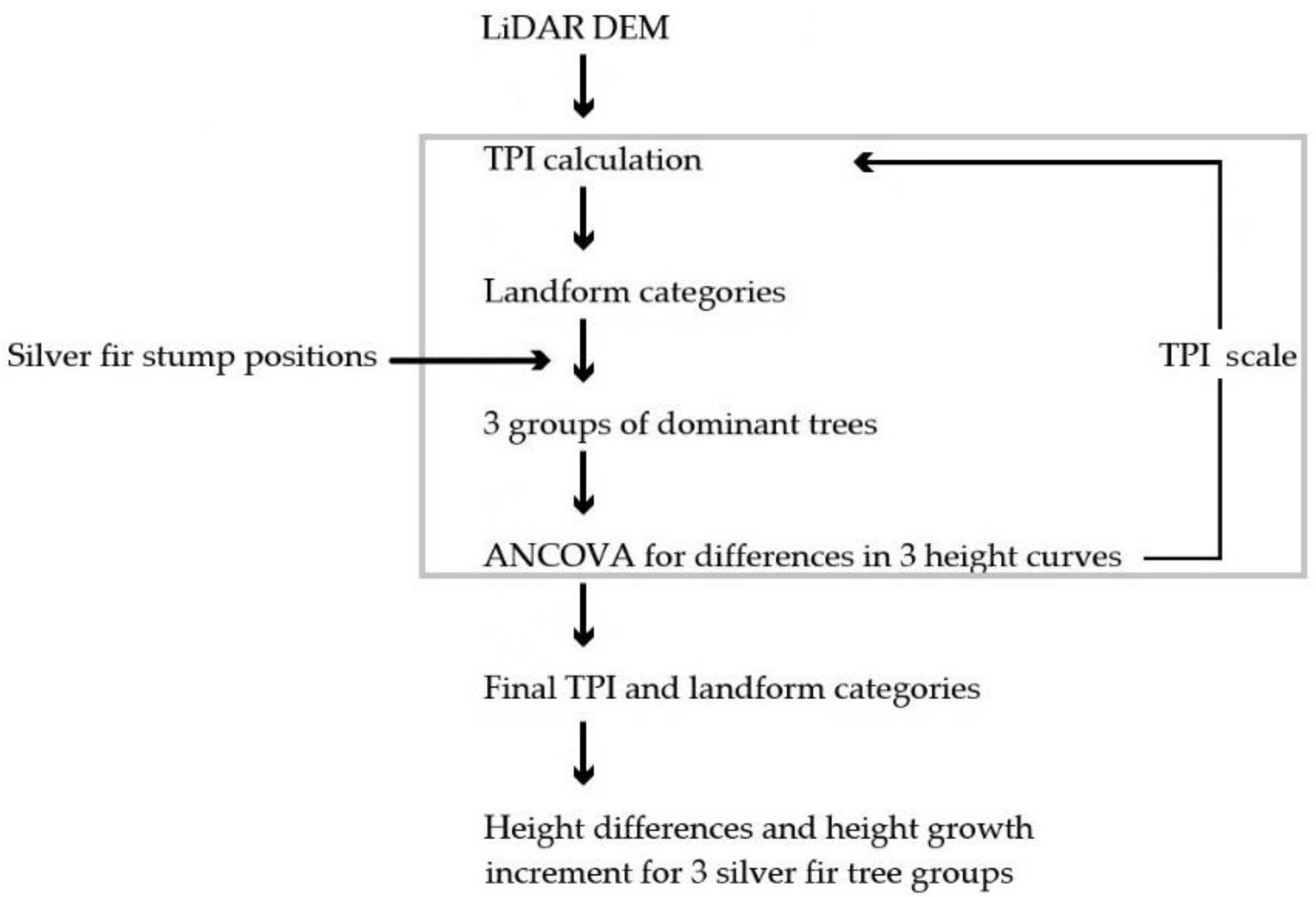
Figure 6.
Changing the adjusted R-Squared in the iterative process of modelling the growth site size according to the height differences of silver fir in the three groups of the landform categories (a). Height curves of the silver fir trees in the three landform categories after the final selection of the scale and delineation of landform categories (b).
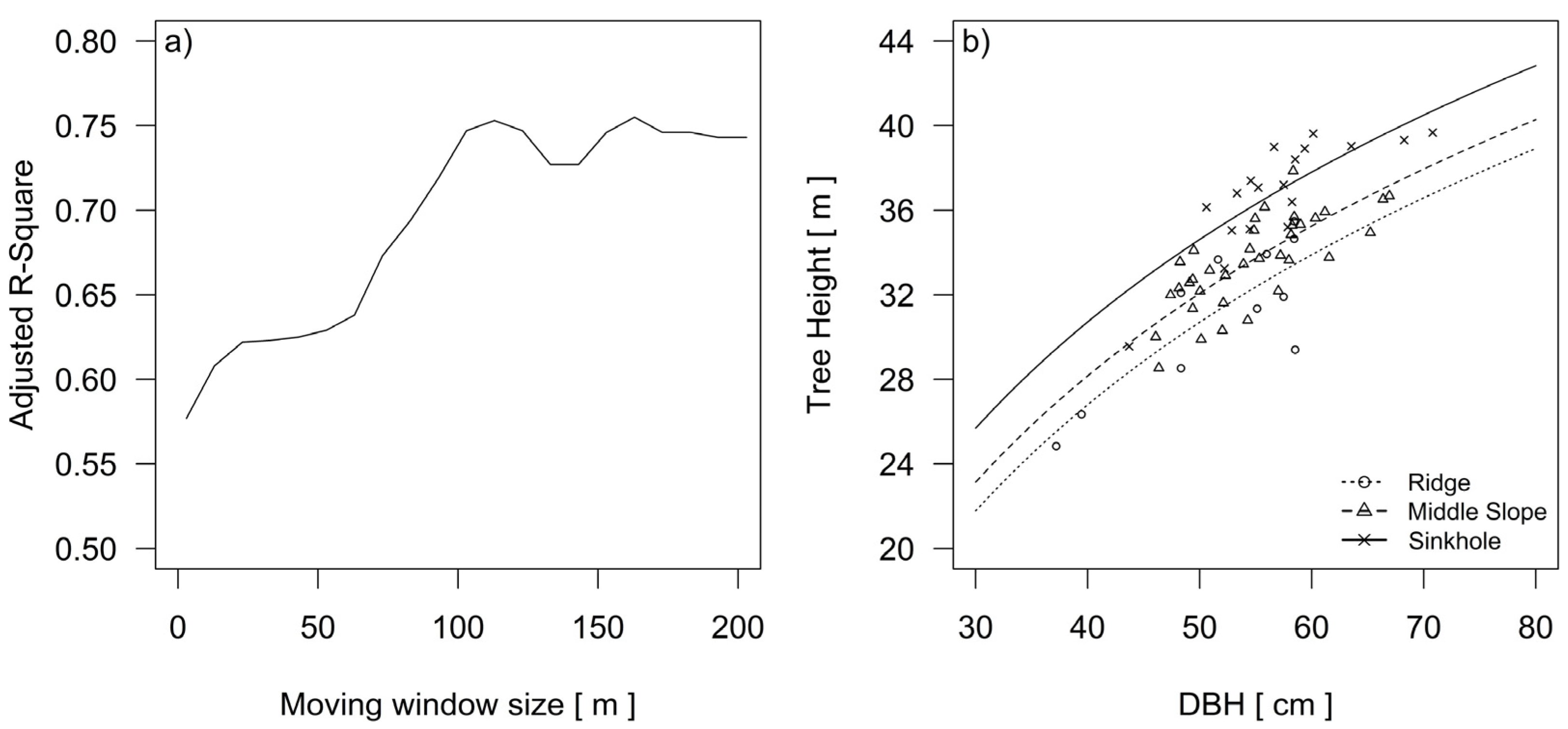
Figure 7.
Spatial model of topographic conditions based on differences in the two models of silver fir tree dominant height and optimal moving window size in the high karst study area. Circles indicate stump positions of the investigated silver fir trees that grew on different landform categories.
Figure 7.
Spatial model of topographic conditions based on differences in the two models of silver fir tree dominant height and optimal moving window size in the high karst study area. Circles indicate stump positions of the investigated silver fir trees that grew on different landform categories.

Figure 8.
The development of height differences for 3 silver fir tree groups after the period of suppressed fir growth. The 95% confidence interval is shown.
Figure 8.
The development of height differences for 3 silver fir tree groups after the period of suppressed fir growth. The 95% confidence interval is shown.

Figure 9.
Comparison of the tree diameters (a,b) and tree heights (c,d) of silver fir trees on different landform categories 100 years ago and at the time of this study. Different letters in figure (d) indicate significant differences (Tukey’s HSD test, p < 0.05) in tree heights between all three groups of trees on ridge, middle slope and sinkhole categories in 2007.

Table 1.
Results of the regressions between silver fir tree height and silver fir dbh without considering landform categories (M1) and considering landform categories (M2).
Table 1.
Results of the regressions between silver fir tree height and silver fir dbh without considering landform categories (M1) and considering landform categories (M2).
| Name | Model | Height Curve | SE | Adjusted R2 | AIC |
|---|---|---|---|---|---|
| M1 | All | H = −48.53 + 20.65 × ln(dbh) | 2.04 | 0.56 | 280.89 |
| Ridge | H = −37.68 + 17.48 × ln(dbh) | ||||
| M2 | Middle slope | H = −36.32 + 17.48 × ln(dbh) | 1.55 | 0.75 | 247.67 |
| Sinkhole | H = −33.76 + 17.48 × ln(dbh) |
Publisher’s Note: MDPI stays neutral with regard to jurisdictional claims in published maps and institutional affiliations. |
© 2021 by the authors. Licensee MDPI, Basel, Switzerland. This article is an open access article distributed under the terms and conditions of the Creative Commons Attribution (CC BY) license (https://creativecommons.org/licenses/by/4.0/).
Share and Cite
MDPI and ACS Style
Kobal, M.; Hladnik, D. Tree Height Growth Modelling Using LiDAR-Derived Topography Information. ISPRS Int. J. Geo-Inf. 2021, 10, 419. https://0-doi-org.brum.beds.ac.uk/10.3390/ijgi10060419
AMA Style
Kobal M, Hladnik D. Tree Height Growth Modelling Using LiDAR-Derived Topography Information. ISPRS International Journal of Geo-Information. 2021; 10(6):419. https://0-doi-org.brum.beds.ac.uk/10.3390/ijgi10060419
Chicago/Turabian StyleKobal, Milan, and David Hladnik. 2021. "Tree Height Growth Modelling Using LiDAR-Derived Topography Information" ISPRS International Journal of Geo-Information 10, no. 6: 419. https://0-doi-org.brum.beds.ac.uk/10.3390/ijgi10060419
Note that from the first issue of 2016, this journal uses article numbers instead of page numbers. See further details here.