Domain Adaptation for Semantic Segmentation of Historical Panchromatic Orthomosaics in Central Africa

Abstract

Multitemporal environmental and urban studies are essential to guide policy making to ultimately improve human wellbeing in the Global South. Land-cover products derived from historical aerial orthomosaics acquired decades ago can provide important evidence to inform long-term studies. To reduce the manual labelling effort by human experts and to scale to large, meaningful regions, we investigate in this study how domain adaptation techniques and deep learning can help to efficiently map land cover in Central Africa. We propose and evaluate a methodology that is based on unsupervised adaptation to reduce the cost of generating reference data for several cities and across different dates. We present the first application of domain adaptation based on fully convolutional networks for semantic segmentation of a dataset of historical panchromatic orthomosaics for land-cover generation for two focus cities Goma-Gisenyi and Bukavu. Our experimental evaluation shows that the domain adaptation methods can reach an overall accuracy between 60% and 70% for different regions. If we add a small amount of labelled data from the target domain, too, further performance gains can be achieved.

1. Introduction

Remote sensing datasets provide the capability to map land-cover which is useful for environmental and urban-related studies [1,2]. A set of remote sensing data collected over a, possibly large, window of time enables to study the historic evolution of the landscape. Thus, multitemporal studies often must make use of both recent imagery and historical datasets. In the mid-20th century, panchromatic aerial photographs were the main source of high spatial resolution imagery [3]. During the colonial era in Africa, the authorities conducted multiple air survey campaigns and generated topographical maps at different scales. The availability and completeness of these datasets has been affected by several factors such as the political course of a country after independence, and the administration of the relevant surveying departments. The availability of archives of historical orthomosaics provides the capability to reconstruct the historical urban developments of these cities. This is a challenging task especially since some of the widely used global datasets only start from the 1970s and have coarse spatial resolutions [4]. With the rapid population growth rates, it is projected that over 22% of the world’s urban population will be residing in Africa by the year 2050, creating implications on infrastructure, demand for housing and environmental degradation [5].

The sustainable development goals (SDGs) are a set of 17 targets that provide a pathway towards a peaceful and prosperous planet by the year 2030 for both the developed and developing countries [6]. Most of the issues it seeks to address exhibit adverse effects that are imbalanced mostly towards countries in the Global South. At the core of the SDGs actions, there lies a great need for adequate data necessary for their monitoring and implementation, among which earth observation is a valuable component [7,8]. In addition to satellite imagery, historical orthomosaics are a pertinent source of spatial data for addressing some of the SDG actions. For instance, SDG 15 is concerned with life on land and addresses issues such as deforestation and land degradation. In this framework, Dewitte et al. [9] explores the benefit of incorporating historical orthomosaics to understand the occurrence and evolution of landslides, and the implied risks on populations. In Depicker et al. [10], the link between deforestation, population dynamics and landslide is analysed for 58 years facilitated by the information from historical orthomosaics. The SDG 11 is concerned with “making cities and human settlements inclusive, safe, resilient and sustainable”. To this end, urban land-cover maps from historical orthomosaics [11] provide the necessary spatial data that aids in understanding the urban growth patterns that can be analysed over a long period, including the different drivers. This kind of information is useful in informing policies regarding the well-being and quality of life of the city resident. From the foregoing, efficient processing algorithms are needed, and are vital for the accurate and timely extraction of land-cover information from historical orthomosaics, that would eventually contribute towards the SDG goals, especially in the Global South.

In the exploitation of historical orthomosaics, some pertinent issues arise. First, historical panchromatic photos have limited spectral information because they have a single channel. This is often a limiting factor when presented with the task of extracting multi-temporal land-cover classes. However, the use of texture features, also referred to as hand-engineered features, can often mitigate against limited spectral information [12]. Secondly, the quality of the images is sensitive to the duration and condition of storage. Furthermore, artefacts can arise during scanning, and intentional or accidental physical marks by the personnel handling the orthomosaics. Different methods have been used to extract land-cover from these images. While photointerpretation is a reliable method for land-cover extraction, it is laborious and non-scalable. On the other hand, a range of machine learning methods reduce the time taken to generate the maps, while increasing efficiency and scalability. Recently, deep learning approaches are being widely applied because they allow for the automatic learning of the feature representations from raw input images as opposed to standard hand-engineering of features [11,13,14,15,16,17,18].

One of the key limitations in remote sensing applications stems from the high budget of preparing reference labelled data. To overcome this issue, several strategies have been explored by the remote sensing community, for example the use of large quantities of freely available but noisy labels from OpenStreetMap [19], collection of labelled data from out-of-date reference maps [20] or applied active learning to gather informative labelled samples from experts [21]. While the above strategies might be appealing, they are not tailored for the analysis of historical images where no reference data, even out-of-date is available and where it is no longer possible to collect field reference data.

For this reason, we explore another well-known strategy used in reducing the amount of training labelled data required: transfer learning. Generally speaking it is a process that utilizes the knowledge learned by solving a task on a source domain to solve another task on a target domain [22,23]. We focus on domain adaptation techniques which are a special case of transfer learning, in the context of classification. In this case a classification model, trained from labelled samples collected in the source domain, is adapted to the target model. It is assumed that a model trained in the source domain would be sub-optimal for classifying the target samples, but still contain useful and discriminative knowledge for the learning task. In remote sensing applications, the shift between the source and target distribution (known as domain shift) might occur due to biased sampling when a region is not representative of a new scene, or due to variations in the acquisition conditions or seasonal changes [21]. Domain adaptation methods aim to reduce these domain shifts caused by spectral, temporal, spatial or radiometric factors. In the domain adaptation framework a set of labelled training data is always available in the source domain; depending on the availability of some labelled data in the target domain, we usually distinguish three scenarios [24]: (1) In an unsupervised domain adaptation scenario, there is only unlabelled data available in the target domain, (2) a semi-supervised domain adaptation scenario assumes that a limited set of labelled samples is available in the target domain, (3) supervised domain adaptation assumes that a substantial set of labelled samples is available in the target domains.

In this work we explore unsupervised domain adaptation using a deep learning-based technique focusing on two methods. Both methods aim at the generation of features that are both invariant and yet discriminative in the source and target domain. The rationale behind the method’s selection is they have the advantage of an easy integration into a deep learning framework, as well as avoiding distortion of data at the raw pixel level space leading to an improved generalisation power at test time [25]. The first approach is the domain adversarial neural network (DANN), which uses an adversarial loss function that aims at predicting domain invariant labels [26] with an example of a binary land-cover application using multi-date and multi-site Landsat satellite imagery [27] and multi-class classification from multispectral and hyperspectral datasets [28]. The second approach is the D-CORAL that reduces the domain shift using the second-order statistics [29] with an example of a different task of object-detection of vehicles from RGB aerial images [30]. Other methods that focus on the alignment of data distribution in the feature space between the source and the target domains but have not been included in this work include the single maximum mean discrepancy (MMD) kernel [31], its multiple variant [32] and optimal transport [33].

Our work is motivated by the need to valorise historical photograph products that are a key component for the understanding of major environmental issues and urban growth studies. We recognise that reduction in the effort of generating reference labels lies at the heart of successfully exploiting historical archives of panchromatic orthomosaics. Therefore, we explore the suitability of unsupervised domain adaptation for semantic segmentation applied to remote sensing images, with a novel use-case on interpretation of historical panchromatic orthomosaics. In addition, we conduct fine-tuning experiments and evaluate the amount of additional reference data needed from the target domain. To the best of our knowledge, it is the first application of domain adaptation that uses a dataset of historical panchromatic orthomosaics. Furthermore, most of the existing works in the remote sensing domain have been conducted using multi-spectral or hyperspectral images, and largely for land-use classification [21,28].

In summary, the objectives of this study are the following: (i) to evaluate and compare two unsupervised domain adaptation methods for the task of land-cover mapping from two historical datasets of panchromatic orthomosaics from the 1940s and 1950s, and (ii) to assess the added benefits of fine-tuning the domain adaptation networks using small amounts of data from the target domain. The rest of the paper is organized as follows: Section 2 provides on overview of the data and the adapted methodology; Section 3 gives the results, and Section 4 the discussion. The conclusion and recommendations are provided in Section 5 followed by an Appendix section (Appendix A).

2. Materials and Methods

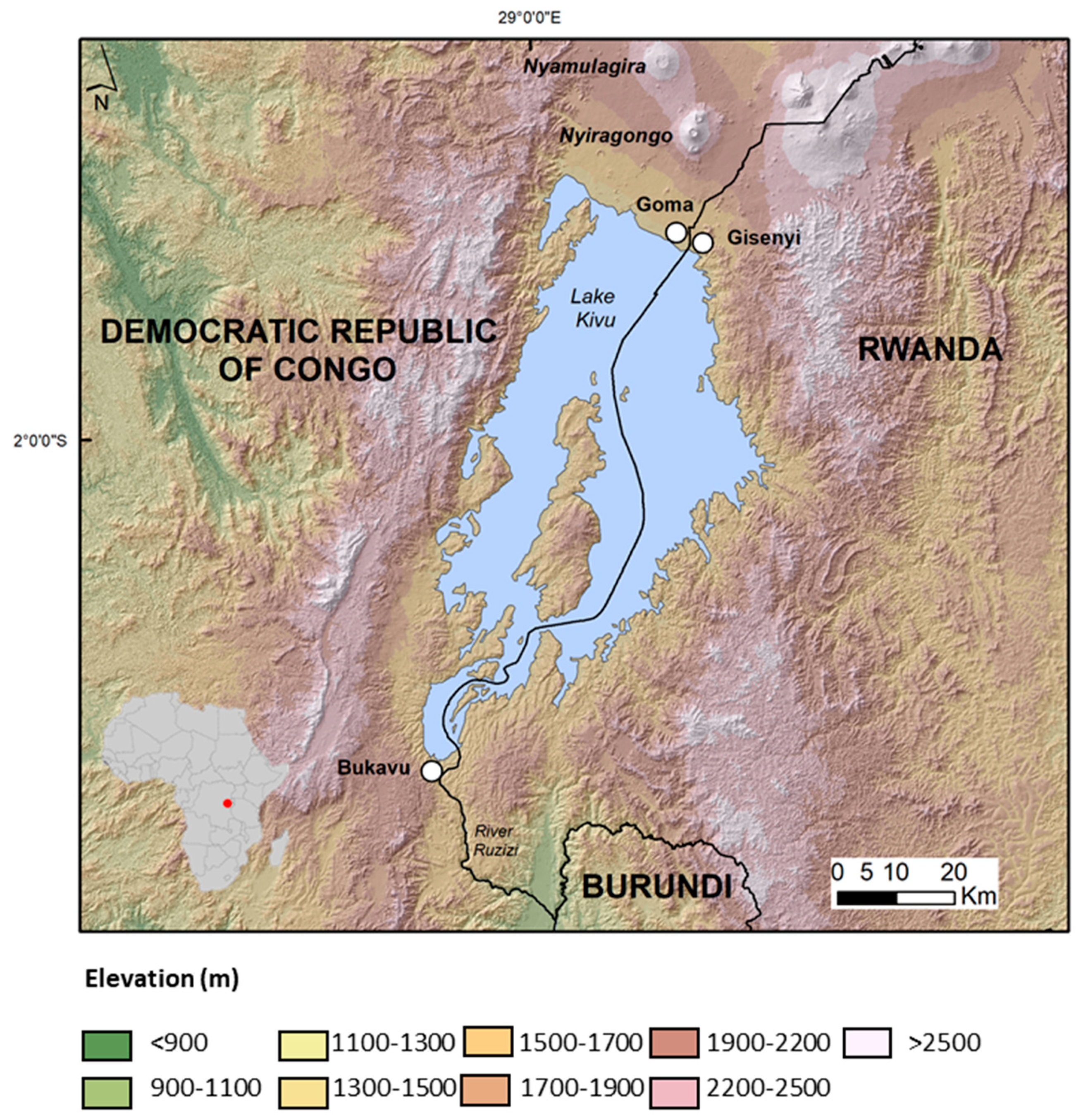
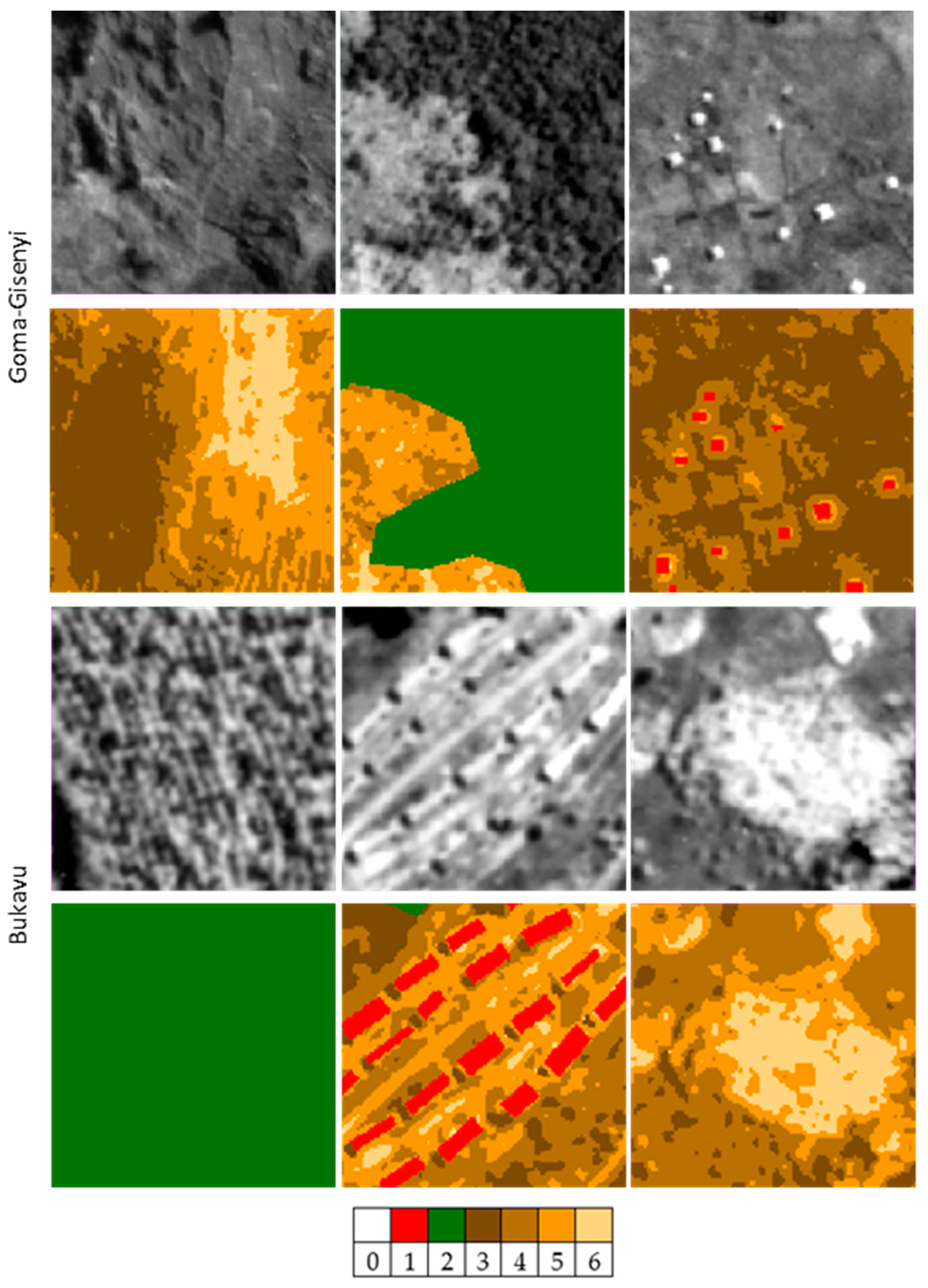
2.1. Data Description

In this work, we use a dataset of historical panchromatic orthomosaics generated from the collections of aerial photographs of the Belgian Royal Museum for Central Africa (see Appendix A). It comprises of images from the city of Goma-Gisenyi (whereby Goma is in the Democratic Republic of Congo and Gisenyi is in Rwanda) captured in 1947, and the city of Bukavu in the Democratic Republic of Congo, captured in 1959 (Figure 1).

These orthomosaics are based on scanned paper reproductions of aerial surveys that were carried out in the 1940s and 1950s in Central Africa. The image pre-processing and photogrammetric processing to obtain the orthomosaics is described in Appendix A. The historical orthomosaics are of limited quality due to several factors. First, camera calibration reports associated with the aerial surveys are missing, which imposes a camera self-calibration of limited quality due to the poor overlapping between the photographs and the limited number of ground control points that can be obtained; the acquisition of accurate and precise ground control points necessary for the camera calibration and the georeferencing of the images is indeed complex, since the landscape nowadays has drastically changed, making difficult the identification of remarkable points visible on both the historical photos and the recent satellite imagery. Hence the final horizontal georeferencing accuracy is of the order of 10.8 to 13.9 m (Appendix A). Secondly, the poor quality of the paper photos makes orthomosaics of limited quality. This is due to low-quality imaging, poor storage conditions, ageing, as well as human-induced damages such as pen marks or scratches. Since the orthomosaics are based on the scanned photos that are already photo-reproductions, blurring, vignetting effects, bad exposure and optical distortions are observed [34]. All these aspects strongly affect the quality of the historical products.

The Goma-Gisenyi orthomosaic has a spatial resolution of 1 m, compared to the 1.1 m resolution of Bukavu. In both cities, the landscape was dominated by high and low vegetation, bare ground and scattered built-up areas. However, Goma-Gisenyi had small-sized buildings as compared to Bukavu. Figure 2 provides sample scenes illustrating examples of panchromatic orthomosaics.

There are several significant sources of domain shift between these two datasets. First, a temporal domain shift exists since the orthomosaics were captured in different years, 1947 and 1959 for Goma-Gisenyi and Bukavu, respectively. A shift in the label/semantic space exists that makes the images structurally different, for instance, the building class appears different between the two images. In addition, the mixed bare ground and low vegetation classes are diverse across both images which can be attributed to differences in lithology of the two cities whereby soils in Goma are black while those in Bukavu are red [35,36]. This combination of several domains shifts makes this task challenging.

The orthomosaics are panchromatic and have a single channel which implies there is limited spectral information for the discrimination of classes. Therefore, any changes to the magnitudes and distribution of the grey values can affect the discrimination ability of the classifier. For example, brightening one image to match its histogram to that of a second image might reduce the size of the shift in the global visual domain but end up distorting the classification accuracy resulting in a particular class being likely mislabelled. These differences present a huge challenge to reducing the domain shift between the historical datasets. For these reasons, including the limited quality of the images, domain adaptation for pixel-wise land-cover classification using this dataset presents a unique situation.

2.2. Domain Adaptation Networks

For semantic segmentation of historical aerial images, we aim to generate domain invariant yet discriminative features at the representation level. Two promising works to build upon for our task of land-cover mapping are the correlation alignment (D-CORAL) domain adaptation network [29] and the domain adversarial neural (DANN) [26]. Both methods can be readily integrated into a deep learning framework, and operate at the feature (representation) level, hence generalisable at the inference stage. Please note that DANN has already been used successfully with remote sensing data (Landsat-8 images [27] and hyperspectral images [28]), and D-CORAL for object-detection from aerial RGB images [30], but neither was used with historical panchromatic orthomosaics.

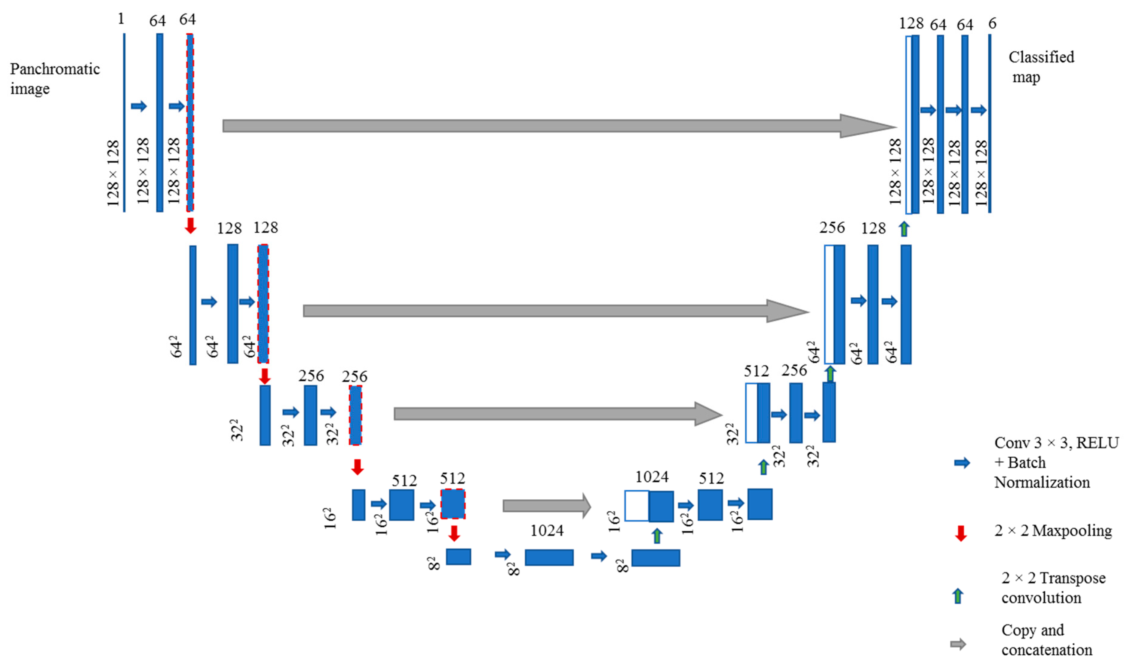
2.2.1. The U-Net Architecture

Similar to Mboga et al. [11] which used a U-Net architecture for supervised land-cover mapping from historical orthomosaics, we use U-Net [37] as the base architecture (Figure 3) in this work. The network has a classical bottleneck architecture consisting of downsampling and upsampling branches with skip connections at each corresponding level. The U-Net has been widely used for remotely sensed imagery [38,39]. Each encoding block is composed of two convolutional layers. Maxpooling layers with a window size of 2 × 2 enable downsampling while transpose convolutions are used for upsampling. Input patches with a dimension of 128 × 128 pixels are fed into the network. The network produces a prediction for each pixel of the input patch. In each of the convolutional layers, rectified linear unit (ReLU) activation functions are used to introduce nonlinearities into the network.

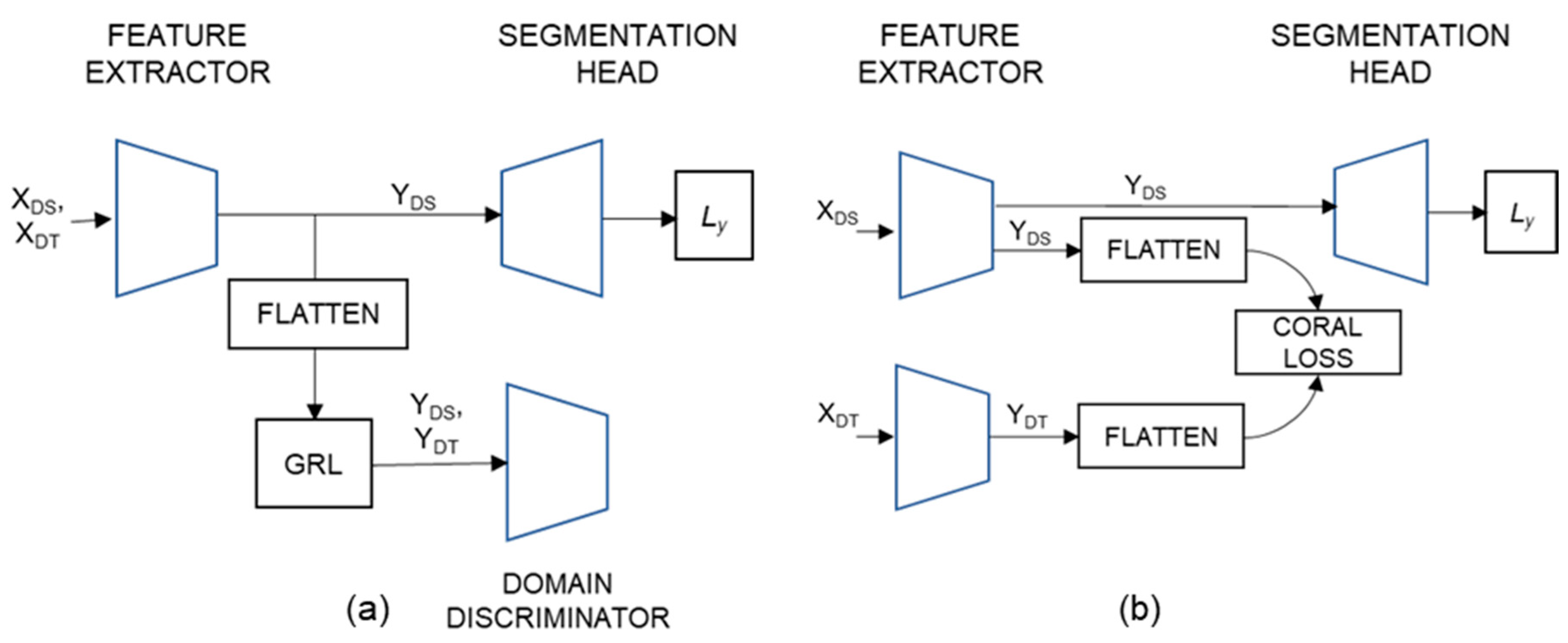
2.2.2. The Domain Adaptation Network

The domain adversarial neural network (DANN) aims to learn class labels that are domain invariant (Figure 4a). It achieves this through the generation of domain invariant and discriminative features [26]. The network contains an encoder (feature extractor), a decoder (segmentation head), and a discriminator. The discriminator determines whether a sample is originating from the source or target domain. DANN utilizes an adversarial loss composed of two main terms: (1) a supervised semantic segmentation loss to be minimized that computes the classical cross-entropy loss on source data, (2) the domain discrimination loss to be maximized, that aims at determining from which domain originates the training data.

The encoder and decoder branches are adapted from the U-Net architecture [37] while the domain discriminator is made of a fully connected network comprising of 100 filters. The training of the network is possible thanks to the gradient reversal layer (GRL), which is added to the network in between the end of the encoder and the start of the discriminator. During the forward pass it acts similar to an identity function (Equation (1)), and does not modify the data, while during the backward-pass it reverses the gradients (it multiplies its input by −1). According to [26], this can be expressed as:

$$Forward pass: R_{\lambda }\left(y\right)=y$$

(1)

$$Backward pass:\frac{d{R}_{\lambda }}{dy}=-\lambda \left(\tau \right)I$$

(2)

where $I$ is an identity matrix multiplied by a weighting factor $\lambda$ to control the influence of the domain discriminator on the learned features. In our experiments we found that setting this value to 1 produced better results as opposed to varying it as described in the original paper [26]. Further, $y$ represents a feature map that is passed through the layer $R_{\lambda }\left(y\right)$ during forward pass. Lastly, $\frac{d{R}_{\lambda }}{dy}$denotes the gradients computed through backpropagation.

The feature extractor branch is derived from the encoding branch of the U-Net architecture. As illustrated in Figure 4a, a gradient reversal layer is used just before the domain classifier responsible for determining whether a sample belong to the source or target domain. Features from the last bottleneck layer of the encoder are flattened before a gradient reversal layer is applied, and the features passed through a domain classifier comprising of fully connected layers of 100 neurons and a binary cross-entropy loss. A segmentation head is made of the decoding branch of a U-Net and allows for the prediction to have similar dimensions to the input image.

The energy function of the domain adaptation is given by:

$$E\left({\theta }_f,{\theta }_y,{\theta }_d\right)=L_y\left({\theta }_f,{\theta }_y\right)-\lambda L_d\left({\theta }_f,{\theta }_d\right)$$

(3)

where $L_y\left({\theta }_f,{\theta }_y\right)$ is the total loss of the class discriminator against the source domain training samples given by the cross-entropy loss, and $L_d\left({\theta }_f,{\theta }_d\right)$ is the total loss for the domain discriminator against both the source and the target training samples. The parameters ${\theta }_f,{\theta }_y,{\theta }_d$, respectively, represents the parameters learned to map the original input into a new latent space, parameters learned to assign the correct class labels to samples from the source domain, and parameters learned to predict the source/domain of the samples.

2.2.3. The D-CORAL Domain Adaptation Network

In this framework, the correlation alignment metric reduces domain discrepancy using the second order statistics (i.e., covariance) between source and target data (Figure 4b). The objective is to ensure that the final deep features are discriminative enough to train a strong classifier and invariant to the shift between the source and target domain.

Let $C_S$ and $C_T$ be the covariance matrices in the source and target domains, respectively. Let us denote by $D_S$ and $D_T$ the $n_S$ source domain samples and the $n_T$ unlabelled target samples. Covariances matrices can be expressed as follows:

$$C_S=\frac{1}{n_S-1}\left(D_S^{⊺} D_S-\frac{1}{n_S}{\left({\mathbf{1}}^{⊺} D_S \right)}^{⊺} \left({\mathbf{1}}^{⊺} D_S\right)\right)$$

(4)

$$C_T=\frac{1}{n_{T-1}}\left(D_T^{⊺} D_T-\frac{1}{n_T}{\left({\mathbf{1}}^{⊺} D_S \right)}^{⊺} \left({\mathbf{1}}^{⊺} D_S\right)\right)$$

(5)

where $\mathbf{1}$ is a column vector with all elements equal to 1. The CORAL loss can be defined as

$$L_{CORAL}=\frac{1}{4d^2}\parallel C_S-C_T{\parallel }_F^2$$

(6)

where $\parallel ·{\parallel }_F^2$ represents the squared matrix Frobenius norm and d is the dimension of the activation features.

During training both the classification loss (cross-entropy loss) and the CORAL loss are minimised using the equation:

$$\mathrm{L}=L_y+{\displaystyle \sum }_{i=1}^t{\alpha }_i{L}_{CORAL}$$

(7)

where $t$ denotes the number of CORAL loss layers in a deep network and $\alpha$ is a weight that trades off adaptation with the classification accuracy on the source domain. The weight of the CORAL loss is set in a way such that at the end of the training, there is an equal contribution between the CORAL loss and the classification loss. An objective that comprises categorical cross entropy loss $L_y$ helps to prevent the likelihood of the network to learn degenerate or useless features as it attempts to reduce the domain shift between the source and target images.

Similar to DANN, the feature extractor is based on the encoding branch of the U-Net architecture. The CORAL loss is computed from the extracted bottleneck features of the source and the target domain just before the start of the decoding branch. Shared parameters are learned by the encoder branch. The segmentation head is comprised of the decoder branch and allows for the propagation of a supervised signal based on images from the source domain. During training, the coefficient of the coral loss is gradually varied from 0 to 1 using a simple scheme $\alpha =\frac{current epoch}{number of epochs}$.

2.3. Experimental Set-Up

The first set of experiments is conducted using standard U-Net without domain adaptation. Training on data from only the source domain provides the lower bound of test accuracy on the target domain (source only). On the other hand, training on images from the target domain provides the upper bound of the test accuracy on the target domain (target only).

In both domain adaptation strategies, data from the source domain includes the raw images and the corresponding labels, while only the raw images are available for the target domain. Figure 5 shows the location of spatially distributed tiles from which training and testing samples were generated for both Goma-Gisenyi and Bukavu. In total, a dataset of 3000 samples of patch size 128 × 128 pixels is obtained from the tiles designated for training and the distribution is shown in Figure 6. During test time, we use an independent test set based on the tiles designated for testing from the target domain to evaluate the classification accuracy and quality of predicted maps.

We further conduct experiments to evaluate the amount of training samples from the target domain needed to fine-tune a domain adaptation network. This is accomplished to assess the added benefit of domain adaptation in reducing amount of reference labels required in a target domain. For this, a domain adaptation network trained using a combination of 150 labelled samples from the source domain and 150 unlabelled samples from the target domain is fine-tuned using samples from the target domain of three sizes namely 150, 300 and 450 selected from the original sample set of 3000 samples, and the accuracy metrics averaged over five runs.

The networks are trained in 50 epochs, using ADAM optimizer [40] with a learning rate of 0.001, and implemented using python 3.7 and PyTorch deep learning framework. The choice of number of epochs, optimizer and learning rate has been identified as optimal after several trial-and-error tests. We use a computer equipped with an NVIDIA GPU GeForce GTX 1080 with 8 GB of RAM.

3. Results

3.1. Unsupervised Domain Adaptation Results

The accuracy assessment is conducted by computing several metrics namely the producer accuracy (PA), the user accuracy (UA), the F1 score and the overall accuracy. An independent test set was used for the calculation of the accuracy metrics. In

Table 1. Overall accuracy metrics on the target and source domains with domain adaptation (DANN, D-CORAL) and without domain adaptation (source only, target only).

METHOD	Source	Goma-Gisenyi	Bukavu
	Target	Bukavu	Goma-Gisenyi
Target only (upper-bound) %	-	91.28	94.50
DANN %	-	61.30	74.78
D-CORAL %	-	62.56	73.00
Source only (lower-bound) %	-	62.04	72.54

, the overall accuracy (OA) tests are presented. Performance of DANN and D-CORAL domain adaptation methods are quite comparable, and the difference in performance is within plus or minus 2%. Both approaches achieve a slightly higher OA compared to the U-Net without domain adaptation (lower bound). In the case of Goma-Gisenyi to Bukavu, there is a difference of + 0.52% in the overall accuracy with and without domain adaptation. An higher OA value is observed when the domain transfer is from Bukavu to Goma-Gisenyi (~72%) as opposed to from Goma-Gisenyi to Bukavu (~62%). The low gain in classification performance can be explained by the fact that there is a remarkable difference in the scene layout of the two cities in terms of the building sizes, vegetation types and high vegetation.

Table 2. The producer accuracy (PA), user accuracy (UA) and F1 score per class for training with and training without domain adaptation. In (a) the city of Bukavu is the target while in (b) the city of Goma-Gisenyi is the target domain. The legend is 1—building (BD), 2—high vegetation (HV), (3–6) mixed bare land and low vegetation (MBLV). 3000 training samples are used.

-	-	-	U-Net (Upper-Bound)			DANN			D-CORAL			U-Net (Lower-Bound)
Goma-Gisenyi ->Bukavu	Bukavu (Target)		PA %	UA %	F1 %	PA %	UA %	F1 %	PA %	UA %	F1 %	PA %	UA %	F1 %
	BD	Class 1	86.1	66.4	75	9.7	56.4	17	7.2	62.9	13	12.7	56.9	21
	HV	Class 2	97.1	94.5	96	61.8	53.7	58	63.0	53.9	58	65.7	53.3	59
	MBLV	Class 3	90.8	95.9	93	55.4	37.8	45	58.7	39.7	47	51.3	39.7	45
		Class 4	90.1	96.7	93	61.9	68.1	65	61.7	70.9	66	62.7	69.9	66
		Class 5	92	88.6	90	74.5	78.1	76	77.2	78.2	78	74.9	75.7	75
		Class 6	80.3	85.0	83	72.8	76.2	74	75.9	76.0	76	71.1	76.9	74
Bukavu->Goma-Gisenyi	Goma (Target)		-	-	-	-	-	-	-	-	-	-	-	-
	BD	Class 1	79.6	59.2	68	19.6	4.8	8	13.5	7.97	10	9.1	2.4	4
	HV	Class 2	96.1	97.4	97	78.9	98.2	88	75.0	98.6	85	74.1	98.5	85
	MBLV	Class 3	90.2	93.9	92	25.1	59.6	35	26.5	57.5	36	27.0	55.5	36
		Class 4	92.3	89.8	91	86.5	44.1	58	87.2	42.1	57	85.5	41.7	56
		Class 5	92.4	88.8	91	88.4	69.8	78	88.7	67.9	77	90.5	68.2	78
		Class 6	98.2	93.2	96	81.8	86	84	82.8	84.4	84	84.1	86.7	85

presents the test class-wise accuracy metrics. High PA, UA and F1 are observed for the U-Net because of the benefit of training using reference data from the target domain, and these provide an upper bound for the classification metrics. The domain adaptation experiments achieve low performance for the building class, the F1 score achieves values in the order of ~0.1–0.2 for both target domains Goma-Gisenyi and Bukavu. For both domain adaptation methods, a high F1 score is observed for the high vegetation (class 2) and the class 5 and 6 of the mixed bare ground and low vegetation class. In addition, very slight differences are observed in the class-wise metrics between the lower-bound U-Net (no transfer) and both domain adaptation methods. As expected, training with labelled target data (upper bound) produces high F1 score and OA compared to the domain adaptation methods and U-Net (lower-bound).

Figure 7 presents sample scenes of classified images. The first column displays the original panchromatic images, the second one the reference data. The third represents the classified map obtained after training on the target image (upper bound). The fourth and the fifth represent the classified maps from domain adaptation models. The last represents the classified map obtained after training on the source image and then making prediction on the target image (lower bound). We observe that both domain adaptation methods classify the mixed bare land and low vegetation well in row (a). The classification of the building class by the domain adaptation methods in Goma-Gisenyi is more challenging as can be observed in row (b), whereas in row (c) the high vegetation class is well captured. In the city of Bukavu, we observe similar good classification performance on the high vegetation class and the mixed bare land and low vegetation classes in row (d) and row (f). While buildings are classified well in row (d), they are not correctly classified in row (e).

3.2. Fine-Tuning Results

While being able to generalize to the target domain without target labels at training time is certainly desirable, when the task is too complex, as in this case, such approach can lead to non-satisfactory performance. However, it is possible to use domain adaptation techniques such that a lower amount of reference labels is needed to obtain a certain classification performance on the target domain. The results of finetuning DANN and D-CORAL using labelled data of different sample sizes from the target domain, namely Bukavu and Goma-Gisenyi, respectively, are shown in

Table 3. Showing overall accuracy (OA) and F1 scores after finetuning model initially trained using 150 samples of the source and target domain using labelled samples from Bukavu. The results are compared to training the U-Net on only target samples and only source samples.

-	Bukavu Target
Number of Samples	300		450		600
-	OA %	F1 %	OA %	F1 %	OA %	F1 %
U-Net (upper bound- only target training)	79.66	74.4	81.40	76.6	82.99	78.2
DANN (150 from source + rest from target)	76.91	73.4	82.19	77.8	83.16	79
D-CORAL (150 from source + rest from target)	78.78	73.8	80.67	76.4	82.27	77.6
U-Net (lower bound—only source)	63.27	58.4	62.81	57.4	62.84	57.4

and

Table 4. Showing overall accuracy (OA) and F1 scores of after finetuning model initially trained using 150 samples of the source and target domain using labelled samples from Goma-Gisenyi. The results are compared to training the U-Net on only target samples and only source samples.

-	Goma-Gisenyi Target
Number of Samples	300		450		600
-	OA %	F1 %	OA %	F1 %	OA %	F1 %
U-Net (upper bound- only target training)	87.49	79.8	89.15	82.4	89.16	83.8
DANN (150 from source + rest from target)	87.78	79.8	88.59	83	89.70	84.4
D-CORAL (150 from source + rest from target)	86.94	80.4	88.94	84	89.17	83.6
U-Net (lower bound—only source)	72.28	55.6	72.76	58	72.21	54

respectively.

The added advantage of using pretrained networks is observed for the three different sample sizes. There is minimal difference in the OA and F1 metrics between upper bound (i.e., with training only from the target domain samples) and when the weights from unsupervised training from each of the domain adaptation models are used as pre-trained weights. The results mean that pretrained weights are used, then fewer samples from the target domain would be required to achieve a similar or slightly better accuracy performance. For example, when Bukavu is the target domain, see Table 3, OA values of 81.40% and 82.19% is obtained, respectively, for U-Net (upper bound training using only data from the target domain) and DANN when 450 samples are used, respectively. In essence, DANN has been finetuned with an amount of labelled data from the target domain that is 150 less than in the U-Net experiment which used exclusively target samples for training (Table 4) where Goma-Gisenyi is the target domain. For instance, training U-Net on 300 labelled target samples gives an OA of 87.49% while fine-tuning a DANN model with only 150 labelled target samples gives an OA of 87.78%. The results imply that it is plausible to take advantage of pre-trained weights generated through unsupervised domain adaptation to reduce the amount of required labelled data from the target domain

4. Discussion

In this paper, two real-world image datasets from two different cities of Goma-Gisenyi and Bukavu, acquired in 1947 and 1959, respectively, have been utilized. From the experiments, by looking at both the numerical and qualitative results, it is evident that relying exclusively on unsupervised domain adaptation might not always be sufficient to guarantee a certain level of performance in classification accuracy. In Bejiga et al. [27], by using a multi-date, multi-site and multi-spectral dataset, it is observed that the use of domain adaptation for a problem with more than one source of domain shift (i.e., images of different spatial locations and acquired at different time periods) increases the level of challenge in unsupervised domain adaptation approaches, affecting their performance. For remote sensing applications, this implies that there is a need to use domain-specific knowledge [41] that would help to reduce some degree of domain shift, hence augmenting the unsupervised domain adaptation approaches. Most applications in computer vision assume the scene layout between images is comparable with the differences stemming from the spectral characteristics, for example, an image of the street taken in the morning and in the afternoon. A leading assumption in a majority of the domain adaptation experiments is that the differences between the domains are “mainly low-level, that is, differences due to noise, resolution, illumination, colour rather than high-level such as in the types of objects, geometric variations etc.” [42]. On the contrary, a scene in a remote sensing image exhibits a variation in the spatial and structural patterns that increase the level of challenge in the performance of domain adaptation methods. Semantic segmentation of multiple land-cover classes from remote sensing imagery is more challenging than a scene classification because of the variety of categories within a scene. Furthermore, the use of historical panchromatic orthomosaics, evident in this work, complicates the discrimination of classes because of the limited spectral information available. Lastly, due to the quality of the historical orthomosaics used in this work, another possible research direction would to be to investigate effectiveness of the methods on a dataset of higher quality.

5. Conclusions

The reduction in the budget of generating reference labels is essential in remote sensing applications, which are also important to monitoring and implementing SDGs goals. It increases the efficiency of generating land-cover and land-use maps from datasets spanning large geographical extents. To this end, two unsupervised domain adaptation methods, namely, DANN and D-CORAL, are evaluated on a case study focusing on historical panchromatic orthomosaics. According to the conducted experiments we can conclude that unsupervised domain adaptation is not sufficient to generate accurate land-cover maps, however, when combined with a limited amount of reference data it can greatly reduce the labelling effort when compared to a standard supervised learning approach. While long-term baseline studies can benefit from exploiting available archives of historical panchromatic orthomosaics, the challenge of creating adequate reference data for each of the dates remains. This study implies that the use of real-world datasets beyond standard benchmarks highlights a limitation of the state-of-the-art approaches. In addition, the availability and use of multiple, high quality, real-world datasets would serve to test the effectiveness of the proposed approaches. In summary, future works will focus on exploiting a highly specific domain knowledge to address the shift between source and target domains.

References

1. Grippa, T.; Lennert, M.; Beaumont, B.; Vanhuysse, S.; Stephenne, N. An Open-Source Semi-Automated Processing Chain for Urban Object-Based Classification. Remote Sens. 2017, 9, 358. [Google Scholar] [CrossRef] [Green Version]
2. Georganos, S.; Brousse, O.; Dujardin, S.; Linard, C.; Casey, D.; Milliones, M.; Parmentier, B.; van Lipzig, N.P.M.; Demuzere, M.; Grippa, T.; et al. Modelling and mapping the intra-urban spatial distribution of Plasmodium falciparum parasite rate using very-high-resolution satellite derived indicators. Int. J. Health Geogr. 2020, 19, 38. [Google Scholar] [CrossRef]
3. Luman, D.E.; Stohr, C.; Hunt, L. Digital Reproduction of Historical Aerial Photographic Prints for Preserving a Deteriorating Archive. Am. Soc. Photogramm. Remote Sens. 1997, 63, 1171–1179. [Google Scholar]
4. Corbane, C.; Florczyk, A.; Pesaresi, M.; Politis, P.; Syrris, V. GHS-BUILT R2018A—GHS built-up grid, derived from Landsat, multitemporal (1975-1990-2000-2014). Eur. Comm. Jt. Res. Cent. JRC. [Dataset] 2018. [Google Scholar] [CrossRef]
5. United Nations, Department of Economic and Social Affairs, Population Division. World Urbanization Prospects: The 2018 Revision (ST/ESA/SER.A/420). United Nations: New York, NY, USA, 2019. [Google Scholar]
6. UNSTATS Overview—SDG Indicators. Available online: https://unstats.un.org/sdgs/report/2018/overview/ (accessed on 20 May 2021).
7. European Space Agency (ESA). EARTH OBSERVATION FOR SDG Compendium of Earth Observation Contributions to the SDG Targets and Indicators; European Space Agency (ESA): Paris, France, 2020. [Google Scholar]
8. European Space Agency (ESA). Satellite Earth Observations in Support of the Sustainable Development Goals. 2018. Available online: https://data.jrc.ec.europa.eu/dataset/jrc-ghsl-10007 (accessed on 30 May 2021).
9. Dewitte, O.; Dille, A.; Depicker, A.; Kubwimana, D.; Maki Mateso, J.C.; Mugaruka Bibentyo, T.; Uwihirwe, J.; Monsieurs, E. Constraining landslide timing in a data-scarce context: From recent to very old processes in the tropical environment of the North Tanganyika-Kivu Rift region. Landslides 2021, 18, 161–177. [Google Scholar] [CrossRef]
10. Depicker, A.; Jacobs, L.; Mboga, N.; Smets, B.; Van Rompaey, A.; Lennert, M.; Wolff, E.; Kervyn, F.; Michellier, C.; Dewitte, O.; et al. Historical dynamics of landslide risk from population and forest cover changes in the Kivu Rift. Nat. Sustain. 2021, in press. [Google Scholar]
11. Mboga, N.; Grippa, T.; Georganos, S.; Vanhuysse, S.; Smets, B.; Dewitte, O.; Wolff, E.; Lennert, M. Fully convolutional networks for land cover classification from historical panchromatic aerial photographs. ISPRS J. Photogramm. Remote Sens. 2020, 167, 385–395. [Google Scholar] [CrossRef]
12. Caridade, C.M.R.; Marc, A.R.S.; Mendonc, T. The use of texture for image classification of black & white air-photographs. Int. J. Remote Sens. 2008, 29, 593–607. [Google Scholar]
13. Ma, L.; Liu, Y.; Zhang, X.; Ye, Y.; Yin, G.; Johnson, B.A. Deep learning in remote sensing applications: A meta-analysis and review. ISPRS J. Photogramm. Remote Sens. 2019, 152, 166–177. [Google Scholar] [CrossRef]
14. Ball, J.E.; Anderson, D.T.; Chan, C.S. Comprehensive survey of deep learning in remote sensing: Theories, tools, and challenges for the community. J. Appl. Remote Sens. 2017, 11, 42609. [Google Scholar] [CrossRef] [Green Version]
15. Zhu, X.X.; Tuia, D.; Mou, L.; Xia, G.-S.; Zhang, L.; Xu, F.; Fraundorfer, F. Deep Learning in Remote Sensing: A comprehensive review and list of resources. IEEE Geosci. Remote Sens. Mag. 2017, 5, 8–36. [Google Scholar] [CrossRef] [Green Version]
16. Marmanis, D.; Wegner, J.D.; Galliani, S.; Schindler, K.; Datcu, M.; Stilla, U. Semantic Segmentation of Aerial Images with an Ensemble of CNSS. ISPRS Ann. Photogramm. Remote Sens. Spat. Inf. Sci. 2016, 3, 473–480. [Google Scholar] [CrossRef] [Green Version]
17. Li, Z.; Wegner, J.D.; Lucchi, A. Topological map extraction from overhead images. In Proceedings of the IEEE/CVF International Conference on Computer Vision, Seoul, Korea, 27 October–2 November 2019; pp. 1715–1724. [Google Scholar]
18. Bergado, J.R.; Persello, C.; Stein, A. Recurrent Multiresolution Convolutional Networks for VHR Image Classification. IEEE Trans. Geosci. Remote Sens. 2018, 56, 1–14. [Google Scholar] [CrossRef] [Green Version]
19. Kaiser, P.; Wegner, J.D.; Lucchi, A.; Jaggi, M.; Hofmann, T.; Schindler, K. Learning Aerial Image Segmentation from Online Maps. IEEE Trans. Geosci. Remote Sens. 2017, 55, 6054–6068. [Google Scholar] [CrossRef]
20. Tardy, B.; Inglada, J.; Michel, J. Assessment of optimal transport for operational land-cover mapping using high-resolution satellite images time series without reference data of the mapping period. Remote Sens. 2019, 11, 1047. [Google Scholar] [CrossRef] [Green Version]
21. Tuia, D.; Persello, C.; Bruzzone, L. Domain adaptation for the classification of remote sensing data: An overview of recent advances. IEEE Geosci. Remote Sens. Mag. 2016, 4, 41–57. [Google Scholar] [CrossRef]
22. Pan, S.J.; Yang, Q. A Survey on Transfer Learning. IEEE Trans. Knowl. Data Eng. 2010, 22, 1345–1359. [Google Scholar] [CrossRef]
23. Weiss, K.; Khoshgoftaar, T.M.; Wang, D.D. A Survey of Transfer Learning. J. Big Data 2016, 3, 9. [Google Scholar] [CrossRef] [Green Version]
24. Csurka, G. A comprehensive survey on domain adaptation for visual applications. In Domain Adaptation in Computer Vision Applications; Csurka, G., Ed.; Springer International Publishing: Cham, Switzerland, 2017; pp. 1–35. [Google Scholar]
25. Bolte, J.A.; Kamp, M.; Breuer, A.; Homoceanu, S.; Schlicht, P.; Huger, F.; Lipinski, D.; Fingscheidt, T. Unsupervised domain adaptation to improve image segmentation quality both in the source and target domain. In Proceedings of the IEEE/CVF Conference on Computer Vision and Pattern Recognition Workshops, Long Beach, CA, USA, 16–17 June 2019; pp. 1404–1413. [Google Scholar]
26. Ganin, Y.; Ustinova, E.; Ajakan, H.; Germain, P.; Larochelle, H.; Laviolette, F.; Marchand, M.; Lempitsky, V. Domain-Adversarial Training of Neural Networks. J. Mach. Learn. Res. 2016, 17, 1–35. [Google Scholar]
27. Bejiga, M.B.; Melgani, F.; Beraldini, P. Domain adversarial neural networks for large-scale land cover classification. Remote Sens. 2019, 11, 1153. [Google Scholar] [CrossRef] [Green Version]
28. Elshamli, A.; Taylor, G.W.; Areibi, S.; Member, S. Multisource Domain Adaptation for Remote Sensing Using Deep Neural Networks. IEEE Trans. Geosci. Remote Sens. 2019, 58, 3328–3340. [Google Scholar] [CrossRef]
29. Sun, B.; Saenko, K. Deep CORAL: Correlation Alignment for Deep Domain Adaptation. In European Conference on Computer Vision; Springer: Berlin/Heidelberg, Germany, 2016; pp. 443–450. [Google Scholar]
30. Koga, Y.; Miyazaki, H.; Shibasaki, R. A Method for Vehicle Detection in High-Resolution Satellite Images That Uses a Region-Based Object Detector and Unsupervised Domain Adaptation. Remote Sens. 2020, 12, 575. [Google Scholar] [CrossRef] [Green Version]
31. Tzeng, E.; Hoffman, J.; Zhang, N.; Saenko, K.; Darrell, T. Deep Domain Confusion: Maximizing for Domain Invariance. arXiv 2014, arXiv:1412.3474. [Google Scholar]
32. Jordan, M.I.; Edu, J.B. Learning Transferable Features with Deep Adaptation Networks. arXiv 2015, arXiv:1502.02791v2. [Google Scholar]
33. Courty, N.; Flamary, R.; Habrard, A.; Rakotomamonjy, A. Joint distribution optimal transport for domain adaptation. In Proceedings of the European Conference on Computer Vision, Munich, Germany, 8–14 September 2018; pp. 447–463. [Google Scholar]
34. Smets, B.; Dewitte, O.; Michellier, C.; Munganga, G.; Dille, A.; Kervyn, F. Insights into the SfM photogrammetric processing of historical panchromatic aerial photographs without camera calibration information. ISPRS Int. J. Geo-Inform. 2020, in press. [Google Scholar]
35. Dille, A.; Kervyn, F.; Bibentyo, T.M.; Delvaux, D.; Ganza, G.B.; Mawe, G.I.; Buzera, C.K.; Nakito, E.S.; Moeyersons, J.; Monsieurs, E.; et al. Causes and triggers of deep-seated hillslope instability in the tropics—Insights from a 60-year record of Ikoma landslide (DR Congo). Geomorphology 2019, 345, 106835. [Google Scholar] [CrossRef]
36. Michellier, C.; Pigeon, P.; Paillet, A.; Trefon, T.; Dewitte, O.; Kervyn, F. The Challenging Place of Natural Hazards in Disaster Risk Reduction Conceptual Models: Insights from Central Africa and the European Alps. Int. J. Disaster Risk Sci. 2020, 11, 316–332. [Google Scholar] [CrossRef]
37. Ronneberger, O.; Fischer, P.; Brox, T. U-Net: Convolutional Networks for Biomedical Image Segmentation. In International Conference on Medical Image Computing and Computer-Assisted Intervention; Springer: Cham, Switzerland, 2015; pp. 234–241. [Google Scholar]
38. Cao, K.; Zhang, X. An improved Res-UNet model for tree species classification using airborne high-resolution images. Remote Sens. 2020, 12, 1128. [Google Scholar] [CrossRef] [Green Version]
39. Peng, D.; Zhang, Y.; Guan, H. End-to-End Change Detection for High Resolution Satellite Images Using Improved UNet ++. Remote Sens. 2019, 11, 1382. [Google Scholar] [CrossRef] [Green Version]
40. Kingma, D.P.; Ba, J. Adam: A Method for Stochastic Optimization. arXiv 2014, arXiv:1412.6980. [Google Scholar]
41. Tuia, D.; Roscher, R.; Wegner, J.D.; Jacobs, N.; Zhu, X.; Camps-Valls, G. Toward a Collective Agenda on AI for Earth Science Data Analysis. IEEE Geosci. Remote Sens. Mag. 2021, 9, 88–104. [Google Scholar] [CrossRef]
42. Bousmalis, K.; Silberman, N.; Dohan, D.; Erhan, D.; Krishnan, D. Unsupervised pixel-level domain adaptation with generative adversarial networks. In Proceedings of the IEEE Conference on Computer Vision and Pattern Recognition, CVPR, Honolulu, HI, USA, 21–26 July 2017; pp. 95–104. [Google Scholar]
Figure 1. Map of the study area showing the border cities of Goma-Gisenyi at the border of the Democratic Republic of Congo and Rwanda and Bukavu in the Democratic Republic of Congo.
Ijgi 10 00523 g001
Figure 2. Sample training images from Goma-Gisenyi (first two rows) and Bukavu (last two rows) illustrating examples of panchromatic images, and the diversity in the layout and appearance of classes. The legend is 1—building, 2—high vegetation, (3–6) mixed bare land and low vegetation. 0 represents the unclassified pixels.
Ijgi 10 00523 g002
Figure 3. Diagram of U-Net adapted from Mboga et al. [11].
Ijgi 10 00523 g003
Figure 4. Diagrams of the (a) DANN and (b) D-CORAL frameworks.
Ijgi 10 00523 g004
Figure 5. Locations of the training and testing tiles in the images of (a) Bukavu (b) Goma-Gisenyi used in the experiments covering a geographical area of 258 km2 and 80 km2. Adapted from Mboga et al. [11].
Ijgi 10 00523 g005
Figure 6. Distribution of training samples for Goma-Gisenyi and Bukavu. In the legend, 1—building, 2—high vegetation, 3–6 (mixed bare land and low vegetation).
Ijgi 10 00523 g006
Figure 7. Sample classified scenes in Bukavu and Goma-Gisenyi. The legend is 1—building, 2—high vegetation, (3–6) Mixed bare land and low vegetation. 0 represents the unclassified pixels.
Ijgi 10 00523 g007