
Road Network Generalization Method Constrained by Residential Areas


1
Institute of Geospatial Information, Information Engineering University, Zhengzhou 450000, China
2
Collaborative Innovation Center of Geo-Information Technology for Smart Central Plains, Zhengzhou 450000, China
3
Key Laboratory of Spatiotemporal Perception and Intelligent Processing, Ministry of Natural Resources, Zhengzhou 450000, China
*
Author to whom correspondence should be addressed.
ISPRS Int. J. Geo-Inf. 2022, 11(3), 159; https://0-doi-org.brum.beds.ac.uk/10.3390/ijgi11030159
Submission received: 29 December 2021
/
Revised: 17 February 2022
/
Accepted: 18 February 2022
/
Published: 22 February 2022
(This article belongs to the Special Issue Cartography and Geomedia)
Abstract
:Residential areas and road networks have a strong geographical correlation. The development of a single geographical feature could destroy the geographical correlation. It is necessary to establish collaborative generalization models suitable for multiple features. However, existing road network generalization methods for mapping purposes do not fully consider residential areas. Compared with road networks, residential areas have a higher priority in cartographic generalization. In this regard, this study proposes a road network generalization method constrained by residential areas. First, the roads and settlements obtained from clustering residential areas were classified. Next, the importance of the settlements was evaluated and certain settlements were selected as the control features. Subsequently, a geographical network with the settlements as the nodes was built, and the traffic paths between adjacent settlements were searched. Finally, redundant paths between the settlements were simplified, and the visual continuity and topological connectivity were checked. The data of a 1:50,000 road network and residential areas were used as the experimental data. The experimental results demonstrated that the proposed method preserves the overall structure and relative density characteristics of the road network, as well as the geographical correlation between the road network and residential areas.
1. Introduction
Cartographic generalization is a technology and science that produces abstract and generalized spatial data when transferring large-scale map information to small-scale maps [1]. The concept of cartographic generalization was first proposed by Eckert in 1921. After years of development, it has experienced a transformation from “geometric perspective → computational perspective → functional perspective”, and knowledge and semantic information have attracted increasing attention [2]. The map is a complex system formed by a variety of interactive geographical features. The spatial distribution characteristics of different geographical features, as well as the geographical correlation between features, need to be preserved in cartographic generalization. This is because the generalization of a single geographical feature is likely to destroy the geographical correlation between geographical features, resulting in spatial and semantic conflicts between the results [3]. Long experience has proven that the generalization method for a single type of geographical feature cannot adapt to the development of the scientific paradigm of cartographic generalization, so it is necessary to establish a collaborative generalization model directly facing multiple features.
Roads and residential areas are important socioeconomic features on maps. Residential areas are centers of human activity, and accordingly, the material and personnel between residential areas mainly flow through roads. Residential areas and the road network together constitute the main body of the human geographical activity network. In ancient times, people gathered to form settlements, and production activities naturally caused simple paths to appear around settlements. With the development of productive forces driven by political, economic, and military factors, the number and density of residential areas are gradually increasing, and the coverage and accessibility of road networks are also gradually increasing [4]. Although the essence of the relationship between the evolution of roads and residential areas has been controversial, the positive effect of residential area expansion on the development of the road network is recognized [5]. Residential area has a higher priority in cartographic generalization, which is dominant compared with roads, but the spatial information and attribute information of the road network need to be taken into account in residential area generalization [6]. The road network connects residential areas distributed in different spatial locations, which are usually selected after completing the generalization of residential areas. For closely related geographical features such as roads and residential areas, and rivers and contours, collaborative generalization should be carried out to maintain this geographical correlation [7]. The road network is an important part of the map skeleton and is the research object of this study. As such, we focus on the road network generalization constrained by residential areas.
In view of the geographical correlation between the road network and residential areas and the dominant position of residential areas in cartographic generalization, a road network generalization method constrained by residential areas is proposed. This method adopts the idea of divide-and-conquer, decomposes the road network with the settlements as the control features, and simplifies the complex road selection problem into a redundant path simplification problem between settlements. First, the roads and settlements obtained from residential clustering were classified. Next, the importance of the settlements was evaluated and part of the settlements are selected as the control features. Subsequently, a geographic network with settlements as nodes was built and the connecting paths between adjacent settlements were searched. Finally, the paths between settlements were compared and evaluated to eliminate redundant paths with high traffic costs.
The remainder of this paper is organized as follows. Section 2 describes related studies on road network generalization. Section 3 presents the proposed method. Section 4 validates the method with a real-world road network and residential area data. Section 5 offers conclusions and provides suggestions for future studies.
2. Related Studies
The goal of road network generalization is to preserve important roads in the scale reduction process, abandon redundant roads that do not fit the target scale, and preserve the overall form and connectivity of the road network [8]. Early road network generalizations tended to primarily depend on semantic information and ignore the topological and geometric information on the road network, thereby failing to establish an effective model. To improve the effectiveness of automatic selection, Mackaness and Beard introduced graph theory into road network generalization [9]. The general road network topology constructed with intersections as nodes and sections as edges can effectively maintain the topological characteristics of a road network. Recently, complex network theory has been gradually applied to transportation and geographic information systems, which can aid in analyzing the structure and functional characteristics of road networks [10]. Jiang and Harrie used a dual graph to express the topology of road networks, modeling road sections and intersections as nodes and edges, respectively [11]. They analyzed the importance of roads using complex network theory. Currently, the dual graph model is widely used in road network generalization research. For example, Ma et al. used the classic PageRank algorithm to calculate the importance of roads [12]. However, because graph-based road network generalization methods focus on the analysis of topological information, they ignore semantic and geometric information. Hence, Thomson and Richardson introduced the stroke model based on the principle of Good Continuity, which originated from the Gestalt theory [13]. A stroke is a road chain formed by connecting a group of topological and directional sections according to specific criteria. Stroke-based methods use a stroke as a unit, which can preserve the continuity characteristics of a road network. Subsequently, studies have continued to improve the importance evaluation indicators of the stroke and the selection process. For example, Liu et al. used the length, connectivity, and average local density of the sections that compose the stroke to comprehensively evaluate it [14]. Cao et al. introduced degree of centrality, clustering coefficient and geometric length to evaluate the stroke [15]. In addition, to more optimally preserve the density contrast of the road network, Chen et al. modelled the road network as a set of meshes and selected roads by iteratively merging high-density meshes [16]. To combine the advantages of stroke and mesh, Li and Zhou proposed an integrated method based on network hybrid hierarchies consisting of a linear hierarchy for strokes and an aerial hierarchy for meshes [17]. In addition to the continuous mining of the mode and character of the road network, other spatial data, such as trajectory points, points of interest, and important facilities, have also been introduced in road network generalization to improve importance evaluation. For example, Yu et al. proposed a road network generalization method that considers the geometric characteristics of the road network and traffic flow pattern based on taxi trajectory data [18]. Yamamoto et al. implemented an on-demand road generalization method that adapts to both the facility search results and stroke length [19]. Moreover, cartographic generalization is developing towards intelligence; accordingly, the data-driven road network generalization methods have been studied. Guo et al. proposed a road network selection method that uses ontology to organize cases and conduct knowledge reasoning [20]. In terms of deep learning, Zheng et al. proved that graph convolutional networks are appropriate tools for road network generalization [21]. Road network generalization is becoming increasingly mature and intelligent, but the above methods are insufficient to study the geographical correlation between geographical features.
Collaborative generalization is an important method considering geographical correlation. In terms of the collaborative generalization of road networks and residential areas, Wei proposed a collaborative displacement method, combining aggregation, elimination, and constrained reshape to solve all the possible spatial conflicts during urban building map generalization [22]. Xu summarized the available knowledge on collaborative selection of roads and buildings and used a multi-agent to control the process, which effectively avoided spatial conflict [23]. Touya divided roads into urban and rural area roads, using the shortest path between facilities to determine the importance of roads in rural areas [24]. The above method takes into account the geographical correlation between roads and residential areas, and mainly carries out process control through rules to avoid spatial conflict, but the correlation mode of the two geographical elements is not fully utilized. Therefore, we analyzed the geographical correlation mode of residential areas and the road network, and constructed a geographical network with residential areas and the road network as nodes and edges, respectively. On this basis, following the idea of divide-and-conquer, we adopt the mode of “road network-assisted residential area selection → residential area controlled road network generalization” to carry out road network generalization.
3. Materials and Methods
3.1. Road Network and Residential Area Maps
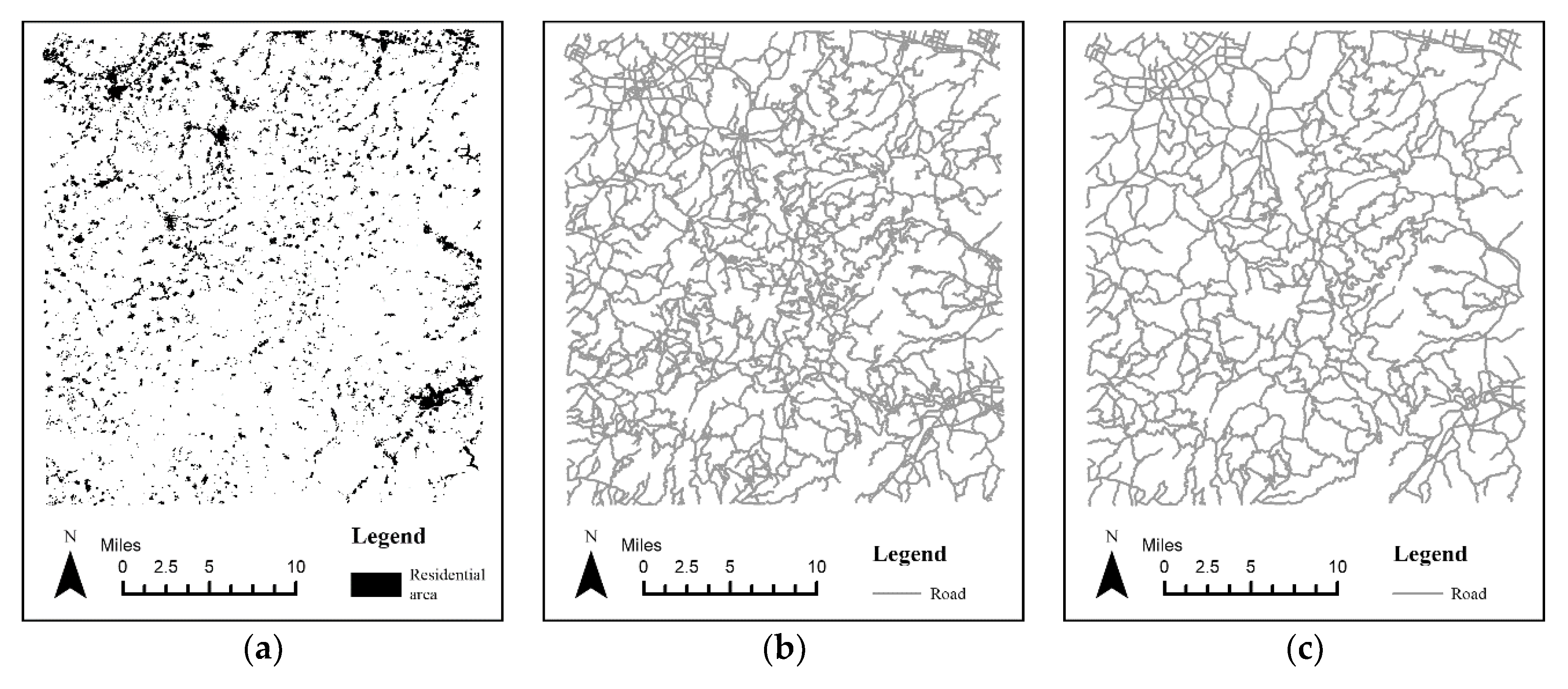
As presented in Figure 1, the 1:50,000 road network and residential area data around Ningbo City, Zhejiang Province, China were used as the experimental data, while an artificially produced 1:100,000 road network was used as the benchmark. The experimental area covered 1813 km2. There were 10,770 entities in the residential area data. The settlements were dominated by small-scale villages, with a few medium-scale towns and discrete buildings. There were 2750 roads in the road network, with a combined length of 2876.94 km. There were 1959 roads in the benchmark, with a combined length of 2181.62 km.
3.2. Framework
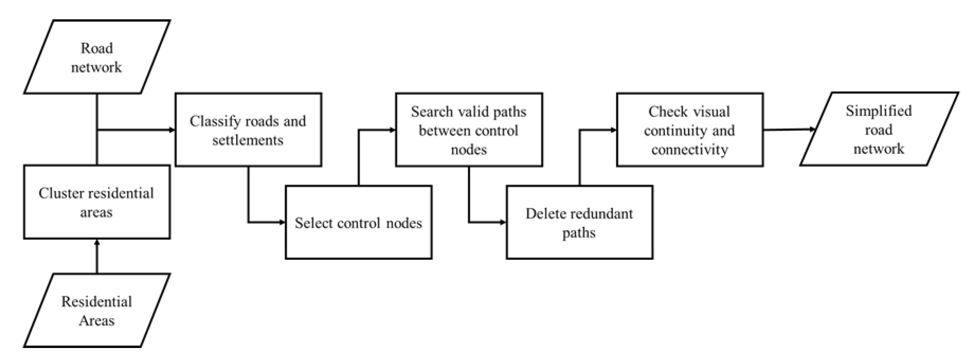
Our method aimed to constrain road network generalization by residential area to preserve the spatial distribution consistency and geographic correlation. This included the form of the road network, relative density characteristics, connectivity between settlements, and traffic efficiency. The settlements were used as the control features to decompose the complex road network generalization into relatively simple redundant paths between settlements. Figure 2 shows this method, which consisted of six basic steps:
- Cluster residential areas into settlements.
- Classify roads and settlements according to the topological relationship.
- Evaluate the importance of settlements and select certain settlements as control features.
- Build a geographic network with residential area and road network as nodes and edges, respectively, and search for the paths between settlements.
- Delete redundant paths between settlements.
- Check visual continuity and topological connectivity.
3.3. Classifying Roads and Settlements
First, it was necessary to cluster the residential areas. For residential areas, density-based clustering methods are commonly used. For this study, the classic density-based spatial clustering of applications with noise (DBSCAN) algorithm [25] was used to cluster the residential areas. The rolling circle method [26] was used to extract the outline of the settlements.
In order to facilitate the subsequent construction of the geographical network and path search, roads and settlements needed to be classified. As presented in Table 1, according to the topological relationship between roads and settlements, roads can be divided into extending roads (E-Roads), passing roads (P-Roads), inner roads (I-Roads), and outer roads (O-Roads).
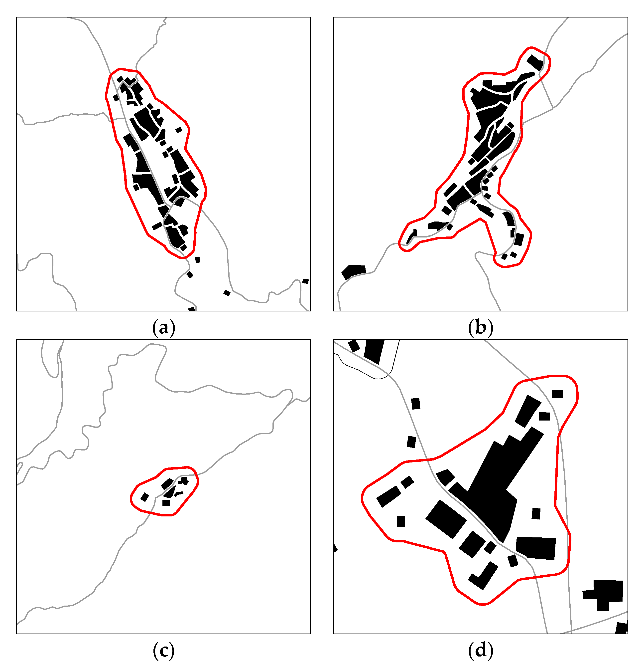
Settlements can be divided into two categories, according to the road type. Type I settlements mainly include E-Roads and I-Roads, or only E-Roads. Figure 3a shows an ideal and typical settlement. We followed the principle of “must have access to the core of the settlement.” Alternatively stated, the target road can only directly serve the settlement when it intersects with other roads within the settlement, or its range of influence covers the core of the settlement. The P-Road associated with the type I settlement shown in Figure 3b is an O-Road because it cannot directly serve the settlement. Type II settlements contain only P-Roads. As presented in Figure 3c, P-Roads, upon which settlements are completely dependent, penetrate most type II settlements. As shown in Figure 3d, some type II settlements contain multiple P-Roads. When evaluating which P-Roads are effective, we also followed the principle of “must have access to the core of the settlement.”
3.4. Evaluating Settlement Importance
As the service objects of road networks, residential areas have an important influence on the shape and structure of road networks. Compared with roads, residential areas have a higher priority, such that residential area generalization must be implemented first. Residential area generalization is also an important research topic in cartographic generalization, including selection, merging, and simplification. However, our focus was on road network generalization under the constraint of residential areas. Therefore, only some settlements were selected as the constraint conditions; no more steps were performed in residential areas. The importance of a settlement is usually evaluated in terms of semantic attributes, geometric characteristics, and location characteristics. Location characteristics refer to the positional relationships between settlements and roads. Hence, our method used the area (S), residential density (RD), Voronoi area (VS), and road index (RI) to evaluate the importance of settlements. A settlement set, i.e., , has the following information:
- S is the most intuitive embodiment of the importance of settlements. Generally, settlements with large areas are more important than those with small areas.
- RD reflects the density of residential areas within the settlement. When considering settlements with equal areas, settlements with more dense residential areas are more important. The RD was calculated as follows:where n is the number of residential areas in and denotes the residential area in .
- VS reflects the spatial influence of the settlement. The larger the Voronoi area, the more representative the settlement and the greater the possibility of its being selected.
- RI reflects the connectivity of the settlement. Settlement importance is affected by the number and grade of roads. The more roads associated with a settlement, and the higher the road grade, the higher the importance of the settlement. Settlements primarily rely on E- and P-Roads to connect their interiors to distant locations. For this reason, the RI is calculated based on the number and grade of the E- and P-Roads. The RI was calculated as follows:
These measured values were normalized such that all of the values ranged from 0–1. Hence, we used an integrated indicator (SP) to evaluate the relative importance of settlements as follows:
where is an adjustment factor. When S, RD, and VS are constant, settlements located at road intersections have more geographical significance than settlements distributed along roads. Therefore, when the evaluation object is a type I settlement, . When the evaluation object is a type II settlement, . The variables , , , and are the weights of S, RD, VS, and RI, respectively, and . These four weights and can be adjusted according to the requirements of the applications.
After the settlement importance evaluation was completed, some unqualified settlements were eliminated, according to the given rate threshold . All subsequent operations were based on settlements composed of the preserved settlements.
3.5. Searching Valid Paths
In a previous study, settlements were constructed and selected individually, rather than as parts of a neural network. The key to geographical networks is the proximity and connection between settlements. Cartographic generalization research usually uses the spatial distance, Delaunay triangulation, and Voronoi diagrams to express the spatial proximity relationships between geographical entities [27]. However, the spatial proximity relationship cannot effectively express the connected relationships of settlements in the road network. The effective path between settlements includes both direct and indirect connection paths. The entire direct connection path process involves only the start and end settlements, whereas the indirect connection path passes through other settlements in addition to the start and end settlements. If there is a direct connection path between two settlements, the two settlements are adjacent to each other along the road network.
The effective paths between settlements have two characteristics. (1) They connect from the E-Road of the beginning settlement to the end of the E-Road within the terminal settlement. Other E- and I-Roads in the beginning and ending settlements cannot be part of the path. The P-Road in the type II settlement, which effectively connects the interiors of two settlements, is an E-Road in the settlement. (2) The effective path is the least-cost path between the two E-Roads. This is because searching all of the paths between two nodes in a large network is time-consuming; people usually choose the shortest and fastest path when traveling. When planning a route, people pay more attention to time than distance, and tend to choose faster, high-grade roads. Therefore, travel time was used to express the cost. The travel time was primarily determined by the road length, road grade, and road tortuosity, as follows:
where L is the length, V is the road design speed, and ST is the tortuosity.
The connection between settlements refers to all of the effective paths between settlements. A settlement may have multiple E-Roads beginning at varying locations within the settlement. Therefore, there may be multiple paths between a pair of settlements. When searching for an effective path between a pair of adjacent settlements, the E-Road of the start settlement and the E-Road of the end settlement are arranged and combined. The Dijkstra algorithm [28] was used to search for the least-cost path between all the E-Road pairs and record the most effective path based upon that requirement.
3.6. Simplifying Redundant Paths
The redundant paths simplification of a geographical network can be divided into the following two stages: path simplification of adjacent settlement pairs and path simplification of adjacent settlement groups. Generally, a path with a lower cost is more preservation-worthy. However, preservation also depends on whether the services it provides can be replaced.
In the first stage, direct connection paths between adjacent settlements were evaluated. When simplifying the path between a pair of adjacent settlements, we chose any path to compare with the optimal path. If the cost of the path was greater than the sum of the optimal path and the internal traffic costs, the path was substituted. This rule was defined as follows:
where is the cost of the optimal path, is the internal travel cost of the optimal path and the current path in the start settlement, is the internal travel cost of the optimal path and the current path in the end settlement, is the cost of the current path, and is the tolerable cost ratio, i.e., the service capacity of the optimal path in the target area is weaker than the current path ( ranges from 0–1).
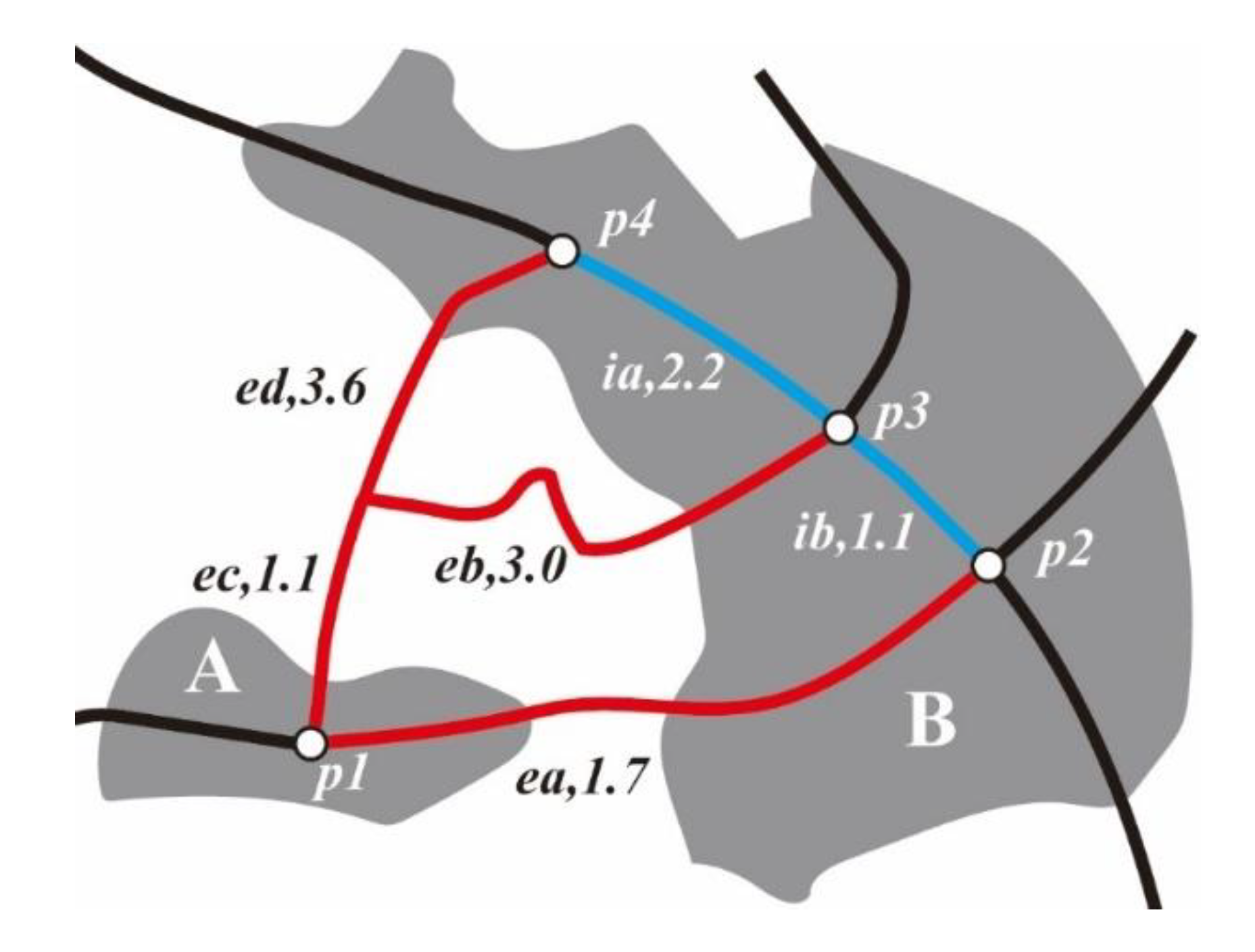
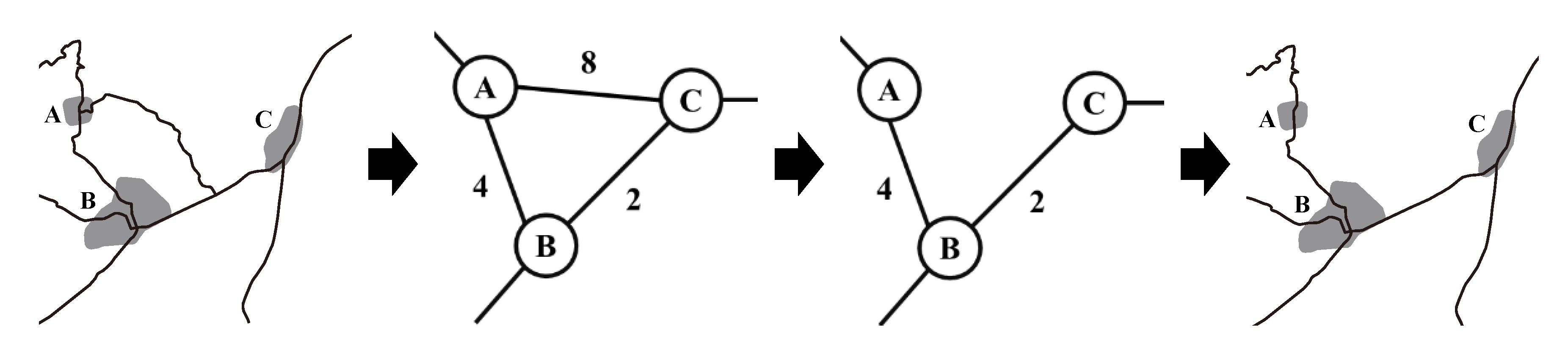
As presented in Figure 4, there are three paths between settlements A and B. Path I begins at point p1 and extends along ea to point p2. Path II begins at point p1 and extends along ec and eb to point p3. Path III begins at point p1 and extends along ec and ed to point p4. Path I is the optimal path. The start and end points of path II are p1 and p3, respectively, and the travel cost is 4.1. However, the total cost of traveling from p1 along path I to p2 and then along internal road ib to p3 is 2.8. This is less than the cost of path II, such that path II can be replaced by path I. Decreasing the value of can increase the intensity of simplification. For example, the cost of path III is 4.7. However, the total cost of traveling from p1 along path I to p2 and then along internal roads ib and ia to p4 is 5.0. When , Equation (5) does not work and path I cannot replace path III. However, when , Equation (5) is workable and path I can replace path III.
In the second stage, the proximity relationships between adjacent settlements are examined. All of the direct connection paths between adjacent settlements were treated as a whole, whose flow is shown in Figure 5. First, we constructed a graph with settlements and proximity relations as the nodes and edges, respectively, using the minimum cost of the direct connection paths between adjacent settlements as the edge weights. Next, we searched for the triangular structures in the graph, which were subgraphs composed of three adjacent settlements. Finally, we determined whether the edge with the largest weight in the triangular structure could be replaced by a combination of the other two edges. If so, all of the direct connection paths between the settlements connected by that edge were removed. This rule was defined as follows:
where is the tolerable cost ratio, is the maximum weight value in the subgraph, and and are the weight values of the two other edges.
After the path simplification was completed, some additional roads were selected to supplement the results and check the connectivity. The roads to be supplemented were I-Roads and visually continuous roads. The method of selection for the I-Roads was different from the selection of roads between settlements. The larger the settlement, the more complicated the process. The focus of our method was the selection of roads between settlements, such that only the lowest-cost path that could satisfy the connectivity of the preserved E-Roads within the settlements was selected. Other roads were supplemented based upon visual continuity. Some roads lacked connectable settlements at one end, but were supplemented because they had good visual continuity with preserved roads. Another criterion for selecting a supplemented road was that the preserved road had no other visually continuous roads at the intersection.
4. Results and Discussion
4.1. Determination of Thresholds
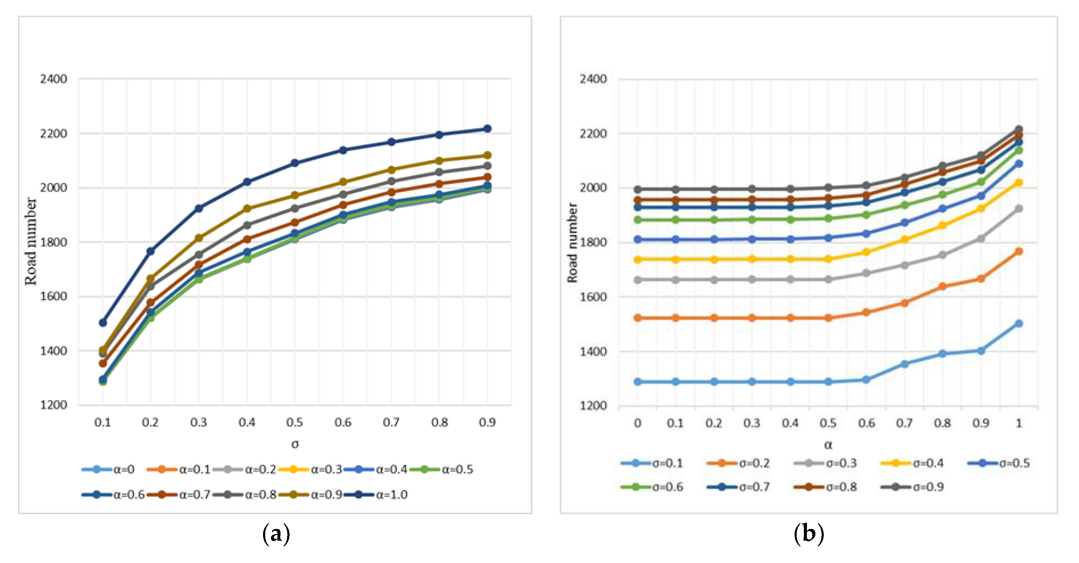
The quantity and quality of the results were affected by many factors, including the clustering quality, settlement selection ratio, angle threshold for evaluating visual continuity, and tolerable cost ratio. The most strongly influential factors were the settlement selection ratio () and the tolerable cost ratio (). The number of roads in the road network generated by the method was recorded under different parameter values (Table 2). The data were visualized and the influence of and on the number of roads was analyzed (Figure 6). The analysis showed that played a leading role in the selection and played an auxiliary adjustment role, which corresponds to the concept that settlements constrain the road network generalization.
The tolerable cost ratio () has limited adjustments. With respect to the experimental data, when the value of is fixed, the difference between the maximum and minimum values of the number of roads did not exceed 20%. The smaller the , the stronger the influence of and the greater the difference between the extreme values of the number of roads. As the number of settlements decreased, there were more direct connection paths between settlements and more paths became redundant. In addition, when was reduced to approximately 0.5, the maximum generalization intensity was reached. There was only one direct connection path between a pair of settlements and all the triangular structures on the graph were processed. Smaller values no longer affected the results. When , different values could effectively adjust the number of roads, which could be flexibly determined according to the value of and the expected number.
The selection ratio of the roads and settlements should be the same for cartographic generalization. The analysis shows that the number of roads was relatively close to the ideal value when . The smaller the value of , the greater the difference between the number of roads and the ideal value, indicating that our method is not suitable for road network generalization on a large scale because it is strongly influenced by residential areas. Road network and residential area generalization must be alternately implemented. Residential area generalization includes selection, merging, and simplification. Selecting settlements only on a large scale while skipping the other steps is unreasonable. With the continuous generalization of roads and residential areas, the role of a particular settlement or road changes dynamically. Two E-Roads may merge into a P-Road, type I settlements may become type II settlements, and multiple adjacent settlements may merge into one settlement.
In addition, supplementing visually continuous roads also affects the number of roads, where the degree of impact varies depending on the dataset. To achieve the expected generalization, when applying the SSP method to other datasets, multiple experiments must be implemented on different parameter combinations, according to the target scale. For our data set and target scale, we set and as 0.7 and 0.6, respectively.
4.2. Road Network Structure Analysis
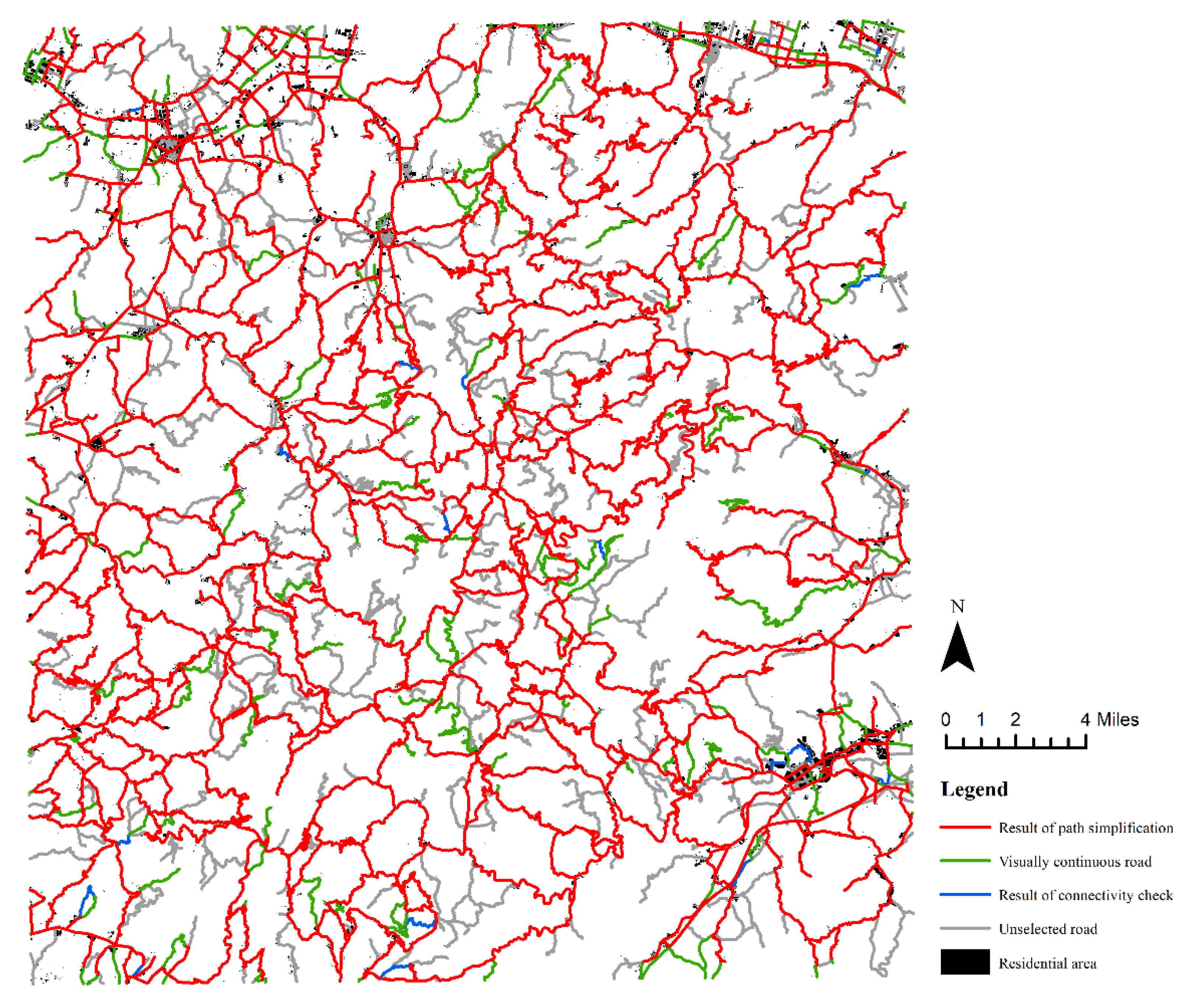
The target scale was 1:100,000 and 70% of the roads and settlements were selected, according to the law of the open square root model. With 594 settlements as constraints, 1948 roads were selected, of which 1613 roads were preserved in the path simplification stage. Next, 306 visually continuous roads were supplemented, along with 29 roads supplemented during the connectivity check. Through visual inspection, we determined that the overall structure and relative density characteristics of the road network were well maintained and in good agreement with the spatial distribution of the settlements. As presented in Figure 7, the red lines were the result of path simplification, which was highly consistent with the spatial distribution of the residential areas and could meet the connectivity needs of the settlements. The green lines were visually continuous roads supplemented by the principle of good continuity. The added roads were mainly located at abrupt road turning points and at the ends of roads in the road network of the previous stage.
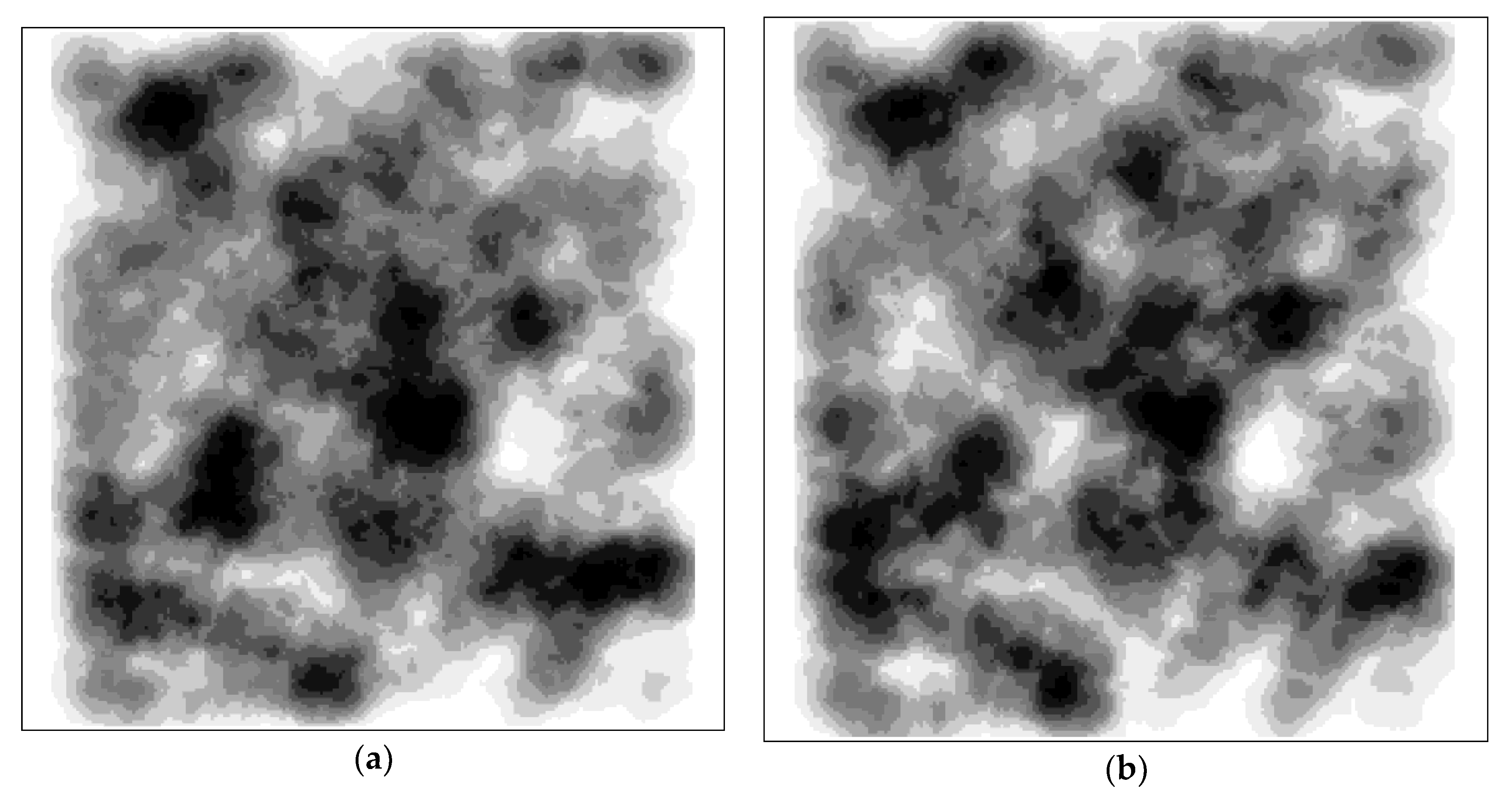
We performed a line density analysis on the road network before and after generalization. As presented in Figure 8, each density was divided into 10 sections and the relative density gradually increased (darkened) from low to high. After generalization, the high-density area of the road network was reduced, but the spatial distribution characteristics of the distinct density areas were comparable to those prior to the generalization. Areas with notable changes in the relative density were primarily concentrated in urban areas and sparse residential areas. The selection of I-Roads in towns was limited to those that represented the smallest sections that met the connectivity requirements. Sparse residential areas resulted in some roads being evaluated as having no connectivity values.
4.3. Geographical Correlation Analysis
Our method focuses most on the functionality and geographical correlation of the generalized road network. As presented in Figure 9, the generalized road network is in good agreement with the residential areas as the control features on the 1:100,000 map. The two features are highly consistent in spatial distribution. Most settlements are connected by roads. At the same time, redundant paths and a large number of suspended roads were deleted. A small number of settlements are not directly connected by roads because they are not within the specified road service range on the original scale.
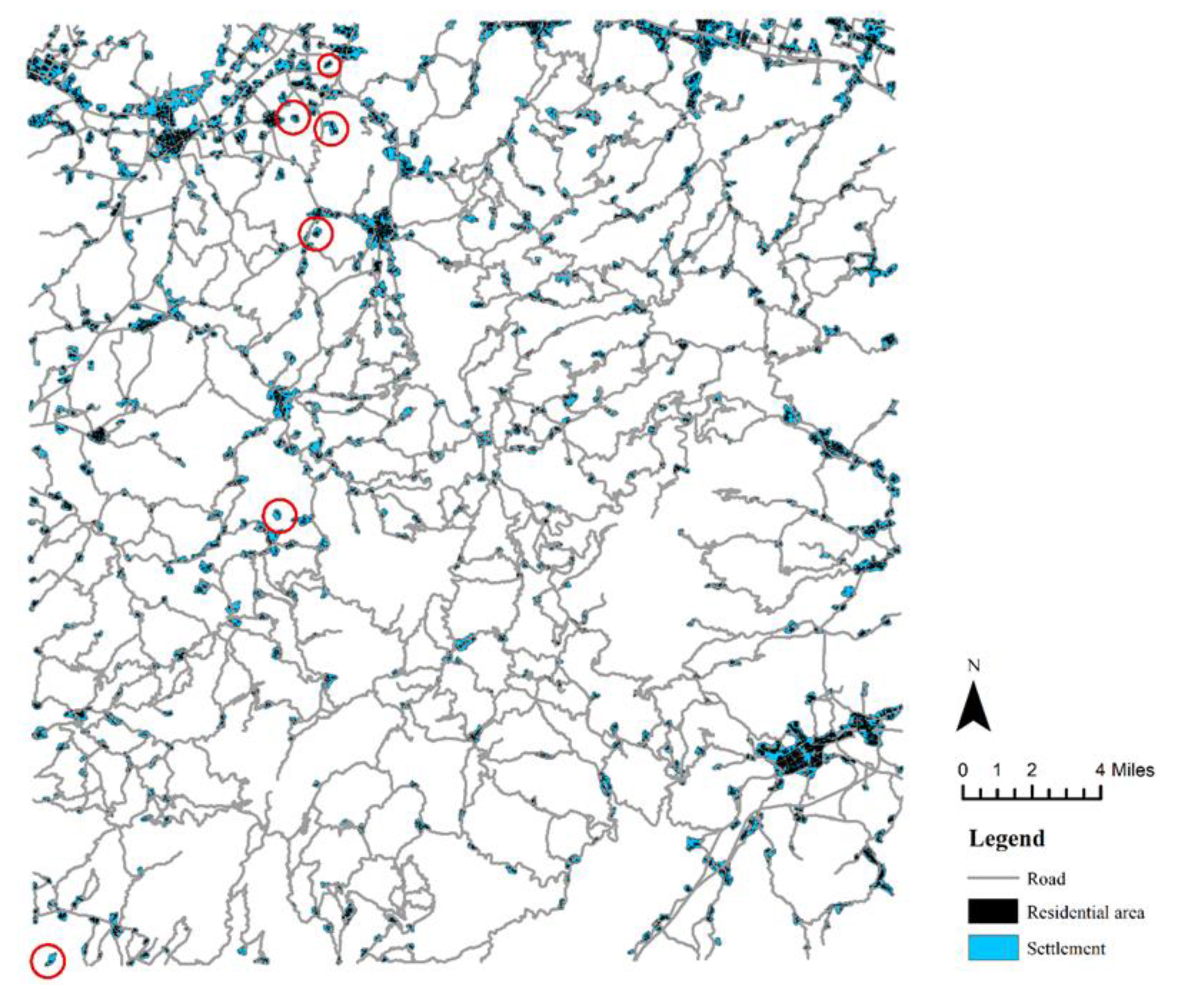
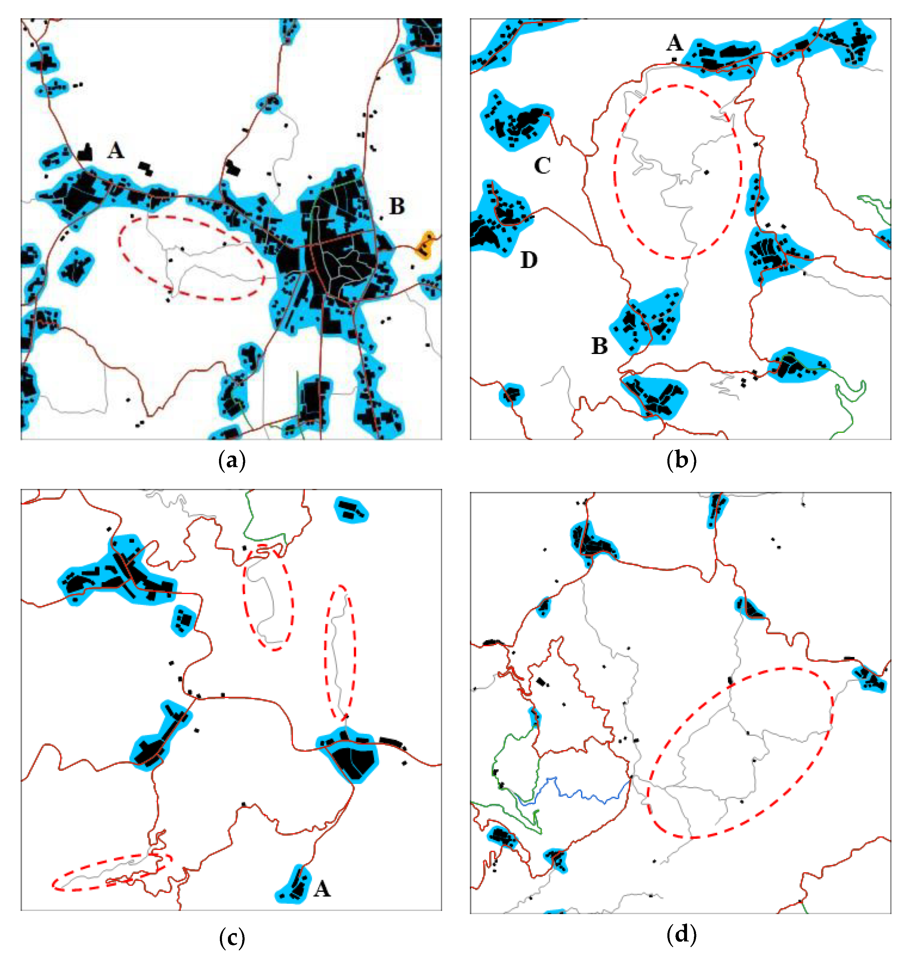
While maintaining geographical correlation, the redundant paths between settlements were also effectively simplified. In Figure 10a, there are three direct connection paths between the eastern and western settlements, including the main road and two partially overlapping trails. The two trails were removed because they could be replaced by the main road. In Figure 10b, there are three direct connection paths between the southern and northern settlements. The cost of the two gray roads in the middle was low, but they could only serve the start and end settlements. Although the path in the west was expensive, it was preserved because it was necessary for connecting the two western settlements with the other settlements. Figure 10c shows four suspended roads. The road connected with the settlement at the end was preserved, while the others were deleted. Therefore, the road network was generalized without damaging the connectivity of the settlements. However, our method performed poorly in sparse residential areas. In Figure 10d, gray roads are low in grade and weak in functionality, but they have an important impact on visual perception. Our method was not suitable for handling this type of road and requires further improvement.
4.4. Comparison with Other Methods
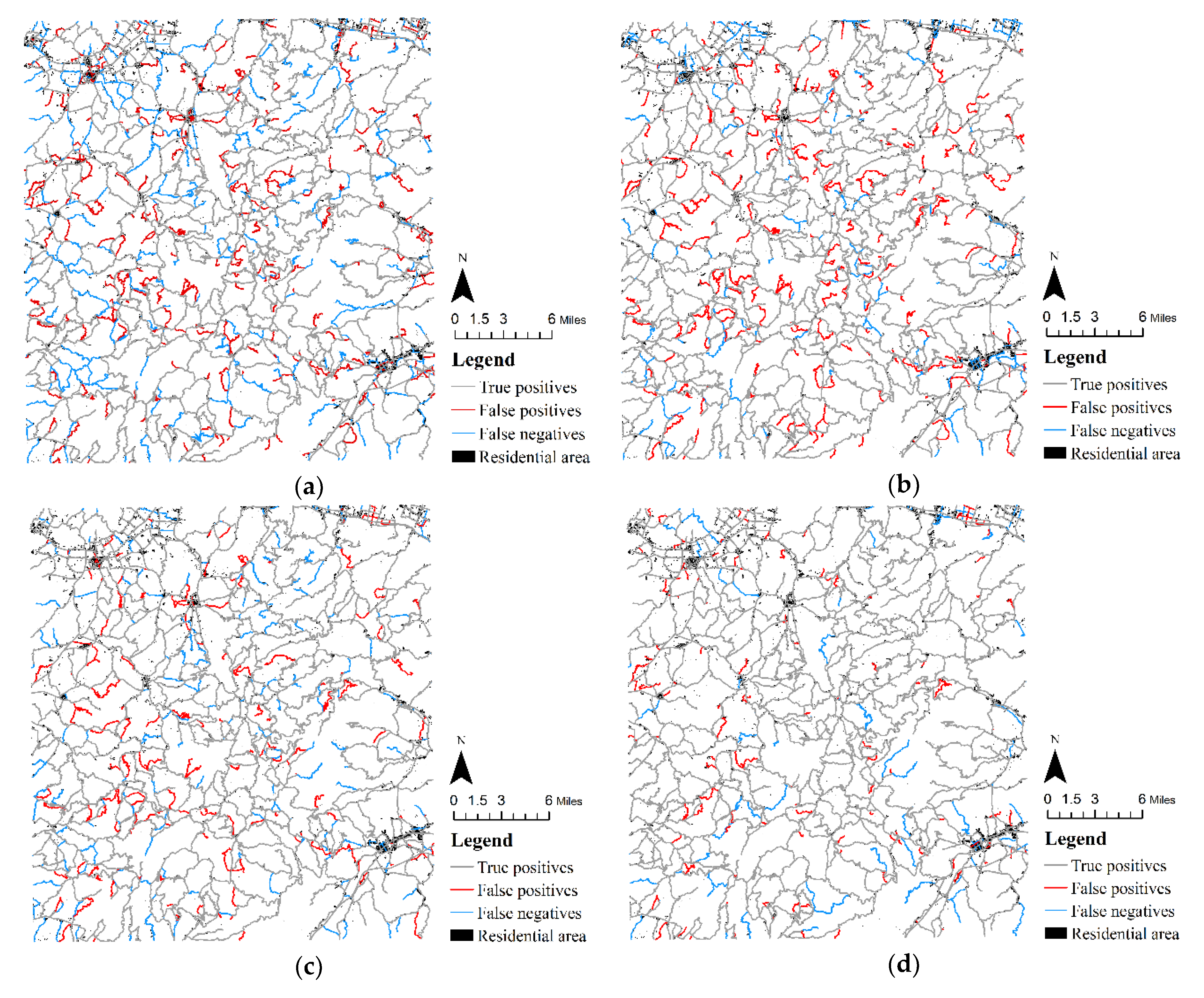
In order to further verify the effectiveness of this method, taking the artificially produced 1:100,000 road network as the benchmark, this method was compared with the graph-based method, stroke-based method, and hybrid method combining graph and stroke. In Figure 11a, the graph-based method uses the PageRank algorithm to evaluate the importance of road sections, without considering the topological information and geometrical information of the road network, resulting in poor visual continuity in the selection results. In Figure 11b, stroke-based uses length and road grade to evaluate the importance of stroke. The overall visual continuity is good, but there is a large number of redundant roads. In Figure 11c, the hybrid method takes into account the advantages of graph and stroke, and comprehensively evaluates the importance of stroke by using parameters such as length, grade, degree, closeness, and betweenness. The selection effect is significantly improved, but some settlements cannot be effectively connected. In Figure 11d, the results of our method are significantly better than those of the other methods. The missed components were mainly long-suspended roads that did not end at settlements and low-grade roads in sparsely populated areas. These had an impact on visual perception, but did not affect the functionality of the road network. The extra components mainly consisted of short suspension roads connecting the settlements and some visually continuous roads. Short suspension roads were selected because the algorithm could not fully simulate human spatial perception when evaluating the service between roads and settlements. When selecting visually continuous roads, the self-best-fit stroke generation method was used. This method determined whether two roads were visually continuous based on the angle at the intersection. This method cannot consider the overall performance of roads. Therefore, although it can improve the visual effect, it reintroduces some redundant roads with poor global performance. In general, the results of this method were closer to the artificially produced results; the method has significant advantages for maintaining the structural characteristics and geographical correlation of road networks.
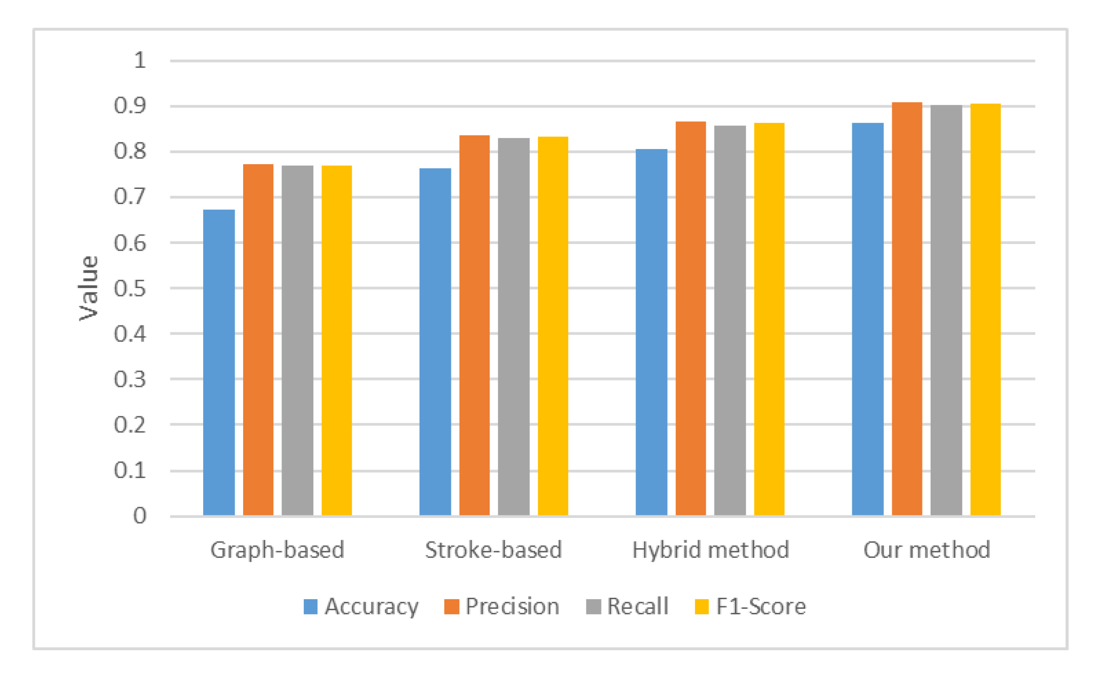
Further, the results were evaluated quantitatively. First, the consistency between the selection results and the benchmark was evaluated, and accuracy, precision, recall, and F1-Score were selected as the evaluation parameters. As presented in Figure 12, our method has the highest consistency with the benchmark (with accuracy, precision, recall, and F1-Score of 0.864, 0.907, 0.902, and 0.905, respectively), the closest relation to the artificially produced results, and the lowest difficulty and workload of subsequent processing.
In terms of geographical correlation, the global efficiency [29] and settlement coverage were used as evaluation parameters. The calculation object of global efficiency is the geographical network with settlements as nodes. Global efficiency reflects the traffic efficiency between the settlements in a network. It is defined as follows.
where N is the number of selected settlements and is the path cost from settlement i to settlement j.
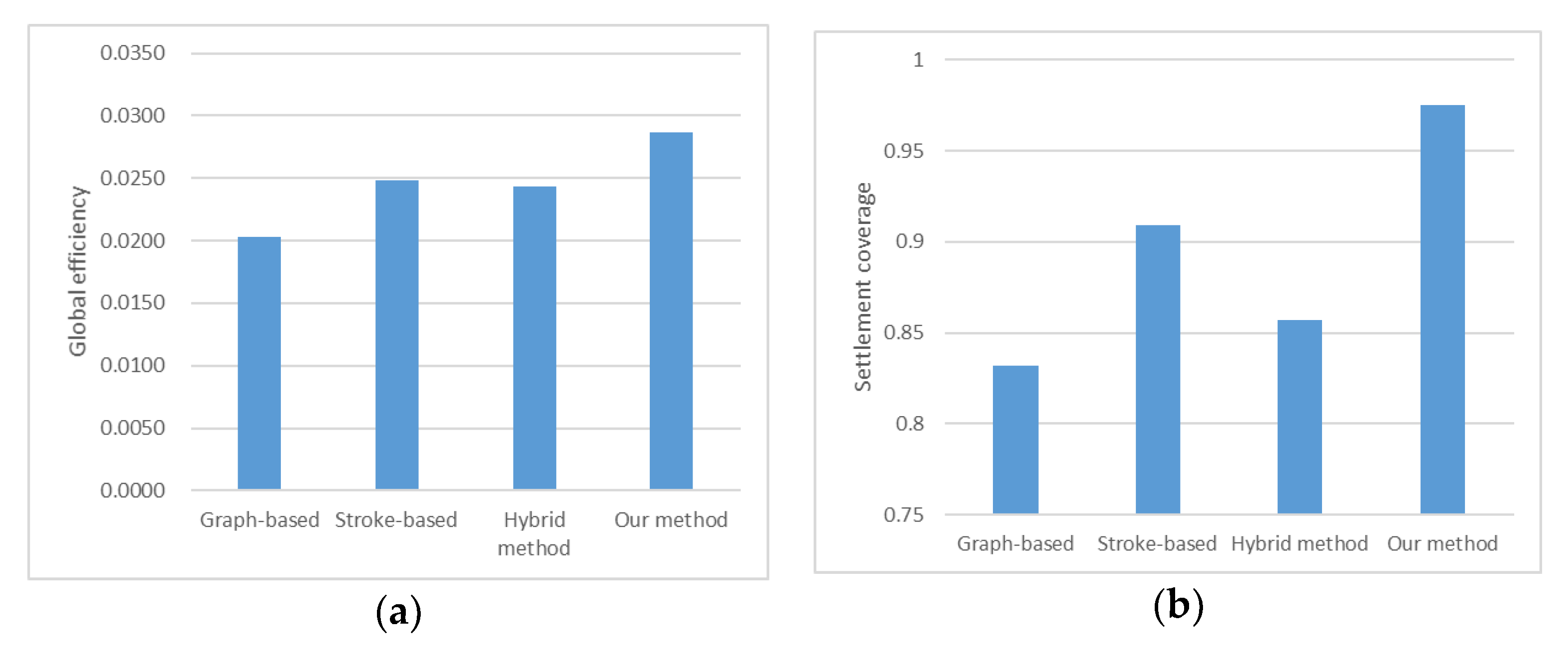
As presented in Figure 13, our method has the best traffic efficiency, the largest number of connected settlements, and the best geographical correlation between road networks and residential areas. Other methods do not take into account residential areas in the generalization, so their performance of geographical correlation is random. For example, although the hybrid method has high consistency with the benchmark, it is not as good as the stroke-based method in terms of geographical correlation.
5. Conclusions
Residential area and road network are a pair of map features with strong geographical correlation. When mapping, we should maintain their unique spatial distribution characteristics and geographical correlation between features. In this study, in order to ensure that the road network is in good agreement with residential areas, we propose a road network generalization method that is constrained by residential areas, which adopts the idea of divide-and-conquer, decomposes the road network with the settlements, and simplifies the complex road selection problem into a redundant path simplification problem. First, the roads and settlements obtained from residential clustering were classified. Subsequently, the importance of the settlements was evaluated and certain settlements were selected as the control features. Next, a geographical network with settlements as nodes was built. Finally, the redundant paths between settlements were deleted, and the visual continuity and topological connectivity were checked. This method makes full use of the geographical correlation of the two features. Using settlements as the constraint of road network generalization, the results were highly consistent with the spatial distribution of residential areas, which can ensure the connectivity between settlements and the functionality of road network.
In addition to the theoretical discussion, we also conducted empirical research. The experimental area was near Ningbo City, Zhejiang Province, China. The 1:50,000 road network and residential area data were used as the experimental data, while an artificially produced 1:100,000 road network was used as the benchmark. The experimental results show that this method performs well in terms of maintaining the spatial structure, density, and geographical correlation of road networks. Compared with the graph-based, stroke-based, and hybrid methods, the accuracy, precision, recall, and F1-Score of our method were as high as 0.864, 0.907, 0.902, and 0.905, respectively. The global efficiency and settlement coverage of our method were also better than other methods. The results showed that our method has significant advantages in the consistency of its benchmarking and geographical correlation with residential areas.
However, this study has some limitations. First, the proposed method represents only half of the full collaborative generalization method of the road network and residential area. Because it is incomplete, the proposed method is only suitable for road network generalization on a small scale. The complete method includes the residential area generalization method, considering the road network. Second, the proposed method highly depends on the spatial distribution of residential areas, and the effect is not good in areas with low residential density. To address this in the future, it will be necessary to identify and select additional roads in this type of area. Finally, the proposed method is not sufficiently automatic. To address this, it will be necessary to combine the data for multiple attempts to determine the parameter value. Road networks and geographical networks with settlements as nodes are typical complex-network structures, which are in good agreement with emerging graph neural networks. In the future, the collaborative generalization of roads and residential areas based on graph neural networks will be studied to improve the automation level of the algorithm.
Author Contributions
Conceptualization, Zheng Lyu; methodology, Zheng Lyu, Qun Sun, and Jingzhen Ma; software, Fubing Zhang; validation, Yuanfu Li; formal analysis, Zheng Lyu; investigation, Fubing Zhang; resources, Qun Sun; data curation, Yuanfu Li; writing—original draft preparation, Zheng Lyu.; writing—review and editing, Zheng Lyu, Jingzhen Ma, and Qing Xu; visualization, Zheng Lyu; supervision, Qun Sun; project administration, Qing Xu; funding acquisition, Qun Sun. All authors have read and agreed to the published version of the manuscript.
Funding
This study was supported by the National Natural Science Foundation of China (41571399, 42101458, 42101454, 42101455) and the Fund Project of Zhongyuan Scholar of Henan Province (202101510001).
Institutional Review Board Statement
Not applicable.
Informed Consent Statement
Not applicable.
Data Availability Statement
The data and codes that support the findings of this study are available at figshare.com with the following links: https://0-doi-org.brum.beds.ac.uk/10.6084/m9.figshare.17163533 (data, accessed on 12 December 2021) and https://0-doi-org.brum.beds.ac.uk/10.6084/m9.figshare.17163539 (code, accessed on 12 December 2021).
Acknowledgments
The authors are grateful to the editors and the anonymous referees for their valuable comments and suggestions.
Conflicts of Interest
The authors declare no conflict of interest.
References
- Wang, J.; Wu, F. Advances in Cartography and Geographic Information Engineering, 1st ed.; Springer: Singapore, 2021; pp. 151–211. ISBN 978-981-16-0613-7. [Google Scholar]
- Wu, F.; Gong, X.; Du, J. Overview of the Research Progress in Automated Map Generalization. Acta Geod. Cartogr. Sin. 2017, 46, 1645–1664. [Google Scholar] [CrossRef]
- Steiniger, S.; Weibel, R. Relations among Map Objects in Cartographic Generalization. Cartogr. Geogr. Inf. Sci. 2007, 34, 175–197. [Google Scholar] [CrossRef]
- Wang, C.; Wang, W.; Zhang, M.; Cheng, J. Evolution, Accessibility of Road Networks in China and Dynamics: From a Long Perspective. Acta Geogr. Sin. 2014, 69, 1496–1509. [Google Scholar] [CrossRef]
- Zhou, Y.; Huang, H.; Liu, Y. The Spatial Distribution Characteristics and Influencing Factors of Chinese Villages. Acta Geogr. Sin. 2020, 75, 2206–2223. [Google Scholar] [CrossRef]
- Gong, X. Research on Settlement Generalization Methods Considering Spatial Pattern and Road Networks. Ph.D. Thesis, PLA Strategic Support Force Information Engineering University, Zhengzhou, China, 2017. [Google Scholar]
- Li, G.; Xu, W.; Long, Y.; Zhou, T.; Gao, C. A Multi-constraints Displacement Method for Solving Spatial Conflict between Contours and Rivers. Acta Geod. Cartogr. Sin. 2014, 43, 1204–1210. [Google Scholar] [CrossRef]
- Šuba, R.; Meijers, M.; Oosterom, P.V. Continuous Road Network Generalization Throughout All Scales. ISPRS Int. J. Geo-Inf. 2016, 5, 145. [Google Scholar] [CrossRef] [Green Version]
- Mackaness, W.A.; Beard, K.M. Use of Graph Theory to Support Map Generalization. Cartogr. Geogr. Inf. Syst. 1993, 20, 210–221. [Google Scholar] [CrossRef]
- Liu, G.; Li, Y.; Yang, J.; Zhang, X. Auto-selection Method of Road Networks based on Evaluation of Node Importance for Complex Traffic Network. Acta Geod. Cartogr. Sin. 2014, 43, 97–104. [Google Scholar] [CrossRef]
- Jiang, B.; Harrie, L. Selection of Streets from a Network Using Self-organizing Maps. Trans. GIS 2004, 8, 335–350. [Google Scholar] [CrossRef]
- Ma, C.; Sun, Q.; Chen, H.; Xu, Q.; Wen, B. Application of Weighted PageRank Algorithm in Road Network Auto-selection. Geomat. Inf. Sci. Wuhan Univ. 2018, 43, 1159–1165. [Google Scholar] [CrossRef]
- Thomson, R.C.; Richardson, D.E. The Good Continuation Principle of Perceptual Organization Applied to the Generalization of road networks. In Proceedings of the 19th International Cartographic Conference, Ottawa, ON, Canada, 14–21 August 1999; pp. 1215–1223. [Google Scholar]
- Liu, X.; Zhan, F.; Ai, T. Road Selection Based on Voronoi Diagrams and “Strokes” in Map Generalization. Int. J. Appl. Earth Obs. Geoinf. 2010, 12, 194–202. [Google Scholar] [CrossRef]
- Cao, W.; Zhang, H.; He, J.; Lan, T. Road Selection Considering Structural and Geometric Properties. Geomat. Inf. Sci. Wuhan Univ. 2017, 42, 520–524. [Google Scholar] [CrossRef]
- Chen, J.; Hu, Y.; Li, Z.; Zhao, R.; Meng, L. Selective Omission of Road Features Based on Mesh Density for Automatic Map Generalization. Int. J. Geogr. Inf. Sci. 2009, 23, 1013–1032. [Google Scholar] [CrossRef]
- Li, Z.; Zhou, Q. Integration of Linear and Areal Hierarchies for Continuous Multi-Scale Representation of Road Networks. Int. J. Geogr. Inf. Sci. 2012, 26, 855–880. [Google Scholar] [CrossRef]
- Yu, W.; Zhang, Y.; Ai, T.; Guan, Q.; Chen, Z.; Li, H. Road Network Generalization Considering Traffic Flow Patterns. Int. J. Geogr. Inf. Sci. 2020, 34, 119–149. [Google Scholar] [CrossRef]
- Yamamoto, D.; Murase, M.; Takahashi, N. On-demand Generalization of Road Networks Based on Facility Search Results. IEICE Trans. Inf. Syst. 2019, 102, 93–103. [Google Scholar] [CrossRef]
- Guo, X.; Qian, H.; Wang, X.; Liu, J.; Zhong, J. A Method of Road Network Selection Based on Case and Ontology Reasoning. Acta Geod. Cartogr. Sin. 2021, 50, 1717–1727. [Google Scholar] [CrossRef]
- Zheng, J.; Gao, Z.; Ma, J.; Shen, J.; Zhang, K. Deep Graph Convolutional Networks for Accurate Automatic Road Network Selection. ISPRS Int. J. Geo-Inf. 2021, 10, 768. [Google Scholar] [CrossRef]
- Wei, Z.; He, J.; Wang, L. A Collaborative Displacement Approach for Spatial Conflicts in Urban Building Map Generalization. IEEE Access 2018, 6, 26918–26929. [Google Scholar] [CrossRef]
- Xu, W. Collaborative Map Generalization Method of Roads and Buildings Based on Multi-Agent. Master’s Thesis, Nanjing Normal University, Nanjing, China, 2014. [Google Scholar]
- Touya, G.A. Road Network Selection Process Based on Data Enrichment and Structure Detection. Trans. GIS 2010, 14, 595–614. [Google Scholar] [CrossRef] [Green Version]
- Ester, M.; Kriegel, H.P.; Sander, J.; Xu, X. A Density-Based Algorithm for Discovering Clusters in Large Spatial Databases with Noise. In Proceedings of the 2nd International Conference on Knowledge Discovery and Data Mining, Portland, OR, USA, 2–4 August 1996; pp. 226–231. [Google Scholar]
- Zhi, L.; Yu, X.; Li, G. Spatial Point Clustering Analysis Based on the Rolling Circle. Geomat. Inf. Sci. Wuhan Univ. 2018, 43, 1193–1198. [Google Scholar] [CrossRef]
- Brennan, J.; Martin, E. Spatial Proximity Is More than Just a Distance Measure. Int. J. Hum. Comput. Stud. 2012, 70, 88–106. [Google Scholar] [CrossRef]
- Makariye, N. Towards Shortest Path Computation Using Dijkstra Algorithm. In Proceedings of the 2017 International Conference on IoT and Application (ICIOT), Nagapattinam, India, 19–20 May 2017; pp. 1–3. [Google Scholar]
- Latora, V.; Marchiori, M. Efficient Behavior of Small-World Networks. Phys. Rev. Lett 2001, 87, 1–18. [Google Scholar] [CrossRef] [PubMed] [Green Version]
Figure 1.
Experimental and benchmark data: (a) 1:50,000 residential areas, (b) 1:50,000 road network, and (c) 1:100,000 road network.
Figure 1.
Experimental and benchmark data: (a) 1:50,000 residential areas, (b) 1:50,000 road network, and (c) 1:100,000 road network.

Figure 2.
Flow of the road network generalization method constrained by residential areas.

Figure 3.
Classification of settlements: (a) typical type I settlement; (b) type I settlement with P-Road; (c) typical type II settlement; and (d) type II settlement with multiple P-Roads.
Figure 3.
Classification of settlements: (a) typical type I settlement; (b) type I settlement with P-Road; (c) typical type II settlement; and (d) type II settlement with multiple P-Roads.

Figure 4.
Schematic diagram of the path simplification between settlements (red lines are paths between settlements A and B; blue lines are I-Roads).
Figure 4.
Schematic diagram of the path simplification between settlements (red lines are paths between settlements A and B; blue lines are I-Roads).

Figure 5.
Settlement group path simplification process.

Figure 6.
Number of selected roads under varying parameter values: (a) road number under varying values and (b) road number under varying values.
Figure 6.
Number of selected roads under varying parameter values: (a) road number under varying values and (b) road number under varying values.

Figure 7.
Results of generalization on a 1:100,000 scale (red lines are the results of path simplification, green lines are visually continuous roads, blue lines are the selected roads in the connectivity check, and gray lines are the unselected roads).
Figure 7.
Results of generalization on a 1:100,000 scale (red lines are the results of path simplification, green lines are visually continuous roads, blue lines are the selected roads in the connectivity check, and gray lines are the unselected roads).

Figure 8.
Comparison of the relative road density before and after generalization: (a) road density before generalization and (b) road density after generalization.
Figure 8.
Comparison of the relative road density before and after generalization: (a) road density before generalization and (b) road density after generalization.

Figure 9.
Generalized road network and residential areas in 1:100,000.

Figure 10.
Partial details of the results: (a–c) show the advantages of SSP and (d) shows the shortcomings of SSP.
Figure 10.
Partial details of the results: (a–c) show the advantages of SSP and (d) shows the shortcomings of SSP.

Figure 11.
Comparisons between the benchmark and four methods: (a) Comparison between the results of the graph-based method and benchmark. (b) Comparison between the results of the stroke-based method and benchmark. (c) Comparison between the results of the hybrid method and benchmark. (d) Comparison between the results of our method and benchmark.

Figure 12.
The consistency between results and benchmark.

Figure 13.
Performance of four methods in geographical correlation: (a) the global efficiency of the results; (b) the settlement coverage of the results.
Figure 13.
Performance of four methods in geographical correlation: (a) the global efficiency of the results; (b) the settlement coverage of the results.


Table 1.
Explanation of road types (examples are shown as red lines).
| Topological Characteristics | Example | Description | |
|---|---|---|---|
| E-Road | One end is located inside the settlement and the other end is located outside the settlement. |  | E-Roads directly connect the interior and exterior of the settlement, which represent the starting and ending sections of the path between settlements. |
| P-Road | Both ends are outside the settlement with a section passing through the settlement. |  | P-Roads can also connect the interiors and exteriors of settlements. They are common in small settlements distributed along roads and occasionally in larger settlements. |
| I-Road | Both ends are contained within the settlement. |  | The function of an I-Road is to connect E-Roads and different areas within the settlement. The larger the settlement, the greater the number of I-Roads and the more complex the structure. |
| O-Road | Completely outside the settlement. |  | O-Roads are separated from the target settlement and do not participate in the construction of settlements. |
Table 2.
Number of selected roads under varying and values.
| σ = 0.1 | σ = 0.2 | σ = 0.3 | σ = 0.4 | σ = 0.5 | σ = 0.6 | σ = 0.7 | σ = 0.8 | σ = 0.9 | |
|---|---|---|---|---|---|---|---|---|---|
| α = 0.0 | 1288 | 1523 | 1663 | 1738 | 1811 | 1883 | 1929 | 1957 | 1995 |
| α = 0.1 | 1288 | 1523 | 1663 | 1738 | 1811 | 1883 | 1929 | 1957 | 1995 |
| α = 0.2 | 1288 | 1523 | 1663 | 1738 | 1811 | 1883 | 1929 | 1957 | 1995 |
| α = 0.3 | 1288 | 1523 | 1664 | 1739 | 1812 | 1884 | 1930 | 1958 | 1996 |
| α = 0.4 | 1288 | 1523 | 1664 | 1739 | 1812 | 1884 | 1930 | 1958 | 1996 |
| α = 0.5 | 1288 | 1523 | 1664 | 1739 | 1817 | 1889 | 1935 | 1963 | 2001 |
| α = 0.6 | 1296 | 1543 | 1688 | 1765 | 1833 | 1902 | 1948 | 1975 | 2009 |
| α = 0.7 | 1354 | 1578 | 1717 | 1811 | 1873 | 1937 | 1984 | 2015 | 2039 |
| α = 0.8 | 1391 | 1639 | 1755 | 1863 | 1925 | 1976 | 2024 | 2058 | 2081 |
| α = 0.9 | 1403 | 1667 | 1815 | 1924 | 1972 | 2022 | 2067 | 2100 | 2120 |
| α = 0.10 | 1504 | 1768 | 1925 | 2021 | 2091 | 2139 | 2169 | 2195 | 2217 |
| Ideal value | 275 | 550 | 825 | 1100 | 1375 | 1650 | 1925 | 2200 | 2475 |
Publisher’s Note: MDPI stays neutral with regard to jurisdictional claims in published maps and institutional affiliations. |
© 2022 by the authors. Licensee MDPI, Basel, Switzerland. This article is an open access article distributed under the terms and conditions of the Creative Commons Attribution (CC BY) license (https://creativecommons.org/licenses/by/4.0/).
Share and Cite
MDPI and ACS Style
Lyu, Z.; Sun, Q.; Ma, J.; Xu, Q.; Li, Y.; Zhang, F. Road Network Generalization Method Constrained by Residential Areas. ISPRS Int. J. Geo-Inf. 2022, 11, 159. https://0-doi-org.brum.beds.ac.uk/10.3390/ijgi11030159
AMA Style
Lyu Z, Sun Q, Ma J, Xu Q, Li Y, Zhang F. Road Network Generalization Method Constrained by Residential Areas. ISPRS International Journal of Geo-Information. 2022; 11(3):159. https://0-doi-org.brum.beds.ac.uk/10.3390/ijgi11030159
Chicago/Turabian StyleLyu, Zheng, Qun Sun, Jingzhen Ma, Qing Xu, Yuanfu Li, and Fubing Zhang. 2022. "Road Network Generalization Method Constrained by Residential Areas" ISPRS International Journal of Geo-Information 11, no. 3: 159. https://0-doi-org.brum.beds.ac.uk/10.3390/ijgi11030159
Note that from the first issue of 2016, this journal uses article numbers instead of page numbers. See further details here.