Optimizing the Sampling Area across an Old-Growth Forest via UAV-Borne Laser Scanning, GNSS, and Radial Surveying

Abstract

Aboveground biomass, volume, and basal area are among the most important structural attributes in forestry. Direct measurements are cost-intensive and time-consuming, especially for old-growth forests exhibiting a complex structure over a rugged topography. We defined a methodology to optimize the plot size and the (total) sampling area, allowing for structural attributes with a tolerable error to be estimated. The plot size was assessed by analyzing the semivariogram of a CHM model derived via UAV laser scanning, while the sampling area was based on the calculation of the absolute relative error as a function of allometric relationships. The allometric relationships allowed the structural attributes from trees’ height to be derived. The validation was based on the positioning of a number of trees via total station and GNSS surveys. Since high trees occlude the GNSS signal transmission, a strategy to facilitate the positioning was to fix the solution using the GLONASS constellation alone (showing the highest visibility during the survey), and then using the GPS constellation to increase the position accuracy (up to PDOP~5−10). The tree heights estimated via UAV laser scanning were strongly correlated (r² = 0.98, RMSE = 2.80 m) with those measured in situ. Assuming a maximum absolute relative error in the estimation of the structural attribute (20% within this work), the proposed methodology allowed the portion of the forest surface (≤60%) to be sampled to be quantified to obtain a low average error in the calculation of the above mentioned structural attributes (≤13%).

1. Introduction

Most geomatic techniques (conventional traverse surveying and GNSS [1], LiDAR [2], photogrammetry [3], remote sensing [4], geographical information systems [5]) have been used, in recent years, to characterize forests’ and trees’ planimetric positions. In particular, the development of remote sensing technology in recent decades has been revolutionary for forestry applications (acronyms and symbols are reported in Appendix A).

The most significant progress is due to the introduction of airborne laser scanning (ALS) and recently of unmanned aerial vehicle-borne laser scanning (UAVLS) or unmanned laser scanning (ULS) [6]. ALS and UAVLS have been successfully used to measure tree height [7,8,9,10], and to estimate a wide range of canopy properties, including crown diameter [11], canopy structure [12], leaf area [13], canopy fuel [14], and canopy gaps [15]. Forest structural attributes such as basal area, volume, and aboveground biomass can be modelled or inferred from these direct measurements [16,17,18,19,20,21,22,23]. ALS has been widely investigated for applications in forest inventories [24,25,26,27,28]. Furthermore, the applicability of ALS for detecting characteristics such as structural attributes of old-growth forests is currently rapidly increasing [29,30,31,32]. Recent studies have strongly supported the conservation of old-growth forests as an effective global strategy to tackle observed and forecasted effects of climate change [33,34]. It is now well recognized that old-growth forests play an effective role in biodiversity conservation at the landscape and stand scales [35,36] and in ecosystem services provision such as carbon storage [37,38]. In the assessment of old-growth forests, the structural attributes are usually characterized in the field by sampling a number of plots [29,39,40,41]. The design of fixed-size plots, randomly or systematically located within the investigated area, is considered a consolidated and effective way to estimate ecological attributes [42]. Several studies have analyzed the effect of sample plot size on the estimation of forest structural attributes [22,43,44,45,46,47]. Plot size is a key sampling design parameter because it can reduce or inflate potential edge effects, influencing the accuracy of forest stand attributes [44]. Standard practice in establishing ALS-based models for estimating plot- or stand-level structural attributes often employs a two-stage sampling approach with in situ measurements frequently simultaneous with ALS acquisitions [48]. This two-stage procedure can be cost-intensive and time-consuming, especially in forests characterized by complex structure and topography. The topography often includes steep slopes, deep valleys, peaks, and rock outcrops. Typically, these conditions occur in Mediterranean old-growth forests located in remote and impervious mountain areas [49,50,51] characterized by low levels of accessibility. Our specific objectives were to implement a methodology (1) to determine a representative plot size, given the spatial variability of the heights of the trees, and (2) to estimate a sampling area allowing the structural attributes to be characterized with a satisfactory level of accuracy. Indeed, such a methodological approach is particularly important in surveying impervious areas characterized by a low accessibility level. Technically, it was necessary to deal with the limits of the GNSS positioning in mountain forested areas. We suggested a strategy to fix the initial solution based on the constellation of which the largest number of satellites is visible, regardless of which constellation they belong to.

2. Materials

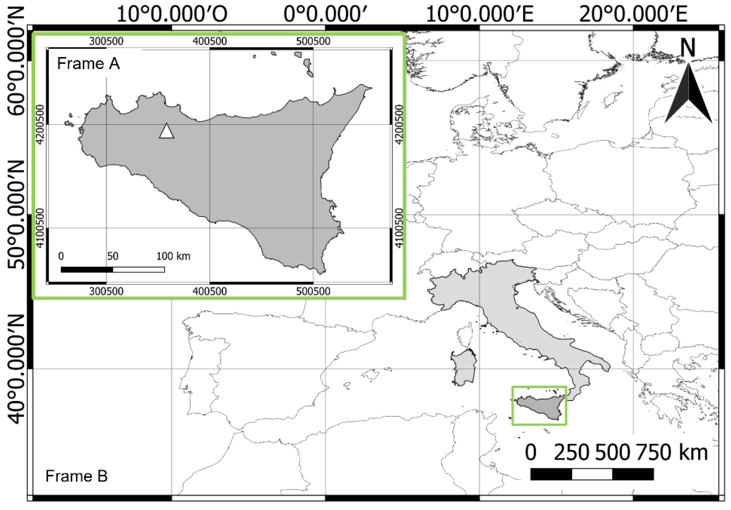
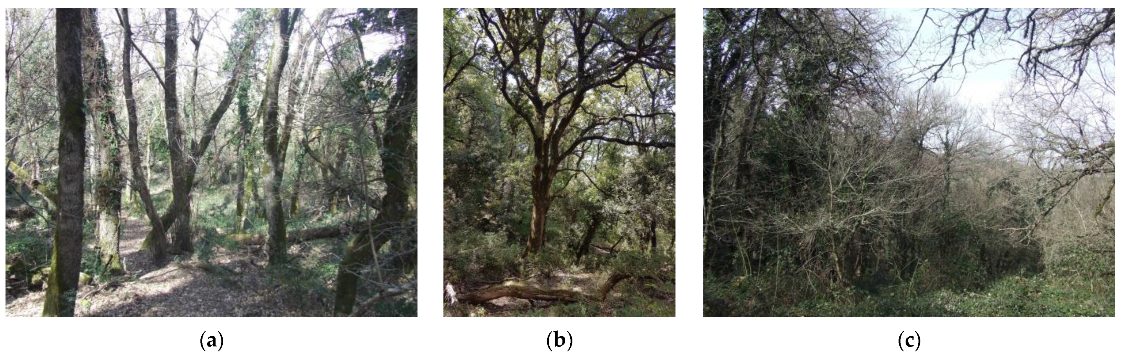
2.1. Study Area

The study was carried out in northwest Sicily (Italy) in an old-growth forest stand (37°51′29″ N, 13°25′42″ E) (Figure 1). The stand is located in a narrow valley at altitudes of 1000–1050 m, northwest exposed, within the “Bosco della Ficuzza, Rocca Busambra, Bosco del Cappelliere, Gorgo del Drago” Regional Nature Reserve, and part of the Special Areas of Conservation (SAC) “Monti Sicani, Rocca Busambra, Bosco della Ficuzza”. This latter is included in the Natura 2000 network (ITA020048, Habitat Directive 92/43/EC). The stand (~1.2 ha) is dominated by downy oak (Quercus pubescens Willd.) with other broadleaves such as holm oak (Quercus ilex L.), field maple (Acer campestre L.), and sweet chestnut (Castanea sativa Mill.). It has escaped natural and anthropogenic disturbances such as wildfires, harvesting, and gathering of deadwood for at least 80 years. During this period, the stand moved towards late-successional developmental stages with high levels of structural complexity, including a multi-layer canopy, canopy gaps created by tree mortality, large old trees, and accumulations of standing and lying deadwood [52]. The bioclimate is Mediterranean pluviseasonal–oceanic with mesomediterranean thermotype and subhumid ombrotype [53]. Soils can be classified as leptosols [54] (https://www.fao.org/3/i3794en/I3794en.pdf, accessed on 11 February 2022). According to the approach of forest accessibility [5], the study area was classified as barely accessible.

2.2. Forest Structural Attributes Data

A field survey was carried out in May 2016, on the old-growth forest stand, including large old trees, deadwood, lying and leaning trees, as well as canopy gaps (Figure 2). We measured the diameter at breast height (DBH, m) and height (H, m) of living trees. Field reference data were used to derive single-tree attributes such as basal area (G, m²), growing stock volume (V, m³), and aboveground biomass (AGB, Mg).

A total of 413 trees belonging to 11 species was censused, of which 100 were large old trees with DBH > 0.04 m. V, G, and AGB per hectare were estimated to be 293.5 m³, 27.8 m², and 227.2 Mg, respectively. Large old trees represented 71% of V, 60% of G, and 69% of AGB.

Note that in natural deciduous forests, such as our old-growth forest stand, the tree detection rate in situ is lowered by the dense canopy structure. In addition, the treetop often does not correspond to tree position at breast height. This is the case for irregular canopy shape and tree leanings (Figure 2a,b) from ALS data [55].

The ability of ALS to record suppressed and lying trees is limited by the uppermost canopy layer [10,21]. Moreover, the exact identification of treetop locations from the point clouds can be challenging for intermediate and suppressed trees, even with human inspections [10]. Therefore, suppressed trees were excluded from the following analyses. The resulting 276 trees, classified as the dominant, codominant, and intermediate crown, were used as reference field data and matched with ALS-detected trees.

2.3. UAV-Borne Laser Scanning Data

UAVLS data were acquired on 4 May 2016 under leaf-on conditions using a YellowScan Mapper, mounted on a remotely piloted aerial system, with the following technical specifications: 1.8 m-diameter octocopter, characterized by a Global Positioning System (GPS) waypoint navigation, auto take-off, and landing. The YellowScan Mapper is a class 1 laser working in the near-infrared (at 905 nm). The planimetric absolute accuracy of the integrated system is 0.10 m + 1% of the flying altitude, the vertical accuracy is 0.10 m + 0.5% of the acquisition altitude, while the precision is 10 cm. The range resolution is 4 cm. The LiDAR instrument was integrated with an internal inertial navigation system (INS) and GPS+ receiver (GPS plus GLONASS, Global’naja Navigacionnaja Sputnikovaja Sistema) acquiring in real-time kinematics (RTK). The system weight and autonomy were about 2 kg and 3 h, respectively [56]. The UAV operated up to 50 m above treetops, recording a maximum of three returns per laser pulse. The scan angle range was ±50°. The scanned area was composed of seven parallel and partly overlapping strips, acquired at a flight speed of ≈0.5 m/s, resulting in an acquisition duration of 35′. The strips were labelled as S1–S7 from north to south.

2.4. Topographic and Expeditious Surveys

The topographic phase consisted of a closed traverse of GNSS benchmarks together with a radial-line survey. A GNSS Topcon Hiper-Pro, both GPS and GLONASS, receiving in double-frequency and equipped with an FC-100 controller, was used for the static survey of two reference landmarks, while for the closed traverse survey, a Leica TPS 1105 total station (Hexagon AB, Sweden) and topographic right-angle prisms were employed. The system is characterized by an angle measurement accuracy of 3″ (1 mgon) and a distance measurement (Infrared sensor, IR) accuracy (ISO 17123-4) in standard mode of 2 mm.

The commercial software for the topographic geolocation of the trees was the following:

−

MAGNET Tools and Topcon Tools ver. 8.2.3, developed by Topcon Corporation (Tokyo, Japan). The software allows data processing from different devices such as total stations, digital levels, and GNSS receivers, and it is used in most technical–scientific applications [57,58,59]. Topcon Tools includes different models for tropospheric correction, such as the Modified Hopfield Model [60,61,62] with the NRLMSISE meteorological model, in extenso the United States Naval Research Laboratory Mass Spectrometer Incoherent Scatter Radar model [63]. Baseline processing can take place either with the GPS or GLONASS constellations or a combination of the two (GPS+).

−

Meridiana ver. 2020, developed by Geopro (Topcon Positioning Italy, Ancona, Italy). The tool allows the geographical congruence to be analyzed and outliers of the total station data to be checked, assuming a given set of tolerances. Depending on the data available, the software uses the following calculation methods: roto-translation (rigid or least-squares, with fixed or variable scaling factor), Snellius, and Ex-center.

−

The theoretical number of satellites, for the given cutoff angle, was calculated using the Trimble GNSS planning online software [64].

The expeditious phase consisted of some radial-line surveys using a hypsometer and a compass. Indeed, twelve additional reference landmarks were placed in the area, and their coordinates were determined using a Recon N324 GNSS receiver (by Trimble Inc., Sunnyvale, California, USA) (≈2 m accuracy in absolute method). The landmarks were placed on the boundary, both in the corners and in the midpoint of each side, as well as in the gaps occurring within the area. This allowed the maximum distance between the trees and the nearest landmark (≤30 m) to be limited. The coordinates of the living trees were determined by recording horizontal distance and azimuth readings for every tree from the nearest landmark, using the Vertex IV hypsometer (Haglöf, Långsele, Sweden) and the Tandem/360PC/360R DG Clino/Compass (Suunto, Vantaa, Finland). The accuracy of the hypsometer is <1% of the distance, while the precision of the compass is 20′.

3. Methods

3.1. Data Collection

The surveys consisted of the structural characterization of the forest, as well as the tree positioning.

The DBH and H of living trees >0.03 m were measured using a caliper (Silvanus type 1208) and a hypsometer, respectively [65]. We also classified the species and the tree crowns as dominant, codominant, intermediate, or suppressed [66]. Species-specific allometric equations were used to predict V and AGB [67], which combine DBH and H.

For the tree topographic positioning, the choice of a specific technique instead of another is dependent on various factors. Some limits can be overcome by integrating different geomatics techniques, for instance, the total station and GNSS surveys.

Indeed, while it is always possible to apply classical topographic approaches, such as conventional traverse (with total stations), according to Meyer et al. [68] the use of GNSS positioning is degraded by the influence of the canopy, which naturally obstructs the sky and reduces signal acquisition. Many factors are responsible for the decrease of accuracy in positioning of the forest trees, including multipath, cycle slip, low signal-to-noise ratio (SNR, −), and low dilution of precision (DOP, −).

The feasibility of surveying in GNSS kinematic mode was excluded, since even with the aid of micro-electro-mechanical systems (MEMS), it allows a horizontal accuracy not higher than 15–50 m to be achieved [69]. In addition, the poor GSM signal in the study area led to the discarding of the use of low-cost mobile phone sensors, although given the technological development of these sensors [70,71], their use is increasingly spreading. Since the planimetric positioning of the trees depends on the availability and quality of the GSM signal, the accuracies achieved by the authors are modest, in the range of 5–15 m. Fan et al. [72], on the other hand, by equipping the mobile phone with an additional Red Green Blue-Depth (RGB-D) MMS Simultaneous Localization and Mapping (SLAM), reported being able to position the trees with sub-meter accuracy.

Therefore, it was decided to survey some of the forest control points, according to [73,74], and, based on Valbuena et al. [75], a closed traverse survey of under canopy GNSS benchmarks with a radial-line survey was employed, allowing the axis of a number of trees to be positioned at breast height.

Regarding the differential correction of GNSS data, applications have benefited from Continuously Operating Reference Stations (CORS) for three-dimensional positioning. Scientific and technical applications of the CORS networks have been developed for real-time positioning (Network Real-Time Kinematic (NRTK)), as well as for data post-processing. Indeed, the GNSS CORS network allowed a reliable differential correction to be received using approaches such as the Virtual Reference Station (VRS), the Flächen-Korrektur-Parameter (FKP), or the Multi Reference Station (MRS).

The University of Palermo (UNIPA) materialized a GNSS CORS network in the western part of Sicily (Italy) providing daily data in Receiver Independent Exchange (RINEX) format (at 30″ rate) and hourly raw data (at 1″ rate); the network is made up of eight CORSs serving near 740,000 hectares, equipped with Topcon NET G-3 GPS and GLONASS enabled receivers [76]. Its data have been used for regional integration of the long-term national dense GNSS network solutions in Europe [77]. It has been also used for the computation of the National Dynamic Network (Rete Dinamica Nazionale (RDN2)) EUREF Permanent Network (EPN) in Italy; this subnetwork is managed by the Italian Military Geographic Institute (Istituto Geografico Militare Italiano (IGMI)).

Preliminary analyses [76] allowed its operating service and the quality of the recorded data to be verified during the first period of the testing procedure (2008–2012). Dardanelli et al. [78] compared different survey methods to check the congruence of the solutions. The NRTK positioning was obtained with different methods (VRS, FKP, and Nearest Station), and a Precise Point Positioning solution was calculated with two different scientific software, namely RTKLIB and the Canadian Spatial Reference System Precise Point Positioning (CSRS-PPP). Among the NRTK methods tested in Dardanelli et al. [78], VRS has shown the lowest average difference with the static solution; thus, the VRS was employed in this case study.

The occupation time of the GNSS Topcon Hiper-Pro was 90′ (Figure 2a) at a rate of 1″, with the cut-off angle fixed to 15°. Four baselines (panel b) connected the reference landmarks with the CORS situated in Prizzi (PRIZ, baseline length = 19,890 m, Figure 3) and Palermo (PALE, baseline length = 26,270 m). The positioning mode used within the Topcon Tools was the Code-based differential (CODE DIFF). The position dilution of precision (PDOP) metric, as well as the number of GPS and GLONASS satellites, were reported. The PDOP was evaluated according to the scale given by Mikulski [79]. Based on Kissam [80], the traverse included the least-squares adjustment over three repetitions.

3.2. UAVLS Data Processing

UAVLS data were processed using LAStools package software (rapidlasso GmbH) and QGIS (QGIS Development Team) open-source software. The procedure consisted of several steps: (i) firstly all point clouds covering the study area were merged into one layer, using the lasmerge tool (of the LAStools package); (ii) then, the mosaic was obtained by merging strips S1 to S7; (iii) in the further step, filtering and classification allowed outliers and noisy points due to, for instance, backscatter by flying objects (low, isolated, and air points) to be removed and to separate points belonging to the ground and the above vegetation (lasnoise with the option wilderness and lasground tools); (iv) after classifying the cloud into the ground and non-ground points, the tree heights for each point above the ground were computed using the lasheight tool; (v) the point cloud was interpolated on a regular grid using the las2dem tool, thus generating the digital terrain model (DTM, m) and the digital surface model (DSM, m). The DTM was created from the last returns (ground points), while the DSM was created from first returns only (non-ground points); vi) finally, the canopy height model (CHM, m) was computed pixel-by-pixel by differencing the DSM and DTM models [81].

Return density per square meter was evaluated for all the scan lines on a regular grid, as well as the first and third returns density of the merged points. Based on this latter elaboration, we evaluated the relationship between the density of the points belonging to the area between two contours lines and the average values of the altitude and slope. We selected intervals in altitude of 5 m (from 1005 to 1035 m).

The trees’ heights (H_CHM, m) were extracted by the CHM using QGIS, while the DSM was used to determine the tree positions from the ALS data. Positions of dominant, codominant, and intermediate trees were discriminated by checking null slopes (a maximum threshold was set to 0.2%) and negative curvatures.

3.3. Semivariogram Analysis

Tree height is one of the main forest structural parameters. The pattern of its spatial autocorrelation can be investigated with semivariogram analysis [82,83,84]. The semivariogram measured the spatial dependence between sampled heights. It was computed as the sum of squared differences of heights between all pairs of the points belonging to a given class of distance [82]. A semivariogram is typically characterized by the nugget effect, the sill, and the range [85,86]. In this application, the nugget effect reflects the semivariance of the tree heights at lag distance near zero. The sill is the value of the maximum variance of a model component showing a horizontal asymptote. The length is the lag distance at which the semivariance reaches the sill and reflects the scale characteristics of the data in the area. To determine the optimal plot size for estimating forest structural attributes, the lengths of the semivariograms were computed for both tree heights measured in situ with the hypsometer and derived by processing the CHM model. By sampling a plot of dimensions equal to (or greater than) the semivariogram length, we sampled an area characterized by the maximum semivariance, at least for model components showing a horizontal asymptote. Indeed, if the linear component of the semivariance occur, it is required to sample a (sufficient) number of plots to reach the area representativeness. Semivariograms were computed using Surfer by Golden Software LLC.

4. Results and Discussion

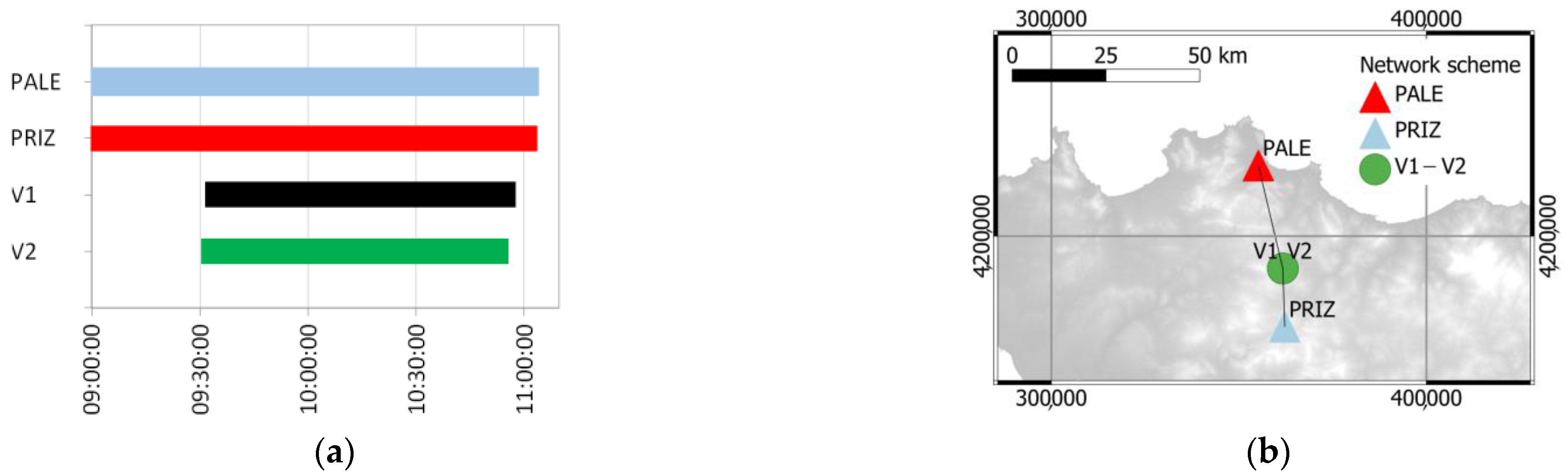
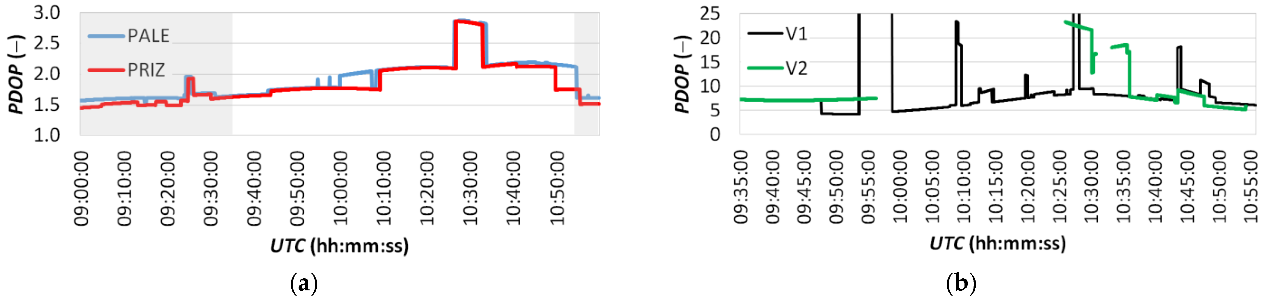
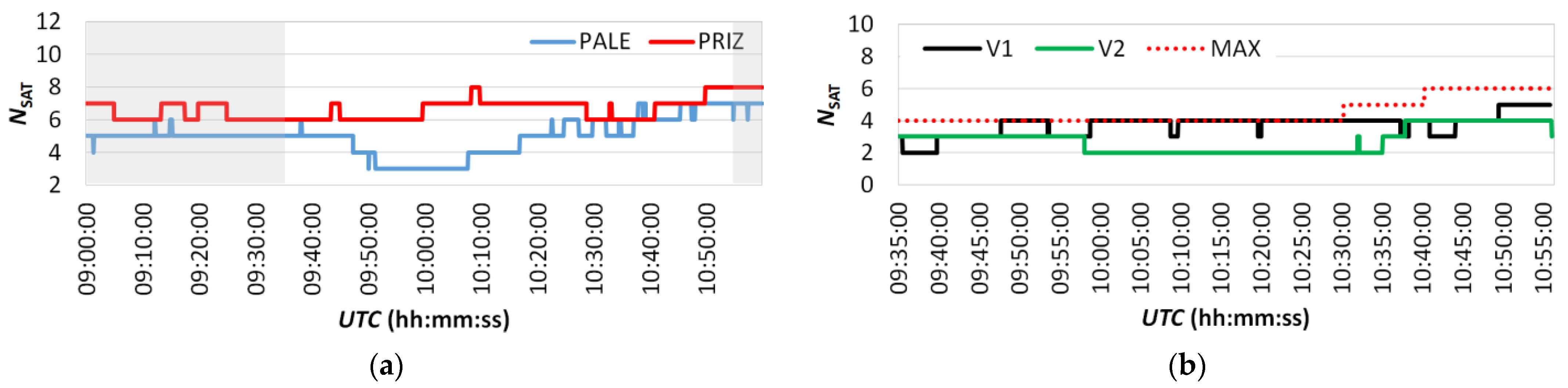
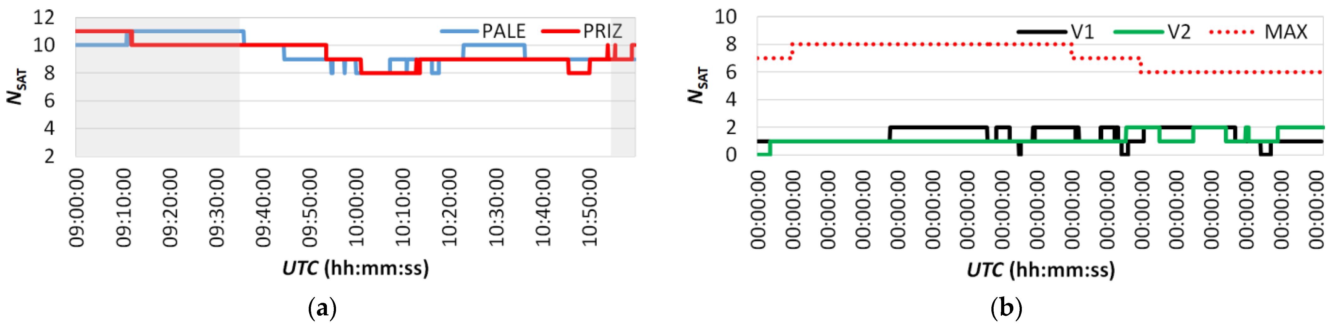
4.1. Tree Positioning via GNSS CORS and Total Station

After checking the overlapping of the data from the two permanent stations of PRIZ and PALE, and the two reference landmarks (Figure 3b), the attention was turned to the assessment of the position PDOP (Figure 4).

The PDOP were excellent [79] (<3) for the two CORS, which were materialized in accordance with EPN requirements at suitable sites with good satellite visibility, while for the two reference landmarks, the PDOP values were moderate–poor, mostly between 5 and 10 (Figure 4b). These PDOP values, which did not meet the standards, were due to the poor signal reception that characterized the acquisitions in the forest, where the presence of very high trees and trees close to each other (heights up to 32 m, with an average distance and standard deviation equal to 4.3 ± 2.5 m and a maximum distance equal to 13.4 m) occluded the satellites’ signal transmissions. Better visibility of the GLONASS constellation (Figure 5) than that of the GPS (Figure 6) was also found during the measurement time window.

The software was not able to fix the solution using GPS first, so according to Dardanelli [87], the solution was initially fixed using the GLONASS constellation alone, which was more accessible, and then the use of the GPS signal allowed the precision of the coordinates of the reference landmarks to be improved (up to centimetric precision) in the short observation period (80′). The maximum number of satellites for the given position, measurement period, and elevation cut-off was over imposed (dashed red line). It was shown that the visible number of satellites at the receiver height (2 m) was much lower than the number of satellites potentially available. The wavelength of the carrier wave indeed only partially passes through the trunk–branches–canopy system (wavelength in the range 18.71–23.79 cm for the GLONASS and in the range 19.03–24.42 cm for the GPS satellites). The number of GLONASS satellites potentially available was lower than that of the GPS. However, the decrease in the number of satellites visible under the crown was stronger for the GPS than for the GLONASS constellation. This resulted in a higher number of GLONASS satellites available than that of the GPS. In addition, the morphology of the mountain area obstructed the visibility of the satellites in some azimuthal sectors until a minimum elevation angle was reached by the satellites [88]. Indeed, in the sectors 50–130, 153–173, and 238–251 degrees (clockwise from north), the satellites became fully visible above an elevation of 22°.

Therefore, the radial-line survey linked the GNSS reference landmarks V1 and V2 (under canopy) allowed the trees in the chosen reference system to be positioned (projected CRS ETRF2000-RDN2008 UTM zone 33N-EPSG: 6708) according to Valbuena et al. [75]. Misclosure root mean squared error (RMSE) was centimetric for both planimetric and altimetric calculations.

Twelve trees, which were visible from a benchmark located in the northern boundary of the study area (V1 of the closed traverse survey), were positioned using a radial line survey through the total station. Distances were measured pointing at a reflector placed on the tree trunk at breast height. These topographic positions allowed it to be established whether those determined via the expeditious survey were reliable for the comparison with the centers of the trees inferable from the ALS survey.

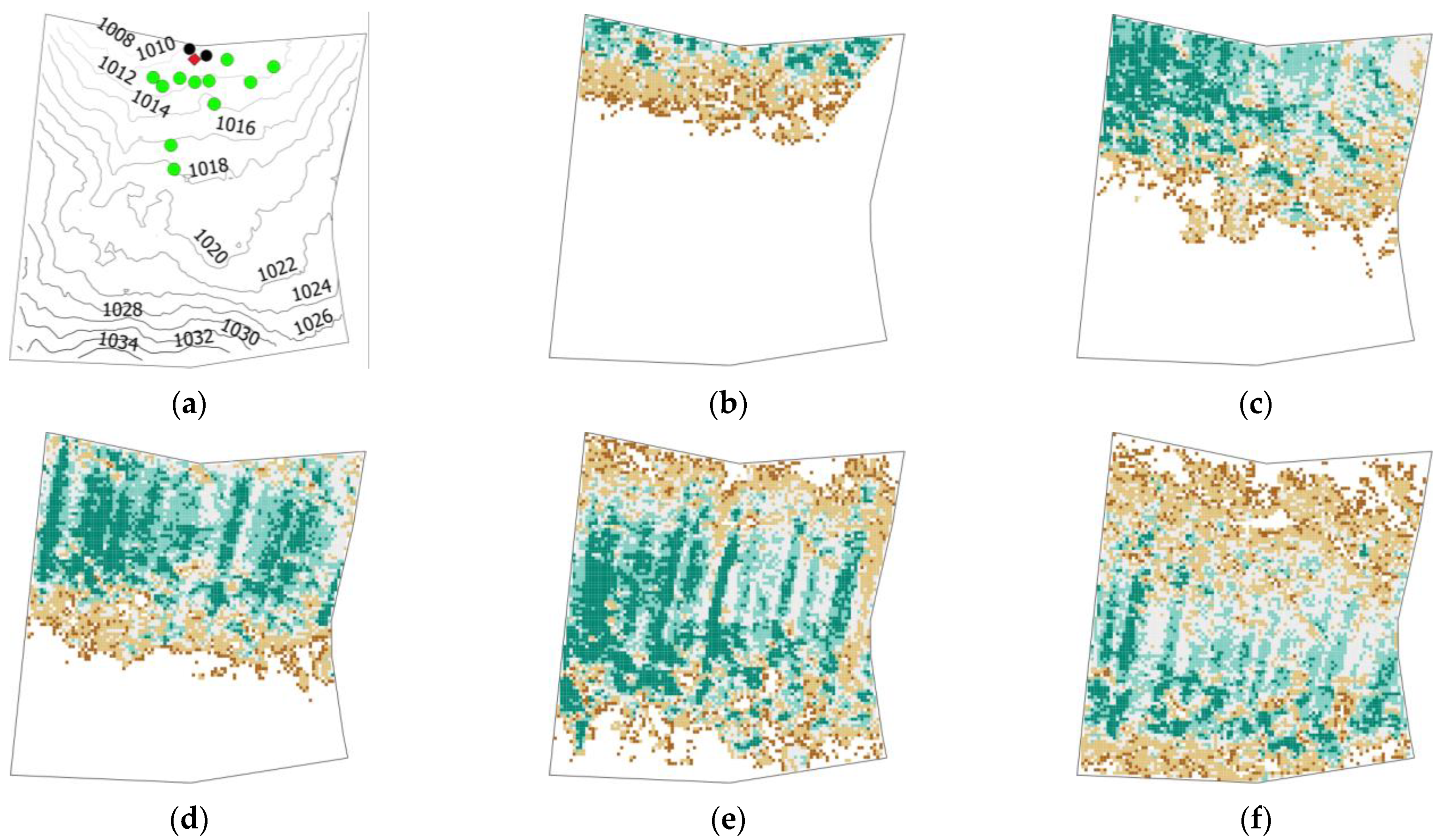
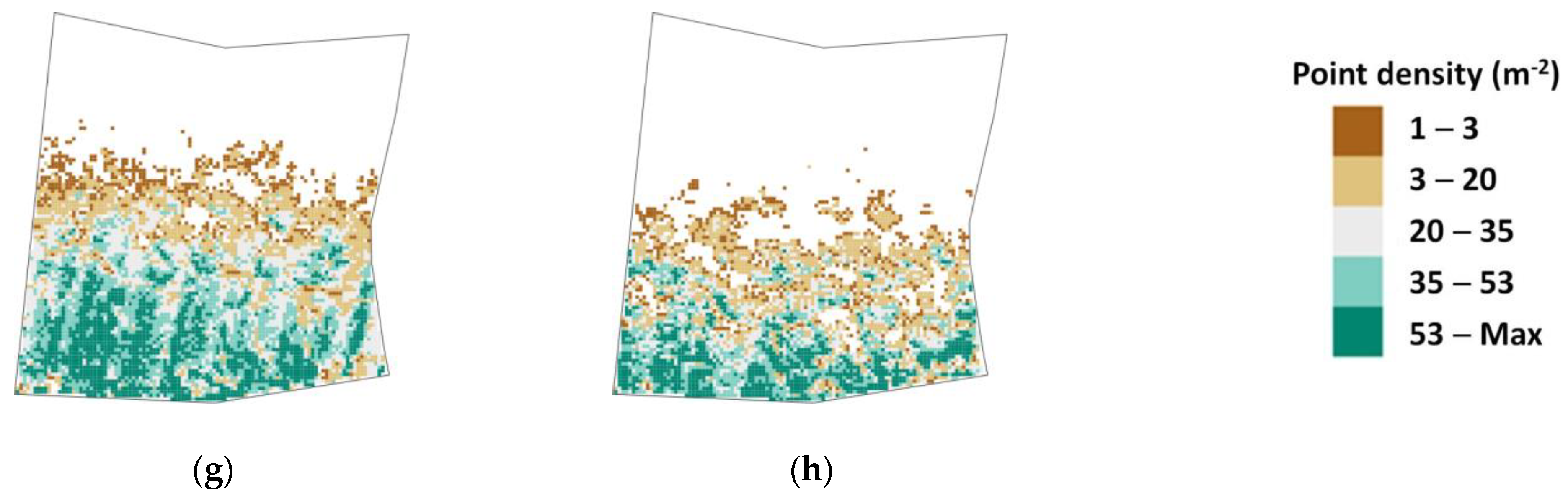
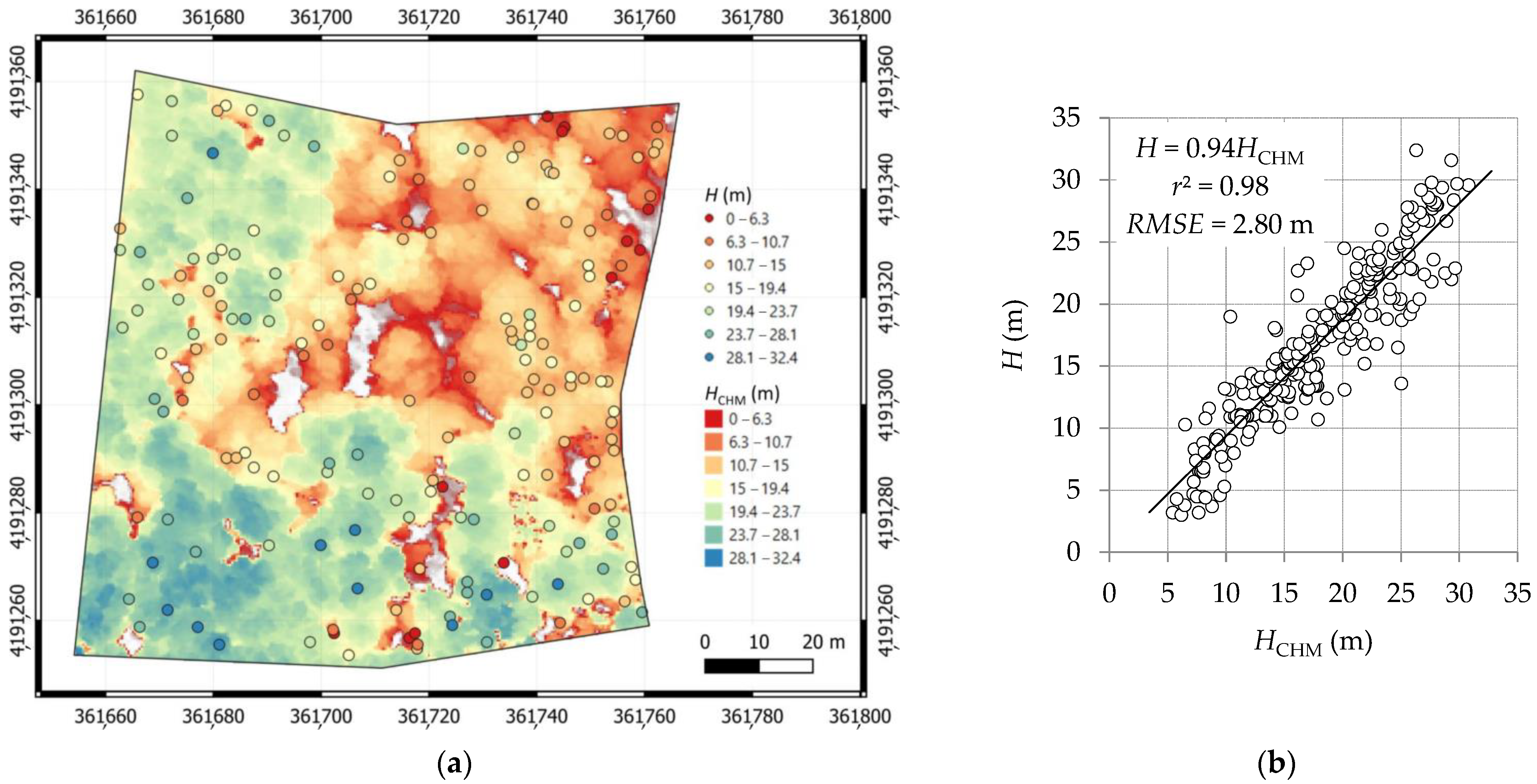
4.2. LIDAR Statistics and Trees’ Topographic Positioning Accuracy

This section reports some statistics describing the merged UAVLS file, and then it analyzes the accuracy in the positioning of the trees with GNSS survey and total station compared to that achieved with the expeditious survey, as well as the accuracy of the heights of the trees derived from laser scanners versus those measured in situ.

The point density (points per square meter) of each strip is reported in Figure 7 (strips S1 to S7 from panel b to h, respectively). The maximum densities were 150, 245, 205, 602, 167, 205, and 244 point m⁻² for the strips S1 to S7, respectively. The color scale was set for the maximum range of variability (1–602, S4). A 5 class equal count diverging color scale was adopted. The color scale was colorblind safe and print friendly.

Once the strips were merged, the number of first returns was 1,159,063, while the number of intermediate returns (5140) was a small percentage (0.4%) of the first ones; instead, the number of last returns (1,155,667) was almost the same number of the first ones (99.7%), and slightly more than the number of single returns (1,010,546, 87.2% of the first ones). The point density of all returns was 122.64 points per square meter, while the spacing of all returns was 0.09 m. Considering the average density of the returns, a spatial resolution ≈5 times higher than the spacing should result in a standard error of the mean not higher than ~20% of the standard deviation of the points generating the pixel value. Thus, the spatial resolution for the DSM model was set to 0.5 m. The same spatial resolution was then chosen for the DTM model.

First returns (Figure 8a) were represented through a 5 class equal count diverging color scale. All the third returns belonged to the first class (panel b). Their density linearly increased with the average altitude (r² = 0.74) as well as with the average slope (r² = 0.54). First returns did not show any trend.

The positions of the trees determined via the topographic survey are reported in Figure 9a (dots). The distances between trees positioned via the expeditious survey and via the topographic survey showed an average value of 4.71 m with a standard error of 0.73 m. This average value was larger than the planimetric absolute accuracy of the YellowScan Mapper integrated system, which was 0.6 m at the flying altitude (50 m). However, considering the uncertainties due to the heterogeneity of (i) the size of the crowns of the dominant trees (characterized by an average radius μ = 3.24 m with standard error σ_μ = 0.12 m); (ii) the eccentricity of the crown (μ = 0.84 m, σ_μ = 0.01 m); and (iii) the tree leaning (μ = 23°, σ_μ = 2.5°) and tree height (μ = 16.5 m, σ_μ = 0.38, maximum height = 32.4 m), it emerged that the accuracy of the expeditious positioning could be considered acceptable.

Dominant, codominant, and intermediate live trees were superimposed as points to the CHM model (Figure 9a). Gaps due to clearings were highlighted in grey. Gaps appeared where dead trees lied on the ground.

Altitudes decrease from southwest to north (from 1034 down to 1008 m). The highest H_CHM values (up to 32.4 m) occurred in the southeast sector, while the lower heights (~2.5 m) resulted in the northwest sector.

The height of the tree measured in situ with this last method was then compared with the H_CHM value of the nearest pixel characterized by an almost null slope and negative curvature (Figure 9b). H_CHM showed a very strong correlation [89] (coefficient of determination r² = 0.98) with the heights of the trees measured in situ, with an average underestimation of 6% (gain equal to 0.94). The root mean square error around the linear trend line was 2.80 m. This value was larger than the integrated system vertical absolute accuracy, which was 0.35 m in this acquisition.

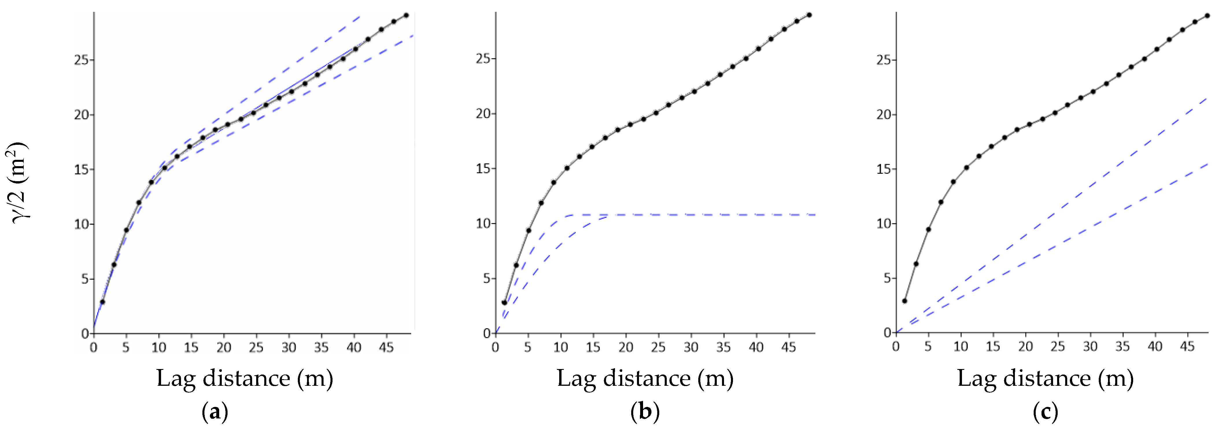
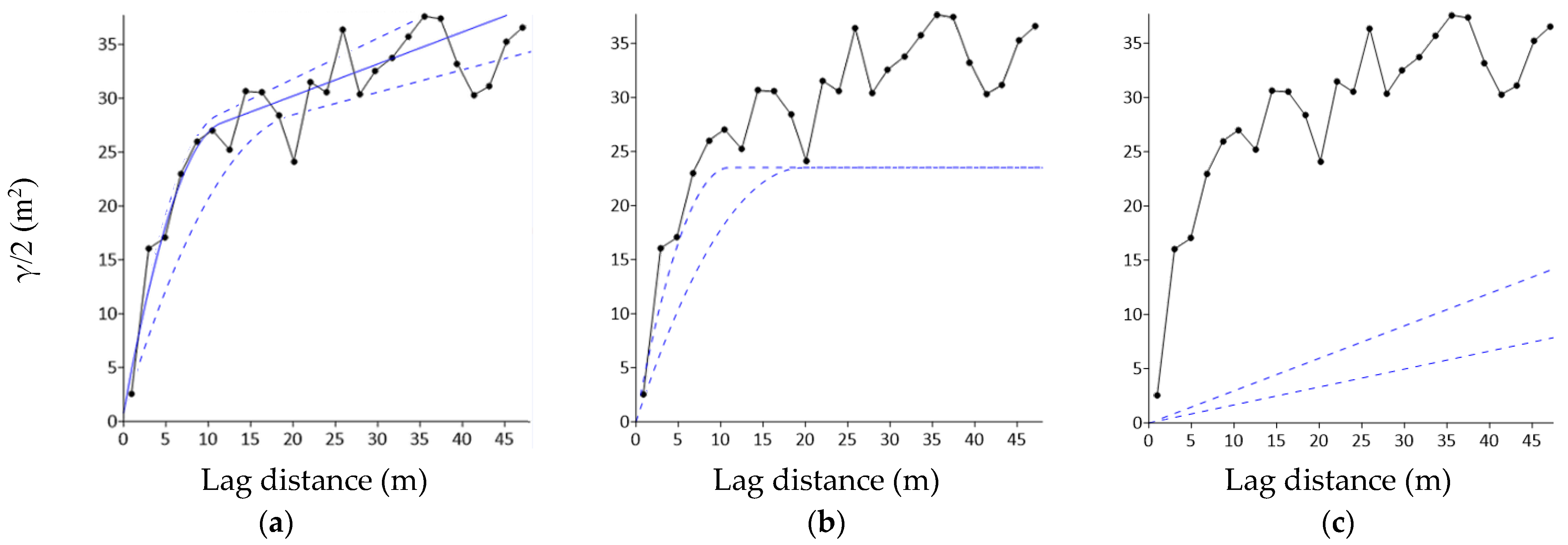
4.3. Semivariogram Analysis

A semivariogram analysis allows the planimetric variability of the trees’ heights of both CHM and H values to be quantified (Figure 10 and Figure 11, respectively). The components’ parameters are reported in

Table 1. The Semivariogram components’ parameters: (a) CHM and (b) H.

Nugget Effect		Quadratic		Nugget Effect		Quadratic
Error	0.61	Scale	10.85	Error	0.78	Scale	23
Variance		Length	20	Variance		Length	20.31
Linear		Anis. ratio	1.66	Linear		Anis. ratio	1.86
Slope	0.32	Anis. angle	90	Slope	0.15	Anis. angle	111
Anis. ratio	1.40			Anis. ratio	2
Anis. angle	145.2			Anis. angle	106.3
(a)				(b)

.

Results showed that the empirical semivariograms (black line with black dots) were in both cases well interpretable by theoretical semivariograms (a panel, blue line) composed of quadratic and linear components (b and c panels, respectively), as well as of a nugget effect.

The empirical semivariogram of H was less uniform than that of the CHM, likely as a consequence of the smaller numerosity of the dataset. The semivariance first grew linearly and suddenly due to a noticeable variability of the height of the trees over short distances, until a lag distance where a knee occurred. Then, for longer lag distances, the semivariance kept increasing linearly although with a smaller slope.

As reported in Table 1, both semivariograms were characterized by anisotropic behavior. For the sake of simplicity, aiming to propose a sampling procedure to apply in the field, we preferred to neglect the effects of anisotropy on sampling plots. Indeed, any sampling criteria accounting for the anisotropy behavior would have been difficult to follow in an operational scenario. The linear component reflected the heights of the trees varying in the south–southwest direction, which roughly constituted a direction of maximum slope. Indeed, the maximum slope between the southern and northern sides of the study area was 0.29 at 5° clockwise from north. The quadratic components (Figure 10b and Figure 11b) showed a sill that is variable with anisotropy (from ~10 to ~20 m). Therefore a size of 20 m was chosen, allowing the value of the sill to be reached independently from the direction and also allowing a higher number of trees to be sampled.

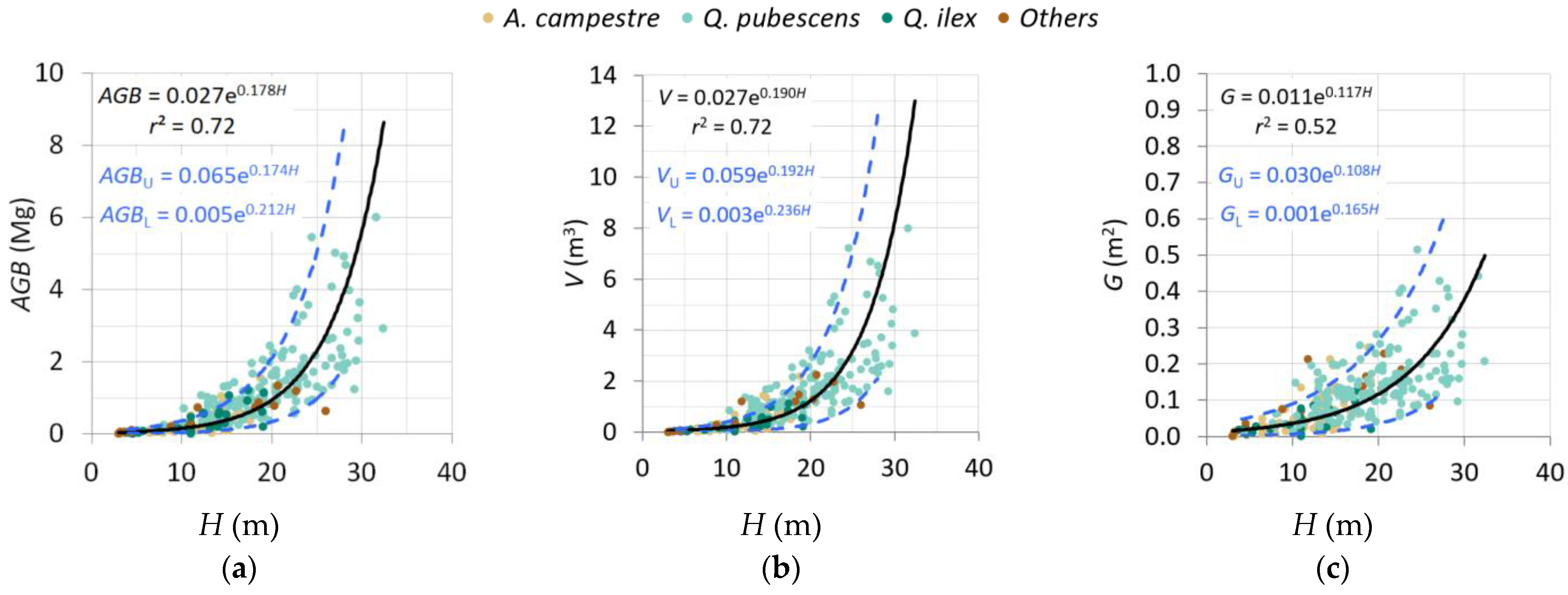
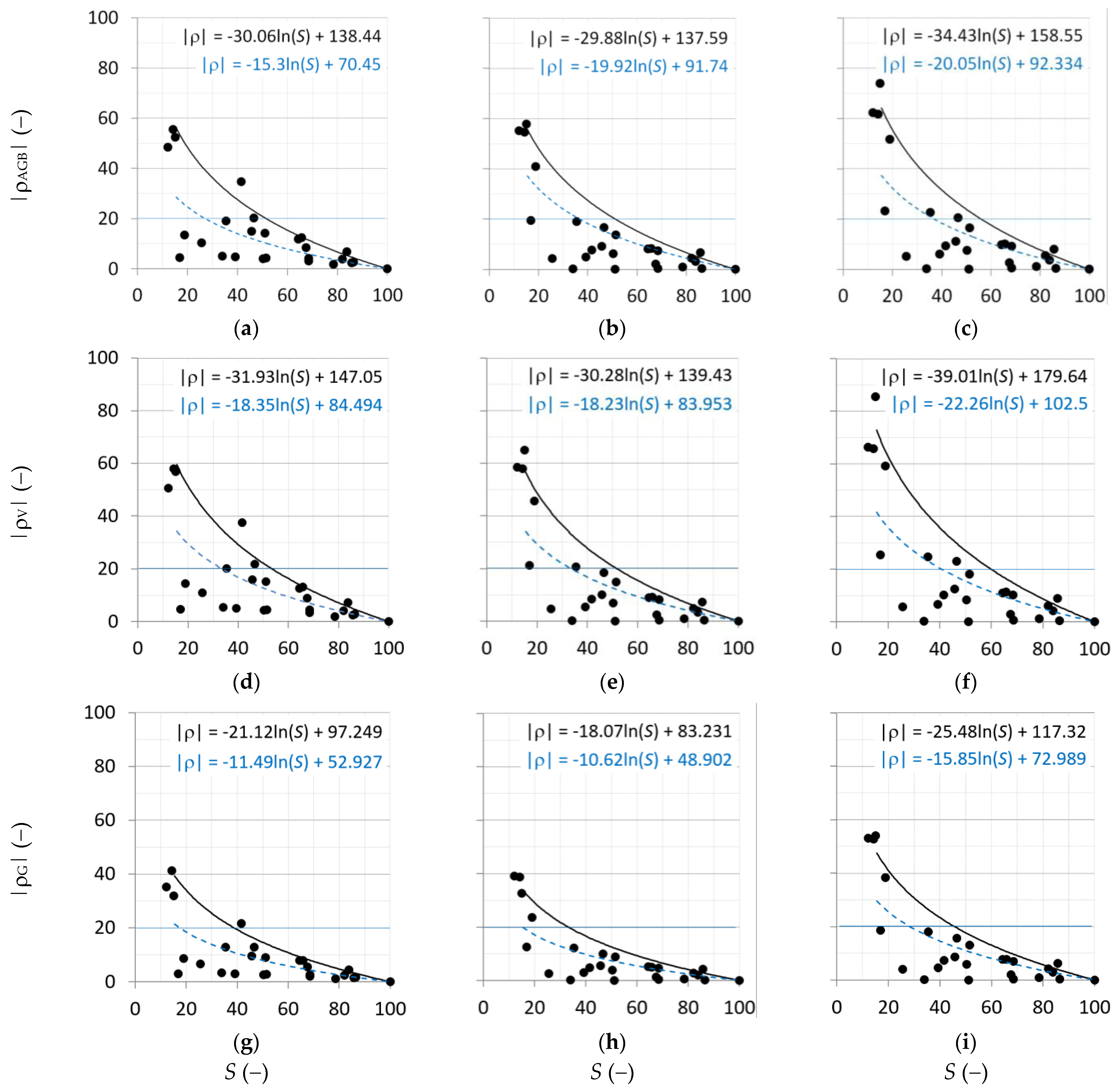
4.4. Sampling Area Optimization

Allometric relationships occur between tree height and the main structural variables employed to describe a forest. Those empirical relationships refer to all the dominant trees as a whole (in Figure 12a–c species are represented with different colors). Interpolation curves of the 5th, 50th, and 95th percentile (lower dashed blue line, black continuous line, and upper dashed blue line, respectively) were over-imposed to help interpret the scatterplots. According to Popescu [21], interpolation curves showed an exponential trend.

The higher the H, the wider the dispersion of AGB(H), V(H), and G(H). Indeed, as the main species of the population (Q. pubescens) extended to the tallest heights, it reached the widest dispersions.

The knee of the semivariogram ruled the gridding of the area into square plots of 20 m side. Then, plots were randomly selected, to investigate the correlation between structural attributes (AGB, V, and G) and tree height (H and H_CHM) for given plots’ numerosity.

The whole plots selection (36 plots, sampling area S = 100) corresponded with sampling the whole trees population. The corresponding values of AGB (Figure 13a–c), V (panels d, e, f), and G (panels g, h, i) for S = 100 were assumed as reference values of the population, thus corresponding to a null apparent relative error (ρ_AGB, ρ_V, ρ_G).

By progressively decreasing the sample size (30, 24, 18, 12, 6, of 36 plots) we characterized gradually smaller surfaces. It should be noted that the presence of boundary plots implies that the surfaces of the plots can be different. As the sample area decreased, the absolute relative errors (|ρ_AGB|, |ρ_V|, |ρ_G| in Figure 10 upper, intermediate, and lower panels, respectively) increased.

Given the dispersion of the structural attributes, it was decided to use the three allometric relationships to quantify the relative errors in determining the structural attributes for different sampling rates. The spatial distributions of AGB, as well as the upper and lower variability AGB_L and AGB_U, were calculated from the average value of the H_CHM of a given number of selected plots and similarly for the other structural attributes V and G.

The interpolation curves of the mean and the 99th percentiles (dashed blue and black curves, respectively) were superimposed to Figure 13 to facilitate its interpretation. The logarithmic curves well described the trend of the data (in Figure 12), and they could be used to quantify the size of the sampling area, assuming an acceptable value of the maximum absolute relative error.

For instance, assuming a tolerable value of the maximum absolute relative error equal to 20% (solid blue horizontal line) in the estimation of the structural attribute, it was sufficient to sample the following:

−

a forest surface between 51% (based on AGB_L, panel c black curve) and 56% (based on AGB_U, panel b black curve), corresponding to an average error varying between 13% (AGB_L, blue dashed curve) and 12% (AGB_U, blue dashed curve);

−

a forest surface between 52% (based on V_L, panel f black curve) and 60% (based on V_U, panel e black curve), corresponding to an average error varying between 12% (V_L, blue dashed curve) and 11% (V_U, blue dashed curve);

−

a forest surface between 33% (based on G_L, panel i, black curve) and 46% (based on G_U, panel h black curve), corresponding to an average error of 12% (for both G_L and G_U, blue dashed curves).

It emerged that the sampling area is a critically important sampling design parameter, as it affects the estimation accuracy of structural attributes of the forest stand. Indeed, the relative error exponentially decreased as the sampling area increased, in agreement with previous studies reporting that the accuracy of the structural attributes estimates improved markedly in terms of coefficient of determination, RMSE, and bias as the sampling area increased six-fold [38] or were duplicated [41]. Some authors suggested a minimum sampling area (500 m²) to provide accurate estimates [16,39]. Several authors [16,38,39,41] concluded that sampling larger areas does not significantly increase the accuracy of the estimates, although it raises the fieldwork cost. In this manuscript, we do not propose a value of sampling area; instead, we propose a methodology to determine the minimum area to be sampled to estimates some forest structural attributes with an acceptable accuracy based on the absolute value of the maximum relative error.

5. Conclusions

The manuscript reported a new methodology for minimizing the sampling area of an old-growth forest, given a tolerable value of the maximum relative error. That area is then characterized by an absolute value of the average relative error. The area is sampled by taking a census of the trees within random plots. The plot size is obtained by analyzing the semivariogram of the heights of the trees. Given a semivariogram component showing a sill, the length (20 m in the present study) is assumed as the minimum dimension characterizing almost the whole variance of forest structural attributes.

A UAV-onboard laser scanner allowed some important forest structural attributes to be estimated with a given accuracy, including aboveground biomass, growing stock volume, and basal area. In addition to UAV laser scanning, the methodology employs GNSS, radial survey, and hypsometric measurements.

Since very high and close trees obstruct the GNSS signal transmission, a strategy to facilitate the positioning was to fix the initial solution by processing only the GLONASS satellites signals (whose visibility was the highest), and then to include the GPS signals to ameliorate the positioning precision (PDOP < ~10).

The heights of the dominant, codominant, and intermediate trees measured in situ were very strongly correlated (r² = 0.98) with those estimated via UAV laser scanning.

Our findings highlighted that assuming a maximum absolute relative error in the estimation of the structural attributes (20% within this work), it is sufficient to sample a part of the investigated forest stand to characterize the whole study area with a low average error (<13%). In particular, we obtained the following maximum values of the sampling surfaces and average absolute errors: a sampling surface of 50% with 13% error for estimating the aboveground biomass; 60% with 12% error for the growing stock volume; and 46% with 12% error for the basal area.

For future studies, we are considering testing the methodology with airborne multi-echo LiDAR products, recently acquired by the Italian “Ministry of the Environment and Land and Sea Protection” (Ministero dell’Ambiente e della Tutela del Territorio e del Mare) as part of an environmental remote sensing plan (Piano Straordinario di Telerilevamento Ambientale). Indeed, a Digital Terrain Model and a Digital Surface Model (first and last returns) are available upon request at 2 m spatial resolution.

Finally, although our methodology has been shown to simplify the characterization of the forest structural attributes, it should be tested on other forest stands having different topographic and structural complexity.

References

- Liu, C.J.; Brantigan, R. Using Differential GPS for Forest Traverse Surveys. Can. J. For. Res. 1995, 25, 1795–1805. [Google Scholar] [CrossRef]
- Sofia, S.; Sferlazza, S.; Mariottini, A.; Niccolini, M.; Coppi, T.; Miozzo, M.; La Mantia, T.; Maetzke, F. A Case Study of The Application of Hand-Held Mobile Laser Scanning in The Planning of An Italian Forest (Alpe Di Catenaia, Tuscany). Int. Arch. Photogramm. Remote Sens. Spatial Inf. Sci. 2021, XLIII-B2-2021, 763–770. [Google Scholar] [CrossRef]
- Krause, S.; Sanders, T.G.M.; Mund, J.-P.; Greve, K. UAV-Based Photogrammetric Tree Height Measurement for Intensive Forest Monitoring. Remote Sens. 2019, 11, 758. [Google Scholar] [CrossRef] [Green Version]
- Lechner, A.M.; Foody, G.M.; Boyd, D.S. Applications in Remote Sensing to Forest Ecology and Management. One Earth 2020, 2, 405–412. [Google Scholar] [CrossRef]
- Sferlazza, S.; Maltese, A.; Ciraolo, G.; Dardanelli, G.; Maetzke, F.G.; La Mela Veca, D.S. Forest Accessibility, Madonie Mountains (Northern Sicily, Italy): Implementing a GIS Decision Support System. J. Maps 2021, 17, 476–485. [Google Scholar] [CrossRef]
- Wallace, L.; Musk, R.; Lucieer, A. An Assessment of the Repeatability of Automatic Forest Inventory Metrics Derived From UAV-Borne Laser Scanning Data. IEEE Trans. Geosci. Remote Sens. 2014, 52, 7160–7169. [Google Scholar] [CrossRef]
- Gatziolis, D.; Fried, J.S.; Monleon, V.S. Challenges to Estimating Tree Height via LiDAR in Closed-Canopy Forests: A Parable from Western Oregon. For. Sci. 2010, 56, 139–155. [Google Scholar]
- Mielcarek, M.; Stereńczak, K.; Khosravipour, A. Testing and Evaluating Different LiDAR-Derived Canopy Height Model Generation Methods for Tree Height Estimation. Int. J. Appl. Earth Obs. Geoinf. 2018, 71, 132–143. [Google Scholar] [CrossRef]
- Popescu, S.C.; Wynne, R.H.; Nelson, R.F. Estimating Plot-Level Tree Heights with Lidar: Local Filtering with a Canopy-Height Based Variable Window Size. Comput. Electron. Agric. 2002, 37, 71–95. [Google Scholar] [CrossRef]
- Wang, Y.; Lehtomäki, M.; Liang, X.; Pyörälä, J.; Kukko, A.; Jaakkola, A.; Liu, J.; Feng, Z.; Chen, R.; Hyyppä, J. Is Field-Measured Tree Height as Reliable as Believed—A Comparison Study of Tree Height Estimates from Field Measurement, Airborne Laser Scanning and Terrestrial Laser Scanning in a Boreal Forest. ISPRS J. Photogramm. Remote Sens. 2019, 147, 132–145. [Google Scholar] [CrossRef]
- Popescu, S.C.; Wynne, R.H.; Nelson, R.F. Measuring Individual Tree Crown Diameter with Lidar and Assessing Its Influence on Estimating Forest Volume and Biomass. Can. J. Remote Sens. 2003, 29, 564–577. [Google Scholar] [CrossRef]
- Coops, N.C.; Hilker, T.; Wulder, M.A.; St-Onge, B.; Newnham, G.; Siggins, A.; Trofymow, J.A. Estimating Canopy Structure of Douglas-Fir Forest Stands from Discrete-Return LiDAR. Trees-Struct. Funct. 2007, 21, 295–310. [Google Scholar] [CrossRef] [Green Version]
- Roberts, S.; Dean, T.J.; Evans, D.L.; McCombs, J.; Harrington, R.L.; Glass, P.A. Estimating Individual Tree Leaf Area in Loblolly Pine Plantations Using LiDAR-Derived Measurements of Height and Crown Dimensions. For. Ecol. Manag. 2009, 213, 54–70. [Google Scholar] [CrossRef]
- García-Cimarras, A.; Manzanera, J.A.; Valbuena, R. Analysis of Mediterranean Vegetation Fuel Type Changes Using Multitemporal Lidar. Forests 2021, 12, 335. [Google Scholar] [CrossRef]
- Solano, F.; Praticò, S.; Piovesan, G.; Modica, G. Unmanned Aerial Vehicle (UAV) Derived Canopy Gaps in the Old-Growth Beech Forest of Mount Pollinello (Italy): Preliminary Results. In Computational Science and Its Applications—ICCSA 2021; Gervasi, O., Murgante, B., Misra, S., Garau, C., Blečić, I., Taniar, D., Apduhan, B.O., Rocha, A.M.A.C., Tarantino, E., Torre, C.M., Eds.; Lecture Notes in Computer Science; Springer International Publishing: Cham, Switzerland, 2021; Volume 12955, pp. 126–138. ISBN 978-3-030-87006-5. [Google Scholar]
- Anderson, R.S.; Bolstad, P.V. Estimating Aboveground Biomass and Average Annual Wood Biomass Increment with Airborne Leaf-on and Leaf-off Lidar in Great Lakes Forest Types. North. J. Appl. For. 2013, 30, 16–22. [Google Scholar] [CrossRef]
- Bottalico, F.; Chirici, G.; Giannini, R.; Mele, S.; Mura, M.; Puxeddu, M.; McRoberts, R.E.; Valbuena, R.; Travaglini, D. Modeling Mediterranean Forest Structure Using Airborne Laser Scanning Data. Int. J. Appl. Earth Obs. Geoinf. 2017, 57, 145–153. [Google Scholar] [CrossRef]
- Chirici, G.; McRoberts, R.E.; Fattorini, L.; Mura, M.; Marchetti, M. Comparing Echo-Based and Canopy Height Model-Based Metrics for Enhancing Estimation of Forest Aboveground Biomass in a Model-Assisted Framework. Remote Sens. Environ. 2016, 174, 1–9. [Google Scholar] [CrossRef]
- Corona, P.; Cartisano, R.; Salvati, R.; Chirici, G.; Floris, A.; di Martino, P.; Marchetti, M.; Scrinzi, G.; Clementel, F.; Travaglini, D.; et al. Airborne Laser Scanning to Support Forest Resource Management under Alpine, Temperate and Mediterranean Environments in Italy. Eur. J. Remote Sens. 2012, 45, 27–37. [Google Scholar] [CrossRef] [Green Version]
- Næsset, E. Predicting Forest Stand Characteristics with Airborne Scanning Laser Using a Practical Two-Stage Procedure and Field Data. Remote Sens. Environ. 2002, 80, 88–99. [Google Scholar] [CrossRef]
- Popescu, S.C. Estimating Biomass of Individual Pine Trees Using Airborne Lidar. Biomass Bioenergy 2007, 31, 646–655. [Google Scholar] [CrossRef]
- Ruiz, L.A.; Hermosilla, T.; Mauro, F.; Godino, M. Analysis of the Influence of Plot Size and LiDAR Density on Forest Structure Attribute Estimates. Forests 2014, 5, 936–951. [Google Scholar] [CrossRef] [Green Version]
- Holmgren, J.; Nilsson, M.; Olsson, H. Estimation of Tree Height and Stem Volume on Plots Using Airborne Laser Scanning. For. Sci. 2003, 49, 419–428. [Google Scholar] [CrossRef]
- McRoberts, R.E.; Tomppo, E.O.; Næsset, E. Advances and Emerging Issues in National Forest Inventories. Scand. J. For. Res. 2010, 25, 368–381. [Google Scholar] [CrossRef]
- Hyyppä, J.; Yu, X.; Hyyppä, H.; Vastaranta, M.; Holopainen, M.; Kukko, A.; Kaartinen, H.; Jaakkola, A.; Vaaja, M.; Koskinen, J.; et al. Advances in Forest Inventory Using Airborne Laser Scanning. Remote Sens. 2012, 4, 1190–1207. [Google Scholar] [CrossRef] [Green Version]
- Forestry Applications of Airborne Laser Scanning: Concepts and Case Studies; Maltamo, M.; Næsset, E.; Vauhkonen, J. (Eds.) Managing Forest Ecosystems; Springer: Dordrecht, The Netherlands, 2014; Volume 27, ISBN 978-94-017-8662-1. [Google Scholar]
- Latifi, H.; Fassnacht, F.E.; Müller, J.; Tharani, A.; Dech, S.; Heurich, M. Forest Inventories by LiDAR Data: A Comparison of Single Tree Segmentation and Metric-Based Methods for Inventories of a Heterogeneous Temperate Forest. Int. J. Appl. Earth Obs. Geoinf. 2015, 42, 162–174. [Google Scholar] [CrossRef]
- White, J.C.; Coops, N.C.; Wulder, M.A.; Vastaranta, M.; Hilker, T.; Tompalski, P. Remote Sensing Technologies for Enhancing Forest Inventories: A Review. Can. J. Remote Sens. 2016, 42, 619–641. [Google Scholar] [CrossRef] [Green Version]
- Means, J.E.; Acker, S.A.; Fitt, B.J.; Renslow, M.; Emerson, L.; Hendrix, C.J. Predicting Forest Stand Characteristics with Airborne Scanning Lidar. Photogramm. Eng. Remote Sens. 2000, 66, 1367–1371. [Google Scholar]
- Seidl, R.; Spies, T.A.; Rammer, W.; Steel, E.A.; Pabst, R.J.; Olsen, K. Multi-Scale Drivers of Spatial Variation in Old-Growth Forest Carbon Density Disentangled with Lidar and an Individual-Based Landscape Model. Ecosystems 2012, 15, 1321–1335. [Google Scholar] [CrossRef] [Green Version]
- Sverdrup-Thygeson, A.; Ørka, H.O.; Gobakken, T.; Næsset, E. Can Airborne Laser Scanning Assist in Mapping and Monitoring Natural Forests? For. Ecol. Manag. 2016, 369, 116–125. [Google Scholar] [CrossRef]
- White, J.C.; Tompalski, P.; Coops, N.C.; Wulder, M.A. Comparison of Airborne Laser Scanning and Digital Stereo Imagery for Characterizing Forest Canopy Gaps in Coastal Temperate Rainforests. Remote Sens. Environ. 2018, 208, 1–14. [Google Scholar] [CrossRef]
- Bauhus, J.; Puettmann, K.; Messier, C. Silviculture for Old-Growth Attributes. For. Ecol. Manag. 2009, 258, 525–537. [Google Scholar] [CrossRef] [Green Version]
- Burrascano, S.; Keeton, W.S.; Sabatini, F.M.; Blasi, C. Commonality and Variability in the Structural Attributes of Moist Temperate Old-Growth Forests: A Global Review. For. Ecol. Manag. 2013, 291, 458–479. [Google Scholar] [CrossRef]
- Lindenmayer, D.B.; Franklin, J.F. Conserving Forest Biodiversity: A Comprehensive Multiscaled Approach; Island Press: Washington, DC, USA, 2002; ISBN 978-1-55963-935-4. [Google Scholar]
- Shorohova, E.; Kneeshaw, D.; Kuuluvainen, T.; Gauthier, S. Variability and Dynamics of Old-Growth Forests in the Circumboreal Zone: Implications for Conservation, Restoration and Management. Silva. Fenn. 2011, 45, 785–806. [Google Scholar] [CrossRef] [Green Version]
- Jiang, Y.; Kim, J.B.; Trugman, A.T.; Kim, Y.; Still, C.J. Linking Tree Physiological Constraints with Predictions of Carbon and Water Fluxes at an Old-Growth Coniferous Forest. Ecosphere 2019, 10, e02692:20. [Google Scholar] [CrossRef] [Green Version]
- McGarvey, J.C.; Thompson, J.R.; Epstein, H.E.; Shugart, H.H., Jr. Carbon Storage in Old-Growth Forests of the Mid-Atlantic: Toward Better Understanding the Eastern Forest Carbon Sink. Ecology 2015, 96, 311–317. [Google Scholar] [CrossRef]
- Corona, P.; Blasi, C.; Chirici, G.; Facioni, L.; Fattorini, L.; Ferrari, B. Monitoring and Assessing Old-Growth Forest Stands by Plot Sampling. Plant. Biosyst. 2010, 144, 171–179. [Google Scholar] [CrossRef] [Green Version]
- Motta, R.; Garbarino, M.; Berretti, R.; Bjelanovic, I.; Borgogno Mondino, E.; Čurović, M.; Keren, S.; Meloni, F.; Nosenzo, A. Structure, Spatio-Temporal Dynamics and Disturbance Regime of the Mixed Beech–Silver Fir–Norway Spruce Old-Growth Forest of Biogradska Gora (Montenegro). Plant. Biosyst.-An. Int. J. Deal. All Asp. Plant. Biol. 2015, 149, 966–975. [Google Scholar] [CrossRef]
- Paillet, Y.; Pernot, C.; Boulanger, V.; Debaive, N.; Fuhr, M.; Gilg, O.; Gosselin, F. Quantifying the Recovery of Old-Growth Attributes in Forest Reserves: A First Reference for France. For. Ecol. Manag. 2015, 346, 51–64. [Google Scholar] [CrossRef]
- Barabesi, L.; Fattorini, L. The Use of Replicated Plot, Line and Point Sampling for Estimating Species Abundance and Ecological Diversity. Environ. Ecol. Stat. 1998, 5, 353–370. [Google Scholar] [CrossRef]
- Alessandrini, A.; Biondi, F.; Di Filippo, A.; Ziaco, E.; Piovesan, G. Tree Size Distribution at Increasing Spatial Scales Converges to the Rotated Sigmoid Curve in Two Old-Growth Beech Stands of the Italian Apennines. For. Ecol. Manag. 2011, 262, 1950–1962. [Google Scholar] [CrossRef]
- Frazer, G.W.; Magnussen, S.; Wulder, M.A.; Niemann, K.O. Simulated Impact of Sample Plot Size and Co-Registration Error on the Accuracy and Uncertainty of LiDAR-Derived Estimates of Forest Stand Biomass. Remote Sens. Environ. 2011, 115, 636–649. [Google Scholar] [CrossRef]
- Lombardi, F.; Marchetti, M.; Corona, P.; Merlini, P.; Chirici, G.; Tognetti, R.; Burrascano, S.; Alivernini, A.; Puletti, N. Quantifying the Effect of Sampling Plot Size on the Estimation of Structural Indicators in Old-Growth Forest Stands. For. Ecol. Manag. 2015, 346, 89–97. [Google Scholar] [CrossRef] [Green Version]
- McRoberts, R.E.; Winter, S.; Chirici, G.; LaPoint, E. Assessing Forest Naturalness. For. Sci. 2012, 58, 294–309. [Google Scholar] [CrossRef]
- Gobakken, T.; Næsset, E. Assessing Effects of Positioning Errors and Sample Plot Size on Biophysical Stand Properties Derived from Airborne Laser Scanner Data. Can. J. For. Res. 2009, 39, 1036–1052. [Google Scholar] [CrossRef]
- Zhao, K.; Popescu, S.; Nelson, R. Lidar Remote Sensing of Forest Biomass: A Scale-Invariant Estimation Approach Using Airborne Lasers. Remote Sens. Environ. 2009, 113, 182–196. [Google Scholar] [CrossRef]
- Calamini, G.; Maltoni, A.; Travaglini, D.; Iovino, F.; Nicolaci, A.; Menguzzato, G.; Corona, P.; Ferrari, B.; Santo, D.D.; Chirici, G.; et al. Caratteri Strutturali Di Potenziali Foreste Vetuste Appenniniche: Risultati Preliminari. L’Italia For. E Mont. 2011, 66, 365–381. [Google Scholar] [CrossRef] [Green Version]
- Motta, R.; Garbarino, M.; Berretti, R.; Meloni, F.; Nosenzo, A.; Vacchiano, G. Development of Old-Growth Characteristics in Uneven-Aged Forests of the Italian Alps. Eur. J. For. Res. 2015, 134, 19–31. [Google Scholar] [CrossRef] [Green Version]
- Nagel, T.A.; Svoboda, M. Gap Disturbance Regime in an Old-Growth Fagus–Abies Forest in the Dinaric Mountains, Bosnia-Herzegovina. Can. J. For. Res. 2008, 38, 2728–2737. [Google Scholar] [CrossRef] [Green Version]
- Badalamenti, E.; La Mantia, T.; La Mantia, G.; Cairone, A.; La Mela Veca, D.S. Living and Dead Aboveground Biomass in Mediterranean Forests: Evidence of Old-Growth Traits in a Quercus Pubescens Willd. s.l. Stand. Forests 2017, 8, 187. [Google Scholar] [CrossRef] [Green Version]
- Rivas-Martínez, S.; Penas, A.; Díaz, T. Biogeographic Map of Europe; Cartographic service: Léon, Spain, 2004. [Google Scholar]
- Food and Agriculture Organization World Reference Base for Soil Resources 2014: International Soil Classification System for Naming Soils and Creating Legends for Soil Maps; FAO: Rome, Italy, 2014; ISBN 978-92-5-108369-7.
- Kattenborn, T.; Sperlich, M.; Bataua, K.; Koch, B. Automatic Single Palm Tree Detection in Plantations Using UAV-Based Photogrammetric Point Clouds. Int. Arch. Photogramm. Remote Sens. Spat. Inf. Sci. 2014, XL–3, 139–144. [Google Scholar] [CrossRef] [Green Version]
- Balsi, M.; Esposito, S.; Fallavollita, P.; Nardinocchi, C. Single-Tree Detection in High-Density LiDAR Data from UAV-Based Survey. Eur. J. Remote Sens. 2018, 51, 679–692. [Google Scholar] [CrossRef] [Green Version]
- Andritsanos, V.D.; Arabatzi, O.; Gianniou, M.; Pagounis, V.; Tziavos, I.N.; Vergos, G.S.; Zacharis, E. Comparison of Various GPS Processing Solutions toward an Efficient Validation of the Hellenic Vertical Network: The ELEVATION Project. J. Surv. Eng. 2016, 142, 04015007:13. [Google Scholar] [CrossRef]
- Mageed, K.M.A. Comparison of GPS Commercial Software Packages to Processing Static Baselines up to 30 Km. ARPN J. Eng. Appl. Sci. 2015, 10, 10640–10650. [Google Scholar]
- Dardanelli, G.; Paliaga, S.; Allegra, M.; Carella, M.; Giammarresi, V. Geomatic Applications Tourban Park in Palermo. Geogr. Tech. 2015, 10, 28–43. [Google Scholar]
- Goad, C.C. A Modified Hopfield Tropospheric Refraction Correction Model. Paper presented at the Fall Annual Meeting American Geophysical Union, San Francisco, CA, USA, 12–17 December 1974. [Google Scholar]
- Hopfield, H.S. Two-Quartic Tropospheric Refractivity Profile for Correcting Satellite Data. J. Geophys. Res. 1969, 74, 4487–4499. [Google Scholar] [CrossRef]
- Niell, A.E. Global Mapping Functions for the Atmosphere Delay at Radio Wavelengths. J. Geophys. Res. B Solid Earth 1996, 101, 3227–3246. [Google Scholar] [CrossRef]
- Coulson, D.M.; Roth, K.C. Gemini North r’ Band Imaging of the Keck II Laser. In Proceedings of the SPIE Proceedings; Ellerbroek, B.L., Hart, M., Hubin, N., Wizinowich, P.L., Eds.; International Society for Optics and Photonics: San Diego, CA, USA, 2010; Volume 7736, p. 9. [Google Scholar]
- Trimble GNSS Planning. Available online: https://www.gnssplanning.com/#/settings (accessed on 21 February 2022).
- Sferlazza, S.; Maetzke, F.; Iovino, M.; Baiamonte, G.; Palmeri, V.; La Mela Veca, D.S. Effects of Traditional Forest Management on Carbon Storage in a Mediterranean Holm Oak (Quercus Ilex L.) Coppice. Iforest-Biogeosci. For. 2018, 11, 344–351. [Google Scholar] [CrossRef] [Green Version]
- Ward, J.; Anagnostakis, S.; Ferrandino, F. Stand Dynamics in Connecticut Hardwood Forests: The Old Series Plots (1927–1997); Connecticut Agricultural Experiment Station: New Haven, CT, USA, 1999. [Google Scholar]
- Tabacchi, G.; Di Cosmo, L.; Gasparini, P. Aboveground Tree Volume and Phytomass Prediction Equations for Forest Species in Italy. Eur. J. Forest Res. 2011, 130, 911–934. [Google Scholar] [CrossRef]
- Meyer, T.; Bean, J.; Ferguson, C.; Naismith, J. The Effect of Broadleaf Canopies on Survey-Grade Horizontal GPS/GLONASS Measurements; Department of Natural Resources and the Environment Articles; UCONN: Storrs, CT, USA, 2002. [Google Scholar]
- Lachapelle, G. Pedestrian Navigation with High Sensitivity GPS Receivers and MEMS. Pers. Ubiquitous Comput. 2007, 11, 481–488. [Google Scholar] [CrossRef]
- Fauzi, M.F.; Idris, N.H.; Yahya, M.H.; Din, A.H.M.; Idris, N.H.; Lau, A.M.S.; Ishak, M.H.L. Tropical Forest Tree Positioning Accuracy: A Comparison of Low Cost GNSS-Enabled Devices. Int. J. Geoinform. 2016, 12, 59–66. [Google Scholar]
- Tomaštík, J.; Varga, M. Practical Applicability of Processing Static, Short-Observation-Time Raw GNSS Measurements Provided by a Smartphone under Tree Vegetation. Measurement 2021, 178, 109397. [Google Scholar] [CrossRef]
- Fan, Y.; Feng, Z.; Mannan, A.; Khan, T.U.; Shen, C.; Saeed, S. Estimating Tree Position, Diameter at Breast Height, and Tree Height in Real-Time Using a Mobile Phone with RGB-D SLAM. Remote Sens. 2018, 10, 1845. [Google Scholar] [CrossRef] [Green Version]
- Kaartinen, H.; Hyyppä, J.; Vastaranta, M.; Kukko, A.; Jaakkola, A.; Yu, X.; Pyörälä, J.; Liang, X.; Liu, J.; Wang, Y.; et al. Accuracy of Kinematic Positioning Using Global Satellite Navigation Systems under Forest Canopies. Forests 2015, 6, 3218–3236. [Google Scholar] [CrossRef]
- Næsset, E.; Gjevestad, J.G. Performance of GPS Precise Point Positioning Under Conifer Forest Canopies. Photogramm Eng Remote Sens. 2008, 74, 661–668. [Google Scholar] [CrossRef]
- Valbuena, R.; Mauro, F.; Rodriguez-Solano, R.; Manzanera, J.A. Accuracy and Precision of GPS Receivers under Forest Canopies in a Mountainous Environment. Span. J. Agric. Res. 2010, 8, 1047. [Google Scholar] [CrossRef]
- Dardanelli, G.; Lo Brutto, M.; Pipitone, C. GNSS CORS Network of the University of Palermo: Design and First Analysis of Data. Geog. Techn. 2020, 15, 43–69. [Google Scholar] [CrossRef]
- Kenyeres, A.; Bellet, J.G.; Bruyninx, C.; Caporali, A.; de Doncker, F.; Droscak, B.; Duret, A.; Franke, P.; Georgiev, I.; Bingley, R.; et al. Regional Integration of Long-Term National Dense GNSS Network Solutions. GPS Solut 2019, 23, 122. [Google Scholar] [CrossRef] [Green Version]
- Dardanelli, G.; Maltese, A.; Pipitone, C.; Pisciotta, A.; Lo Brutto, M. Nrtk, Ppp or Static, That Is the Question. Testing Different Positioning Solutions for Gnss Survey. Remote Sens. 2021, 13, 1406. [Google Scholar] [CrossRef]
- Mikulski, J. Modern Transport. Telematics: 11th International Conference on Transport. Systems Telematics, TST 2011, Katowice-Ustron, Poland, October 19–22, 2011, Selected Papers; Springer Science & Business Media: Berlin/Heidelberg, Germany, 2011; ISBN 978-3-642-24659-3. [Google Scholar]
- Kissam, P. Surveying for Civil. Engineers; McGraw-Hill: New York, NY, USA, 1981; ISBN 978-0-07-034882-0. [Google Scholar]
- Kraus, K.; Pfeifer, N. Determination of Terrain Models in Wooded Areas with Airborne Laser Scanner Data. ISPRS J. Photogramm. Remote Sens. 1998, 53, 193–203. [Google Scholar] [CrossRef]
- Biondi, F.; Myers, D.E.; Avery, C.C. Geostatistically Modeling Stem Size and Increment in an Old-Growth Forest. Can. J. For. Res. 1994, 24, 1354–1368. [Google Scholar] [CrossRef]
- Kuuluvainen, T.; Penttinen, A.; Leinonen, K.; Nygren, M. Statistical Opportunities for Comparing Stand Structural Heterogeneity in Managed and Primeval Forests: An Example from Boreal Spruce Forest in Southern Finland. Silva. Fennica 1996, 30, 315–328. [Google Scholar] [CrossRef] [Green Version]
- Kuuluvainen, T.; Järvinen, E.; Hokkanen, T.J.; Rouvinen, S.; Heikkinen, K. Structural Heterogeneity and Spatial Autocorrelation in a Natural Mature Pinus Sylvestris Dominated Forest. Ecography 1998, 21, 159–174. [Google Scholar] [CrossRef]
- Rozas, V.; Zas, R.; Solla, A. Spatial Structure of Deciduous Forest Stands with Contrasting Human Influence in Northwest Spain. Eur. J. Forest Res. 2009, 128, 273–285. [Google Scholar] [CrossRef] [Green Version]
- Song, C. Estimating Tree Crown Size with Spatial Information of High Resolution Optical Remotely Sensed Imagery. Int. J. Remote Sens. 2007, 28, 3305–3322. [Google Scholar] [CrossRef]
- Dardanelli, G. Valutazione dell’apporto della costellazione GLONASS nel posizionamento NRTK con ricevitori GNSS geodetici. GEOmedia 2011, 15, 40–46. [Google Scholar]
- Lu, Y.-H.; Han, J.-Y. Gnss Satellite Visibility Analysis Based on 3d Spatial Information in Urban Areas. Int. Arch. Photogramm. Remote Sens. Spatial Inf. Sci. 2020, XLIII-B4-2020, 123–128. [Google Scholar] [CrossRef]
- Evans, J.D. Straightforward Statistics for the Behavioral Sciences; Brooks/Cole Pub. Co.: Pacific Grove, CA, USA, 1996; ISBN 978-0-534-23100-2. [Google Scholar]