Article

Modelling, Validation and Quantification of Climate and Other Sensitivities of Building Energy Model on 3D City Models †

1
European Institute for Energy Research, 76131 Karlsruhe, Germany
2
School of Computer Science and Electrical Engineering, CentraleSupélec, 91190 Gif-sur-Yvette, France
*
Author to whom correspondence should be addressed.
This paper is an extended version of our paper published in Murshed SM, Picard S and Koch A. (2017) CityBEM: An Open Source Implementation and Validation of Monthly Heating and Cooling Energy Needs for 3D Buildings in Cities. ISPRS Annals of the Photogrammetry, Remote Sensing and Spatial Information Sciences IV-4/W5: 83-90.
ISPRS Int. J. Geo-Inf. 2018, 7(11), 447; https://0-doi-org.brum.beds.ac.uk/10.3390/ijgi7110447
Submission received: 1 September 2018 / Revised: 30 October 2018 / Accepted: 7 November 2018 / Published: 15 November 2018

Abstract

:
New planning tools are required to depict the complete building stock in a city and investigate detailed measures on reaching local and global targets to improve energy efficiency and reduce greenhouse gas emissions. To pursue this objective, ISO (the International Organization for Standardization) 13790:2008 monthly heating and cooling energy calculation method is implemented using geometric information from 3D city models (e.g., CityGML format) in an open source software architecture. A model is developed and applied in several urban districts with different number of 3D buildings in various cities. The model is validated with the simulation software TRNSYS. We also perform a sensitivity analysis to quantify the impact of climate change and other physical and behavioral factors on modelling results. The proposed approach can help to perform city or district-wide analysis of the building energy needs and prepare different renovation plans to support decision-making, which finally will enhance the livability of a city and the quality of life of the citizens.

1. Introduction

Cities play an important role in reaching local and global targets to improve energy efficiency and reduce greenhouse gas emissions. In order to determine the potential of energy efficiency in the building sector, new planning instruments are required that allow depicting the complete building stock on the one hand, and investigate detailed measures on the other hand. This can be achieved by assessing the building heating and cooling energy needs with detailed data on buildings stocks. In this regard, 3D city models can provide more realistic geometry and forms of the buildings, as well as various other input parameters such as building typology and energy characteristics associated with the 3D data. The studies on Building Energy Modelling (BEM) and their implementation at various spatial and temporal scales have been performed for a number of years. Statistical and engineering models are used for a multitude of applications [1], e.g., in low carbon energy strategies [2], increasing the energy efficiency for building refurbishment plans [3], etc. Statistical models are highly dependent on historical data of energy use, whereas engineering models are based on the physical properties of buildings and heat transfer calculations. The advantages and disadvantages for such modelling approaches at the scale of neighborhoods are reviewed by References [4,5,6,7].

1.1. ISO Method Applied Without 3D City Models

ISO 13790:2008 calculation method provides a deterministic model to calculate heating and cooling energy needs of buildings at three different temporal resolutions: hourly, monthly and seasonal [8]. It is one of a series of calculation methods for the design and evaluation of energy performance of buildings. Many studies have applied the monthly and hourly approaches with different assumptions and contexts. Several national authorities have also adopted a performance-based method using a monthly energy balance, for example Romania [9] or South Korea [10]. Vollaro et al. [11] calculated the monthly cooling and heating energy performance of an old building in central Italy using the ISO 13790 based software named MC11300. The results were validated with dynamic simulation software (TRNSYS). Kim et al. [12] compared the simplified ISO 13790 method and dynamic (EnergyPlus software) simulation approach with regard to uncertainty. The different simulations were tested on a general five-story office building in the South Korea. They highlighted the importance of calibration for unknown parameters (numerical parameters and time constants) in a local application of the ISO 13790 monthly method. Kristensen et al. [13] investigated the monthly and the hourly ISO 13790 method considering a building zone test case located in Denmark. Kokogiannakis et al. [14] carried out a comparative analysis of the hourly and monthly ISO 13790 methods with simulation programs (e.g., ESP-r and EnergyPlus). Several parameters of a typical office building were varied by considering different climate, internal heat gains, glazing areas, ventilation schedules, etc. Corrado et al. [15] proposed a useful implementation of the ISO 13790 monthly calculation method, in particular to supply a formulation of the dynamic parameters and adapt them to the local climate. The simulation was performed on some real buildings in Italy, assuming different climatic conditions. The method was then validated with EnergyPlus. Within the framework of a EU project ENTRANZE [16], cooling and heating energy demand of four different building types across 10 European cities (Seville, Madrid, Rome, Milan, Bucharest, Vienna, Paris, Prague, Berlin and Helsinki) were performed by EnergyPlus simulation software. The results were compared with the ISO 13790 hourly (implemented in spreadsheet) and ISO 13790 monthly (INVERT/EE-Lab program) methods. They concluded that due to different calculation approaches and different degrees of complexities of the building and usage description in the three simulation tools, the energy needs varied significantly. Furthermore, the hourly and monthly methods were applied in an office building in Finland [17] and the results were validated with the IDA-ICE building energy software, considering it as a reference. Vartieres et al. [18] applied three different modelling approaches (e.g., ISO 13790 monthly, CODYBA and TRNSYS) to calculate the cooling energy demand of an office building in Bucharest. Then, a comparative assessment on the modelling input parameters and results were performed.
Some studies have performed sensitivity analysis of the ISO 13790:2008 method to identify and rank the uncertain input parameters and to explore the behavior of related models [19,20,21,22,23]. Recently, Kristensen and Petersen [13] gave a comprehensive overview of different local and global sensitivity approaches and compared three different but most commonly used sensitivity analysis methods, namely Local, Morris and Sobol. The methods were discussed for a building zone, representing a residential building stock, using the hourly and monthly models of ISO 13790. They found that the local method was just as capable of identifying the most important parameters as the more sophisticated Morris and Sobol’s method, but it was not capable of identifying the same ranking of parameters in terms of importance to the model output. Earlier, Kim et al. [12] carried out a sensitivity analysis using Morris method to identify the most dominant input parameters and to rank them with respect to simulation output. For the monthly ISO 13790 method, they found out that the number of people per area, the ventilation coefficient, the set point temperature, the internal heat flow, and the conductivity of insulation are the most influencing parameters.

1.2. ISO Method Applied on 3D City Models

Today, standardized semantic 3D city models in the CityGML format in different levels of detail (LOD1, LOD2, etc.) are available in many cities in the world [24]. This enables researchers and practitioners to simulate the physical behaviour of buildings with modelling approaches like the ISO 13790:2008 method [8] in order to carry out city-wide calculations of building energy needs. Many recent studies have pointed out the potential for such applications [3,25], but only few studies have considered the 3D building characteristics as inputs into the ISO calculation method to analyse both heating and cooling energy needs for a large number of buildings in a district or a city. Chalal et al. [5] performed a critical literature review of mainly 2D and 3D Geographic Information System (GIS) based approaches for energy prediction models. Eicker et al. [26] calculated the monthly heat demand in three districts in Germany using the 3D city models and applying the German standard DIN 18599. Later, Nouvel et al. [27] implemented the monthly ISO 13790 method with the 3D buildings data to calculate heating energy needs in the two residential districts in Karlsruhe (LOD1) and Ludwigsburg (LOD2). Recently, Nouvel et al. [2] attempted to combine a statistical and engineering modelling approach to ascertain the building heating needs in order to support urban energy policies on buildings. Agugiaro [28] calculated the residential energy demand for both space heating and hot water following the simplified calculation procedure, as described by the Technical Specification UNI/TS 11300:2008-National annex to CEN (European Committee for Standardization) standards (parts 1 and 2) in Italy. In this regard, the LOD2 data of the part of city of Trento was chosen as the study area. However, the validation and sensitivity analyses of the models were not performed.

1.3. Research Gaps

Based on the literature review on the implementation of ISO 13790:2008 method, we observe that simulation was mostly performed on individual buildings. Some tools were developed for specific purposes and few open source implementations were realized. Some recent studies have adopted the 3D city models to assess energy needs based on country specific norms in some particular sectors (e.g., residential buildings). None of them were performed for both the heating and cooling energy need. Some studies based on 3D city models performed validation of ISO method using consumption data; others did not perform robust validation of their implementation. All the studies performed the sensitivity of one building at a time; so far, none of them performed the analysis using 3D city models together with future climate scenarios. The former especially allows assessing the impact of the quality of urban data models with regard to the calculated energy needs.

1.4. Objectives of the Paper

Considering the research gaps, the main objectives of this paper are to
  • implement the ISO method using the 3D city models to calculate the building heating and cooling energy needs on monthly basis (CityBEM model),
  • develop an easy to use software architecture to carry out a quick and robust analysis,
  • consider the buildings (geometry and attributes) of the 3D city models at a district or city scale and use publicly available datasets,
  • perform a robust validation of the model,
  • perform 3D visualization and analysis of results, and
  • quantify the sensitivity of climate change and model parameters on monthly heating and cooling energy needs.

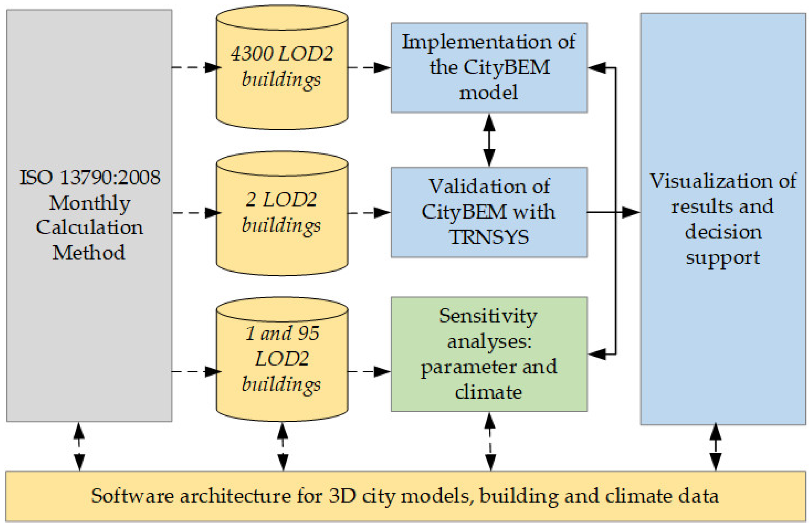
2. Methodological Approach
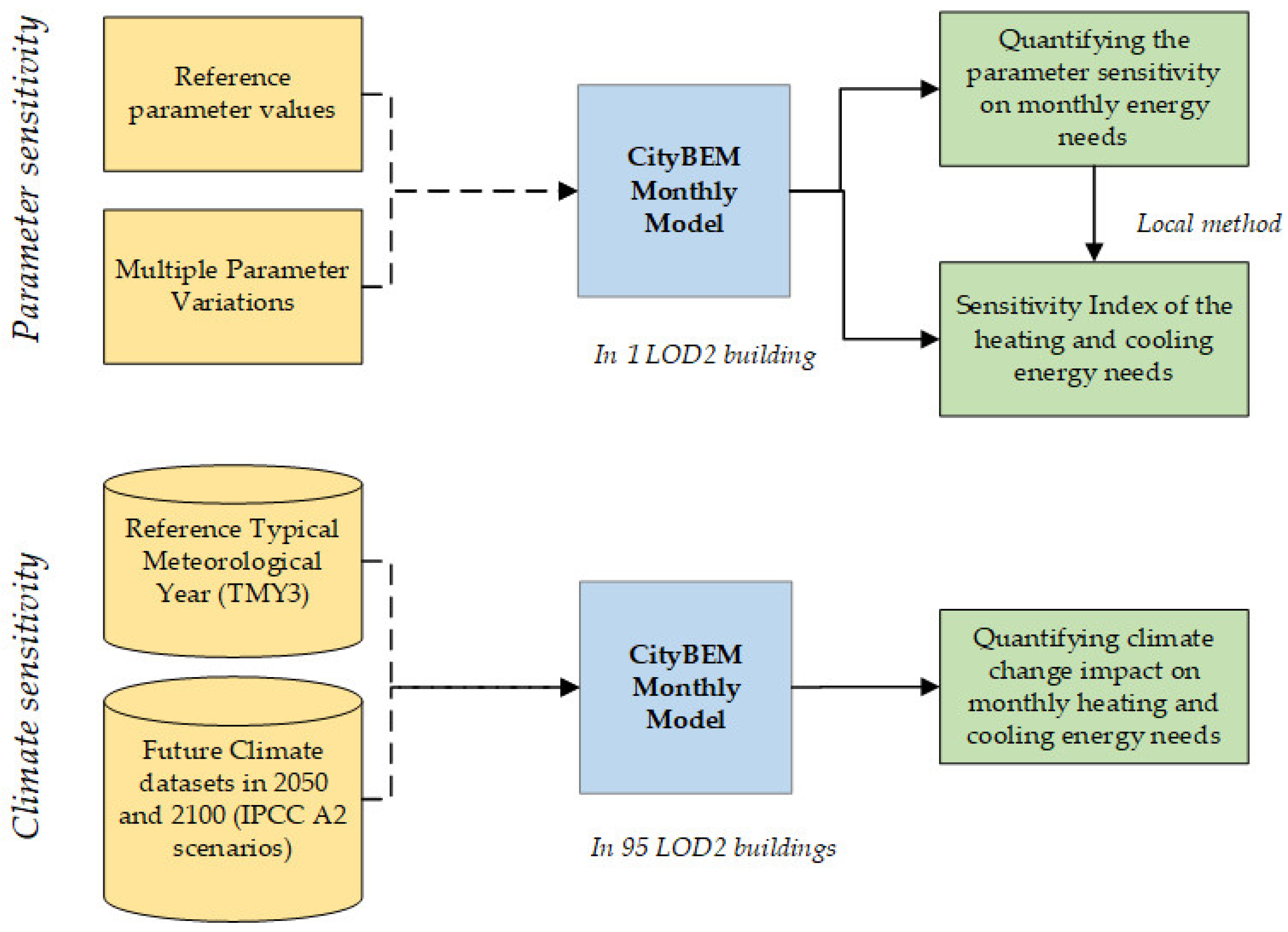
2.1. Overview

The overall research methodology of this study is explained in Figure 1. The different components such as the description of the ISO method and its implementation, software architecture, 3D city models and other data, validation and sensitivity analyses are described in the following sections.

2.2. ISO 13790:2008 Monthly Calculation Method

The ISO 13790:2008 monthly method is developed at a macroscopic level of thermal gains and losses and is based on the simplified representation of building physics. It takes into account dynamic effects by empirically determined utilization factors for heat losses or gains. The model calculates heating or cooling monthly energy needs, based on the balance between the transmission and ventilation heat losses as well as the internal and solar gains, in interaction with the building mass, external factors and occupants’ behavior [8]. The ISO method is structured into four main blocks:
  • Definition of building boundaries for conditioned and unconditioned spaces,
  • Identification of the zones (single vs. multi zones),
  • Definition of the internal conditions for calculation of external climate, and other environmental data inputs (heat transfer losses, heat gain, etc.),
  • Calculation of energy needs for heating and cooling, for each time step and building.
The monthly method is used worldwide by different national energy standard organizations and the results are proven accurate and robust in a long-term urban energy scenario development for a district having hundreds of buildings [2]. Advantages are highlighted in several studies, e.g., References [8,12], etc. (see Section 1). The monthly ISO method also produces good results compared to other software such as EnergyPlus [13]. It is also proven that this simplified quasi-steady state monthly method is able to predict year-round energy needs, provided that the dynamic parameters are correctly determined [15].

2.3. Required Input Data and Data Handling

Three categories of input data are required for the monthly model: Building geometry, building typology and climate conditions (Table 1). The 3D city models having the original roof structure in the LOD2 helps to accurately calculate the building geometry related characteristics, such as the volume and floor area. The building typologies and their physical characteristics, such as heat transfer coefficients (U value), ventilation rate, technical system etc., are based on empirical studies carried out by the Institute for housing and environment (Institut Wohnen und Umwelt GmbH, IWU). The climate conditions such as wind speed, temperature and solar radiation have a significant impact on the building energy needs. They are collected from the Meteonorm 7.1 software on a Typical Meteorological Year (TMY3) ([29]). The average monthly solar radiation for every building surface is calculated from the PLANTING model [30,31]. It performs numeric calculation on hourly incoming solar radiation and energy production from photovoltaic panels on the horizontal and vertical surfaces of the buildings, by considering the shading from the neighboring buildings or terrains.

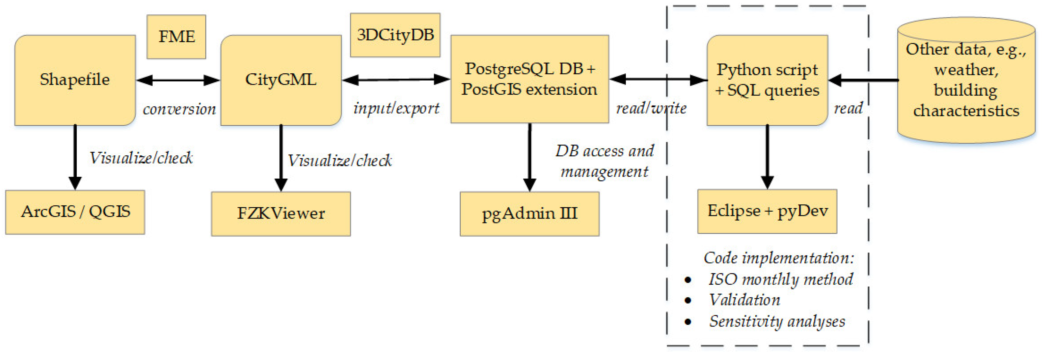
2.4. Software Architecture

Several software and tools are required to prepare the different data formats, as well as to implement and calculate the monthly energy needs of the 3D building. They are mainly open source and freely available (Figure 2).
LOD2 CityGML data on building was imported into the PostgreSQL/3DCityDB database with information about the geometry and the building coordinates. The 3DCityDB (http://www.3dcitydb.org/3dcitydb) is a free open source package consisting of a database schema and a set of software tools to import, manage, analyze, visualize, and export virtual 3D city models according to the CityGML standard. This software includes a tool for importing CityGML data into a PostgreSQL database. Then, using a Python script, the surface and volume of each building was calculated within the Eclipse environment. Eclipse is deployed to create a base workspace and an extensible plug-in system for customizing the environment. For this study, the PyDev plug-in (http://www.pydev.org) was used to work with Python scripts. Python supports connection to the PostgreSQL database (https://www.postgresql.org). Building typology datasets were collected in excel or CSV format. The climate data on monthly average temperature and wind speed were extracted from the Meteonorm 7.1 software as CSV format. They were processed using Python scripts and stored as different tables in the PostgreSQL database (Figure 2). Other tools such as FZKViewer (https://www.iai.kit.edu/1302.php), QGIS, FME, pgAdmin III were also utilized to create the software architecture.

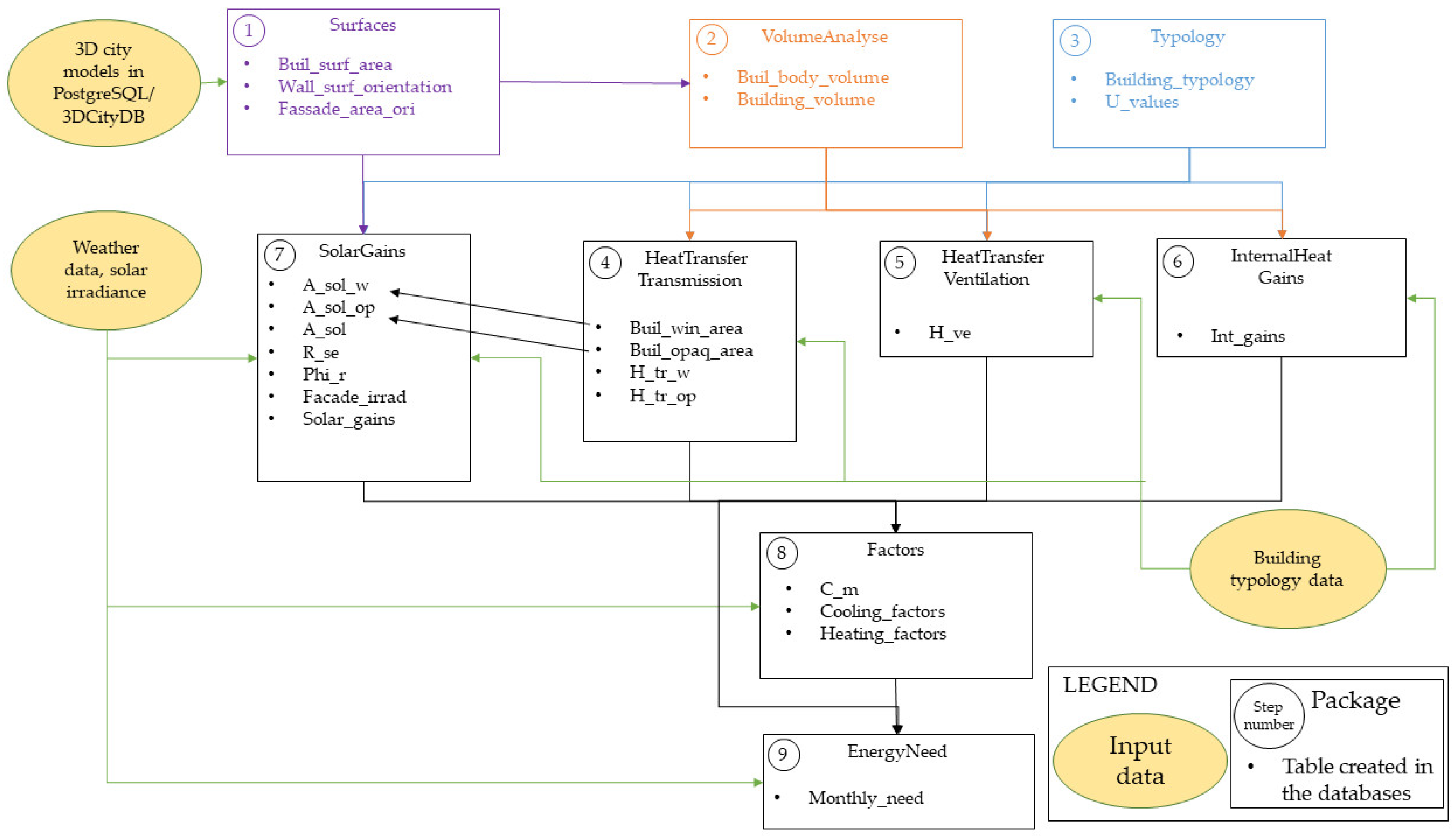
3. Implementation of the ISO Method

For each building in the 3D city model, the energy needs for heating and cooling for each month was calculated after the suggestions provided by the ISO method. However, it is assumed that (a) each building is modelled as single zone; (b) the set-point temperatures, internal gains and air change rates are averaged according to the respective conditioned used area and (c) reduction factor is taken into account for calculating intermittence heating and cooling need.
The ISO method is implemented in seven main steps [8]:
  • Calculation of heat transfer coefficients by transmission ( H t r ) and ventilation ( H v e )
  • Calculation of the total heat transfer ( Q h t ) from transmission and ventilation, assuming the time step t of one month
    Q h t = Q t r + Q v e = ( H t r + H v e ) ( θ i n t , s e t θ e ) t
  • Calculation of heat flow coefficients from solar radiation ( Q ˙ s o l ) and internal sources ( Q ˙ i n t )
  • Calculation of total heat gains ( Q g n ) from the internal and solar heat gains, assuming the time step t of one month
    Q g n = Q i n t + Q s o l = ( Q ˙ i n t + Q ˙ s o l ) t
  • Calculation of the dynamic parameters: η l s utilization factor for heat losses (cooling mode), η g n utilization factor for heat gains (heating mode)
  • Reduction factor for intermittent cooling ( a C , r e d ) and heating ( a H , r e d )
  • Calculation of cooling and heating need:
    • For the cooling mode:
      Q C , n d = Q g n η l s Q h t
      Q C , n d , i n t e r m = a C , r e d Q C , n d
    • For the heating mode:
      Q H , n d = Q h t η g n Q g n
      Q H , n d , i n t e r m = a H , r e d Q H , n d
      where,
      • Htr and Hve  Heat transfer coefficients by transmission and ventilation in W/K
      • Qint and Qsol   Heat flow coefficients from internal sources and solar radiations in W
      • Qht        Total heat transfer (transmission and ventilation) in MJ
      • Qgn       Total heat gains (solar and internal gains) in MJ
      • t          Time step in month
      • ηls         Utilization factor for heat losses (no dimension)
      • ηgn        Utilization factor for heat gains (no dimension)
      • aC, red      Reduction factor for cooling (no dimension)
      • aH, red      Reduction factor for heating (no dimension)
      • QC, nd      Energy need for the continuous cooling mode in MJ
      • QH, nd        Energy need for the continuous heating mode in MJ
      • QC, nd, interm    Energy need for the intermittent cooling mode in MJ
      • QH, nd, interm   Energy need for the intermittent heating mode in MJ
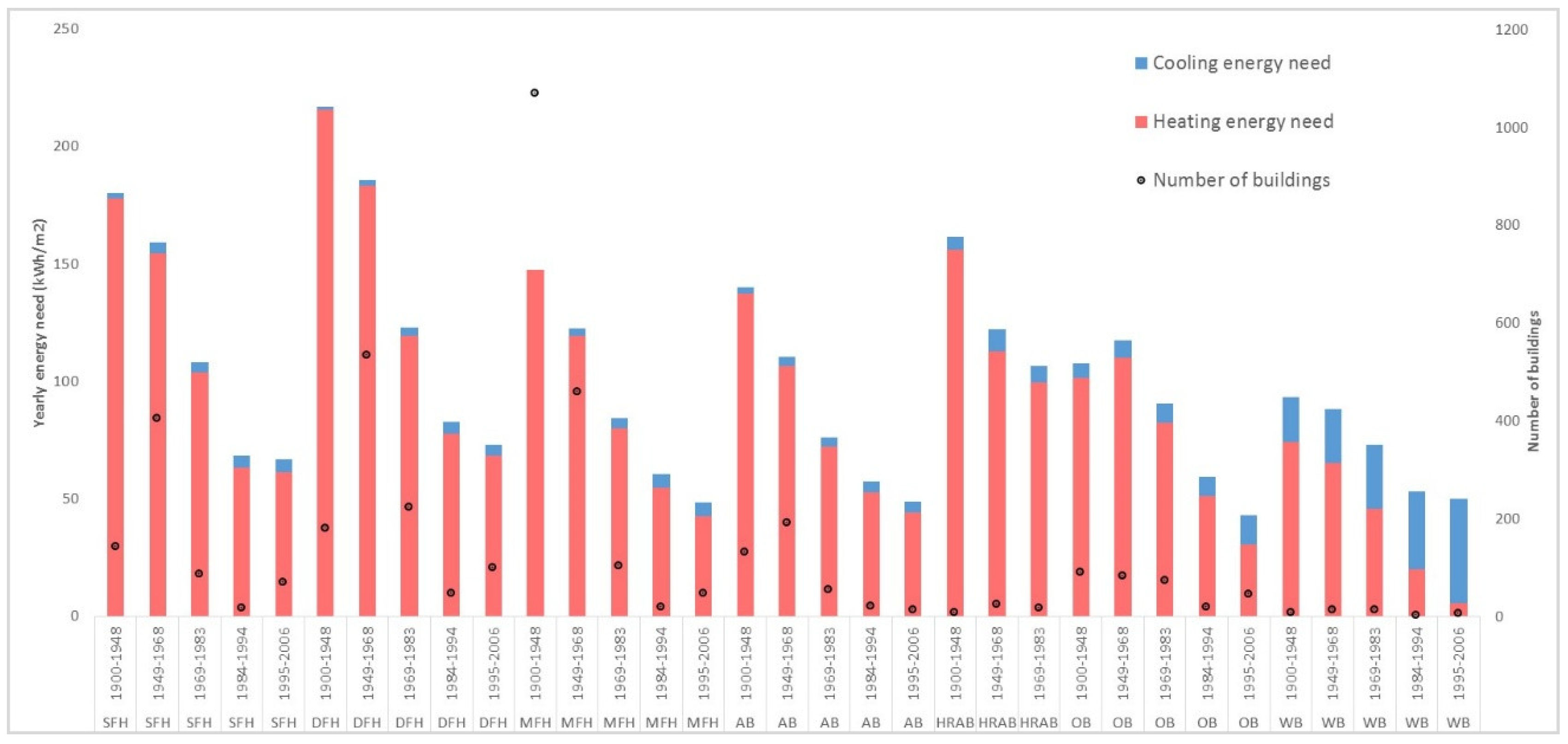
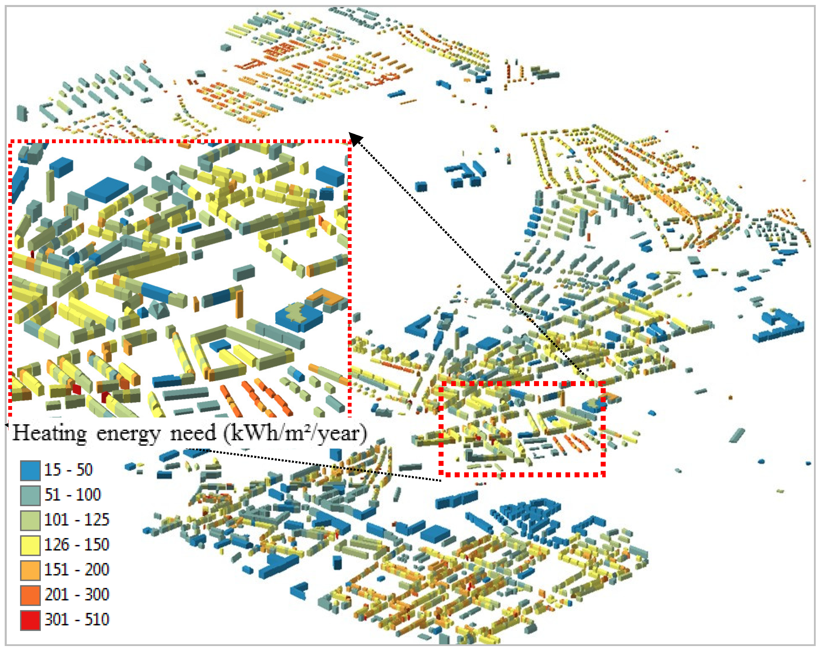
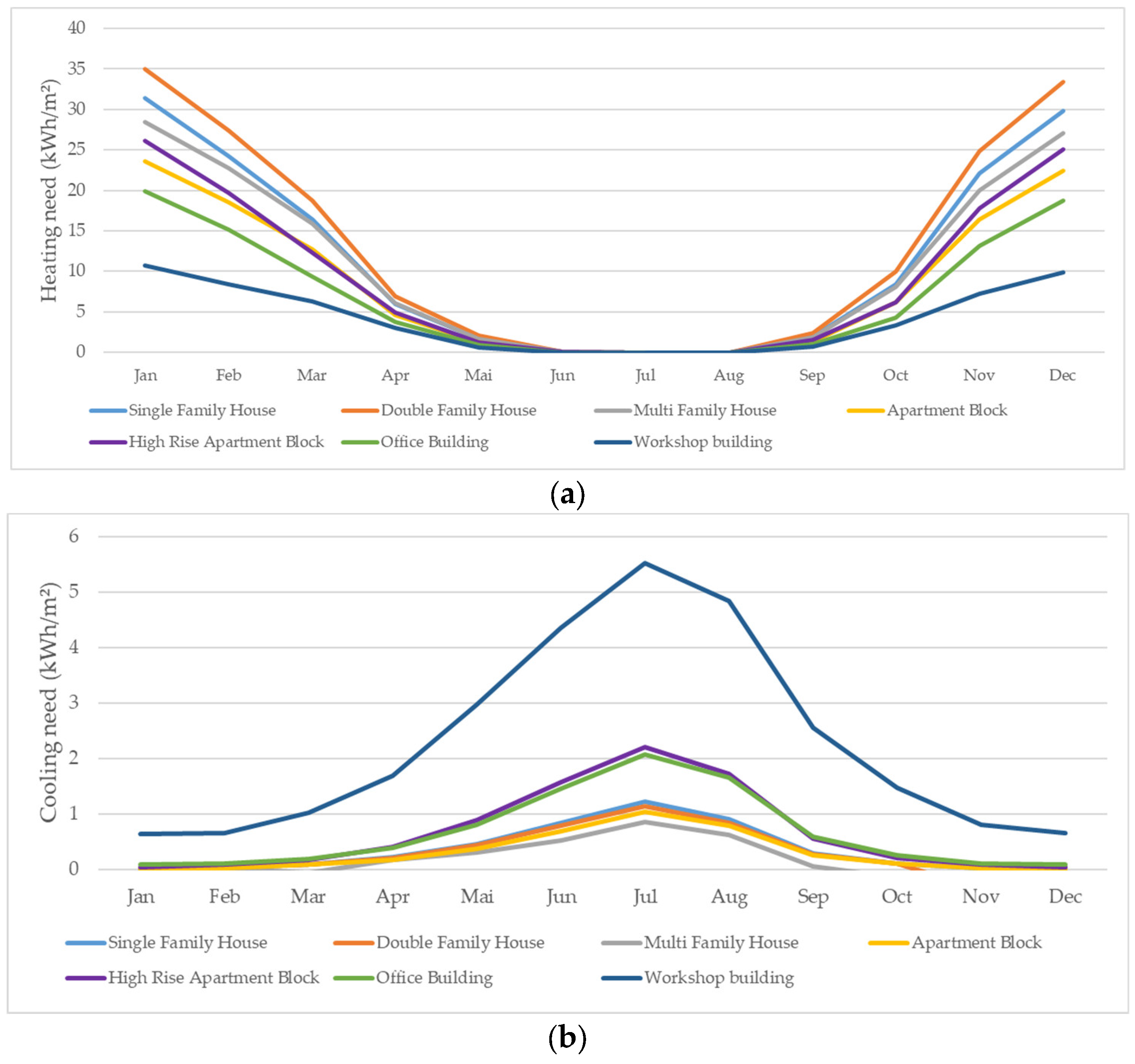
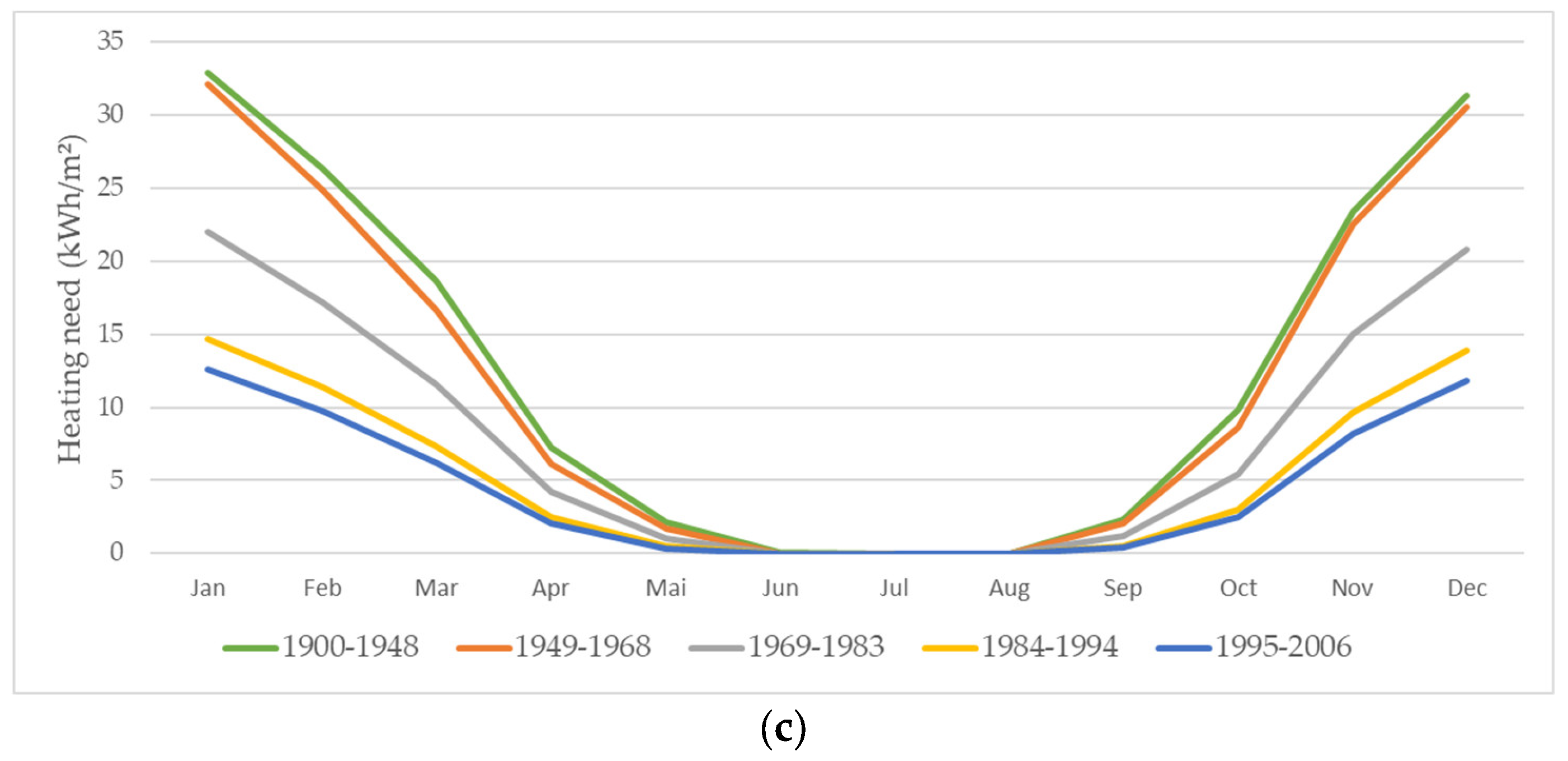
All these calculation steps and equations were programmatically implemented in the Eclipse environment using Python scripts, PostgreSQL and other related tools (see Section 2.3). Several scripts and functions were written in modular structure. They were divided into nine packages, which allowed inspection of intermediate results of the individual model components (Figure 3). The intermediate results and final outputs of the monthly cooling and heating energy needs were also saved as tables in the PostgreSQL/3DCityDB database from which automatized graphs were prepared. The databases were connected with QGIS to visualize the results in 2D and were also exported to ArcScene for visualization in a 3D environment.

4. Results

The model was applied on different numbers of building stocks (using both LOD1 and LOD2 data) in different Asian and European cities. This paper mainly explains the results obtained in the city of Karlsruhe, which is located in the southern Germany. The specific heating energy needs of the individual buildings ranges from about 15 to 510 kWh/m2a, depending on the characteristics and thermal behavior of the building as well as the local climate conditions (Figure 4). The cooling energy need is rather low (between 0 and 50 kWh/m2a), because of the moderately cooler climatic conditions in the study region.
The annual specific building energy needs were aggregated according to the building typologies (e.g., type and age) defined in this study. Figure 5 illustrates the total number of buildings (right y-axis) in each of the 33 typology and the aggregated heating and cooling energy needs (left y-axis). As expected, the heating needs are higher than the cooling needs in most of the building typologies (except the workshop buildings built after 1984). The highest specific heating energy needs are observed in double-family buildings built between 1900 and 1948 and the lowest in office buildings built between 1995 and 2006. In general, the older buildings have higher heating needs whereas the office and workshop buildings (independent of construction year) show higher cooling needs.
The monthly pattern of the heating and cooling energy needs varies among the seven building types (Figure 6a,b). The double family buildings tend to have higher specific heating needs throughout the heating period (October to April) than the other building types. Regarding cooling energy needs, office buildings and high-rise apartment blocks demonstrate similar patterns during cooling months (June to August). The other residential buildings show minimum cooling needs. The older buildings, as observed earlier, demonstrate higher specific heating energy needs than those of the recent buildings (Figure 6c).
The CityBEM monthly model was applied in several European and Asian cities, with varying numbers of buildings in both LOD1 and LOD2 data. The multiprocessing package of Python was exploited to improve the computational efficiency of handling of large 3D city models. The model proves very efficient and quick in displaying results. For example, in a typical virtual machine—a Linux Server for Python with 64 GB Ram, 12 GB used, 10 cores, HDD 8.5 GB free and a PostgreSQL Server for the DBs with 16 GB Ram, 3.5 GB used, 10 cores, HDD 44 GB free—it takes around 3 min to run on around 4300 LOD2 buildings, 8 min on 12000 LOD2 buildings, and 28 s on 600 LOD1 buildings.

5. Validation of Model

A comprehensive three-step validation of the monthly model was performed to justify its applicability and robustness. At first, a review of the comparative validation results obtained by the different studies implementing the ISO 13790 method was performed. Second, to ensure the correct implementation of the method in Python programming interface, the input values and corresponding results suggested in the Annex J of ISO document [8], have been considered in the CityBEM. Finally, the energy needs of an office and a residential building were validated with a dynamic simulation model in TRNSYS.

5.1. Validation with Other Studies

ISO developers have internally carried out error estimation and validation of the monthly methods. They concluded that the monthly calculation gives correct results on an annual basis, but the results for individual months close to the beginning and end of the heating and cooling season can have large relative errors [8], (Section 5.3). Recently, several studies performed validation of ISO methods with widely used dynamic simulation software such as TRNSYS or EnergyPlus. Kristensen and Petersen [13] found out that the monthly quasi-steady-state model predicts a lower monthly energy need for space heating and higher monthly energy need for cooling compared to the dynamic model. Zangheri, Armani [16] found that the simplified monthly method tends to over-estimate the energy needs for cooling, especially for office buildings located in a Mediterranean climate. The results obtained by Vollaro, Guattari [11] confirms that the monthly method tends to overestimate and underestimate of approximately 12% and 14% the cooling and heating energy demands respectively, compared to the results obtained from the dynamic simulation with TRNSYS. Kim, Yoon [12] carried out a deterministic and a stochastic comparison of simple hourly method with the EnergyPlus 6.0 software, with the inputs and boundary conditions for both approaches as close to each other as possible. They found that in the deterministic method, ISO 13790 predicts less annual heating and cooling energy demands than EnergyPlus. In the stochastic approach, EnergyPlus showed higher stochastic robustness than ISO 13790. However, Vartieres, Berescu [18] found that the yearly cooling need obtained with the monthly method is almost three times higher than that of TRNSYS. From May to October, the predicted cooling demands by ISO 13790 are smaller than EnergyPlus ones, while in the other months the predicted cooling demands are larger than EnergyPlus [12]. Earlier Kokogiannakis, Strachan [14] confirmed that the monthly method demonstrates higher cooling needs than the other methods. The EU study in the ENTRANZE project concluded that heating needs in ISO monthly and hourly are in line with EnergyPlus but the cooling needs are different in some climatic conditions [16].
Therefore, most of the studies found that the ISO method predicts less heating and more cooling needs, compared to the dynamic simulation software. CityBEM also shows similar patterns of cooling and heating needs.

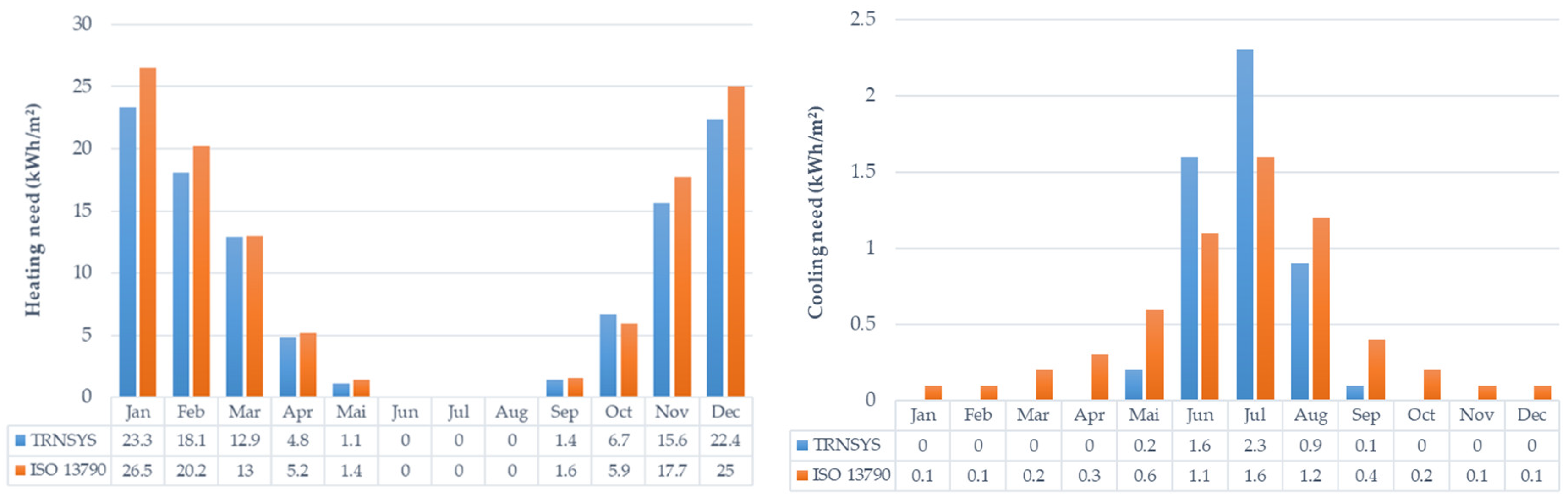
5.2. Validation with ISO 13790 Reference

In order to validate the proper implementation of ISO 13790 method, e.g., use of the model equations, the ISO authors have given some exemplary input data and corresponding results in the Annex J of the document [8]. Therefore, the robust implementation of the CityBEM model was tested using exactly the same input values as suggested. A test case consisting of an office building room with only one external wall facing west was considered. Other specific assumptions and simplifications (according to the suggestions) were made for the thermal heat flows and heat gains coefficients calculations. The monthly results obtained by the CityBEM exactly match with the annex results. This justifies the proper implementation of the ISO method in CityBEM.

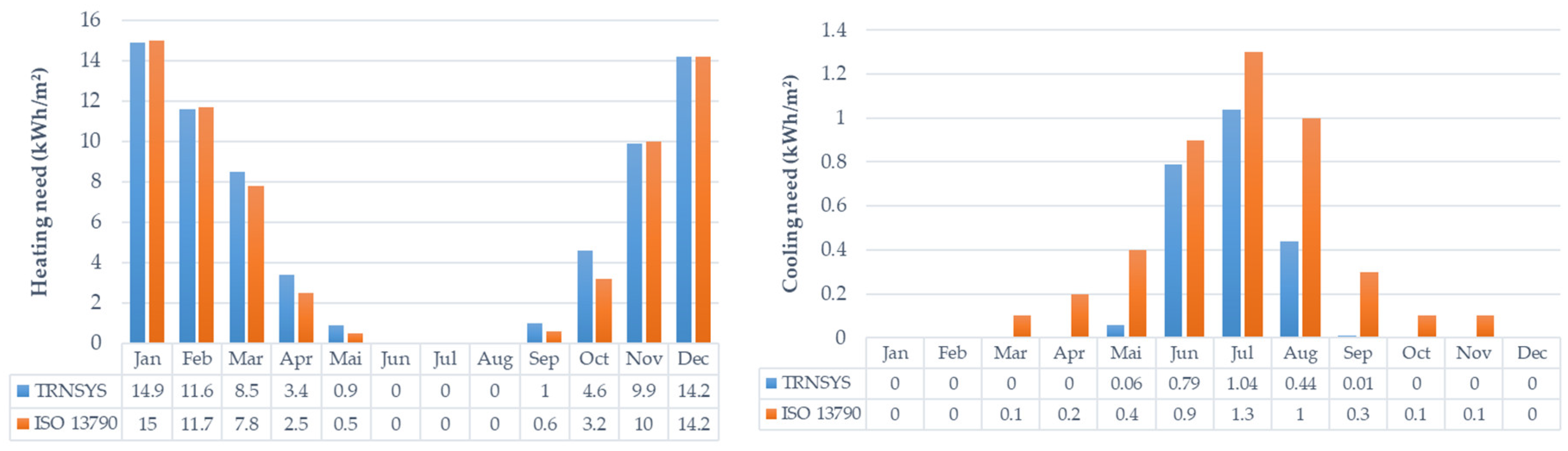
5.3. Validation with TRNSYS
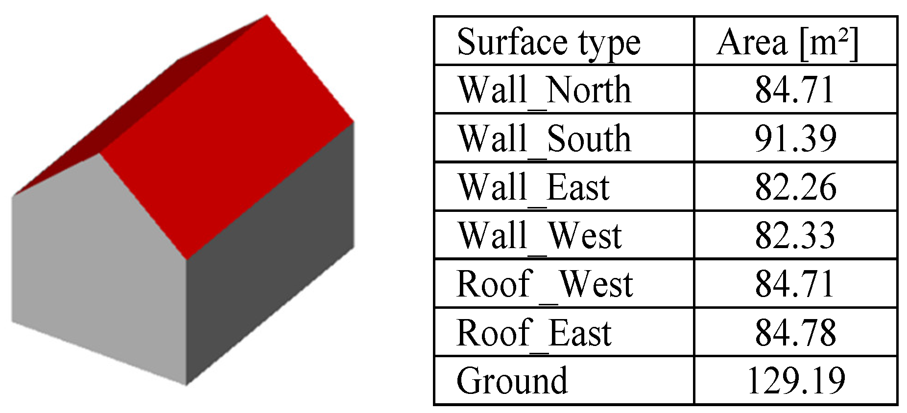
The dynamic simulation software TRNSYS was used to validate the results of the cooling and heating energy needs obtained by the CityBEM. TRNSYS was used to simulate the behaviour of the transient system (http://www.trnsys.com) and the simulations were focused on assessing the performance of thermal and electrical energy systems. TRNSYS cannot perform simulations on multiple buildings at a time, so two individual buildings, e.g., an office (built in 1975) and a residential building (built in 1985) in Karlsruhe were validated separately, with the same input data and assumptions as chosen in the CityBEM model.

5.3.1. Input Data

Several inputs are required in TRNSYS. At first, the two buildings were extracted from the CityGML dataset to calculate the building geometries, e.g., surface area of walls, roofs, etc. (Figure 7).
Then, the building attributes and thermal characteristics (e.g., surfaces areas, thickness and composition of walls, roof and ground layers, etc.) were given as inputs in TRNSYS. Calculation of internal gains were different in both models, therefore, careful attention has been given to ensure the same input of heat gains in both models. For this reason, the internal gain was set considering the table from ISO 7730 as suggested in TRNSYS. Then, the scale was adjusted by considering the monthly aggregated values of the internal heat gains in order to ensure exactly the same inputs in both TRNSYS and CityBEM.
Other parameters such as infiltration, ventilation, etc. were also considered identical in both models. The same Meteonorm weather data (wind speed, average temperature data) was given as an input. However, the TRNSYS software itself calculates the solar gains by the solar radiation model internally. An overview of the input datasets in TRNSYS software is given in Table 2.

5.3.2. Assumptions

Several assumptions were made to validate the CityBEM results with the TRNSYS:
  • Consideration of shading factors: In calculating solar gains in the CityBEM model, several factors such as, shading reduction factor for external obstacles (for the effective solar collection on the areas of surfaces), and form factor between the building element and the sky were considered. Nevertheless, the irradiation data obtained from PLANTING solar irradiance model already takes into account shading from external obstacles. Therefore, no shading reduction factor was considered in modelling solar gains in TRNSYS.
  • Averaging internal heat flow: In the method proposed by TABULA project (http://episcope.eu/iee-project/tabula), the internal heat flow is equal to 3 W/m2 for every building type. In the example of ISO (Annex J), it is 20 W/m2 from 8 a.m. to 6 p.m. So, the time average internal heat flow of 8 W/m2 (≈ 0.416 × 20) was considered in both approaches. This value refers to specific heat gains averaged for a day.
  • Introducing time reduction factors: Continuous cooling or heating is unrealistic. In order to make a good comparison, the scheduling factors in TRNSYS and in the CityBEM model were defined appropriately by introducing a time reduction factor.

5.3.3. Validation Results

Considering all the inputs and assumptions, the ISO 13790 based results (obtained by CityBEM model) of the heating and cooling energy needs of the residential (built in 1985) and office buildings (built in 1975) were validated with that of TRNSYS. Figure 8 and Figure 9 illustrate the comparative simulation results of the office building and the residential building, respectively.
For both of the buildings, the order of magnitude and the curve profiles are similar during the cooling and/or heating period in the TRNSYS simulation and the ISO based CityBEM model. The specific heating energy need obtained from the model is very similar to the TRNSYS simulation in different months. The relative error of the yearly heating is between 5% and 10%. Therefore, the implemented CityBEM monthly model seems to be robust for heating. Concerning cooling energy need, the results obtained by both approaches are quite different. The relative error of the yearly cooling goes from 18% to 80%. The differences or the uncertainties of the ISO monthly result may lie in the case study region of Karlsruhe, which requires rarely any cooling energy in the summer months. Similar patterns were also observed by Reference [14]. Therefore, it is essential to validate the cooling need in other regions where air conditioning is widely used.

6. Sensitivity Analyses

Sensitivity analyses try to quantify how the different influencing factors related to geometric characteristics relevant to the 3D city models, and future climate scenarios, affect the monthly building heating and cooling energy needs at an urban scale. In this regard, at first, the applicability of such datasets were tested. Then, different sensitivity analysis approaches and associated assumptions were reviewed to identify a suitable method for the monthly building energy model. To process the large data sets, the calculation process was automated through Python scripts, 3DCityDB and PostgreSQL databases. Finally, the results were analyzed and visualized in different graphs and thematic 3D buildings.
Two sets of sensitivity analyses, e.g., parameter sensitivity and climate sensitivity were performed in this study. In both cases, the results were evaluated against the results obtained in the reference scenarios (Figure 10).

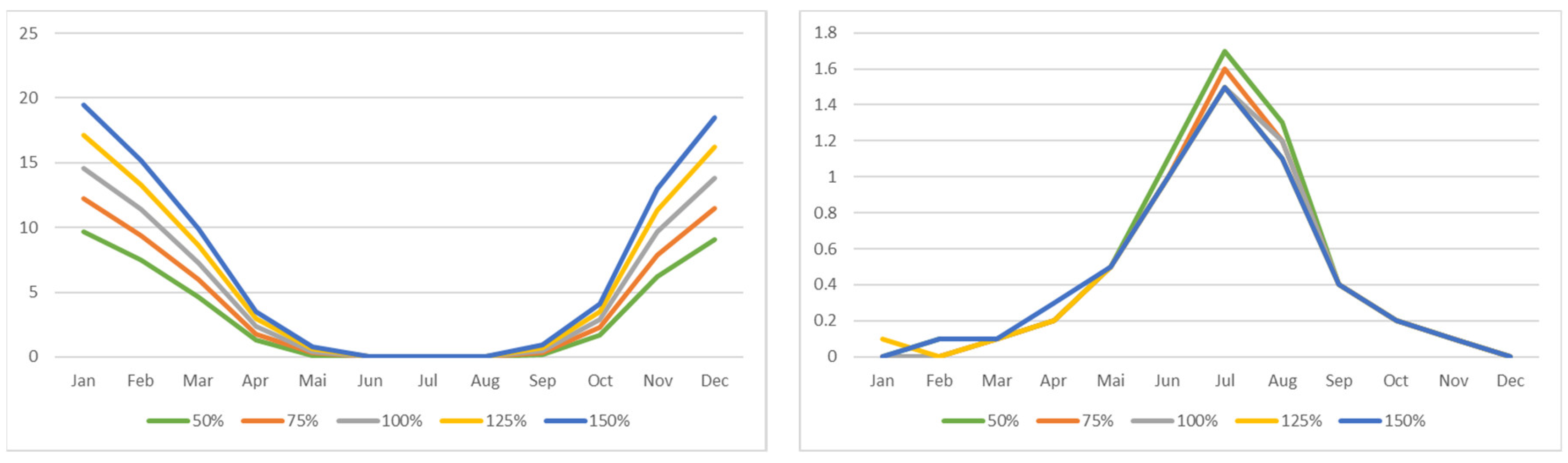
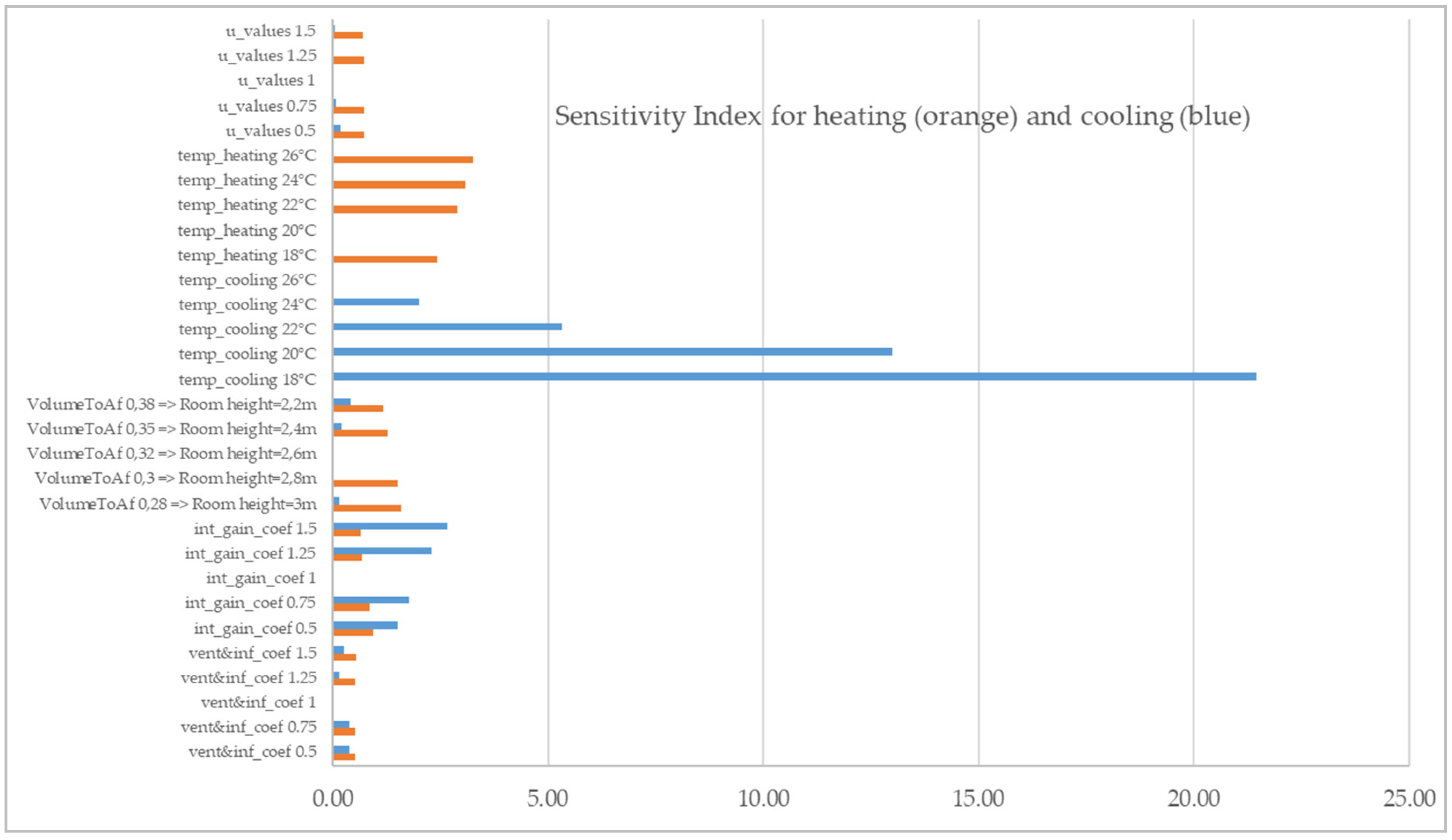
6.1. Parameter Sensitivity

Parameter sensitivity was performed by choosing a range of uncertain input parameters, such as U-values, volume to floor area ratios, ventilation coefficients, internal heat gains and set point temperatures for heating and cooling. They were carefully derived from the building ordinance guidelines to ensure realistic assumptions. However, the spread of the different input parameters were very different, therefore, they were carefully set (individually) to avoid any bias that may occur. Finally, they were applied in the previously mentioned residential building built in 1985, located in the city of Karlsruhe in Germany. Table 3 explains the input parameters chosen for the sensitivity analysis of the applied model. Each parameter value was changed one at a time to record the monthly heating and cooling energy needs (see Appendix A).
U-values of ground, roof, wall and window were changed by 50%, 75%, 125% and 150%, compared to the reference values (100%) to record the monthly variation of specific heating and cooling energy needs. Such variations do not have a significant impact on the cooling energy needs but have impacts on the heating energy needs during the winter months (Figure 11).
A volume to floor area coefficient of 0.32 (equivalent to 2.6 m of room height and assuming a factor 1.2 between the original area and floor area) was considered as reference value. For sensitivity analysis, room heights were varied from 2.2 to 3 m to understand their impact on modelling results. They have a minor impact on modelling heating and cooling needs. Ventilation and infiltration coefficients were changed by 50%, 75%, 125% and 150%, compared to the reference values (100%). They have significant impact both on the heating and cooling energy needs in the winter and summer months. Internal heat gains were also varied by 50%, 75%, 125% and 150%, compared to the reference values (100%). The impact was more significant in cooling energy needs especially during the summer months than in the heating energy needs in the winter months.
Finally, the set point temperature for both heating and cooling were varied by 18, 20, 22, 24, and 26 °C to quantify their impact. Heating set point temperatures have proportionate impacts on the heating energy needs, but the cooling set point temperatures resulted in disproportionate cooling energy needs (Figure 12).

6.2. Derivation of Sensitivity Index

The sensitivity index (SI) was prepared following the local method as described in Reference [32], (Table 1). It expresses the output elasticity of variation around the mean output value as percentage change in output, per percentage change in input. It produces dimensionless coefficients to rank the most important model parameters.
SI = % change in output/% change in input
The set point temperature was found to be the most influencing parameter in assessing both heating and cooling energy needs of the reference building. The cooling set point temperature of 18 °C has the maximum index value of 21.44, whereas the heating set point temperature of 26 °C has a maximum index value of 3.26 (Figure 13). For annual heating energy needs, room height and internal heat gains are also found to have significant impacts; whereas for cooling, internal heat gain has significant impacts.

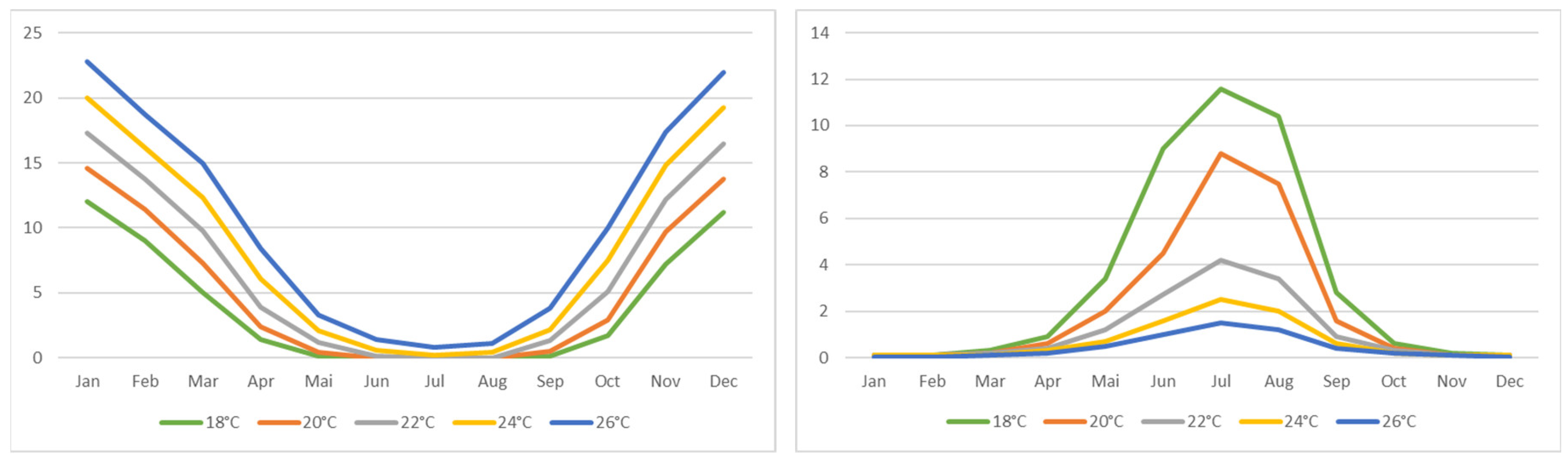
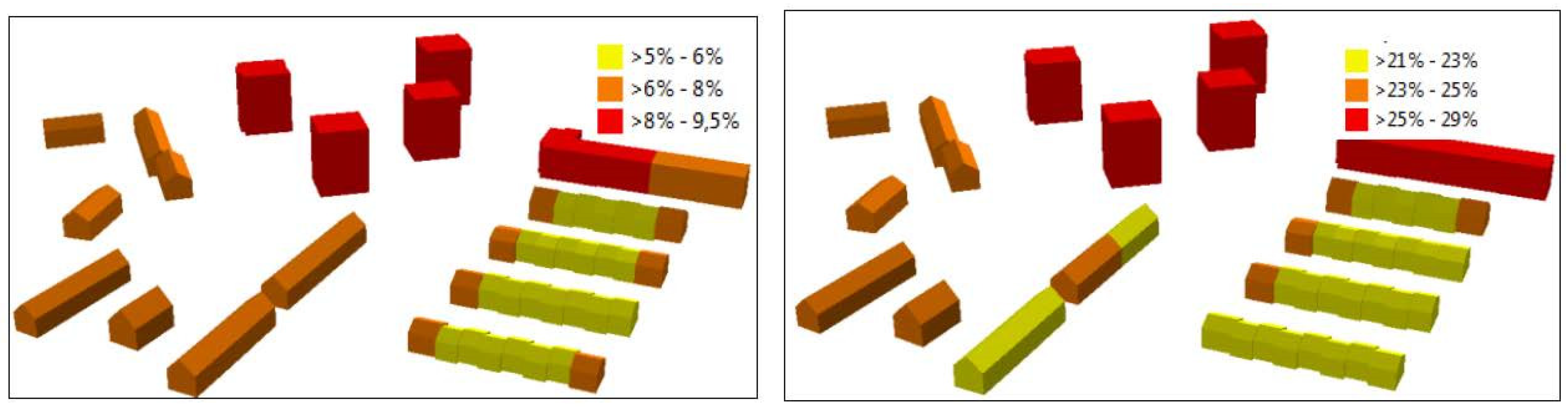
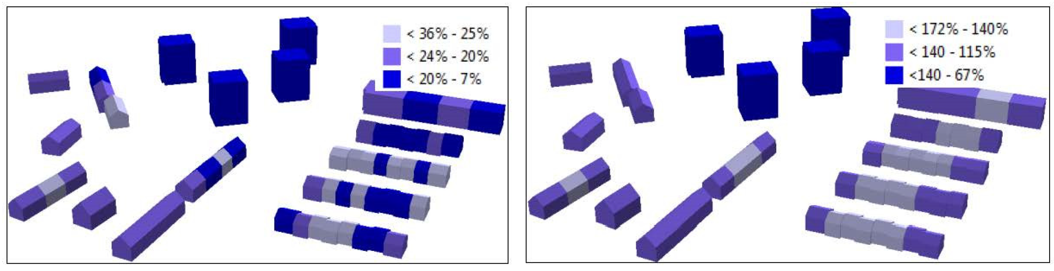
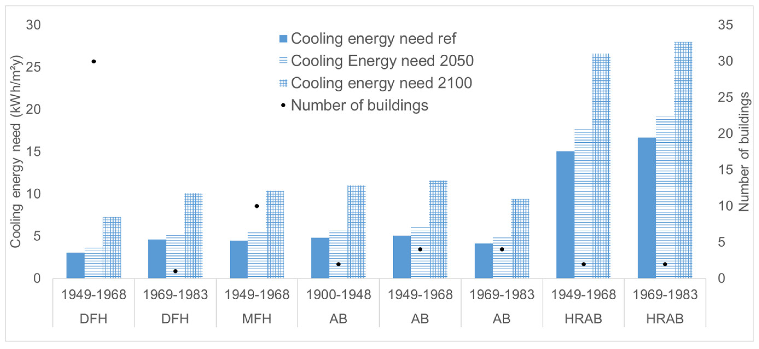
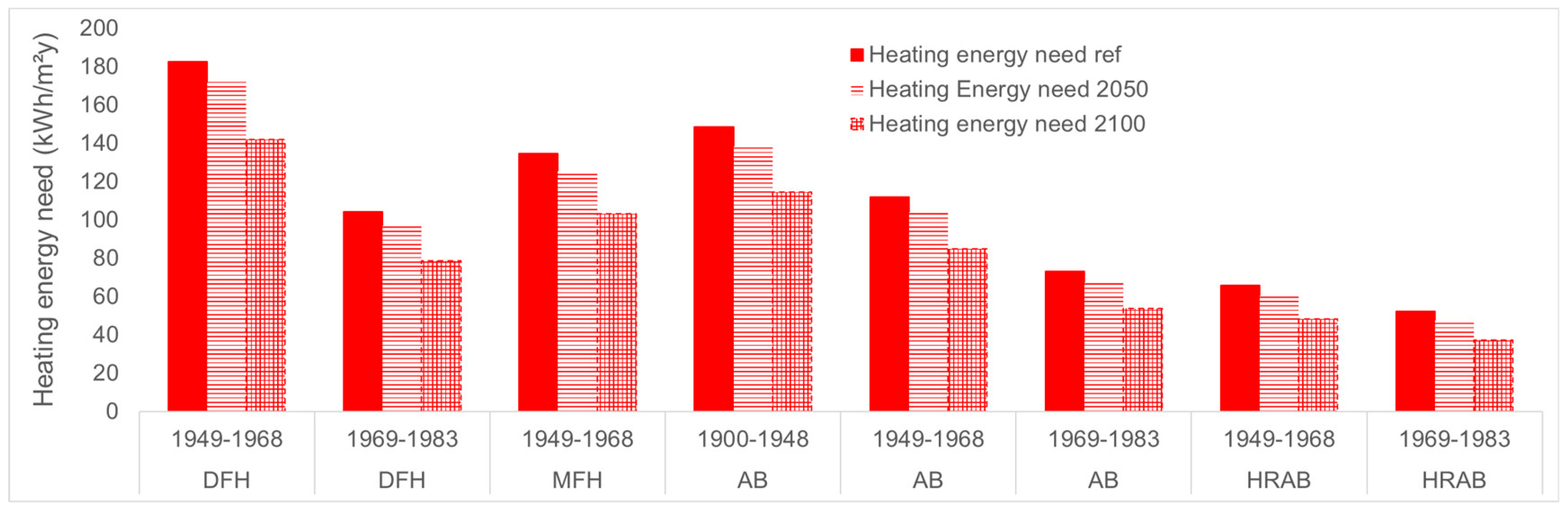
6.3. Climate Sensitivity

Sensitivity of future climate conditions were tested with the LOD2 CityGML data of the selected 95 buildings—having four building types (double-family house, multi-family house, apartment block, and high-rise apartment block) and three age categories (1900–1948, 1949–1968, and 1969–1983)—in an urban district in Karlsruhe. In this regard, IPCC A2 climate scenarios for 2050 and 2100 were extracted from the Meteonorm 7 climate dataset. The Meteonorm software itself does not calculate any climate scenarios. The CityBEM was run on these datasets (assuming all other input parameters were constant; they were chosen according to Table 1) to compare the results with the reference climate scenario, which represents a typical meteorological year.
The results show that the heating energy needs in all the buildings in this district in 2050 and 2100 will decrease, while the cooling energy needs will increase significantly. Depending on the building typology (age, type), the heating energy needs of the different buildings decrease from 5 to 9.5% in 2050, and from 21 to 29% in 2100 (Figure 14). In the case of cooling energy need, it will increase from 7 to 36% in 2050 and from 67 to 172% in 2100 (Figure 15).
The annual specific building energy needs were aggregated according to the eight building typologies (e.g., type and age) defined in this study. Figure 16 and Figure 17 illustrate specific annual energy needs (left y-axis) and the total number of buildings (right y-axis) in each of these corresponding typologies (x-axis). As expected, the heating need in the reference year is higher than the cooling needs in all the building typologies. The energy need will change proportionately in all typologies; except for the high-rise apartment buildings (HRAB), where a significant increase of cooling energy need is foreseen.

6.4. Discussion

The sensitivity index using the local method reveals that the set point temperature has the most significant impact on the modelling results. So far, the results support the findings of Kim et al. [12]. In quantifying the impact of climate change on the energy needs in a district, it was shown that the future climate scenarios significantly reduced heating energy needs and increase the cooling energy needs for the discussed geographical area. Impacts will vary depending on building typologies. Therefore, this research can indirectly support policy makers in promoting more resilient urban forms (i.e., typologies) to reduce consequences of climate changes on future energy needs at a city scale.
The discussion of general scenarios of the building sector goes beyond the scope of this paper. Yet, the results presented here for the purpose of a sensitivity analysis clearly show emerging problems in many growing economies worldwide. While increased building performance and more efficient technical systems can reduce the energy needs of buildings, a number of factors is likely going to overcompensate efficiency gains. Increase in the space per capita as well as higher comfort requirements (i.e., lower temperatures for cooling case) can be assumed to be accompanied by economic growth. In combination with changing climate conditions, the results of the sensitivity analyses indicate that building technologies will not be sufficient to overcome the harmful environmental impact of our buildings. In order to reach international climate goals and minimize the most serious impacts, technology solutions do not suffice. The presented results hint at the urgent need to address both technical as well as non-technical measures that can help to reduce the energy needs of buildings and thus their environmental impacts. Savings from advances in technology alone are likely to be overcompensated by increases due to factors connected to individual lifestyles and societal norms.

7. Conclusions

In this study, the CityBEM monthly model was developed through an open source implementation of the ISO 13790:2008 method to calculate monthly heating and cooling energy need for a large number of building stocks in a neighborhood or city. It was based on the 3D city models of the CityGML format and other required input parameters, such as the building geometry, typology and energy characteristics. The model was applied in several urban districts with varying numbers of buildings stocks, using both LOD1 and LOD2 datasets. The robustness of the model was also tested using a three-step validation approach. The model itself and the sensitivity analyses can help to determine the potential of energy efficiency in the buildings to reduce harmful environmental impacts. It can help urban decision makers to perform city or district wide analysis of the building energy need and to prepare different renovation plans, which finally will help to enhance the livability of the city and quality of life of the citizens.
The monthly ISO method has several limitations, which have also been identified in other studies. It is based on steady-state conditions, the variation of parameters such as heat flows and heat transfer coefficient depends on the external temperature which is set to a constant value for each month [11]. Vartieres et al. [18] concluded that assuming constant temperature with fresh air introduced cooling loads during transition months, when outdoor airflow could reduce the temperature. The ventilation airflow supplied from the outside with a smaller averaged external temperature gives heat losses by ventilation even during summer. Moreover, the users and their behavior play an important role in calculating building energy needs. It was difficult to collect such exact data for each building. Regarding handling of 3D data, we observed geometrical and topological errors in the CityGML dataset, which could not be completely imported into the PostgreSQL database, resulting in exclusion of some buildings in the analysis. Nouvel et al. [27] and Agugiaro [28] also explained such uncertainties, e.g., geometrical precision, thermal building parameters estimation, etc., of the 3D city models. Finally, each building was modelled as single zone in this study. With the availability of more detailed building information, e.g., LOD3 or LOD4 city models, buildings can be modelled as multi-zones. Such city models will also facilitate exact calculation of window or chimney areas and thus improve the modelling results.
The ISO monthly method (and therefore the CityBEM model) can be further improved. For example, Vartieres et al. [18] suggested introduction of a variable supply air change, by dividing each month into two intervals. Moreover, in calibration of dynamic parameters, different studies carried out a comparison between dynamic simulations and the monthly methods, and they all agree that the loss utilization factor formula is correct in its general equation, and that the numerical coefficient should be better defined for each specific case study.
Several limitations can also be observed in sensitivity analyses. For instance, long-term prediction of climate change is subject to uncertainties and the prediction of different climate variables may not be accurate. They have direct impacts on modelling results. The cooling energy modelling results are performed in a German city, where such energy need is not very high. While the presented research aimed at studying the sensitivity of the model, more comprehensive studies could be conducted using the selected approach to perform impact analysis in different world regions based on the existing urban form. For such studies, climate regions with high cooling energy needs are obvious focus areas. The presented approach could therefore in the future be used to study the sensitivities of the physical shape of the building in the context of urban form to quantify impacts on calculated heating and cooling energy needs.
The model can, however, be further improved in future. The energy needs for heating and cooling can be used as an input for the energy balance of the heating and cooling systems and ventilation system in order to calculate the energy use. Hourly and seasonal energy can also be calculated. In this regard, the CityBEM monthly model can also be validated with the hourly method by aggregating the hourly values into months and years. The sensitivity of some other critical model input parameters (e.g., heat capacity, building orientation, etc.) can also be performed in future. Building energy saving potential and further refurbishment priorities/scenarios can be simulated to identify more applications of the model. Some micro and macroclimate parameters relevant to the district scale, such as shading from the neighboring buildings, are modelled in calculating solar gains. Some other parameters, such as effects of trees, evaporation, the urban heat island effects, and waste heat of building surfaces were not modelled. They can be incorporated in modelling the energy needs at an urban scale.

Author Contributions

S.M.M. envisioned and wrote the article with a support from S.P. and A.K.; S.P. performed the initial coding and analyses of the model, with the support of S.M.M and A.K. The article was improved by the contributions of all the co-authors at various stages of the analysis and writing process.

Funding

This research received no external funding.

Acknowledgments

We are grateful to the city of Karlsruhe for providing the 3D city models as well as EDF R&D and EIFER for internal funding the research. We would like to thank Hicham Bidah and Alexander Simons for their initial support in application development. Finally, our sincere gratitude extends to the editors and three anonymous referees for their insightful comments, which helped us to improve the manuscript.

Conflicts of Interest

The authors declare no conflict of interest.

Appendix A. Results of Parameter Sensitivity Analyses

Parameters Values/MonthMonthly Heating Energy Needs (kWh/m²)Monthly Cooling Energy Needs (kWh/m²)Total Annual Heating NeedsTotal Annual Cooling Needs
JanFebMarAprMayJunJulAugSepOctNovDecJanFebMarAprMayJunJulAugSepOctNovDec
vent&inf_coef 0.511.18.55.21.50.20000.227.110.500.10.10.30.61.21.81.40.50.20046.36.2
vent&inf_coef 0.7512.89.96.320.30000.42.58.412.20.10.10.10.20.51.11.61.30.40.20.1054.85.7
vent&inf_coef 114.611.47.32.40.40000.52.99.713.8000.10.20.511.51.20.40.20.10635.2
vent&inf_coef 1.2516.412.88.32.80.60000.73.410.915.500.10.10.20.50.91.41.10.40.20.1071.45
vent&inf_coef 1.518.114.29.43.30.70000.8412.217.20.10.10.10.20.40.91.310.30.10079.94.5
int_gain_coef 0.519.515.711.44.90.800016.414.118.70000.10.10.30.40.30.100092.51.3
int_gain_coef 0.751713.49.23.30.60000.74.511.716.20000.10.30.60.90.70.20.10076.62.9
int_gain_coef 114.611.47.32.40.40000.52.99.713.8000.10.20.511.51.20.40.20.10635.2
int_gain_coef 1.2512.59.65.620.30000.42.37.811.70.10.10.20.40.81.52.21.80.60.30.10.152.28.2
int_gain_coef 1.510.57.94.21.70.20000.326.29.80.20.20.30.61.22.232.510.50.20.242.812.1
VolumeToAf 0.28 => Room height=3m17.313.58.730.60000.73.711.616.400.10.10.20.511.41.10.40.20.1075.55.1
VolumeToAf 0.3 => Room height=2.8m15.912.482.70.50000.63.310.515.100.10.10.20.511.51.10.40.20.10695.2
VolumeToAf 0.32 => Room height=2.6m14.611.47.32.40.40000.52.99.713.8000.10.20.511.51.20.40.20.10635.2
VolumeToAf 0.35 => Room height=2.4m1310.16.420.30000.42.58.512.300.10.10.20.511.61.20.40.20055.55.3
VolumeToAf 0.38 => Room height=2.2m11.695.71.70.20000.32.27.51100.10.10.20.51.11.61.30.40.20.1049.25.6
temp_cooling 18°C14.611.47.32.40.40000.52.99.713.80.10.10.30.93.4911.610.42.80.60.20.16339.5
temp_cooling 20°C14.611.47.32.40.40000.52.99.713.80.10.10.20.624.58.87.51.60.40.10.16326
temp_cooling 22°C14.611.47.32.40.40000.52.99.713.80.10.10.20.41.22.74.23.40.90.30.10.16313.7
temp_cooling 24°C14.611.47.32.40.40000.52.99.713.80.10.10.10.30.71.62.520.60.20.10.1638.4
temp_cooling 26°C14.611.47.32.40.40000.52.99.713.8000.10.20.511.51.20.40.20.10635.2
temp_heating 18°C12951.40.10000.11.77.211.2000.10.20.511.51.20.40.20.1047.75.2
temp_heating 20°C14.611.47.32.40.40000.52.99.713.8000.10.20.511.51.20.40.20.10635.2
temp_heating 22°C17.313.89.83.91.20.1001.35.112.216.5000.10.20.511.51.20.40.20.1081.25.2
temp_heating 24°C2016.212.36.12.10.60.20.42.27.514.819.3000.10.20.511.51.20.40.20.10101.75.2
temp_heating 26°C22.818.7158.43.31.40.81.13.81017.422000.10.20.511.51.20.40.20.10124.75.2
u_values 0.59.77.54.61.30.10000.21.76.29.100.10.10.20.51.11.71.30.40.20.1040.45.7
u_values 0.7512.29.461.80.30000.32.37.911.5000.10.20.511.61.20.40.20.1051.75.3
u_values 114.611.47.32.40.40000.52.99.713.8000.10.20.511.51.20.40.20.10635.2
u_values 1.2517.113.38.630.60000.73.511.316.20.100.10.20.511.51.10.40.20.1074.35.2
u_values 1.519.515.29.93.50.80000.94.11318.500.10.10.30.511.51.10.40.20.1085.45.3

References

  1. Swan, L.G.; Ugursal, V.I. Modeling of end-use energy consumption in the residential sector: A review of modeling techniques. Renew. Sustain. Energy Rev. 2009, 13, 1819–1835. [Google Scholar] [CrossRef]
  2. Nouvel, R.; Mastrucci, A.; Leopold, U.; Baume, O.; Coors, V.; Eicker, U. Combining gis-based statistical and engineering urban heat consumption models: Towards a new framework for multi-scale policy support. Energy Build. 2015, 107, 204–212. [Google Scholar] [CrossRef]
  3. Bahu, J.-M.; Koch, A.; Kremers, E.; Murshed, S.M. Towards a 3D spatial urban energy modelling approach. Int. J. 3-D Inf. Model. (IJ3DIM) 2014, 3, 1–16. [Google Scholar] [CrossRef]
  4. Koch, E.A. Continuous Simulation for Urban energy Planning Based on a Non-Linear Data-Driven Modelling Approach; Karlsruher Instituts für Technologie: Karlsruhe, Germany, 2016. [Google Scholar]
  5. Chalal, M.L.; Benachir, M.; White, M.; Shrahily, R. Energy planning and forecasting approaches for supporting physical improvement strategies in the building sector: A review. Renew. Sustain. Energy Rev. 2016, 64, 761–776. [Google Scholar] [CrossRef] [Green Version]
  6. Reinhart, C.F.; Davila, C.C. Urban building energy modeling–A review of a nascent field. Build. Environ. 2016, 97, 196–202. [Google Scholar] [CrossRef]
  7. Mendes, G.; Ioakimidis, C.; Ferrão, P. On the planning and analysis of Integrated Community Energy Systems: A review and survey of available tools. Renew. Sustain. Energy Rev. 2011, 15, 4836–4854. [Google Scholar] [CrossRef]
  8. ISO. Energy performance of buildings—Calculation of energy use for space heating and cooling. In ISO 13790:2008(E); International Organization for Standardization: Geneva, Switzerland, 2008; p. 162. [Google Scholar]
  9. Attia, S.; Ana Muresan, A. Romanian Standards for Energy Performance in Buildings Translation of the Romanian Standards for Energy Performance in Buildings; Sustainable Buildings Design Lab: Liege, Belgium, 2015; p. 61. [Google Scholar]
  10. Kwak, H.-J.; Jo, J.-H.; Suh, S.-J. Evaluation of the reference numerical parameters of the monthly method in ISO 13790 considering s/v ratio. Sustainability 2015, 7, 767–781. [Google Scholar] [CrossRef]
  11. Vollaro, R.D.L.; Guattari, C.; Evangelisti, L.; Battista, G.; Carnielo, E.; Gori, P. Building energy performance analysis: A case study. Energy Build. 2014, 87, 87–94. [Google Scholar] [CrossRef]
  12. Kim, Y.-J.; Yoon, S.-H.; Park, C.-S. Stochastic comparison between simplified energy calculation and dynamic simulation. Energy Build. 2013, 64, 332–342. [Google Scholar] [CrossRef]
  13. Kristensen, M.H.; Petersen, S. Choosing the appropriate sensitivity analysis method for building energy model-based investigations. Energy Build. 2016, 130, 166–176. [Google Scholar] [CrossRef]
  14. Kokogiannakis, G.; Strachan, P.; Clarke, J. Comparison of the simplified methods of the ISO 13790 standard and detailed modelling programs in a regulatory context. J. Build. Perform. Simul. 2008, 1, 209–219. [Google Scholar] [CrossRef] [Green Version]
  15. Corrado, V.; Fabrizio, E. Assessment of building cooling energy need through a quasi-steady state model: Simplified correlation for gain-loss mismatch. Energy Build. 2007, 39, 569–579. [Google Scholar] [CrossRef]
  16. Zangheri, P.; Armani, R.; Pietrobon, M.; Pagliano, L.; Boneta, M.F.; Müller, A. Heating and Cooling Energy Demand and Loads for Building Types in Different Countries of the EU; Report in the Frame of the EU Project ENTRANZE; Politecnico di Milano: Milan, Italy, 2014. [Google Scholar]
  17. Sirén, K.; Hasan, A. Comparison of Two Calculation Methods Used to Estimate Cooling Energy Demand and Indoor Summer Temperatures. In Proceedings of the Clima 2007 Well-Being Indoors, Helsinki, Finland, 10–14 June 2007. [Google Scholar]
  18. Vartieres, A.; Berescu, A.; Damian, A. Energy demand for cooling an office building. In Proceedings of the 11th International Conference on Environment, Ecosystems and Development, Brasov, Romania, 1–3 June 2013; pp. 132–135. [Google Scholar]
  19. Petersen, S.; Svendsen, S. Method and simulation program informed decisions in the early stages of building design. Energy Build. 2010, 42, 1113–1119. [Google Scholar] [CrossRef]
  20. Sun, Y. Sensitivity analysis of macro-parameters in the system design of net zero energy building. Energy Build. 2015, 86, 464–477. [Google Scholar] [CrossRef]
  21. Heiselberg, P.; Brohus, H.; Hesselholt, A.; Rasmussen, H.; Seinre, E.; Thomas, S. Application of sensitivity analysis in design of sustainable buildings. Renew. Energy 2009, 34, 2030–2036. [Google Scholar] [CrossRef] [Green Version]
  22. Spitz, C.; Mora, L.; Wurtz, E.; Jay, A. Practical application of uncertainty analysis and sensitivity analysis on an experimental house. Energy Build. 2012, 55, 459–470. [Google Scholar] [CrossRef]
  23. Lomas, K.J.; Eppel, H. Sensitivity analysis techniques for building thermal simulation programs. Energy Build. 1992, 19, 21–44. [Google Scholar] [CrossRef]
  24. OGC. OGC City Geography Markup Language (Citygml) Encoding Standard 2.0.0; Open Geospatial Consortium: Wayland, MA, USA, 2012; p. 344. [Google Scholar]
  25. Biljecki, F.; Stoter, J.; Ledoux, H.; Zlatanova, S.; Çöltekin, A. Applications of 3D city models: State of the art review. ISPRS Int. J. Geo-Inf. 2015, 4, 2842–2889. [Google Scholar] [CrossRef] [Green Version]
  26. Eicker, U.; Nouvel, R.; Schulte, C.; Schumacher, J.; Coors, V. 3D Stadtmodelle für Die Wärmebedarfberechnung. In Proceedings of the Fourth German-Austrian IBPSA Conference, Berlin, Germany, 26–28 September 2012. [Google Scholar]
  27. Nouvel, R.; Schulte, C.; Eicker, U.; Pietruschka, D.; Coors, V. Citygml-based 3D city model for energy diagnostics and urban energy policy supports. In Proceedings of the 13th Conference of International Building Performance Simulation Association, Chambéry, France, 26–28 August 2013. [Google Scholar]
  28. Agugiaro, G. Energy planning tools and CityGML-based 3D virtual city models: Experiences from Trento (Italy). Appl. Geomat. 2016, 8, 41–56. [Google Scholar] [CrossRef]
  29. Meteonorm. Meteonorm Global Meteorological Database—Version 7 Software and Data for Engineers, Planners and Education, 7th ed.; Meteotest AG: Bern, Switzerland, 2018. [Google Scholar]
  30. Murshed, S.M.; Lindsay, A.; Picard, S.; Simons, A. PLANTING: Computing high spatio-temporal resolutions of photovoltaic potential of 3D city models. In Geospatial Technologies for All, Lecture Notes in Geoinformation and Cartography; Mansourian, A., Pilesjö, P., Harrie, L., van Lammere, R., Eds.; Springer International Publishing AG: Cham, Switzerland, 2018. [Google Scholar]
  31. Murshed, S.M.; Simons, A.; Lindsay, A.; Picard, S.; De Pin, C. Evaluation of Two Solar Radiation Algorithms on 3D City Models for Calculating Photovoltaic Potential. In Proceedings of the 4th International Conference on Geographical Information Systems Theory, Applications and Management (GISTAM 2018), Funchal, Madeira, Portugal, 17–19 March 2018; SCITEPRESS—Science and Technology Publications, Lda: Setúbal, Portugal, 2018. [Google Scholar]
  32. Lam, J.C.; Hui, S.C. Sensitivity analysis of energy performance of office buildings. Build. Environ. 1996, 31, 27–39. [Google Scholar] [CrossRef]
Figure 1. Overall research methodology of this study.
Ijgi 07 00447 g001
Figure 2. Overview of different software, tools and datasets required to implement CityBEM model (modified after Reference [30]).
Ijgi 07 00447 g002
Figure 3. Implementation steps of the CityBEM model: Different input data, related software packages and the tables created in the databases.
Ijgi 07 00447 g003
Figure 4. Illustration of annual heating energy need (kWh/m2) in a district in the city of Karlsruhe in Germany.
Ijgi 07 00447 g004
Figure 5. Annual specific building heating and cooling energy needs in 33 building typologies and corresponding number of buildings in each typology (SFH = Single Family House, DFH = Double Family House, MFH = Multi Family House, AB = Apartment Block, HRAB = High Rise Apartment Block, OB = Office Building, WB = Workshop Building).
Ijgi 07 00447 g005
Figure 6. Monthly specific (a) heating and (b) cooling energy needs for seven building types and (c) heating energy needs for five building age classes.
Ijgi 07 00447 g006aIjgi 07 00447 g006b
Figure 7. The CityGML building extracted for simulation in TRNSYS (left) and corresponding geometric properties (right).
Ijgi 07 00447 g007
Figure 8. Comparison of energy simulation results obtained with TRNSYS and ISO-based CityBEM for an office building (1975).
Ijgi 07 00447 g008
Figure 9. Comparison of energy simulation results obtained with TRNSYS and ISO-based CityBEM for a residential building (1985).
Ijgi 07 00447 g009
Figure 10. Sensitivity analyses approach for the CityBEM monthly model.
Ijgi 07 00447 g010
Figure 11. Sensitivity of U-values on monthly energy needs for heating (left) and cooling (right).
Ijgi 07 00447 g011
Figure 12. Sensitivity of set point temperature on monthly energy needs for heating (left) and cooling (right).
Ijgi 07 00447 g012
Figure 13. Sensitivity indices for monthly heating and cooling energy needs considering the local method.
Ijgi 07 00447 g013
Figure 14. Decrease of annual heating energy needs in 2050 (left) and in 2100 (right), compared to the reference scenarios.
Ijgi 07 00447 g014
Figure 15. Increase of annual cooling energy needs in 2050 (left) and in 2100 (right), compared to the reference scenarios.
Ijgi 07 00447 g015
Figure 16. Impact of future climate change on specific cooling energy needs of different building typologies in an urban district in Karlsruhe.
Ijgi 07 00447 g016
Figure 17. Impact of future climate change on specific heating energy needs of different building typologies in an urban district in Karlsruhe.
Ijgi 07 00447 g017
Table 1. Required input data and corresponding sources for the CityBEM monthly model.
Input dataUnitSource
Building Geometry
Wall Northm2CityGML data
Wall Southm2CityGML data
Wall Eastm2CityGML data
Wall Westm2CityGML data
Volumem3CityGML data
Floor area/conditioned used aream2Calculated from EnEV 2015 and volume
Effective mass aream2Calculated from the floor area [8] pp. 66–68
Building Typology
Windows North% District Energy Concept Advisor 1
Windows South%District Energy Concept Advisor
Windows East%District Energy Concept Advisor
Windows West%District Energy Concept Advisor
U-value wallW/m2KIWU 2
U-value roofW/m2KIWU
U-value groundW/m2KIWU
U-value windowsW/m2KIWU
g-value windows-IWU
Thermal bridgesW/m2KIWU
Infiltration1/hIWU
Ventilation1/hIWU
Internal heat from occupantsW/m2IWU
Internal heat from appliancesW/m2IWU
Internal heat from lightingW/m2IWU
Climate Conditions
Monthly temperature of the external environment°CMeteonorm (TMY3)
Monthly wind speedm/sMeteonorm (TMY3)
Monthly solar irradianceW/m2Solar radiation model
1http://www.district-eca.de; 2Institut Wohnen und Umwelt GmbH (Institute for housing and environment, http://www.iwu.de).
Table 2. Input data of the residential and office building in the TRNSYS simulation software.
ParametersResidential BuildingOffice Building
Window area (m2)North4.47 (4.9%)9.27 (10.16%)
South11.19 (12.25%)8.34 (9.13%)
East5.54 (6.74%)10.08 (12.25%)
West5.54 (6.74%)11.39 (13.85%)
U values (W/m2k)Wall0.61.5
Roof0.41
Floor0.61.2
Window2.72.9
G value (-) 0.750.75
Thermal bridges (W/m2K) 0.10.15
Infiltration (h−1) 0.20.2
Ventilation (h−1) 0.50.5
Internal heat gains (W/m2) 19.424.7
Set-point temperature (°C)Heating2020
Cooling2626
Table 3. Range of sensitivities chosen for the input parameters.
Input Parameters for Sensitivity AnalysesReference ValuesRange of Sensitive Values Chosen
U-values of ground, roof, wall and window (W/m2K)10.5, 0.75, 1.25, 1.5
Volume to floor area ratio (1/m)0.32 (having room height 2.6 m)0.28, 0.30, 0.35, 0.38 (having room height 3.0 m, 2.8 m, 2.4 m, 2.2 m respectively)
Ventilation and infiltration coefficient (1/h)10.5, 0.75, 1.25, 1.5
Internal heat gain (W/m2)10.5, 0.75, 1.25, 1.5
Cooling set point temperature (°C)2618, 20, 22, 24, 26
Heating set point temperature (°C)2018, 20, 22, 24, 26

