Non-Temporal Point Cloud Analysis for Surface Damage in Civil Structures


Department of Civil and Environmental Engineering, University of Nebraska-Lincoln, Lincoln, NE 68588, USA
*
Author to whom correspondence should be addressed.
ISPRS Int. J. Geo-Inf. 2019, 8(12), 527; https://0-doi-org.brum.beds.ac.uk/10.3390/ijgi8120527
Submission received: 3 November 2019
/
Revised: 23 November 2019
/
Accepted: 24 November 2019
/
Published: 26 November 2019
(This article belongs to the Special Issue Geospatial Monitoring with Hyperspatial Point Clouds)
Abstract
:Assessment and evaluation of damage in civil infrastructure is most often conducted visually, despite its subjectivity and qualitative nature in locating and verifying damaged areas. This study aims to present a new workflow to analyze non-temporal point clouds to objectively identify surface damage, defects, cracks, and other anomalies based solely on geometric surface descriptors that are irrespective of point clouds’ underlying geometry. Non-temporal, in this case, refers to a single dataset, which is not relying on a change detection approach. The developed method utilizes vertex normal, surface variation, and curvature as three distinct surface descriptors to locate the likely damaged areas. Two synthetic datasets with planar and cylindrical geometries with known ground truth damage were created and used to test the developed workflow. In addition, the developed method was further validated on three real-world point cloud datasets using lidar and structure-from-motion techniques, which represented different underlying geometries and exhibited varying severity and mechanisms of damage. The analysis of the synthetic datasets demonstrated the robustness of the proposed damage detection method to classify vertices as surface damage with high recall and precision rates and a low false-positive rate. The real-world datasets illustrated the scalability of the damage detection method and its ability to classify areas as damaged and undamaged at the centimeter level. Moreover, the output classification of the damage detection method automatically bins the damaged vertices into different confidence intervals for further classification of detected likely damaged areas. Moving forward, the presented workflow can be used to bolster structural inspections by reducing subjectivity, enhancing reliability, and improving quantification in surface-evident damage.
1. Introduction
Routine condition assessment of in-service structures (e.g., bridges, power plants) and inspections in the aftermath of extreme events (e.g., tornadoes, earthquakes) are critical to identify current structural health and ensure continued safe operation. In the structural health monitoring of civil infrastructure, condition assessment can be defined as a process of implementing reliable nondestructive testing by trained inspectors or analysis of sensor data to investigate traces of new or progressive damage patterns at member or structural levels [1,2,3]. This may identify unforeseen consequences due to unintended loading, environmental effects, and deterioration under regular intervals as well as forensic investigations to potentially identify engineering shortcomings following extreme loads and post-disaster reconnaissance. Therefore, it is critical to monitor structures throughout their lifespan as well as following extreme events to ensure safe operation, identify a need for intervention or retrofit, and prevent catastrophic failures, such as the I-35W bridge collapse [4].
Condition assessments are typically performed using nondestructive methods. In general, nondestructive evaluation (NDE) techniques can be categorized into two main groups based on the method of deployment, namely: Contact and noncontact approaches. Contact methods involve localized experimental setups, including but not limited to ultrasound and impact echo. Most of these methods have proven accuracy; however, contact methods have some limitations, including accessibility issues, requirements for multiple scans or setups, and the time and expertise for data collection and interpretation. Despite the recent advances and common deployment of various NDE techniques, non-contact visual assessment is still the most commonly deployed technique. For example, the Federal Highway Administration (FHWA) mandates that all public highway bridges be visually inspected once every 24 months at an estimated cost of 2.7 billion US dollars annually [5,6]. Other infrastructure, including power plants, distributed pipelines, and railroad infrastructure, are typically assessed at much shorter intervals to ensure their continued and uninterrupted operation, which requires tremendous resources and workforce. Furthermore, effective visual inspections require trained inspectors to be on-site and potentially exposed to hazardous conditions. In addition, the results are subjective and often inconsistent between individual inspectors, which can have significant ramifications on post-inspection decision-making.
As remote sensing technologies have advanced in recent years, new surveying methods have been introduced using three-dimensional point clouds for civil infrastructure assessments. A point cloud is a set of vertices in three-dimensional space and is one of the common digital methods to represent a 3D object. Point clouds can be created by various methods, including light detection and ranging (lidar) or the structure-from-motion (SfM) technique. Each method has unique advantages and limitations for structural assessment. These technologies have been implemented for both routine inspections (e.g., [7]) and following extreme events, such as the 2010 Haiti and 2015 Nepal earthquakes (e.g., [8,9,10]). With such technologies, the main goal of using point cloud data may be to capture the accurate geometry of objects (e.g., [11]); identify global deformations, such as a building drift (e.g., [12]); or detect defects, such as cracks or spalling, which is the main focus of this manuscript. To detect defects using 3D point cloud data, various workflows have been proposed that can be classified into three broad categories based on the selection of damage-sensitive features. These categories include workflows that exploit geometrical surface descriptors, color and intensity information, or a combination of the two to enhance the damage detection accuracy.
1.1. Damage Detection Based on Geometrical Features
Damage detection workflows using geometrical surface descriptors analyze the local spatial variation of each vertex within a point cloud. One early work in this area was carried out by Torok et al., in which the authors developed a crack detection algorithm based on SfM-derived point cloud data for post-disaster damage detection applications [13]. Within this study, the point cloud was initially meshed through the Poisson surface reconstruction method. Afterward, the object was rotated such that the object’s vertical direction was aligned with the vertical direction of the global coordinate system. Then, the relative angle between each triangulated normal vector with respect to the reference vector was computed, and the mesh elements were flagged as a damaged region if each computed relative angle was within the predefined threshold limit. Similar to this work, Kim et al. [14] presented a method to localize and quantify the spalling of a flat concrete block. The authors initially conducted a rigid body transformation of the point cloud such that the vertical direction was aligned with the global vertical direction. Then, the normal vector of each vertex was estimated through the covariance matrix within a principal component analysis (PCA) using eight neighbors [15]. Finally, the normal vectors were compared with the reference vector to locate damage. To supplement the normal-based damage detection, the distance of all the vertices with respect to a reference plane was also computed, and the combination of the results of both descriptors identified the defect locations. Kim et al. [14] demonstrated that the developed method could detect the location of damage in their flat concrete specimen. In recent years, machine learning-based methods have demonstrated accurate results for segmentation and classification. As a result, numerous studies have evaluated machine learning approaches to detect cracks from planar surfaces. In one recent example, Turkan et al. developed an adaptive wavelet neural network-based approach for point cloud data to detect cracks from concrete surfaces [16]. Within this study, the developed network accepts the X and Y components of point clouds and estimates Z coordinates to localize and characterize anomalies. The proposed method by the authors demonstrated an accuracy of 42.5% to 99.7%.
1.2. Damage Detection Based on Color and Intensity Information
The second classification of point cloud damage detection workflows relies only upon color information and intensity return values. Kashani and Graettinger developed an automatic damage detection method based on the k-means clustering algorithm using intensity return values and color information collected by ground-based lidar (GBL) [17]. Kashani and Graettinger studied various combinations of color and intensity data as damage sensitive features to produce the most accurate results for roof coverings and wall sheathing losses [17]. This method demonstrated that intensity field values from GBL could result in high damage detection accuracies with an average false detection of only 5% for laboratory conditions. However, Kashani et al. furthered the investigation process and evaluated the method’s performance for real-world structures with roof damage following a severe windstorm [18]. The authors concluded that the method could effectively detect damage for close-range GBL scans if the angle of incidence for the laser beam was below 70°. However, for incident angles larger than 70°, the results required supplemental color information and scans collected at close distances. Similarly, but more recently, Hou et al. used color and intensity information to identify surface defects, including metal corrosion, section loss, and water or moisture stains [19]. The damage detection task was carried out by combining the results of various clustering methods, including k-means, fuzzy c-means, subtract, and density-based spatial clustering algorithms. The authors concluded that the results of the k-means and fuzzy c-means clustering algorithms outperformed the other clustering methods in terms of accuracy. In addition, Hou et al. reported that the intensity data were proven to be a more reliable dataset in comparison to color information as intensity return values are less influenced by lighting conditions [19].
1.3. Detection Based on Geometrical Features, Color Information, and Intensity Data
As one of the early studies in the application of point cloud data to detect damage, Olsen et al. studied the application of GBL point clouds to quantify the volumetric changes and identify cracks for a full-scale beam-column joint laboratory specimen [20]. The volumetric change calculations were conducted by slicing the cross-section and summing the computed areas. Crack mapping was developed through texture or color information data and intensity fields. However, as Olsen et al. reported, the color data were not able to represent the exact location of the cracks due to parallax [20]. More recently, Valenca et al. introduced a workflow to detect cracks on a concrete surface via an image processing workflow and an evaluation of surface discontinuity based on a distance variation of vertices to a reference plane [21]. To identify defects within the point cloud data, Valenca et al. initially computed the distance of each vertex to the reference plane, and then the mean and standard deviation of all distances were calculated [21]. Afterward, the method classified each vertex as damage if a vertex had a distance larger than two standard deviations. Valenca et al. stated that the proposed approach could be applied to simple curved surfaces by slicing the point cloud data into smaller segments [21]. Furthermore, images collected by a lidar platform and unmanned aerial systems (UASs) are orthorectified based on the 3D geometry extracted from the lidar point cloud. Then, the results of image-based damage detection were combined with the results of surface discontinuity and further quantified for damage characterization. Erkal and Hajjar outlined a method to identify structural damage through various methods, including the variation of the vertex normal computed based on the PCA of the covariance matrix of local neighboring properties as well as supplemental color or intensity information [22]. To identify vertices within defected areas, Erkal and Hajjar computed the angle between the normal vector of each vertex with respect to a reference vector and then selected a threshold to classify vertices [22]. For the presented case studies, the reference vector was identified based on the direction of the member that was estimated by identifying the skeleton structure of the point cloud. The detection results were further improved through the use of color or intensity information. The damage identification using intensity values was carried out by thresholding the intensity values of the k neighbors of each vertex, where each vertex was considered as damage if its intensity value was not within two standard deviations of the mean. However, Erkal and Hajjar reported that the intensity-based approach might fail to identify all defects (e.g., a crack in concrete has a similar intensity value to the undamaged concrete) [22]. Also, the study noted that density variation within the point cloud data could result in inaccurate detections, and therefore the normal vector estimation process required a hyperparameter search to identify the acceptable results. Vetrivel et al. used both SfM-derived point clouds and RGB-olored oblique images to detect damaged areas using a multiple kernel learning approach [23]. This method utilized a 3D point cloud representation of instances and features from eigendecomposition in a convolutional neural network. The result was a corresponding 2D image that was fed into an SVM classifier to segment the scene and identify the damaged areas. Their results had an accuracy of 94%; however, this required supplemental images and was limited to planar geometries. More recently, Nasrollahi et al. used the well-established deep learning network, PointNet [24], for segmentation and classification of cracks in concrete surfaces via point clouds [25]. The study used the coordinates, RGB values, and normalized coordinate values for prediction. This resulted in an accuracy of 88%; however, this was only trained and tested on planar surfaces.
1.4. Knowledge Gap
Previous studies have demonstrated important algorithms and methods to evaluate various point cloud properties for damage detection in civil infrastructure. However, numerous factors limit these approaches for scalability and real-world applications, including a dependency on the environment, geometric surface descriptors, and classification. The first factor relates to the dependency of the methods on the color and intensity information. In addition to the parallax issue reported by Olsen et al., color information is dependent on the quality and illumination of the structure as well as other environmental conditions [20]. Consequently, these methods are prone to misclassifications when the lighting or environment is less than ideal. This includes lens saturation, shadow effects, a color discrepancy between adjacent scans or images, graffiti, and other paint differences. Although these problems may be reduced with customized preprocessing steps, this can introduce additional computationally expensive steps and contribute to false positives. On the other hand, intensity returns are less vulnerable to environmental conditions in comparison to color information [19]. However, most structures require multiple scans in the real world due to occlusion, and intensity returns are not identical for the same object. To address this issue, radiometric calibration can be conducted; however, this process is not currently standardized and is also computationally expensive [24,26].
Damage detection using geometrical surface descriptors within point clouds is the most robust detection approach, in the presence of possible variables in lighting, surface color variation, and environmental effects. However, this work aims to build and expand upon existing workflows to improve detectability and scalability for real-world structures with complex geometries. A limitation of the earliest work in this area (e.g., [13,14]) is the reliance upon a fixed direction as a reference, which may impede scalability and introduces potential bias for multiplanar and curved surfaces. To reduce this reliance, Erkal and Hajjar proposed the establishment of a global reference based on a reference vertex, skeleton structure, or an average from undamaged areas [22]. While these methods are an improvement to a fixed reference direction, the use of a reference vertex can limit the applicability to simple geometries (e.g., planar). Similarly, an average from undamaged regions may result in the extraction of surfaces with different underlying geometries (e.g., nonplanar features), which can result in a reference vector that introduces biased results. Lastly, skeleton structure construction for an isolated member often requires manual or automated segmentation that require previously labeled training datasets and/or may be computationally expensive for high-resolution datasets. Moreover, density variations within point clouds can introduce false classifications when using geometric features; however, recently proposed methods provide a solution to address this. For example, Weinmann et al. introduced a fully automatic workflow via a Gaussian mixture model to classify 3D point clouds of a scene into semantic objects using features identified from PCA-based properties of vertices with respect to their neighbors [27]. In this work, the authors also proposed a workflow to identify the optimal neighborhood size of vertices for a given dataset. Similarly, Hackel et al. introduced a workflow to segment a 3D scene into semantic objects through multiscale neighboring queries along with PCA and classifiers based on statistical features and decision forest learning [28].
Another current limitation is the classification criteria for vertices in a point cloud into likely defects and undamaged vertices. The use of empirically selected thresholds introduces bias into the classification steps and, ultimately, in the detection. For example, Torok et al. and Kim et al. selected a constant value for the threshold [13,14]. Other researchers have adopted a more general approach and classify vertices based on feature values in a given statistical spread, such as the mean plus or minus some level of standard deviation as the damage classification threshold limit (e.g., [21]). This approach classifies the features based on the assumption that a certain percentile or fraction of the data corresponds to the damaged areas. Such assumptions limit the robustness of the method for situations where the actual percent damaged is not equal to the assumed percentile; as a result, it introduces subjectivity to the damage detection workflow.
1.5. Research Motivation and Scope
To address the limitations discussed in Section 1.4, this manuscript introduces a novel and objective method to detect various surface anomalies and defects from point clouds irrespective of the underlying geometry (i.e., planar, co-planar, or curved surface geometries) and material (e.g., steel, concrete, or composites) using discrete differential geometry and computational geometry concepts [29]. This approach was achieved by analyzing the local spatial variation of point cloud vertices without using any supplemental color information or intensity return data. Specifically, to achieve a high level of flexibility and scalability, a series of spatially invariant and directional-wise geometrical surface descriptors were computed for a point cloud using minimal input parameters. The surface feature descriptors harnessed in this method include discrete curvature values, which have not been used as damage sensitive features in previous studies. Surface descriptors were classified as surface anomalies through an objectively selected threshold value based on pattern recognition and were further compared and combined through a verification process to identify likely defects. In general, damage detection from civil structure datasets is essentially a classification task using an imbalanced dataset. In these datasets, the damaged data are the minority class that possesses random and unique patterns. While substantial advances have been made in machine learning that could be applicable to this situation, an available and sizeable dataset would be required that contains the majority of damage types, which reduces the scalability and generalization of machine learning-based solutions. One of the main advantages of the proposed solution is its independence from prior knowledge about the damage and that it can detect surface anomalies of unique geometric patterns.
2. Methodology
2.1. Overview and Synthetic Datasets
The proposed method contains three primary vertical branches, starting with a preprocessing step and concluding with a damage evaluation step. Figure 1 illustrates the summary and an overview of the proposed method. The input to the workflow was an ASCII text file of all vertex coordinates. The workflow starts with an efficient preprocessing step that performs subsampling and outlier removal. The subsampling step reduces the vertex-to-vertex spacing (or uniform vertex density) variations to the desired value representing the desired level of damage detection. The vertex density regularization process also reduces the false positive detection results due to vertex density variation within the point cloud data. Once the subsampling process is completed, the outlier removal step eliminates the sparse vertices from the input point cloud data, which reduces the total number of sparse erroneous points that can be induced due to the lidar beam scatter at sharp edges. At the second level, three distinct geometrical surface descriptors for the preprocessed point cloud data are computed. Afterward, a probability distribution function (PDF) is created for each of the computed surface descriptors. Using the estimated PDF for each surface descriptor, vertices can be initially classified as likely potential surface anomalies. Then, in the damage evaluation step, the algorithm compares the vertices identified as a surface anomaly for each surface descriptor. If a particular vertex is classified as an anomaly by all surface descriptors, the vertex is then considered as being likely damaged. Each step within the proposed workflow is detailed in the following sections.
To demonstrate the method in each step and evaluate the performance in the detection of the damaged areas, two synthetic point cloud datasets with planar and cylindrical shapes and known ground truth damage values were generated. The first synthetic dataset represents a 2 m by 2 m planar surface with two rectangular areas of damage that are intended to represent spalling. The dataset was characterized by a total of 43,000 vertices and vertex density of approximately 1 vertex/cm2. A cubic surface equation was used to generate the data points for each of the damaged areas, while the plane equation was used for the intact areas. This resulted in out-of-plane coordinate values between 0 to 8 cm, which reflects shallow to deep spalling defects in the planar surface. To add randomness to the third-order surface patches (damaged areas), a series of random numbers from 0 to 0.01 m were generated and used as a constant value to weight each vertex of these surfaces. Moreover, a total of 2% of the entire cloud data (damaged and intact vertices) were randomly selected, and the local out-of-plane component of these selected vertices was updated with a random number between 0 and 2 cm to simulate inherent noise within the point cloud data. The second synthetic point cloud simulates a circular column with a height of 3 m and a radius of 0.5 m. To simulate damage regions, the vertices within two surface patches were selected and their out-of-plane components were modified based on a circle equation of a smaller radius than the column to simulate concrete spalling. Note that the radius of the equation used to simulate damaged regions was also modified using random numbers between 0 to 0.05 m to add randomness. The created point cloud contained 40,000 vertices with a submillimeter resolution (with a vertex density of approximately 4 vertex/cm3). In addition to simulated noise throughout both synthetic datasets, a series of random numbers based on a normal distribution with a mean of zero and a standard deviation of 0.2 mm were generated and added to each vertex. This was done to simulate the noise uncertainty associated with lidar-derived point clouds, since this relates to the systematic errors in the lidar platform. The mean and standard deviation associated with vertex uncertainty for a real-world point cloud were quantified by the authors using a Faro Focus S350 laser scanner using the resolution and quality parameters commonly used to collect real-world datasets. This also matches the scanner parameters used in the case study applications, a resolution of ¼ and quality of 4×, as discussed later in this manuscript. For this, a planar surface was scanned at a distance of 10 m, the best-fit plane for the collected vertices was computed, and the distance of each vertex with respect to an ideal plane was measured.
2.2. Preprocessing Step
Many lidar scanning platforms can collect millions of vertices in a few seconds. This level of detail may not be necessary and increases the computational expense. This detail is particularly true for point clouds with a vertex density of more than one vertex per voxel (volume element in 3D space) with a volume as large as 0.005 m3 [30]. As a result, the method initializes with an optimal subsampling process where the vertices are voxelated into many small cubes of the desired dimension. For each voxel, a representative vertex was obtained through computing of the centroid of all vertices within the voxel and used in future steps. Selecting the centroid of vertices in the voxel ensures that the regularization process maintains the underlying geometry of the point cloud. Furthermore, this voxelization is a critical step to obtain a uniform density point cloud and to reduce the subjectivity and false detections introduced by sparse regions in comparison to more dense regions. However, the voxel grid filter eliminates vertices within the dense regions (e.g., areas with high curvature changes) that have a vertex-to-vertex spacing of less than a voxelization gird step. As a result, the voxelization grid step should be set with care and should not be larger than the maximum desired vertex-to-vertex distance. The voxel grid step should be set to a value that is equal to or larger than the median vertex-to-vertex spacing.
The second part of the preprocessing step was to identify and eliminate any outlying sparse vertices. These vertices may exist as a result of registration errors due to multiple lidar scan positions, noise within dense-cloud SfM reconstructions, and erroneous measurements due to free edges and reflective surfaces (e.g., laser beam scatter). Therefore, to improve detection and reduce false positives, these erroneous vertices were removed through an outlier removal procedure based on Euclidean distances of each vertex with respect to its k nearest neighboring vertices, also known as the statistical outlier removal (SOR) filter [31]. For efficiency, the k nearest neighboring vertices for each vertex were found using a kd-tree algorithm, which had a time complexity of O(n) [32,33]. After identifying the k nearest neighboring vertices, the Euclidian distances of each vertex to its neighboring vertices were computed and averaged. Within this study, the k value was set to a consistent value of 31. This value was selected as the result of multiple runs on various datasets, which confirmed that the neighboring size of 31 preserves the vertices at sharp edges and boundaries while eliminating the sparse and erroneous vertices [31]. While the neighboring number of 31 was verified for the scale and density of typical civil structure geometries, a different number of neighbors could be implemented for unusual geometric objects and high-density point clouds (or very small vertex spacing). Through a computation of the mean (µ) and standard deviation (σ) of the Euclidean distances of n vertices, vertices having an average Euclidean distance greater than µ + α × σ will be eliminated. This implies the average Euclidean distance computed for each point is identically and independently distributed; and therefore, the distribution of average Euclidean distances of vertices is approximately normal for a large number of vertices, based on the central limit theorem. As a result, the confidence intervals for average Euclidean distances can be approximated using the normal distribution [34]. The value of the α, or the Z score, can be adjusted based on the point cloud’s noise level and density. In this study, α was set to 3, which corresponds to a 99.87% confidence interval for a single-tailed Gaussian distribution. Figure 2 shows the performance of the outlier removal step, where the detected noise vertices are colored blue for both synthetic datasets. Figure 3 provides a detailed view of the simulated damaged areas. As demonstrated, the outlier removal process was able to detect and eliminate a large part of the noise vertices. However, a total of 34.4% and 26.1% of the noise vertices remained within the planar and cylindrical datasets, respectively, as would be expected for many real-world point clouds. The proposed workflow evaluates surface features of the remaining vertices and combines them in such a way that reduces the impact of this remaining noise, as discussed in the following sections.
2.3. Surface Variation-Based Damage Detection
The first and the most computationally efficient geometrical surface descriptor used within this method is surface variation (SV), as it requires fewer computational steps in comparison to other features. SV is an estimation of how much a vertex deviates from its neighboring vertices. The time complexity for the surface variation is O(n) as computing the surface variation is done with a fixed number of vertices, regardless of the size of the input dataset. To achieve this task, as illustrated in Figure 4a, the preprocessed data was first organized via a kd-tree algorithm based on the selected number of closest neighboring vertices. Note this parameter is independent of the preprocessing step and a unique value of k nearest neighbors may be used. Then, the eigenvalues of the covariance matrix for all the vertices and their neighbors were computed, and SV was evaluated via Equation (1):
where , ,
and, represent the eigenvalues of the covariance matrix, in increasing magnitude, for a selected vertex and its neighbors. The values of SV computed for the vertices vary between 0 to 1/3, where null represents that the vertex is located within a plane of its neighboring vertices and 1/3 illustrates that the vertex and its neighboring vertices are distributed evenly in 3D space. Even distribution would correspond to a sharp gradient or sharp surface edge [15]. Therefore, the undamaged areas of the dataset will have a surface descriptor value close to zero, while the damaged areas will likely be closer to 1/3. Afterward, a PDF of the SV values was estimated to classify the vertices based on the computed surface descriptor value. To estimate the PDF of the computed surface variations, the Kernel distribution function was used as it can learn and create a PDF with minimal assumptions about the underlying distribution of given samples [35]. The Kernel distribution function (fh) was used as illustrated by Equation (2):
where K is the kernel smoothing function that defines the curve shape, h represents the bandwidth of the smoothing function, xi represents each available sample data, x is the target data sample, and n is the number of vertices in the dataset [36]. To identify the fh for each n sample data, the algorithm runs at most n queries; therefore, the computational complexity to compute the kernel PDF is O(n2). Within this work, the normal kernel was used as the smoothing function, and therefore the optimal value for the bandwidth of the smoothing function was approximated using a Gaussian reference rule [36]. While using the Gaussian reference rule may result in an underestimation of the actual distribution, the goal of this step was only an initial classification of the vertices, which will be enhanced based on other features in step. Therefore, the Gaussian equations can be used [36]. Once the PDF was estimated, the vertices were classified as potential surface anomalies characterized by sharp features (i.e., edges) or undamaged points. Potential surface anomalies were determined as those with a lower frequency of occurrence, as defined by the closest inflection point to the peak value. The use of the inflection point assumes that most of the point cloud is not characterized by sharp edges, which is appropriate for most civil structures. However, the inflection point can be objectively and automatically calculated for any point cloud dataset and does not specify a level of damage prior to the analysis, which is an improvement upon many existing algorithms. It is noted that the low-frequency values may correspond to either the right or left of the PDF peak. The algorithm used the skewness of the PDF to determine if the right or the left identified inflection point needs to be considered.
Results of the SV classification are shown in Figure 4 and Figure 5. Figure 5 illustrates the log-log plot of the Kernel probability distribution of the SV values along with the highlighted inflection point for both synthetic datasets, which corresponds to a confidence level of 53.5% and 76.7% for planar and cylindrical datasets, respectively. As demonstrated, most of the computed surface descriptor values have a value close to zero (i.e., undamaged). Therefore, the algorithm selects the inflection point to the right of the PDF peak and classifies the vertices with a surface descriptor value of greater than the inflection point as potential surface anomalies. It is noted the area under the curve of the PDF is the measure of probability; and, as such, the vertical axis values of the PDF are larger than one. Figure 4b,c show the color-coded point cloud of the planar and cylindrical datasets where vertices classified as likely damage (surface anomalies) are colored red. The SV for the points in the damage patches is clearly identified as surface anomalies. However, many other undamaged vertices are also classified as surface damage. This makes sense given the PDF and the location of the inflection point. The computation and classification based on additional surface features, in combination with SV, was used to isolate the damage patches from the undamaged areas.
2.4. Normal Vector-Based Damage Detection
The second geometrical surface descriptor is the variation of the vertex normal vector with respect to a reference vector. This reference vector was determined based on the underlying geometry of the point cloud. The reference vector can be either a normal vector of a plane that is fitted to the entire dataset (NVG), which is used for planar geometries or a local reference plane based on a smaller neighborhood for the vertex of interest (NVL), which is used for nonplanar geometries. To identify a reference vector, a best-fit plane normal vector was computed using the eigendecomposition of the covariance matrix computed for the entire or a subset of the dataset for NVG and NVL, respectively [15]. Figure 6 depicts the pipeline of operations required to compute the variation of normal vectors with respect to global (NVG) or local (NVL) references, respectively.
A normal vector for each vertex was computed based on a weighted average method introduced by Jin et al. [37], known as a mean weighted area of adjacent triangles (MWAAT), as shown in Equation (3):
where k represents the number of nearest neighboring vertices, Ei represents the edge between the central vertex, V, and its ith neighbor Vi, and is the unit normal vector of the ith adjacent triangle with two edges of Ei and Ei+1. This was done to capture the variations and characteristics of surface defects due to the differences in their spatial orientation in damaged and undamaged regions. To compute the vertex normal, each vertex and its k neighboring vertices were triangulated for a total of k(k – 1)/2 triangles, and the normal vector for each of the triangles was computed by using the cross product of each side, as presented in Equation (2). The k(k – 1)/2 triangles were selected within this study to provide more stability and to capture the spatial variation of neighboring vertices. The relative angle between all vertex normal vectors and the global or local reference vector (based on eigendecomposition) was computed by evaluating the inner product. The absolute value of the cosine of the relative angle can vary between 0 and 1. The value of null demonstrates that the vertex normal is orthogonal to the reference normal vector, and the value of unity demonstrates an identical orientation (not necessarily identical direction) of the two vectors. Both NVL and NVG methods have a time complexity of O(n); however, both methods require more constant time computation steps in comparison to surface variation. In the last step of the normal-based damage detection flowcharts, a kernel distribution is constructed of the NVG or NVL values. As the skewness of the estimated PDF is negative, the algorithm selects the inflection point that is located to the left of the PDF peak. Furthermore, the algorithm uses the identified inflection point to classify the vertices into undamaged and potential surface anomalies (i.e., surface defects, sharp features or edges). Figure 7a,b illustrate the log-log plot of kernel probability distribution of the NVG values along with the highlighted inflection point that corresponds to a confidence level of 49.6% for the planar dataset, and Figure 7c,d depict the log-log-scaled PDF of the NVL values along the highlighted inflection point that corresponds to a confidence level of 40.2% for the cylindrical dataset. Figure 8 contains the color-coded point cloud of both synthetic datasets based on NVG and NVL for the planar and cylindrical datasets, respectively, where surface anomalies and likely damaged vertices are colored red (gray). The patches of known surface damage are easily identified as consistent red (gray) regions for both components. However, similar to the classified results for SV, many points that are known to be undamaged were also classified as a potential surface anomaly based on the variation of the normal vector. This is due to both the presence of noise and uncertainty in the data points, as well as the sharp edges of the modeled components. It is reiterated that the combination of the classification results for all three surface features will be used for the final damage classification.
2.5. Curvature-Based Damage Detection
The final set of geometrical surface descriptors are principal curvatures, which evaluate the curvature variation (CV) within the point cloud in each principal direction. To estimate the principal curvatures as illustrated in Figure 9a, the data was first segmented into slices with a thickness equal to the regularization or voxelization grid step in each principal direction. Afterward, the k nearest neighbors were identified using the kd-tree algorithm for each vertex in its corresponding slice in each principal direction. Then, the curvatures were estimated through the computation of the radius of the osculating circle fitted through a least-square fitting method [38], as applied to each vertex and its selected neighboring vertices in both principal directions [39]. The computational complexity of the developed method to compute the curvature value is O(n). Then, the mean curvature value (the average of both principal curvatures) was computed and assigned to each vertex. Within this study, the mean curvature was used as this feature reduces the false positive detections for cases where a vertex has a large curvature value in only one direction due to the presence of the noise. To determine the principal directions, one can assume that the vertical direction of lidar-derived point clouds is approximately aligned with the global vertical direction. This can be achieved using the onboard tiltmeter sensor of a GBL platform or by maintaining the platform upright. A similar assumption can also be made for a georeferenced SfM-derived point cloud. Therefore, a range check of the X and Y components can reveal the in-plane and out-of-plane directions of a point cloud. Note that if the point cloud has an identical range value for the X and Y directions, the method selects the X direction as the principal horizontal direction.
Similar to the previous surface descriptors, a kernel distribution was constructed for the mean curvature variation (CV) values and vertices were classified as potential surface anomalies based on the inflection point. Figure 10 depicts the log-log scaled kernel probability distribution of the mean curvature values along with the highlighted inflection point, which corresponds to a confidence level of 65.3% and 73.4% for planar and cylindrical datasets, respectively. Figure 9b,c represent the color-coded point cloud of the test specimen where surface anomalies and likely potential damaged vertices are colored red (gray). Similar to the previous surface descriptors, the damaged regions are easily identifiable; however, additional undamaged points are inherently included due to the use of the inflection point. The next section of this paper describes the damage evaluation step, which combines each of the surface descriptors to determine those vertices that actually correspond to damage.
2.6. Damage Detection Evaluation Step
Within each geometric surface descriptor, the vertices corresponding to surface anomalies or likely damage were identified from each point cloud based solely on discrete geometry. As shown in Figure 4b,c, Figure 8a,b, and Figure 9b,c, all surface descriptors were able to detect defects. However, each surface descriptor considers different erroneous vertices and their neighbors as damaged regions. In addition, each geometrical surface descriptor classifies different undamaged vertices as potential defects, near the surface anomaly regions. As quantitative metrics to assess methodology results, accuracy, false-positive rate (FPR), precision, recall, and F1-score measures were computed for each feature descriptor method and overall result. In summary, accuracy is the ratio of the sum of true positives and true negatives to the total number of vertices. The false-positive rate evaluates the ratio of the incorrectly classified undamaged regions to all classified undamaged regions. Precision quantifies the ratio of correctly detected damaged vertices with respect to all detected damaged vertices. Lastly, recall represents the ratio of detected damaged vertices with respect to the total number of damaged vertices, and F1-score represents the harmonic mean of precision and recall.
Table 1 and Table 2 provide the various performance measures of each geometric surface descriptor for the planar and cylindrical datasets. As shown, the SV, normal vector-based variation (NVG for planar dataset and NVL for cylindrical datasets), and CV methods resulted in high recall values, indicating that the methods were effective in identifying the damaged regions. However, the FPR, accuracy, and precision rates demonstrate the subpar performance of the detection methods on their own, in that many undamaged vertices were also incorrectly classified. Therefore, to locate significant defects and reduce false detection rates, the result of each algorithm was compared in the following step.
In the previous surface feature classification steps, a binary value of (1 or 0) was assigned to each vertex if they were classified as a surface anomaly (likely damage) or not, respectively. This binary value is referred to as the damage identifier (DI). Herein, zero or null denotes undamaged and unity indicates likely damage. In the evaluation step, the binary values were summed, and the vertex was classified as damage if the sum was equal to a value of 3, which indicates that it was classified as a surface anomaly by all three surface features. Figure 11a,b depict the results of the damage evaluation step for the planar and cylindrical datasets, respectively. While an improvement is clearly seen in comparison with the results of the individual surface feature descriptors, the damaged regions have not been entirely isolated. As shown in Table 1 and Table 2 this corresponds to an increase in accuracy and precision for both datasets in the damage evaluation step. However, the FPR demonstrates that erroneous detection persists, with rates of 11% and 4% for the planar and cylindrical datasets, respectively. To refine the detection, each damaged vertex was reassessed one additional time to compare its evaluated DI with that of its k neighboring vertices. This is referred to as the reevaluation step in Table 1 and Table 2. In this final step, each vertex DI was updated to reflect damaged if and only if more than 3/4 of its eight closest neighboring vertices (i.e., six vertices) were classified as damage. This step further eliminates sparse erroneous vertices within the classified point cloud. Figure 11c,d illustrate the result of damage evaluation and reevaluation for the planar and cylindrical datasets, where approximately 4.0% and 1.0%, respectively, of the entire point clouds were ultimately classified as likely damage. The precision and recall values after the damage reevaluation step were computed for the planar dataset as 98% and 67%, respectively, while the FPR values were reduced to less than 1% from an original value of 11% (Table 1). As for the cylindrical dataset, the precision and recall values were computed as 99% and 63%, respectively, while the FPR values were reduced to less than 1% form an original value of 4% (Table 2).
Despite the low FPR for the final results of the synthetic datasets, not all identified vertices necessarily represent a damaged area. Some of the classified vertices can represent surface anomalies and minor defects that are not associated with a truly damaged area. Therefore, the damaged vertices can be classified into confidence intervals to illustrate the inherent uncertainty in the detection algorithm. This is based on the corresponding vertex probability per surface feature descriptor and was computed following the damage reevaluation step. To compute this, the median probability values that correspond to each surface feature (e.g., SV, NVG, and CV for the planar dataset) were computed, and the vertices were classified into n select bins that represent the median confidence intervals. Figure 11 demonstrates this process for the planar and cylindrical datasets. In this example, five bins were selected, but this is a user-defined input value. While more bins show the wide probability distribution of classified damaged vertices, a small number was chosen here for simplicity in visual identification in Figure 11e,f. The ability to distinguish between the confidence level provides more than a Boolean assessment of the vertex damage classification and directly relates to the geometric feature distribution functions since values further from the identified inflection points are more indicative of likely surface damage.
3. Discussion on Input Parameters
As outlined in the previous sections, each surface feature descriptor can accept an input value that relates to the number of neighboring vertices. The present workflow was developed such that each surface feature computation can accept a distinct and independent number of neighboring vertices. To this end, independent parameters for each surface feature as well as the voxelization (sub-sampling) step were chosen to provide efficiency and flexibility in the detection results for the developed method. The number of neighboring vertices for each surface feature can be adjusted based on the level of detail desired by the analyst. Furthermore, the selection of the number of neighbors can be selected independently of that associated with the subsampling and noise removal steps, where voxelization regularizes the vertex-to-vertex density and significantly reduces vertex-to-vertex spacing variations. The sensitivity of the developed method to detect damaged areas is primarily determined by the point cloud’s vertex-to-vertex spacing and vertex density variations. To detect surface defects as detailed as 2 cm for both synthetic datasets, the generated point cloud was initially subsampled using a voxel grid step of 1 cm. Then, the erroneous and sparse vertices were eliminated from the data by setting the α (Z score) and k (number of neighboring vertices in to compute mean Euclidean distance for each vertex) values to 3 and 31, respectively.
The neighborhood sizes for each damage detection algorithm was also a key input parameter. To assess the data for defects as small as twice the voxel grid step or higher, the neighborhood parameters for the SV and NVG or NVL methods were set to eight vertices, which corresponds to all the immediate neighboring vertices adjacent to the target vertex in a grid pattern. The neighboring of eight was selected because it allows exploitation of the orientation of each vertex with respect to its immediate neighboring vertices located within a distance equal to the preprocessing regularization grid step. Choosing a larger neighboring size forces the method to compute the features within more extensive areas. As the point cloud data was regularized within the preprocessing step, the selection of neighboring sizes larger than eight reduces the sensitivity of surface descriptors to capture variation within a smaller area. For example, choosing a neighborhood size of 12 for the synthetic dataset forces the surface variation or normal vector-based damage detection methods to consider multiple vertices as far as 2 cm from the target vertex; therefore, it may smooth out some of the surface anomalies with sizes less than 2 cm. Similarly, using a neighborhood size smaller than eight can result in less reliable detection as the surface descriptors will be evaluated based on only a few of the target vertex neighbors, and therefore only a few regions adjacent to the target vertex are evaluated.
In the last step of the proposed workflow, the reevaluation step, the algorithm used two parameters to evaluate each damage vertex—namely, the number of neighbors and the percentage of neighbors that must also be classified as damage. The first parameter, the number of neighbors, was set to 8 and corresponds to the closest neighboring vertices in all directions. Note that values larger than 8 are likely to increase the FPR by considering an isolated vertex as damage, since it will consider neighbors to be within two voxelization grid steps rather than those immediately adjacent The second parameter corresponds to what percentage or number of neighboring vertices need to also be classified as damage for the reevaluation process, which controls the method’s detectability in regard to the voxel size.
While the damage detection method performance was demonstrated for datasets where less than half of their surfaces consisted of defects and other anomalies, the developed algorithm can detect defects on a surface where more than half of the surface is damaged. This is achieved through the assumption that the undamaged regions are represented by features with a lower frequency. To determine this, the developed algorithm uses the skewness of surface variation values. If the surface variation PDF is positive, then the algorithm assumes that less or only half of the point cloud geometry defects and vice versa.
4. Case Study Application to Planar and Nonplanar Structures
The developed method was tested and evaluated using three real-world point cloud datasets with different underlying geometries and damage types. The first case study dataset represents a planar geometry similar to that of the first synthetic dataset, while the second case study has a similar geometry to that of the second synthetic dataset. The third case study comprised of both planar and nonplanar surfaces, and therefore exemplifies a more complex geometry. In addition, to evaluate the developed method for point clouds that are generated by platforms other than lidar, an SfM-derived point cloud of the third case study was also created and analyzed. As there is no ground truth for the selected case studies, the results of the detection were visually evaluated through superimposing the detected damage regions to the original point cloud dataset and measured bounding box dimensions of the damaged areas. The collected point clouds for the case studies used similar scan parameters as outlined in the synthetic datasets.
4.1. Planar Case Study: Concrete Specimen
The first case study is a lidar point cloud of a concrete bridge deck specimen that was tested in the laboratory. The point cloud dataset represents the top surface of the deck only and can be considered a planar surface. Figure 12 depicts the concrete specimen, which had nominal dimensions of 2.10 m (L), 2.10 m (W), and 0.16 m (D). The point cloud was collected using three scans at a close range (distance from the scanner to the target less than 2 m), and a resultant cloud of 900,000 vertices was achieved with a vertex density of roughly 20 vertex/cm3 and mean alignment error of 0.8 mm. The selected slab was primarily used for a shallow-embedded post-installed anchor test program, which resulted in various damage patterns and surface anomalies due to testing and construction [40]. As demonstrated in Figure 12b, damage includes shallow surface defects with depths of 1 to 3 cm as illustrated by regions S1 and S2, three extensive regions of spalling with a maximum depth of 7 cm denoted by D1, D2, and D3, four circular core extractions with a diameter of 15 cm denoted by C, the remains from rebar that failed in tension denoted by L1 to L6, and edge nonuniformities due to construction as shown by regions A1, A2, and A3.
The selected point cloud dataset was initially regularized with a grid step of 1 cm to uniform the vertex-to-vertex spacing, and the noise removal process eliminates the sparse vertices using k and α of 31 and 3, respectively. Afterward, the SV, NVG, and CV damage detection methods evaluated the point cloud using the neighboring number of 8, 8, and 2, respectively. Figure 12c visualizes the final result following damage reevaluation for the concrete specimen where the potential damage is shown by the color red (gray in black and white versions), and the undamaged areas are shown by the black color. The damage reevaluation step used similar parameters to those used in the synthetic datasets. Figure 13a shows the results of the damage reevaluation step after classification of the damaged vertices into n bins corresponding to different confidence levels, where n is a user-defined parameter (n = 5 for this case). Figure 13b depicts the various confidence intervals of detected damage superimposed on the colored point cloud data. As can be seen, the proposed damage detection method accurately detects the various surface defects and further classifies the detected damaged based on the damaged area’s severity. Since the point cloud vertex-to-vertex spacing was regularized with a grid step of 1 cm, the method was able to identify surface anomalies as small as 2 cm. As illustrated in Figure 13, the severely damaged areas correspond to the first confidence interval (shown by the red color) while less severe surface nonuniformities correspond to the second and third confidence interval (shown by yellow and green colors). Lastly, the minor surface anomalies are included in the fourth and fifth confidence intervals that correspond to vertices with a light and dark blue color. The detected damage was verified using linear measurements to assess the accuracy of the method using three significant regions of spalling, D1–D3, where the summary values are provided in Table 3. The maximum discrepancies are on the centimeter level with a maximum discrepancy of 4%, for the largest linear dimension.
4.2. Nonplanar Case Study: Silo Structure
To demonstrate the robustness of the developed method to detect damage for nonplanar surfaces, an exterior wall of a concrete grain silo was selected for analysis. Silos are cylindrical structures and their exterior wall carries a considerable magnitude of horizontal pressure, vertical gravitational force, and frictional shear force (depending on the stored material), especially at lower heights [41]. In addition, Dogangun et al. denoted that the failure of such structures can have devastating consequences; therefore, it is critical to inspect such structures routinely for defects, cracks, and global deformations [41]. The silo structure selected for this study is approximately 30 m tall with a diameter of 12 m with a noticeable horizontal crack and concrete spalling near its base (Figure 14a). To scan the selected silo structure, a total of four lidar scans at a distance of 20 m were performed and resulted in a point cloud with an aligned mean accuracy of 2.8 mm. The final point cloud has a vertex density of 2 vertex/cm3. To test the method for large scale real-world example, a 6 m by 6 m section of the silo’s point cloud was segmented out. The selected region of interest (ROI) is shown using a red box in Figure 14a. The selected region for the case study had a total of 43,000 vertices and sustained a moderate cracking and severe loss of cover as shown in Figure 14b.
As the selected point cloud dataset had a vertex density of 2 vertex/cm3, the point cloud was regularized with a grid step of 1 cm to uniform the vertex-to-vertex spacing, and the noise removal process eliminated the sparse vertices using a k and α of 31 and 3, respectively. As the structure represents nonplanar geometry, the SV, NVL, and CV damage detection methods were used to evaluate the point cloud based on identical parameters to those used for the second (cylindrical) synthetic dataset. Figure 14c visualizes the final result of the damage reevaluation step for the concrete specimen, where the potential damage is shown by the color red (gray in black and white versions) and the undamaged areas are shown by black. Note that the damage reevaluation step also used identical parameters to that used for both synthetic datasets. Figure 15a shows the results of the damage reevaluation step after the classification of the damaged vertices into nine confidence level bins. Figure 15b depicts the various confidence intervals of the detected damage superimposed on the colored point cloud data. As illustrated in Figure 14c, the developed method was able to successfully classify the majority of the vertices within the ROI that corresponds to cracking and spalling as damaged vertices. However, due to the nature of the structure’s construction and exposure to the environment, various surface anomalies exist throughout its height. While the majority of these anomalies fall outside of the first confidence interval, additional significant anomalies are classified within the first confidence interval and are shown by red in Figure 15. This demonstrates the ability of the proposed damage detection method to detect the surface defects and further classify the detected damage based on the damaged area’s severity. Since the selected ROI point cloud vertex-to-vertex spacing was regularized with a grid step of 1 cm, the method was able to identify surface anomalies as small as 2 cm. While the proposed method could be implemented for larger areas of the silo, the voxelization of the point cloud would have to be conducted at a much wider vertex-to-vertex spacing due to the use of GBL on the very tall structure. Therefore, the use of a larger area would reduce the algorithm’s sensitivity to detect smaller areas of damage. In a similar approach for the concrete slab, the linear dimension of the observed and detected damage verification was done for the horizontal dimension, resulting in a percent difference of 4%.
4.3. Complex Geometry Case Study: Bridge Bent Cap
The third case study is a bridge column that supports a transverse horizontal beam. As shown in Figure 16, the selected ROI is a complex geometry containing cylindrical and multiplanar surfaces. The primary damaged area includes extensive concrete spalling at the base of the pier (denoted by D in Figure 16a). Other surface anomalies on the transverse beam include the influence of a chamfer and uneven edges due to the construction formwork located at the beam-column connection and the bottom edge of the beam (denoted by S in Figure 16). The column has a diameter of approximately 0.80 m and a height of 3.2 m, and the transverse beam had a depth and width of approximately 0.90 and 0.78 m, respectively. The corresponding point cloud of the ROI consists of 320,000 vertices collected by a single lidar scan at a standoff distance of approximately 10 m, which resulted in an average vertex density of 3 vertex/cm3.
As the dataset contains various surfaces with a variety of geometries, the developed method uses the SV, NVL, and CV damage detections methods to analyze the case study point cloud. The developed algorithm initially minimizes vertex-to-vertex spacing through the regularization process with a grid step of 1 cm, and eliminates erroneous vertices using identical parameters selected for two previous real-world case studies. Afterward, neighboring numbers similar to that used for the second synthetic dataset were selected to analyze the point cloud. Figure 16c depicts the final result of the damage reevaluation step for the selected ROI, where the potential damage is shown by the color red (gray in black and white versions) and the undamaged areas are shown by black color. As shown in Figure 16c, while the detection algorithm was able to detect significant concrete spalling at the base of the column, the algorithm classifies most of the surface nonuniformities and sharp features (i.e., edges) as potentially damaged areas. Figure 17a shows the results of the damage reevaluation step, which classified damaged vertices into five bins corresponding to different confidence levels. Figure 17b depicts the various confidence intervals of detected damage superimposed on the colored point cloud data. As shown in Figure 17, the vertices corresponding to the significant spalling at the base of the column were classified within the first confidence interval (less than 13.7% and shown by the red color) and the majority of minor surface anomalies, including uneven edges due to the construction formwork located at the beam–column connection and the bottom edge of the beam, were classified between the second and fifth confidence intervals. To validate the damage, the vertical linear dimension was compared to the measured field value. It was found that the error is approximately 2.5% where the detected height is 122 cm compared to a measured value of 119 cm, which equates to the average voxelization of the point cloud.
4.4. Complex Geometry Case Study: Bridge Bent Cap via an SfM Point Cloud
To further evaluate the developed method, an SfM point cloud of the bridge bent cap was generated. The SfM point cloud of the bridge bent cap was created using a total of 180 images from a digital single-lens reflex camera and processed in commercially available software Agisoft Metashape. The resultant point cloud has a vertex density of approximately 2 vertex/cm3 (Figure 18a). As the images were not geotagged, the SfM-derived point of the bridge bent cap was scaled to match the scale of the lidar dataset.
The SfM-derived point cloud of the bridge bent cap was analyzed using similar input parameters and damage detection methods as the lidar dataset. Figure 18b shows the final result of the damage reevaluation step, where the potential damage is shown by the color red (gray in black and white versions) and the undamaged areas in black. As shown in Figure 18c and similar to the detection results for the corresponding lidar dataset, the detection algorithm was able to detect the significant concrete spalling at the base of the column. However, the algorithm classifies most of the surface nonuniformities and sharp features (i.e., edges) as potentially damaged areas. Figure 18c presents these results according to the five bins of the confidence level. Figure 18d depicts the various confidence intervals of detected damage superimposed on the colored point cloud data. In general, the SfM results are similar to that of the lidar results in both identification and quantification. In comparing the vertical dimensions of the detected damage to the field-measured value, a difference of 6.7% is noted at the centimeter level. This discrepancy may be due to estimating a lineal scale factor as well as local distortion and noise within the SfM point cloud, which is known to vary within SfM point clouds (e.g., [42,43]).
5. Conclusions
This manuscript introduced and evaluated a methodology to detect surface defects from non-temporal point clouds based on discrete differential geometry concepts. This was done without reliance upon color, intensity, or prior knowledge of the structure, yielding a more objective and reliable method with a minimal number of input parameters. The first contribution of this work is that the developed method utilizes minimal preprocessing steps to significantly reduce the effect of the vertex density variation within the point clouds. Therefore, the methodology does not require a hyperparameter search to identify the optimal neighboring size. As a result, the number of neighboring vertices within the method can be selected based on the desired damage dimensions within the point cloud, and the detection accuracy of the proposed method is controlled by the vertex density of the point cloud. In addition, the method incorporates three independent damage-sensitive surface feature descriptors to investigate the spatial orientation of each vertex with respect to its neighboring vertices within the point cloud irrespective of the underlying geometry. To objectively locate defects, the method utilizes an objective classification method based on each computed feature distribution to calculate the damage threshold value, and therefore the method eliminates the need for a hyperparameter search. To objectively evaluate the classified vertices, the developed method further classifies the damaged vertices into a selected number of bins that correspond to different confidence intervals. This permits further segmentation of potentially minor defects from significant defect areas.
Two synthetic datasets, one planar point cloud and one cylindrical point cloud, with known ground truth values as well as three real-world case studies, a planar concrete specimen, a curved silo structure, and a bridge pier that supports a transverse beam, were analyzed to validate the performance and scalability of the developed methodology. Within the real-world case studies, both lidar and an SfM point cloud were analyzed via the developed method. The analysis of the synthetic datasets demonstrated that the developed method is able to reduce the false-positive detection rate while maintaining high recall and precision values. The developed method was able to successfully localize the damaged areas within both synthetic datasets. However, in the real-world datasets, the developed method did classify some vertices at the boundary between damaged and undamaged incorrectly, but this can be attributed to the voxelization and the damage reevaluation steps. The dimensions of the quantified damage were close to that of the field measured damage and within two to three times the chosen voxel grid step.
As illustrated by the analysis results of the real-world case studies, the developed method detected all significant surface defects, including minor to significant spalling, and other surface anomalies and nonuniformities. The case studies demonstrated verified errors within 4% and were at the centimeter level, which is expected given that the point clouds were voxelated at the centimeter scale. In addition, the confidence interval analyses of the three real-world case studies demonstrated that damaged vertices are typically within the lower-valued confidence intervals. On the contrary, vertices within higher-valued confidence intervals (closer to the median response) typically exhibited a lower damage severity that may be associated with a minor surface defect or surface anomaly. The current workflow can help to reduce the subjectivity of visual damage detection and aid in the identification and quantification of damage within an object of interest by determining its surface defects, cracks, and other anomalies. Also, the proposed method provides a flexible automated damage detection workflow as it does not require prior data of the object of interest or data segmentation, and data collection can be conducted in any lighting conditions.
Author Contributions
Data curation, Mohammad Ebrahim Mohammadi and Richard L. Wood; Formal analysis, Mohammad Ebrahim Mohammadi and Richard L. Wood; Funding acquisition, Richard L. Wood; Methodology, Mohammad Ebrahim Mohammadi and Richard L. Wood; Project administration, Richard L. Wood; Supervision, Richard L. Wood and Christine E. Wittich; Validation, Mohammad Ebrahim Mohammadi and Richard L. Wood; Writing—original draft, Mohammad Ebrahim Mohammadi, Richard L. Wood and Christine E. Wittich.
Funding
This research was partially supported by the University of Nebraska Foundation under a Layman Research Award.
Acknowledgments
The authors would like to express their appreciation to Yijun Liao and Peter Hilsabeck for their collaboration and assistance in the concrete specimen experiment, which was supported by the Nebraska Department of Transportation. The opinions, findings, and conclusions expressed in this paper are those of the authors and do not necessarily reflect those of sponsoring units, organizations, and collaborators involved in this project.
Conflicts of Interest
The authors declare no conflict of interest. In addition, the funders had no role in the design of the study; in the collection, analyses, or interpretation of data; in the writing of the manuscript, or in the decision to publish the results.
References
- Park, H.S.; Lee, H.M.; Adeli, H.; Lee, I. A new approach for health monitoring of structures: Terrestrial laser scanning. Comput. Aided Civ. Infrastruct. Eng. 2007, 22, 19–30. [Google Scholar] [CrossRef]
- Sohn, H.; Worden, K.; Farrar, C.R. Statistical damage classification under changing environmental and operational conditions. J. Intell. Mater. Syst. Struct. 2002, 13, 561–574. [Google Scholar] [CrossRef]
- Hackmann, G.; Guo, W.; Yan, G.; Sun, Z.; Lu, C.; Dyke, S. Cyber-physical codesign of distributed structural health monitoring with wireless sensor networks. IEEE Trans. Parallel Distrib. Syst. 2013, 25, 63–72. [Google Scholar] [CrossRef]
- Hao, S. I-35W bridge collapse. J. Bridge Eng. 2009, 15, 608–614. [Google Scholar] [CrossRef]
- Hartle, R.A.; Ryan, T.W.; Mann, E.; Danovich, L.J.; Sosko, W.B.; Bouscher, J.W.; Baker, M., Jr. Bridge Inspector’s Reference Manual: Volume 1 and Volume 2; Federal Highway Administration: Washington, DC, USA, 2002.
- Zulifqar, A.; Cabieses, M.; Mikhail, A.; Khan, N. Design of a Bridge Inspection System (BIS) to Reduce Time and Cost; George Mason University: Fairfax, VA, USA, 2014. [Google Scholar]
- Chaiyasarn, K.; Kim, T.-K.; Viola, F.; Cipolla, R.; Soga, K. Distortion-free image mosaicing for tunnel inspection based on robust cylindrical surface estimation through structure from motion. J. Comput. Civ. Eng. 2015, 30, 04015045. [Google Scholar] [CrossRef]
- Mosalam, K.M.; Takhirov, S.M.; Park, S. Applications of laser scanning to structures in laboratory tests and field surveys. Struct. Control Health Monit. 2014, 21, 115–134. [Google Scholar] [CrossRef]
- Bose, S.; Nozari, A.; Mohammadi, M.E.; Stavridis, A.; Babak, M.; Wood, R.; Gillins, D.; Barbosa, A. Structural assessment of a school building in Sankhu, Nepal damaged due to torsional response during the 2015 Gorkha earthquake. In Dynamics of Civil Structures; Springer: Berlin/Heidelberg, Germany, 2016; Volume 2, pp. 31–41. [Google Scholar]
- Yu, H.; Mohammed, M.A.; Mohammadi, M.E.; Moaveni, B.; Barbosa, A.R.; Stavridis, A.; Wood, R.L. Structural identification of an 18-story RC building in Nepal using post-earthquake ambient vibration and lidar data. Front. Built Environ. 2017, 3, 11. [Google Scholar] [CrossRef]
- Wittich, C.E.; Hutchinson, T.C.; Wood, R.L.; Seracini, M.; Kuester, F. Characterization of full-scale, human-form, culturally important statues: Case study. J. Comput. Civ. Eng. 2015, 30, 05015001. [Google Scholar] [CrossRef]
- Olsen, M.J. In situ change analysis and monitoring through terrestrial laser scanning. J. Comput. Civ. Eng. 2013, 29, 04014040. [Google Scholar] [CrossRef]
- Torok, M.M.; Golparvar-Fard, M.; Kochersberger, K.B. Image-based automated 3D crack detection for post-disaster building assessment. J. Comput. Civ. Eng. 2013, 28, A4014004. [Google Scholar] [CrossRef]
- Kim, M.-K.; Sohn, H.; Chang, C.-C. Localization and quantification of concrete spalling defects using terrestrial laser scanning. J. Comput. Civ. Eng. 2014, 29, 04014086. [Google Scholar] [CrossRef]
- Pauly, M.; Gross, M.; Kobbelt, L.P. Efficient simplification of point-sampled surfaces. In Proceedings of the IEEE Visualization, VIS 2002, Boston, MA, USA, 27 October–1 November 2002; pp. 163–170. [Google Scholar]
- Turkan, Y.; Hong, J.; Laflamme, S.; Puri, N. Adaptive wavelet neural network for terrestrial laser scanner-based crack detection. Autom. Constr. 2018, 94, 191–202. [Google Scholar] [CrossRef]
- Kashani, A.G.; Graettinger, A.J. Cluster-Based Roof Covering Damage Detection in Ground-Based Lidar Data. Autom. Constr. 2015, 58, 19–27. [Google Scholar] [CrossRef]
- Kashani, A.G.; Olsen, M.J.; Graettinger, A.J. Laser scanning intensity analysis for automated building wind damage detection. Comput. Civ. Eng. 2015 2015, 199–205. [Google Scholar] [CrossRef]
- Hou, T.C.; Liu, J.W.; Liu, Y.W. Algorithmic clustering of LiDAR point cloud data for textural damage identifications of structural elements. Measurement 2017, 108, 77–90. [Google Scholar] [CrossRef]
- Olsen, M.J.; Kuester, F.; Chang, B.J.; Hutchinson, T.C. Terrestrial laser scanning-based structural damage assessment. J. Comput. Civ. Eng. 2009, 24, 264–272. [Google Scholar] [CrossRef]
- Valença, J.; Puente, I.; Júlio, E.; González-Jorge, H.; Arias-Sánchez, P. Assessment of cracks on concrete bridges using image processing supported by laser scanning survey. Constr. Build. Mater. 2017, 146, 668–678. [Google Scholar] [CrossRef]
- Erkal, B.G.; Hajjar, J.F. Laser-based surface damage detection and quantification using predicted surface properties. Autom. Constr. 2017, 83, 285–302. [Google Scholar] [CrossRef]
- Vetrivel, A.; Gerke, M.; Kerle, N.; Nex, F.; Vosselman, G. Disaster damage detection through synergistic use of deep learning and 3D point cloud features derived from very high resolution oblique aerial images, and multiple-kernel-learning. ISPRS J. Photogramm. Remote Sens. 2018, 140, 45–59. [Google Scholar] [CrossRef]
- Ding, Q.; Chen, W.; King, B.; Liu, Y.X.; Liu, G.X. Combination of overlap-driven adjustment and Phong model for LiDAR intensity correction. ISPRS J. Photogramm. Remote Sens. 2013, 75, 40–47. [Google Scholar] [CrossRef]
- Nasrollahi, M.; Bolourian, N.; Hammad, A. Concrete surface defect detection using deep neural network based on lidar scanning. In Proceedings of the CSCE Annual Conference, Laval, Greater Montreal, QC, Canada, 12–15 June 2019. [Google Scholar]
- Kashani, A.G.; Olsen, M.J.; Parrish, C.E.; Wilson, N. A Review of LIDAR Radiometric Processing: From Ad Hoc Intensity Correction to Rigorous Radiometric Calibration. Sensors 2015, 15, 28099–28128. [Google Scholar] [CrossRef] [PubMed]
- Weinmann, M.; Jutzi, B.; Mallet, C. Semantic 3D scene interpretation: A framework combining optimal neighborhood size selection with relevant features. ISPRS Ann. Photogramm. Remote Sens. Spat. Inf. Sci. 2014, 2, 181. [Google Scholar] [CrossRef]
- Hackel, T.; Wegner, J.D.; Schindler, K. Fast Semantic Segmentation of 3D Point Clouds with Strongly Varying Density. Int. Arch. Photogramm. 2016, 3, 177–184. [Google Scholar] [CrossRef]
- Mohammadi, M.E. Point Cloud Analysis for Surface Defects in Civil Structures. Ph.D. Thesis, Department of Civil Engineering, University of Nebraska-Lincoln, Lincoln, NE, USA, 2019. [Google Scholar]
- Kitago, M.; Gopi, M. Efficient and Prioritized Point Subsampling for CSRBF Compression. In Proceedings of the Symposium on Point Based Graphics, Boston, MA, USA, 29–30 July 2006; pp. 121–128. [Google Scholar]
- Rusu, R.B.; Marton, Z.C.; Blodow, N.; Dolha, M.; Beetz, M. Towards 3D Point cloud based object maps for household environments. Robot. Auton. Syst. 2008, 56, 927–941. [Google Scholar] [CrossRef]
- Bentley, J.L. Multidimensional Binary Search Trees Used for Associative Searching. Commun. ACM 1975, 18, 509–517. [Google Scholar] [CrossRef]
- De Berg, M.; Cheong, O.; Van Kerveld, M.; Overmars, M. Computational Geometry: Algorithms and Applications; Springer: Berlin, Germany, 2008. [Google Scholar]
- Ang, A.H.S.; Tang, W.H. Probability Concepts in Engineering Planning and Design, Volume 2: Decision, Risk, and Reliability; John Wiley & Sons, Inc.: New York, NY, USA, 1984. [Google Scholar]
- Duda, R.O.; Hart, P.E.; Stork, D.G. Pattern Classification; John Wiley & Sons: New York, NY, USA, 2012. [Google Scholar]
- Shalizi, C. Advanced Data Analysis from an Elementary Point of View; Cambridge University Press: Cambridge, UK, 2013. [Google Scholar]
- Jin, S.S.; Lewis, R.R.; West, D. A comparison of algorithms for vertex normal computation. Vis. Comput. 2005, 21, 71–82. [Google Scholar] [CrossRef]
- Gander, W.; Golub, G.H.; Strebel, R. Least-Squares Fitting of Circles and Ellipses. Bit 1994, 34, 558–578. [Google Scholar] [CrossRef]
- Grinspun, E.; Desbrun, M.; Polthier, K.; Schröder, P.; Stern, A. Discrete differential geometry: An applied introduction. ACM Siggraph Course 2006, 7, 1–139. [Google Scholar]
- Wood, R.L.; Liao, Y.; Mohammadi, M.E.; Wipf, J. Design Procedures of Retrofitted Bridge Rail; University of Nebraska-Lincoln: Lincoln, NE, USA, 2016. [Google Scholar]
- Dogangun, A.; Karaca, Z.; Durmus, A.; Sezen, H. Cause of Damage and Failures in Silo Structures. J. Perform. Constr. Facil. 2009, 23, 65–71. [Google Scholar] [CrossRef]
- Wood, R.L.; Mohammadi, M.E. LiDAR scanning with supplementary UAV captured images for structural inspections. In Proceedings of the International Lidar Mapping Forum, Denver, CO, USA, 23–25 February 2015. [Google Scholar]
- Sanz-Ablanedo, E.; Chandler, J.H.; Rodriguez-Perez, J.R.; Ordonez, C. Accuracy of Unmanned Aerial Vehicle (UAV) and SfM Photogrammetry Survey as a Function of the Number and Location of Ground Control Points Used. Remote Sens. 2018, 10, 1606. [Google Scholar] [CrossRef] [Green Version]
Figure 1.
Synopsis flowchart of the proposed methodology.

Figure 2.
The performance of spare and erroneous vertices detection method: (a) input planar point cloud (b) detected noise vertices for planar dataset, (c) input cylindrical point cloud, and (d) detected noise vertices for cylindrical datasets.
Figure 2.
The performance of spare and erroneous vertices detection method: (a) input planar point cloud (b) detected noise vertices for planar dataset, (c) input cylindrical point cloud, and (d) detected noise vertices for cylindrical datasets.

Figure 3.
The zoomed view of the simulated damage regions within synthetic datasets: (a) the top left damaged region within planar point cloud and (b) the lower damaged region within the cylindrical point cloud.
Figure 3.
The zoomed view of the simulated damage regions within synthetic datasets: (a) the top left damaged region within planar point cloud and (b) the lower damaged region within the cylindrical point cloud.

Figure 4.
Likely damage by the surface variation method: (a) flowchart for the surface variation-based damage detection and detected damage areas for (b) planar and (c) cylindrical datasets where detected surface anomalies are shown in red color (or gray color in black and white versions).
Figure 4.
Likely damage by the surface variation method: (a) flowchart for the surface variation-based damage detection and detected damage areas for (b) planar and (c) cylindrical datasets where detected surface anomalies are shown in red color (or gray color in black and white versions).

Figure 5.
Surface variation kernel distribution analysis using log-log scaled PDF where the points colored black and red correspond to classified undamaged and damaged areas, respectively, for (a) planar and (b) cylindrical datasets.
Figure 5.
Surface variation kernel distribution analysis using log-log scaled PDF where the points colored black and red correspond to classified undamaged and damaged areas, respectively, for (a) planar and (b) cylindrical datasets.

Figure 6.
Likely damage by the normal vector-based damage detection: (a) global reference plane method or NVG and (b) local reference planes method.
Figure 6.
Likely damage by the normal vector-based damage detection: (a) global reference plane method or NVG and (b) local reference planes method.

Figure 7.
Normal vector variation kernel distribution analysis using PDF curves with the inflection point where the values to the right are classified as surface anomalies for (a) the overall curve for the planar dataset, (b) zoomed-in curve with the identified inflection point for the planar dataset, (c) overall curve for the cylindrical dataset, and (d) zoomed-in curve with the identified inflection point for the cylindrical dataset.

Figure 8.
Likely damage by the normal vector-based damage detection method: (a) planar and (b) cylindrical datasets where detected surface anomalies are shown in red color (or gray color in black and white versions).
Figure 8.
Likely damage by the normal vector-based damage detection method: (a) planar and (b) cylindrical datasets where detected surface anomalies are shown in red color (or gray color in black and white versions).

Figure 9.
Likely damage by the curvature-based damage detection method: (a) flowchart for the curvature variation-based damage detection, detected damage areas for (b) planar and (c) cylindrical datasets where detected surface anomalies are shown in red color (or gray color in black and white versions).

Figure 10.
Curvature variation kernel distribution analysis using log-log scaled PDF where the points colored black and red correspond to classified undamaged and damaged areas, respectively, for (a) planar and (b) cylindrical datasets.
Figure 10.
Curvature variation kernel distribution analysis using log-log scaled PDF where the points colored black and red correspond to classified undamaged and damaged areas, respectively, for (a) planar and (b) cylindrical datasets.

Figure 11.
Results summary for the synthetic datasets: result of the damage evaluation step for (a) planar and (b) cylindrical datasets, result of the damage reevaluation step for (c) planar (d) and cylindrical datasets, and damage reevaluation classification based on five confidence intervals for (e) planar and (f) cylindrical datasets.

Figure 12.
The example concrete specimen: (a) RGB-olored point cloud, (b) summary of damaged regions, and (c) color-coded point cloud were red-colored vertices represent likely damaged areas.
Figure 12.
The example concrete specimen: (a) RGB-olored point cloud, (b) summary of damaged regions, and (c) color-coded point cloud were red-colored vertices represent likely damaged areas.

Figure 13.
The confidence interval analysis result for the concrete specimen: (a) damaged reevaluation classification based on five confidence intervals and (b) the superimposed classification detected damaged on the original point cloud.
Figure 13.
The confidence interval analysis result for the concrete specimen: (a) damaged reevaluation classification based on five confidence intervals and (b) the superimposed classification detected damaged on the original point cloud.

Figure 14.
Grain silo structure case study: (a) image of the silo and (b) RGB-colored point cloud of selected ROI, and (c) color-coded point cloud were red-colored vertices represent likely damaged areas.
Figure 14.
Grain silo structure case study: (a) image of the silo and (b) RGB-colored point cloud of selected ROI, and (c) color-coded point cloud were red-colored vertices represent likely damaged areas.

Figure 15.
The confidence interval analysis result for the ROI of the nonplanar case study structure: (a) damaged reevaluation classification based on nine confidence intervals and (b) the superimposed classification detected damaged on the original point cloud.
Figure 15.
The confidence interval analysis result for the ROI of the nonplanar case study structure: (a) damaged reevaluation classification based on nine confidence intervals and (b) the superimposed classification detected damaged on the original point cloud.

Figure 16.
The complex geometry case study: (a) the image of bridge prier along with observed defects, (b) RBG-colored point cloud, and (c) the color-coded point cloud data were color red (grey color in black and white versions) represents the detected potentially damaged areas.
Figure 16.
The complex geometry case study: (a) the image of bridge prier along with observed defects, (b) RBG-colored point cloud, and (c) the color-coded point cloud data were color red (grey color in black and white versions) represents the detected potentially damaged areas.

Figure 17.
The confidence interval analysis result for the complex geometry case study: (a) damaged reevaluation classification based on five confidence intervals and (b) the superimposed classification detected damaged on the original point cloud.
Figure 17.
The confidence interval analysis result for the complex geometry case study: (a) damaged reevaluation classification based on five confidence intervals and (b) the superimposed classification detected damaged on the original point cloud.

Figure 18.
The SfM point cloud analysis results for the of the bridge bent cap: (a) RBG-colored SfM point cloud (b) the color-coded point cloud data were color red (grey color in black and white versions) represents the detected potentially damaged areas, (c) damaged reevaluation classification based on five confidence intervals, and (d) the superimposed classification detected damaged on the original SfM point cloud.


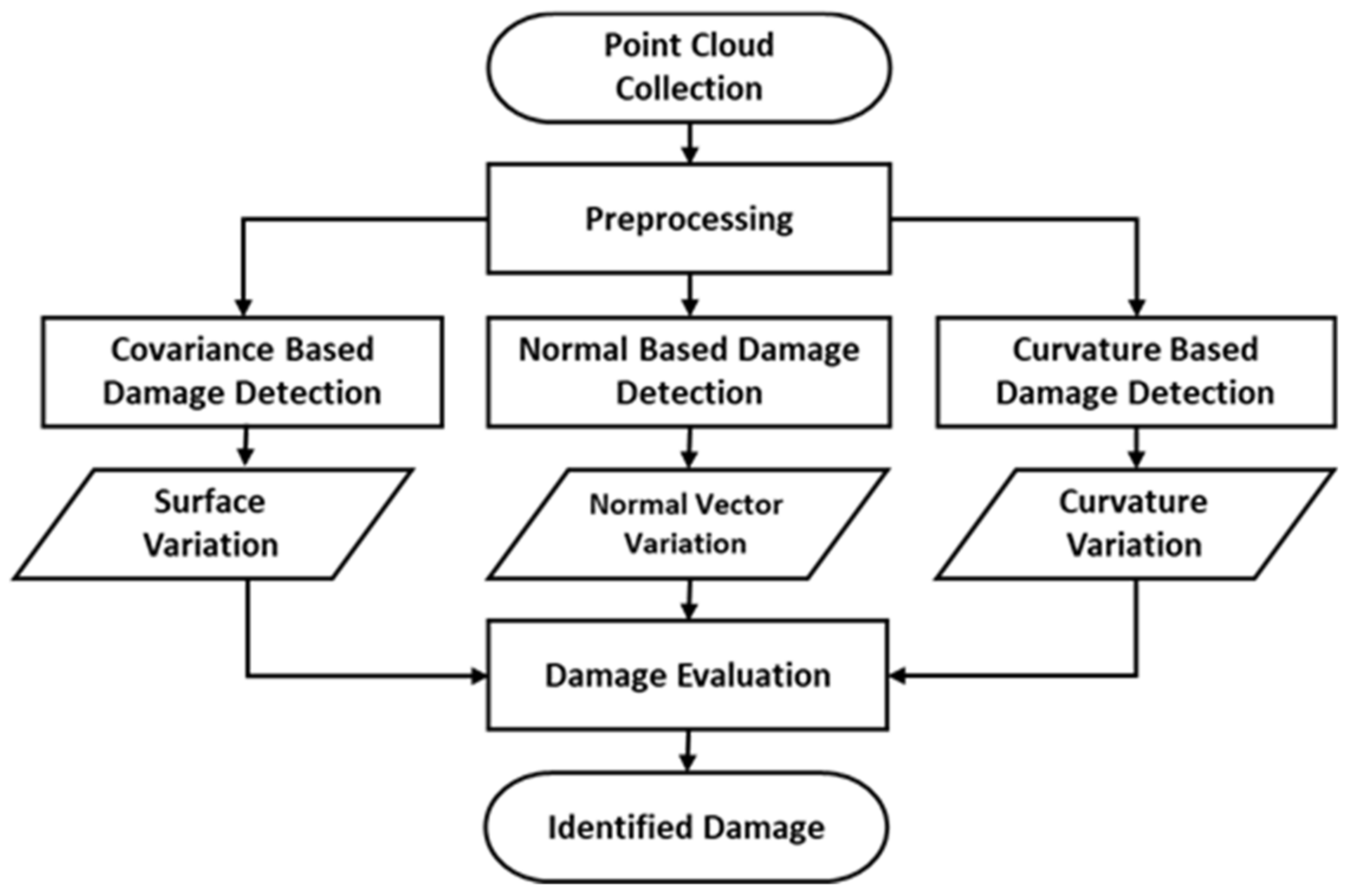
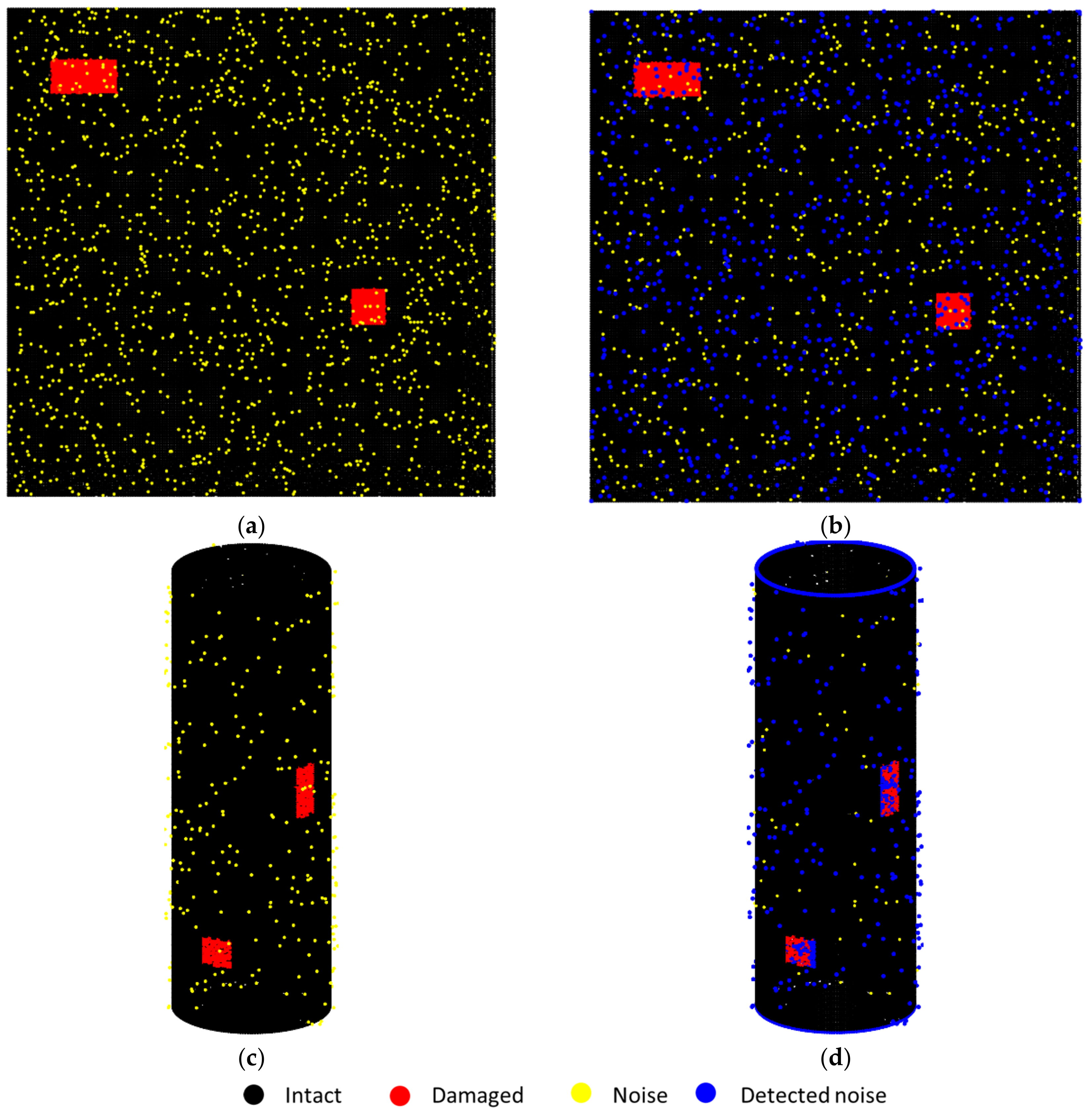
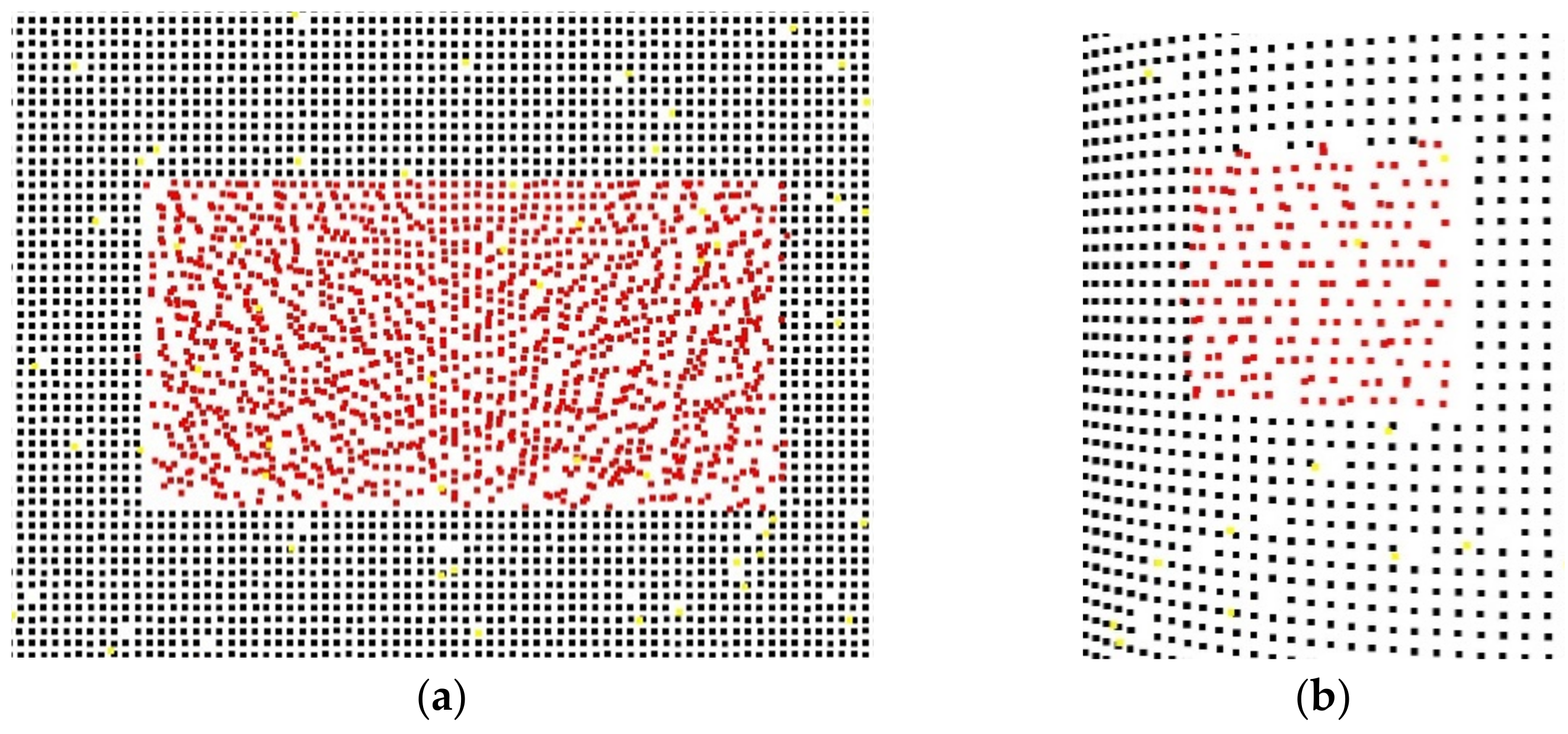
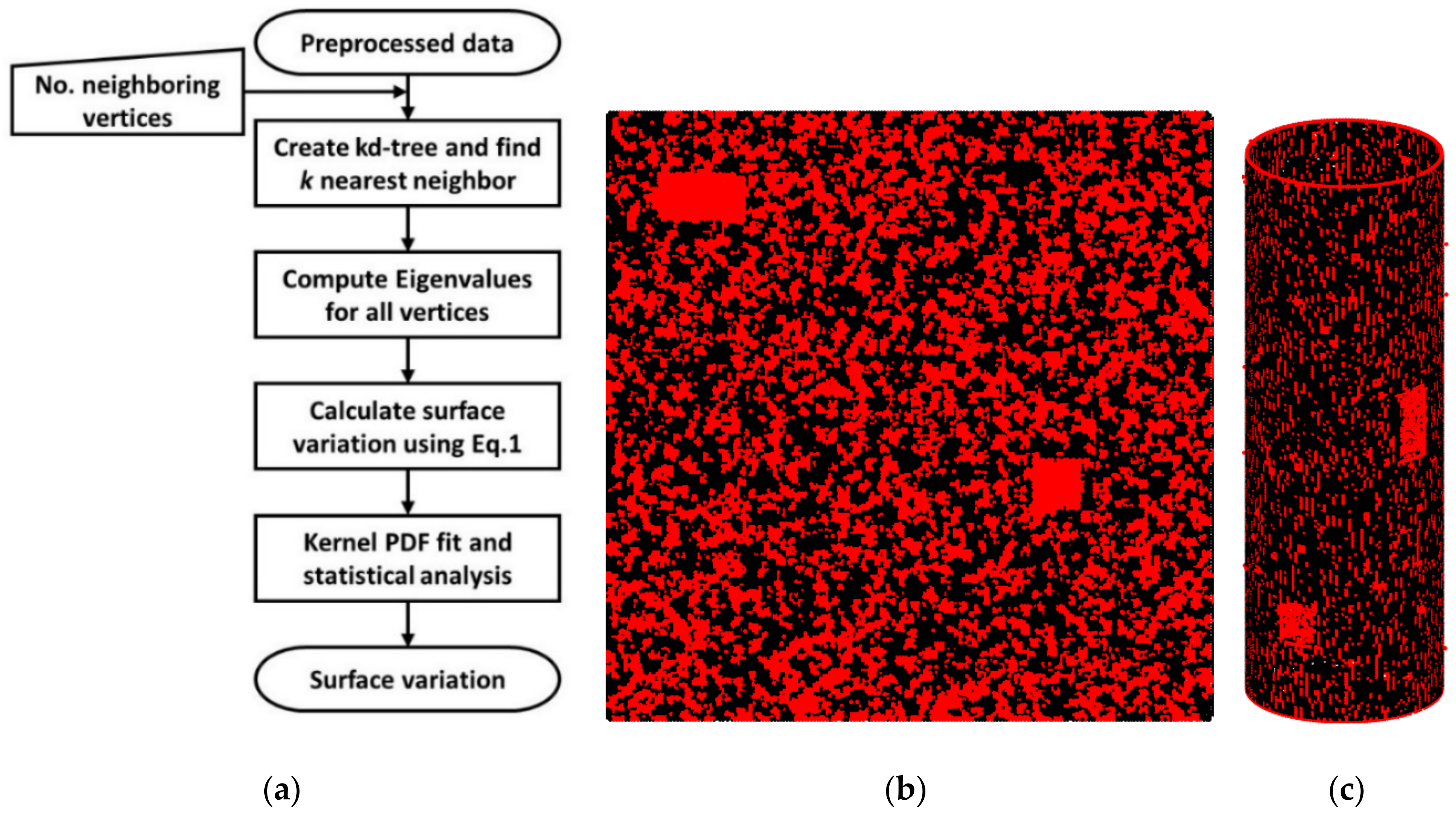
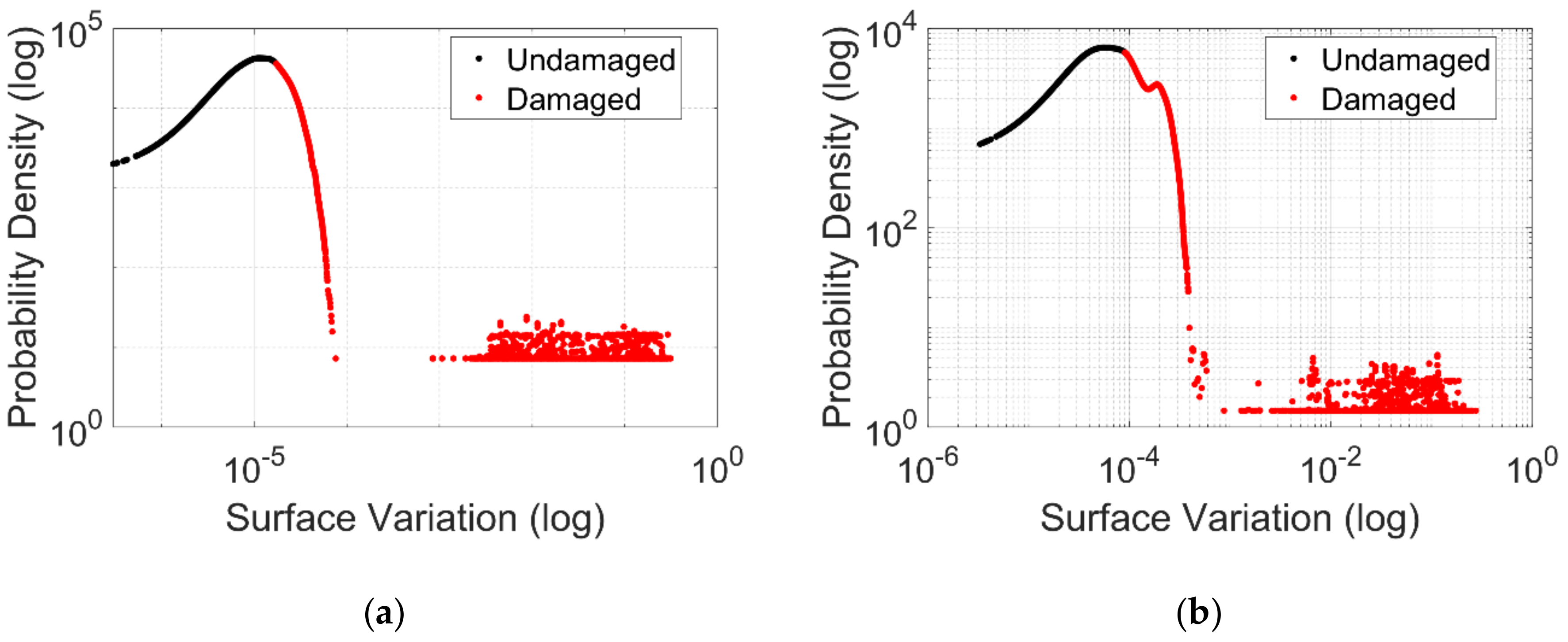
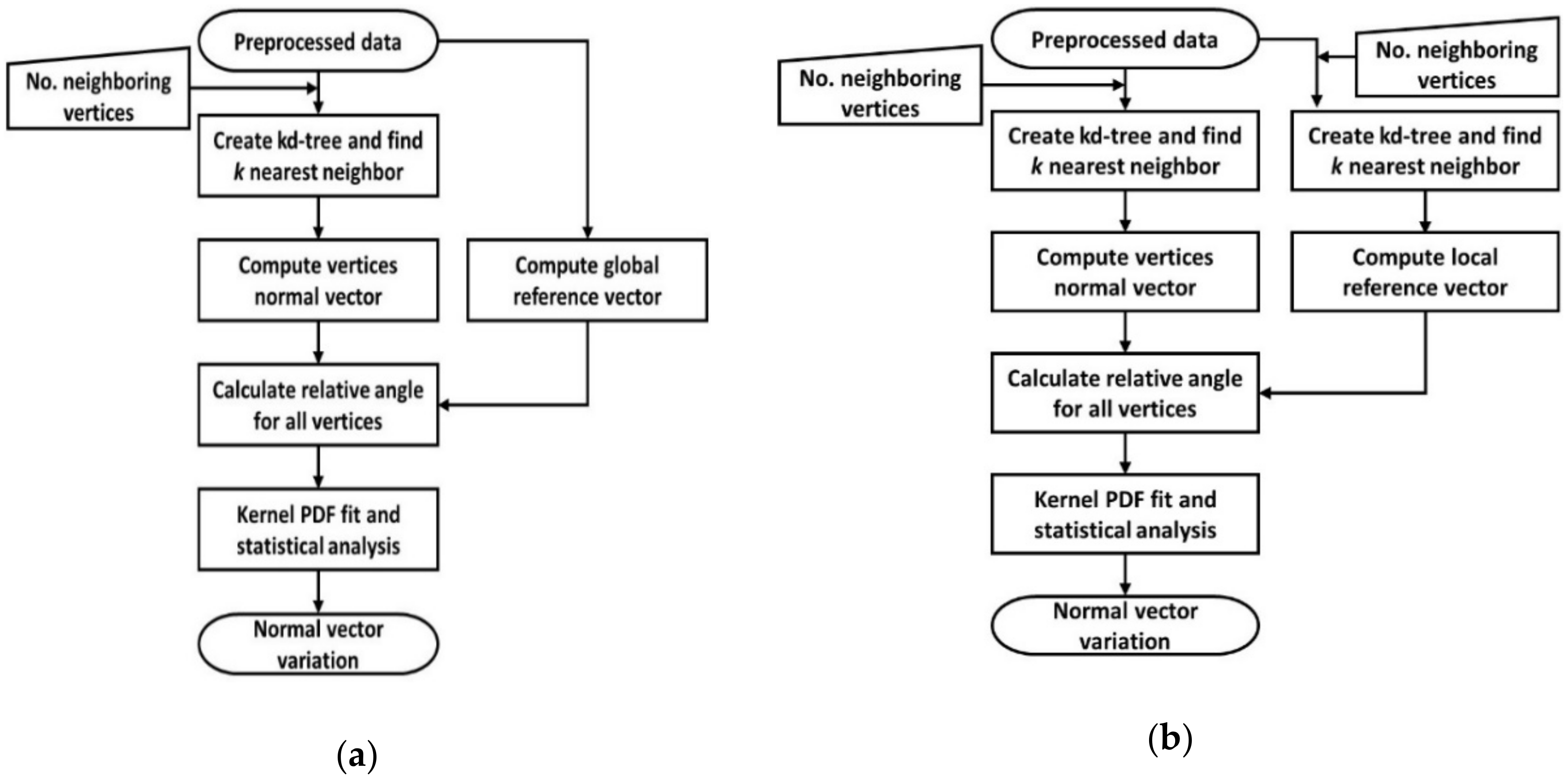
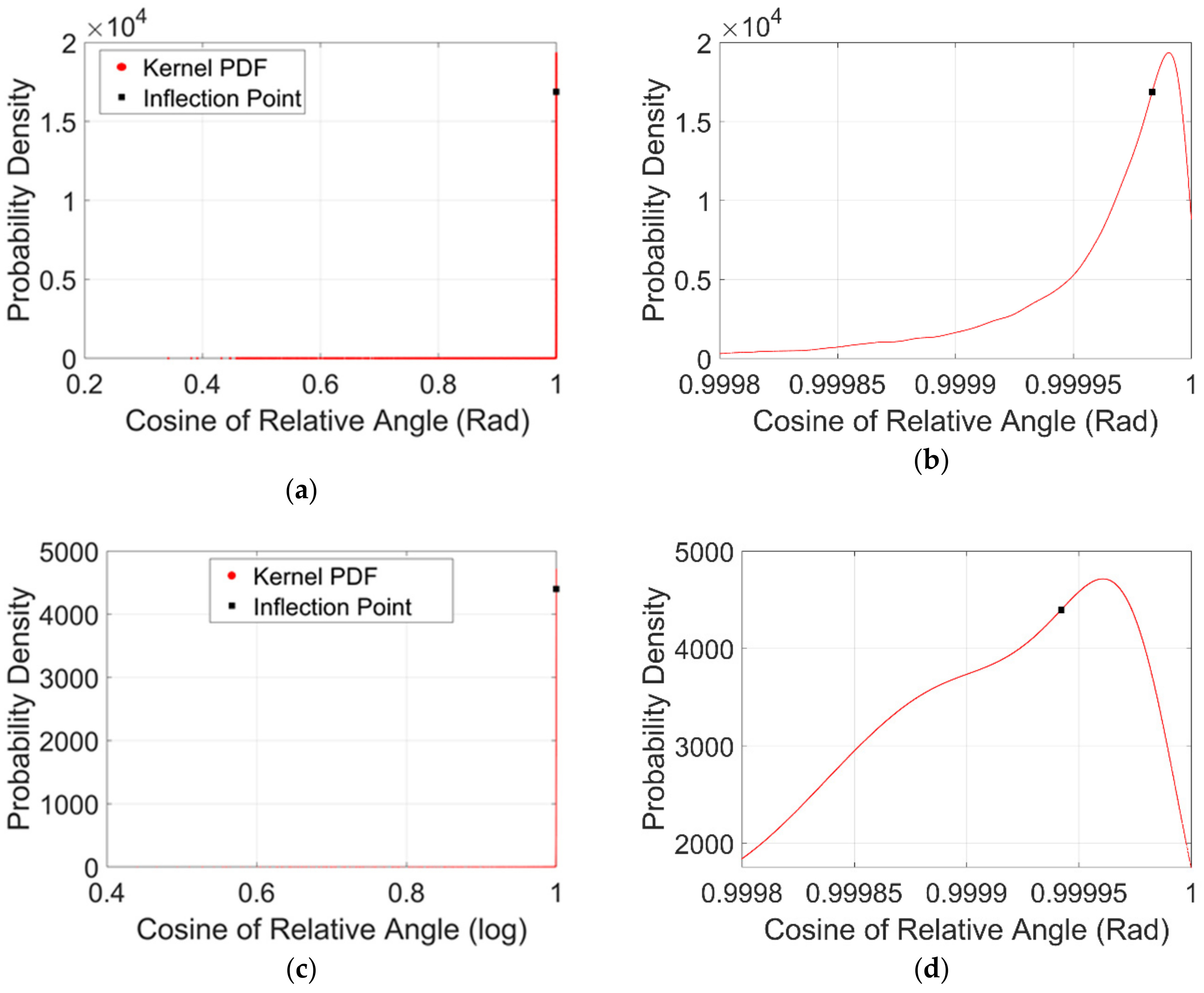
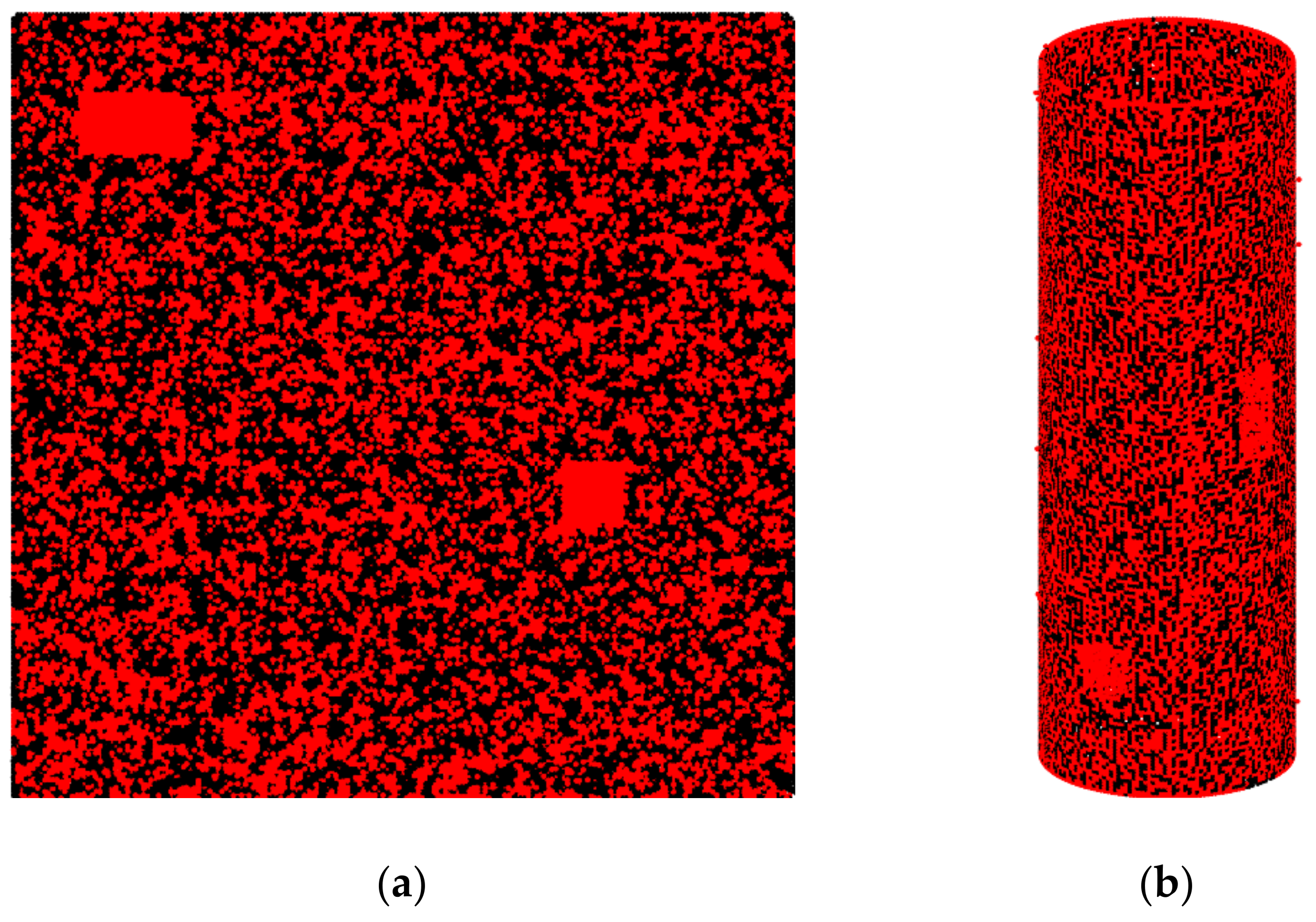
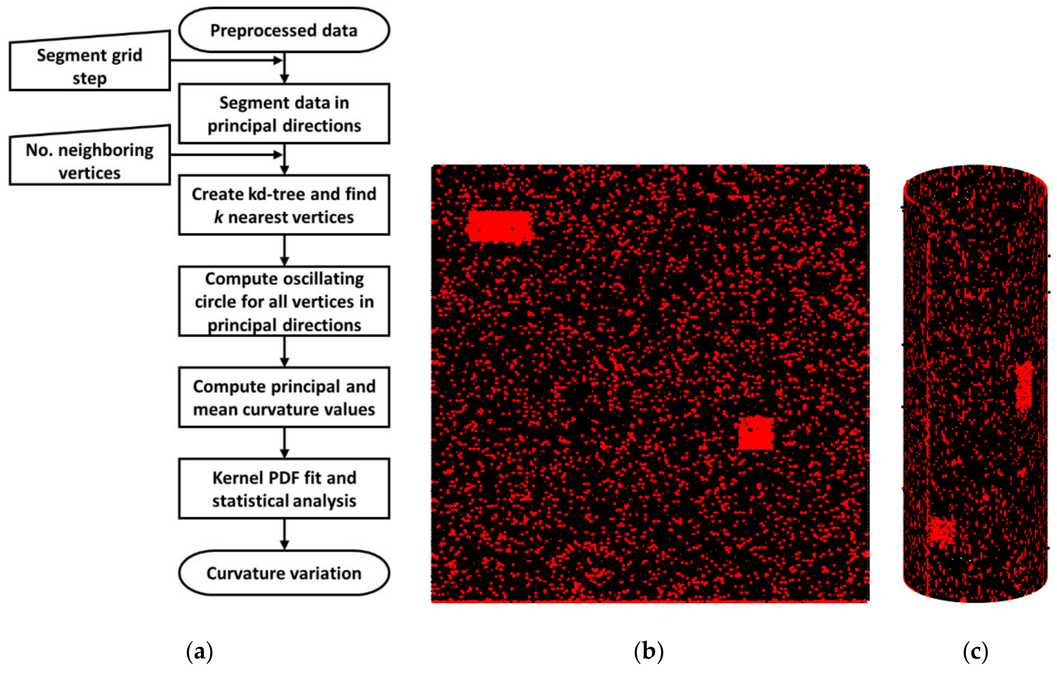
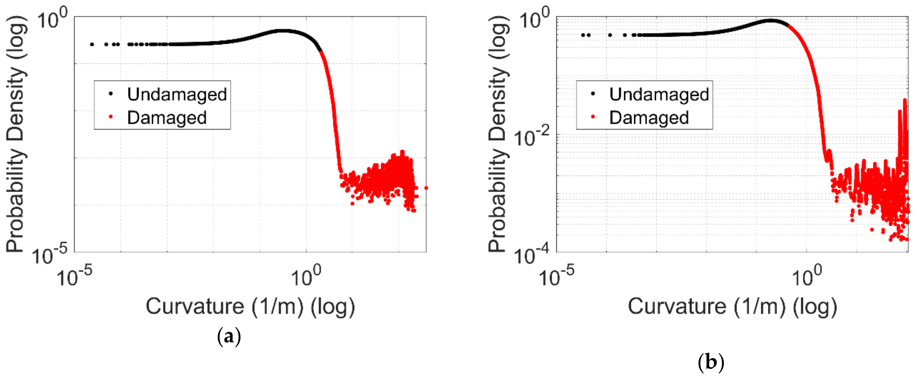
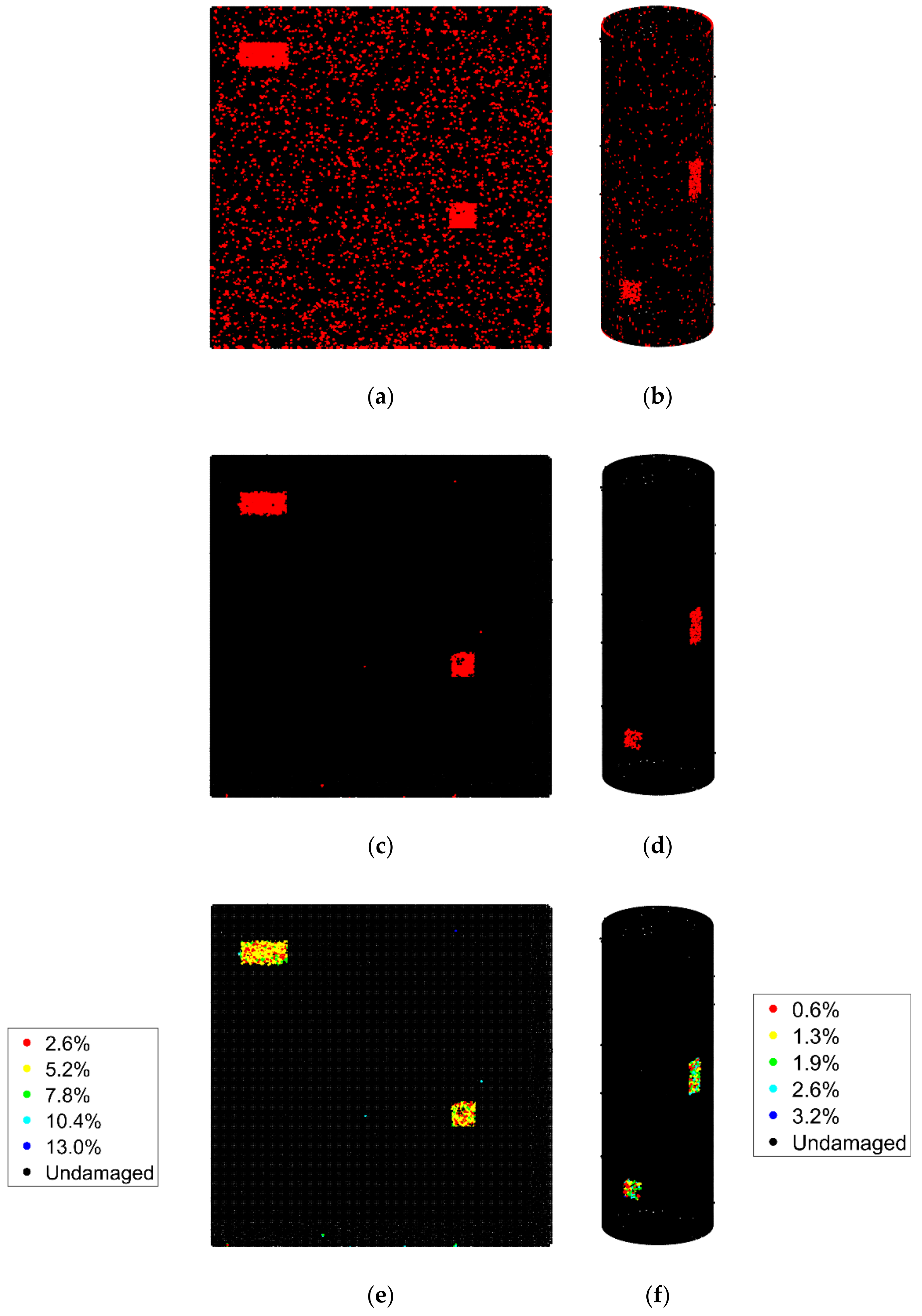
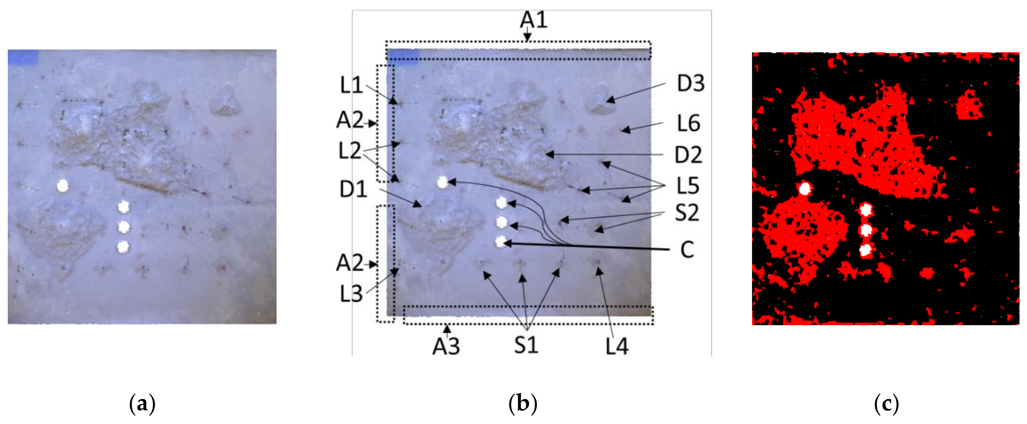
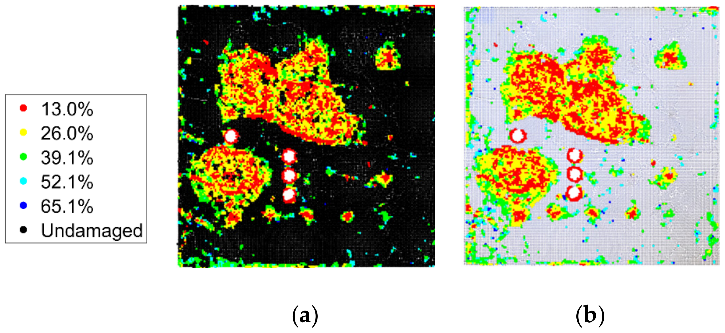
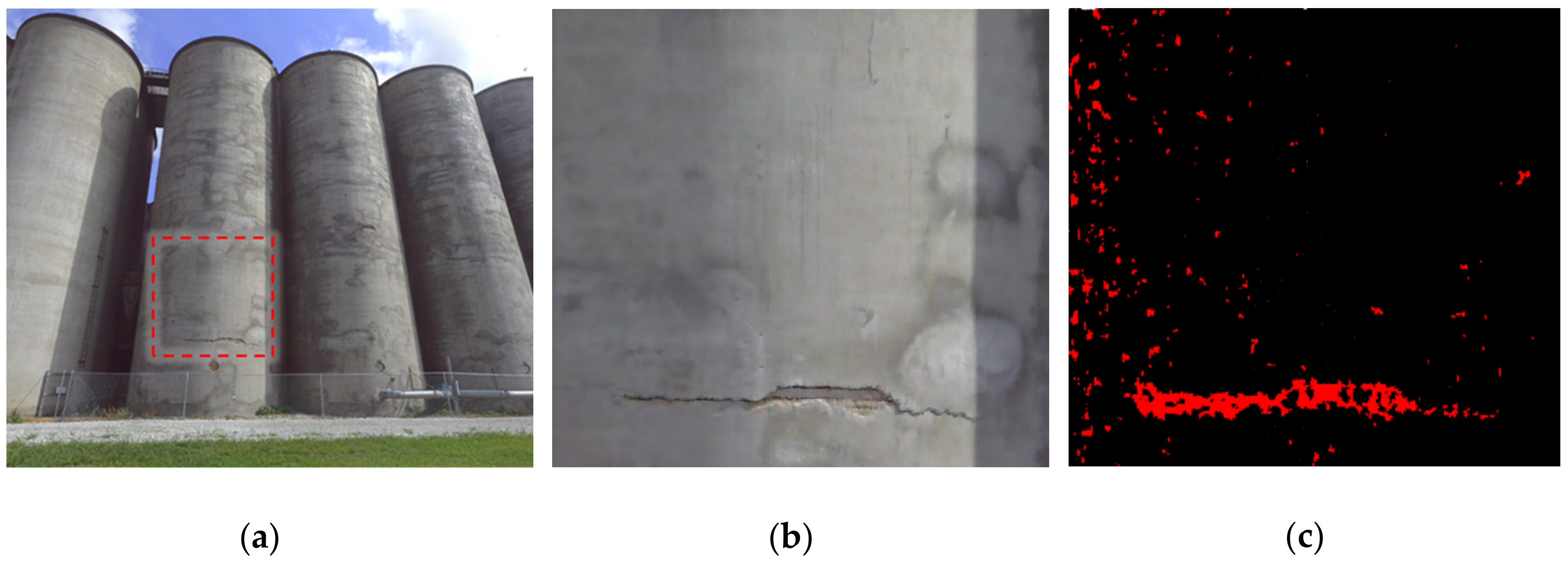
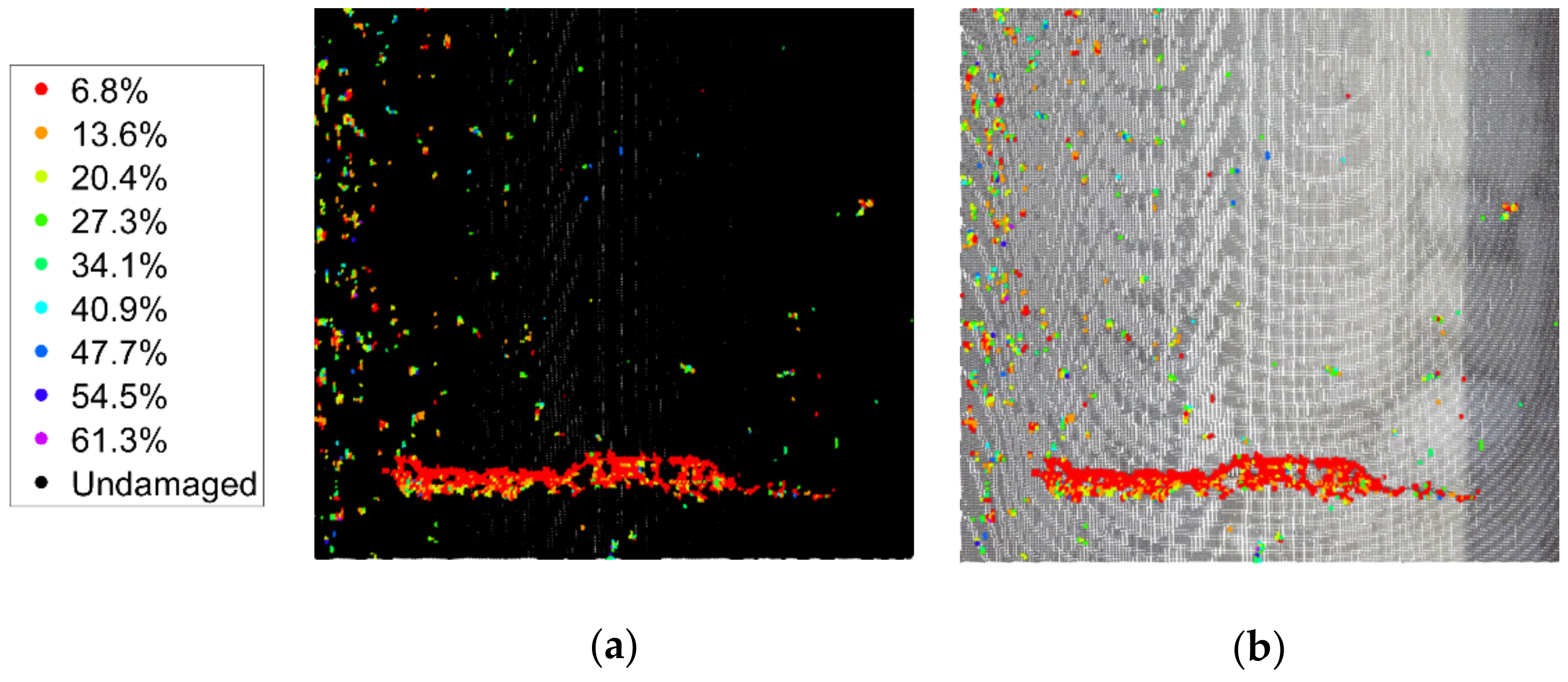
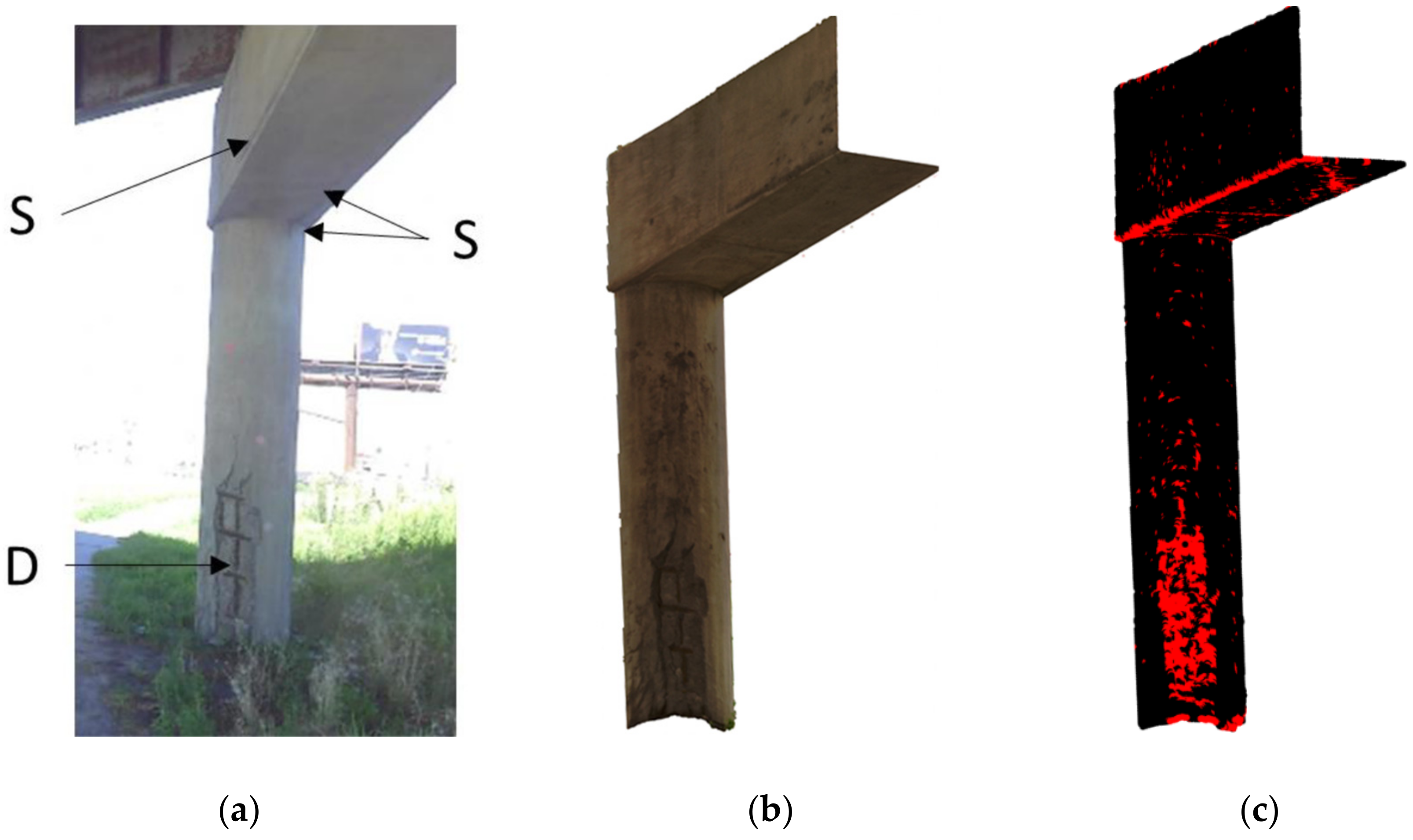
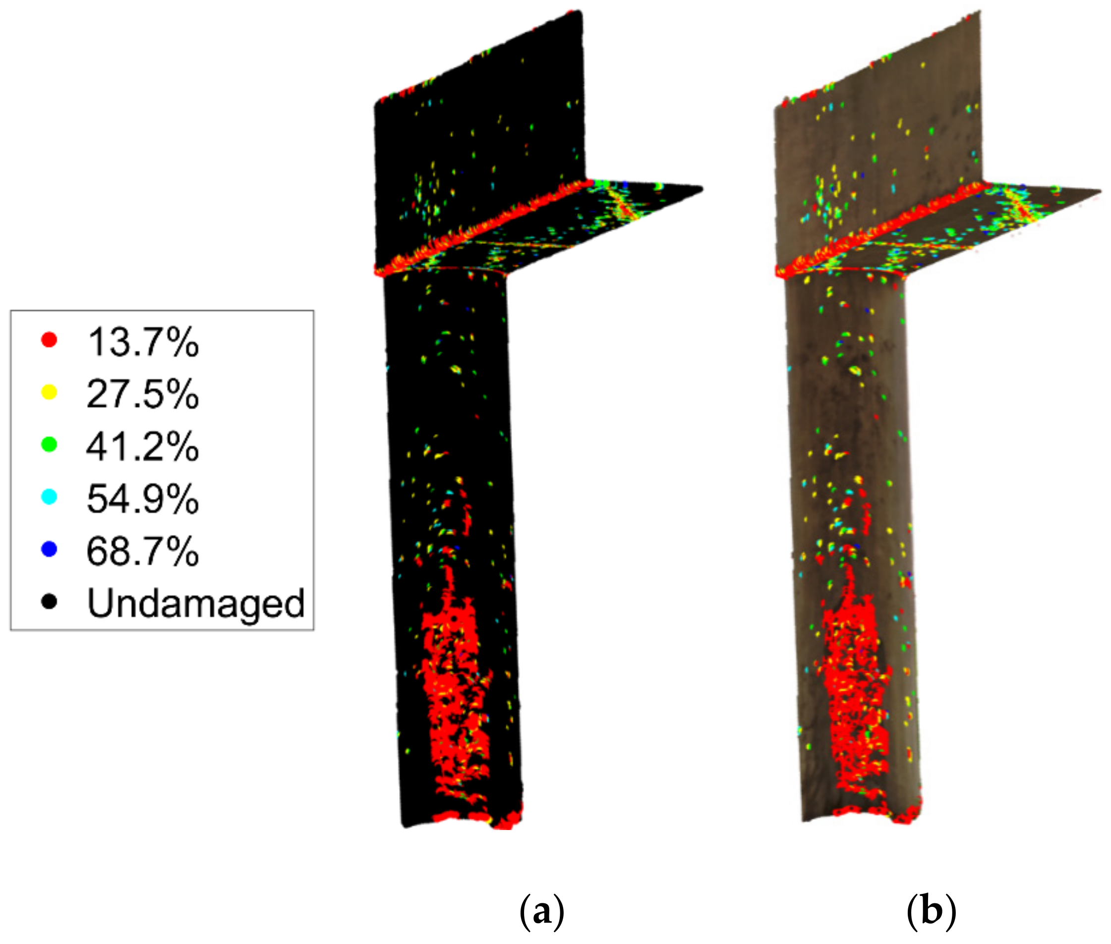
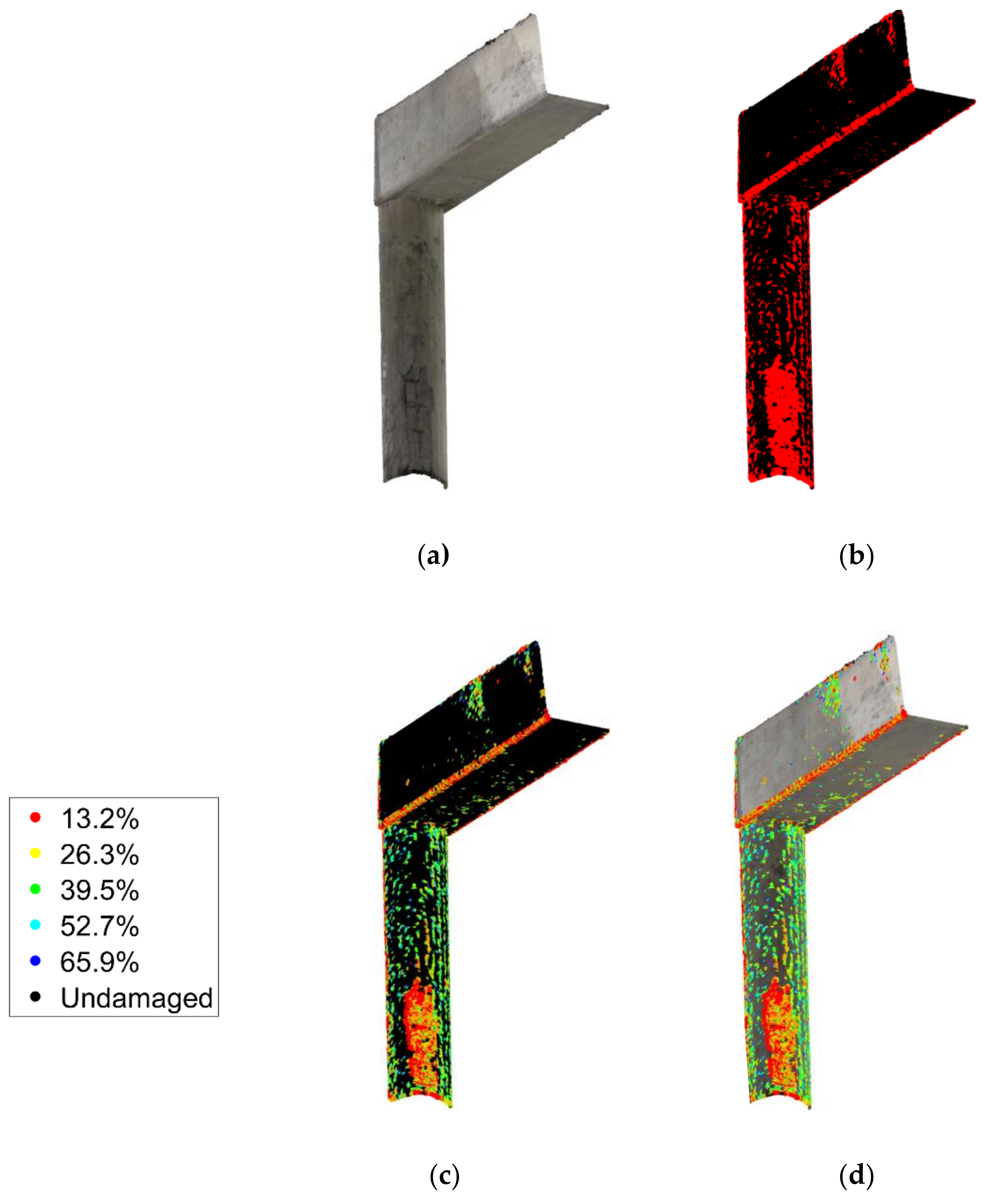
Table 1.
Performance measure for each sub-method and overall methods for the planar dataset.
| Method | Accuracy | FPR | Precision | Recall | F1 |
|---|---|---|---|---|---|
| SV | 59% | 43% | 12% | 100% | 22% |
| NVG | 55% | 47% | 11% | 100% | 21% |
| CV | 63% | 37% | 11% | 79% | 20% |
| Evaluation Step | 89% | 11% | 35% | 90% | 52% |
| Reevaluation Step | 98% | 0% | 98% | 67% | 80% |
Table 2.
Performance measure for each sub-method and overall methods for the cylindrical dataset.
| Method | Accuracy | FPR | Precision | Recall | F1 |
|---|---|---|---|---|---|
| SV | 78% | 23% | 4% | 100% | 8% |
| NVL | 41% | 59% | 2% | 100% | 3% |
| CV | 91% | 09% | 9% | 97% | 17% |
| Evaluation Step | 96% | 04% | 19% | 93% | 31% |
| Reevaluation Step | 99% | 00% | 100% | 63% | 77% |
Table 3.
Performance evaluation of the method for the slab specimen.
| Region | Measured Length (cm) | Detected Length (cm) | Percent Difference (%) |
|---|---|---|---|
| D1 | 67 | 68 | 1.4 |
| D2 | 117 | 120 | 2.5 |
| D3 | 25 | 24 | −4.0 |
© 2019 by the authors. Licensee MDPI, Basel, Switzerland. This article is an open access article distributed under the terms and conditions of the Creative Commons Attribution (CC BY) license (http://creativecommons.org/licenses/by/4.0/).
Share and Cite
MDPI and ACS Style
Mohammadi, M.E.; Wood, R.L.; Wittich, C.E. Non-Temporal Point Cloud Analysis for Surface Damage in Civil Structures. ISPRS Int. J. Geo-Inf. 2019, 8, 527. https://0-doi-org.brum.beds.ac.uk/10.3390/ijgi8120527
AMA Style
Mohammadi ME, Wood RL, Wittich CE. Non-Temporal Point Cloud Analysis for Surface Damage in Civil Structures. ISPRS International Journal of Geo-Information. 2019; 8(12):527. https://0-doi-org.brum.beds.ac.uk/10.3390/ijgi8120527
Chicago/Turabian StyleMohammadi, Mohammad Ebrahim, Richard L. Wood, and Christine E. Wittich. 2019. "Non-Temporal Point Cloud Analysis for Surface Damage in Civil Structures" ISPRS International Journal of Geo-Information 8, no. 12: 527. https://0-doi-org.brum.beds.ac.uk/10.3390/ijgi8120527
Note that from the first issue of 2016, this journal uses article numbers instead of page numbers. See further details here.