A Feasibility Study of Map-Based Dashboard for Spatiotemporal Knowledge Acquisition and Analysis

1
Chair of Cartography, Technical University of Munich, 80333 Munich, Germany
2
KRDB Research Centre for Knowledge and Data, Faculty of Computer Science, Free University of Bozen-Bolzano, 39100 Bozen-Bolzano, Italy
*
Author to whom correspondence should be addressed.
ISPRS Int. J. Geo-Inf. 2020, 9(11), 636; https://0-doi-org.brum.beds.ac.uk/10.3390/ijgi9110636
Submission received: 8 September 2020
/
Revised: 6 October 2020
/
Accepted: 22 October 2020
/
Published: 27 October 2020
(This article belongs to the Special Issue Multimedia Cartography)
Abstract
:Map-based dashboards are among the most popular tools that support the viewing and understanding of a large amount of geo-data with complex relations. In spite of many existing design examples, little is known about their impacts on users and whether they match the information demand and expectations of target users. The authors first designed a novel map-based dashboard to support their target users’ spatiotemporal knowledge acquisition and analysis, and then conducted an experiment to assess the feasibility of the proposed dashboard. The experiment consists of eye-tracking, benchmark tasks, and interviews. A total of 40 participants were recruited for the experiment. The results have verified the effectiveness and efficiency of the proposed map-based dashboard in supporting the given tasks. At the same time, the experiment has revealed a number of aspects for improvement related to the layout design, the labeling of multiple panels and the integration of visual analytical elements in map-based dashboards, as well as future user studies.
1. Introduction
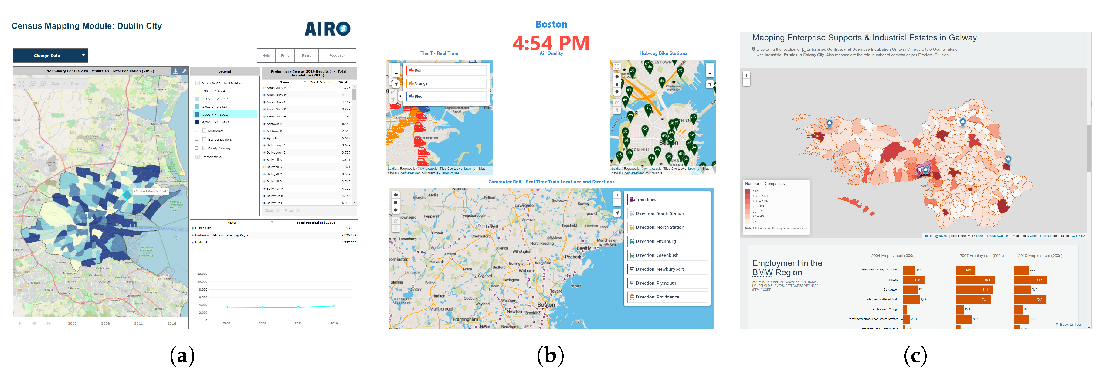
Interactive dashboard is a multimedia presentation style that concisely combines texts, images, charts, maps, videos, and gauges to allow users’ instant perception. The interactions on dashboards, such as selecting, filtering, searching, arranging, or drilling down, would additionally empower users with the flexibility to view and explore information effectively [1]. Few [2] describes dashboard as “a visual display of the most important information needed to achieve one or more objectives, consolidated and arranged on a single screen so the information can be monitored at a glance”. With the increasing amount of data available in a variety of domains, e.g., natural resources and urban infrastructures, the map-based dashboard with its dedicated components of maps and geovisualizations has become a popular tool that provides an at-a-glance overview of geospatial knowledge and supports stakeholders in making strategic decisions that lead to innovative businesses [3]. Map-based dashboard are designed to present a collection of data, and also to support the visual learning and analytical reasoning of geospatial knowledge [4]. For example, map-based dashboards are often designed to present heterogeneous georeferenced information to citizens and to encourage them to comprehend their living environments. We list several popular map-based city dashboards in Figure 1. In these city dashboards, maps are applied as the main visualization method to organize and show the information from a spatial perspective. The Dublin Dashboard (Figure 1a) is designed to display the census mapping. The spatial distribution, temporal trend, and detailed data values can be interactively retrieved via the dashboard. The Boston Dashboard (Figure 1b) shows train and bike station information on maps, giving users an overview of their locations and the distribution. In addition, the juxtaposition of the maps allow users to correlate the distributions of the trains and bike stations. The Galway Dashboard (Figure 1c) utilizes maps and charts to show various factors related to enterprise and industry. The geovisualizations in this dashboard are arranged like a waterfall on a web page so that users scroll down to check the factors one by one. In general, the map-based dashboards focus on a limited number of factors, showing the spatial and numerical distribution of the data in a self-explanatory way. The users can drill down to the data values, subsets, and a deeper understanding such as correlation and causality through simple interactions. In addition, acquiring knowledge from the dashboard has to be fast. Studies have reported that it takes less than two minutes to construct a single piece of knowledge from a dashboard [5,6,7]. It is important to note that some studies show that high-level spatiotemporal analysis is a growing need among dashboard users, such as spatial search, comparison, correlation analysis, prediction, and outlier detection [1,8]. The design of effective map-based dashboards with proper analytical functions is generally challenged by constraints such as at-a-glance display, limited viewing time, and limited user ability to understand complex geospatial data [9,10,11].
Visual analytics is a booming field for the identification and understanding of complex data patterns by combining the machine‘s computing capability and human visual perception [15]. Effective visual interface design and complex interactive visualizations have been proposed to facilitate the visual analytical procedure. For example, Robinson et al. [16] (2015) have applied visual analytics methods to identify geo-located events patterns in social media data. They have designed an interface with multiple-linked views to visualize the temporal trend, spatial locations, keywords, and detailed media texts. In a follow up study, Pezanowski et al. [17] (2017) have designed an interface of multiple linked-views with a map, a table, and a matrix to support the correlation analysis among the detected events in social media. Li et al. [18] went a step further by combining different visualizations in each view to reveal significant occurrence patterns, i.e., co-, pre-, and post-occurrence patterns for pairs of locations. They designed map multiples with a timeline to show the spatiotemporal patterns, juxtaposed bar charts and radial charts to show the (re)occurrence patterns. To satisfy the increasing demand of dashboard users on overviewing spatiotemporal distribution of regional phenomena and their relationship, we propose to integrate the visual analytics approach with dashboards and set the emphasis on the design of analytical functions following the principle of understanding at a glance. For instance, data acquisition and analysis can be better supported by dashboards after applying the high interactivity characteristics. Users may solve simple tasks (identifying, locating, and distinguishing) and complex analytical tasks (cluster identification, ranking, comparing, associating, and correlating) [1,19] by quickly viewing and interacting with a map-based dashboard. Yalçın et al. [7] (2018) have proposed a dashboard with multiple-linked views to support novice users to identify tabular data patterns. They used maps and basic charts (bar chart, line chart, and pie chart) in each view to present a perspective of a dataset. Nazemi et al. [19] (2019) proposed a dashboard with the juxtaposition of visualizations such as a map, a chord diagram, small multiples, and a bar chart to allow users to perform analysis and comparison tasks.
Whether dashboards are useful and effective depends highly on user-centered evaluation [20]. User studies are commonly used to evaluate various types of cartographic visualizations. Numerous studies have focused on investigating the influence of specific design elements on interactive maps. Evaluating the user experience and usability of the geovisualizations in high-level spatial insights construction should be further studied [21,22,23]. Andrienko et al. [24] have proposed two types of analysis tasks, i.e., identification and comparison, to evaluate analytical geovisualizations. These two types of tasks differ in cognitive operations. The identification tasks focus on finding the characteristics of objects or locations. The comparison tasks require one to compare or summarize characteristics in different times or places. Yalçın et al. [7] have grouped the insights constructed by users into five categories: fact, min/max, correlation, distribution, and comparison. Bogucka et al. [25] proposed benchmark tasks that differ in query types, search output, and cognitive operations. In our work for the evaluation of the designed map-based dashboards, we propose three identification tasks and three reasoning tasks, each differing in search output, query type, dashboard interaction, and data uncertainty.
Popular methods for the evaluation of map-based dashboards include survey, interview, think-aloud, and eye-tracking [26]. Robinson et al. [16] have evaluated their map-based interface with a task-solving session and a survey on 25 domain experts. These two tasks were open-ended tasks, requiring the users to understand spatiotemporal patterns. In their survey of usability and utility, they applied the System Usability Scale method [27]. In a further study, Pezanowski et al. [17] have conducted an online usability and utility survey with 23 completed responses out of 327 participants. Many evaluations are done by interviewing the experts [18,28,29,30,31]. The expert interview gives self-reported outcomes, but the outcomes could be biased. McKenna et al. [32] and Yalçın et al. [7] conducted an evaluation on their dashboards by the think-aloud method during free exploration and a post-survey. The think-aloud session can reflect the usability in a natural usage scenario. Many studies use the eye-tracking method to externalize the knowledge construction procedure of users in viewing geovisualizations. In such studies, the authors collect and analyze eye movements when users are performing the predefined tasks. Hegarty et al. [33] found that users are more likely to be attracted by visually complex visualizations than simple ones. Opach et al. [34] have used the eye-tracking method to study the viewing strategy of users in obtaining insight on multi-component animated maps. They analyzed the order of response accuracy, fixation durations, dwells and transitions of the area of interests (AOIs). Bogucka et al. [25] accessed the feasibility of a space-time cube by analyzing the tasks’ complete rate, duration, and search strategy from the eye movement data. Popelka et al. [35] have evaluated analytical maps by analyzing participants’ attention, fixation sequence, and comparing the viewing points between correct and wrong answers. They formed a set of suggestions for the map-based interactive analytical application design.
In this study, we evaluated the effectiveness and efficiency of our proposed map-based dashboard by means of eye-tracking and interviews. The evaluated map-based dashboard is composed of multiple linked-views, and aims at supporting users in acquiring and analyzing geo-knowledge, such as spatial distribution, clusters, correlation, and temporal trend, at a glance. The dashboard is implemented as a web-based prototype so that users can interact with it during the experiment. Our experiment consisted of two major components. First, we designed six tasks and collect the eye movement data when the participants were performing the tasks. Next, we interviewed the participants about their attitudes towards the dashboard. We then analyzed the eye-tracking data and interview results using a variety methods to reflect the effectiveness and efficiency of the dashboard. The remainder of this paper is structured as follows: Section 2 introduces the design of the map-based dashboard. Section 3 describes the design of the experiment. In Section 4, we analyze the results of the experiment. Section 5 discusses the performance of the dashboard and the limitation of our experiment. In Section 6, we provide our conclusions from this study and offer outlooks for the future.
2. Design of the Dashboard
This section introduces the background for designing and implementing the dashboard, the test data, and the visual user interface of the proposed map-based dashboard.
2.1. Background
In a fast-developing society, stakeholders in many domains are updated with rapidly and constantly changing information about their surrounding economic environment. McKenna et al. [36] have studied the information needs of different stakeholders in an enterprise. The analysts need the most detailed information to understand how each factor changes at each location and time. The managers and directors need more general information, such as data distributions and trends. The chief executive officers (CEOs) need the most general information, and they care more about the future trend rather than historical events. Previous studies have suggested that dashboards serve as an effective tool for stakeholders in their decision-making procedure [1,37]. According to the information needs of stakeholders, dashboards are categorized into three main types according to their roles: operational, analytic, and strategic [2]. The operational dashboards aim to monitor the situation with a high temporal resolution and use dynamic visualizations to show the changes in detail. The analytical dashboards present patterns at a higher abstract level, and provide interactions for users to explore further information. The strategic dashboards provide an overview of the most general information and require fewer updates and interactions.
A map-based dashboard was designed in this study for stakeholders like leaders of small and medium-sized enterprises (SMEs) and citizens. These stakeholders need the overview information as well as certain analytical functions to understand and analyze the factors of the economic environment to make their decisions. They want to answer typical questions such as how high the population density in a city is, how much the average income of the citizens is, what is the trend of the economic-related factors in recent years, and how the economic development and transportation infrastructure correlate. Thus, we have designed our dashboard as an analytical map-based dashboard that not only shows the overview of the spatiotemporal patterns of multiple economic factors, but also supports users to fulfill their analytical tasks.
2.2. Test Data
Our test datasets are socioeconomic data at the municipality level provided by Yangtze River Delta Science Data Center (http://nnu.geodata.cn:8008/). The datasets originated from the census data. The datasets cover various topics, including gross domestic product (GDP), public investment, industrial output, population, and employment. In this study, we have selected four representative categories of socioeconomic environment, including enterprise, GDP, population, logistic, and have further identified 22 related factors in these four categories. The temporal coverage is from 2013 to 2015, where the data is available in most municipalities. Table A1 in the Appendix A shows the categories and factors used in this study.
We have chosen Province Jiangsu, China as the study area. Jiangsu is located in the east of China, at the lower reaches of the Yangtze River, which covers 107,200 km and 98 municipalities. The sizes of the municipalities vary from 54 km to 3059 km. With over 80 million people, Jiangsu is among the most densely populated and economically fastest developed regions in China. In recent years, the industry structure is undergoing rapid transformations in Jiangsu. Therefore, mastering the local economic conditions is very valuable for the stakeholders.
2.3. User Interface
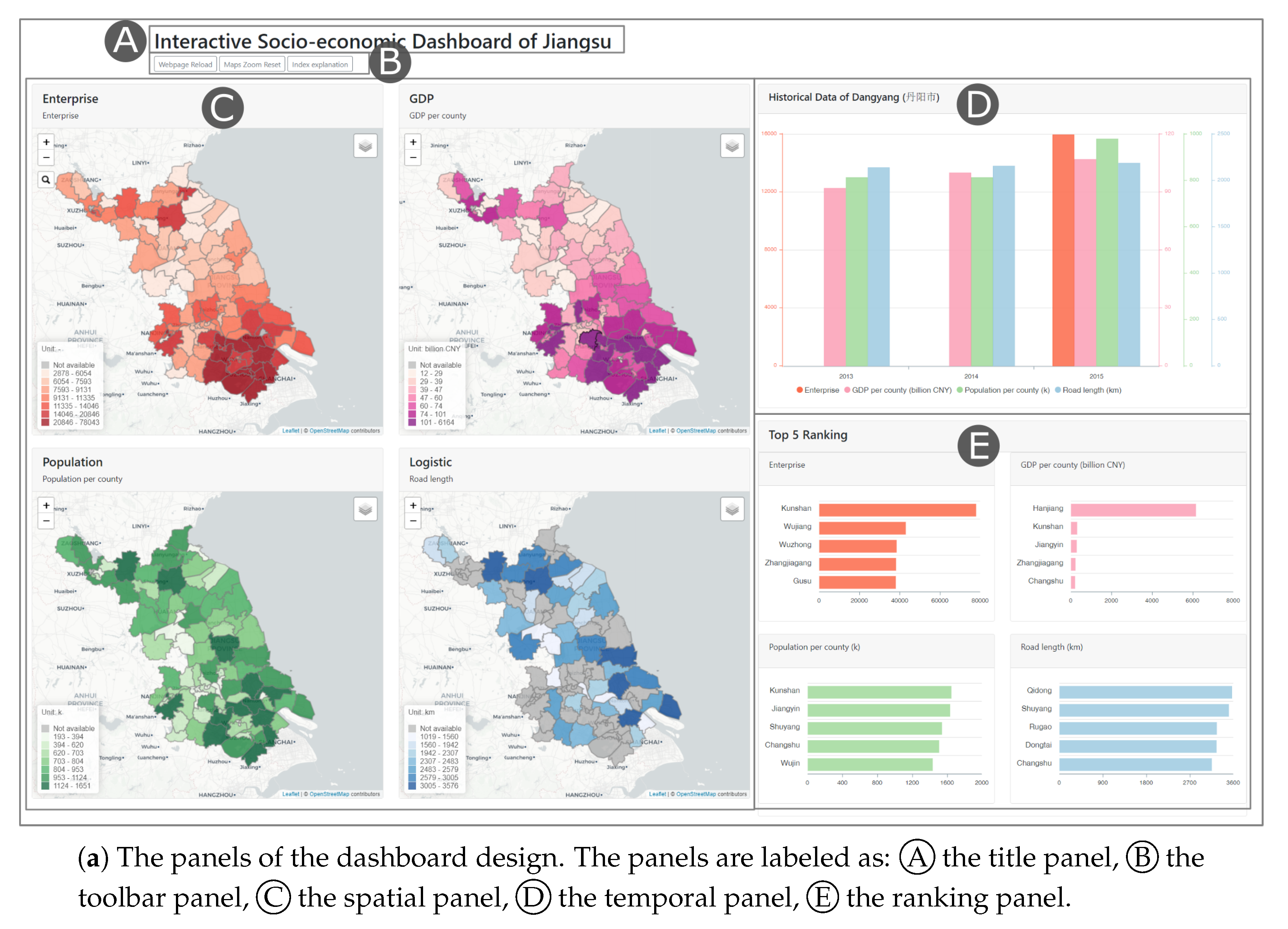
We aim to show the users the overview of the spatiotemporal patterns of various economic factors, reveal their correlations, and allow users to compare the patterns at different levels of detail. The interface of our dashboard consists of five panels, (A) the title panel, (B) the toolbar panel, (C) the spatial panel, (D) the temporal panel, and (E) the ranking panel.
Figure 2a shows the interface and its components. The title panel shows the topic of the dashboard. The toolbar panel allows users to reset maps, reset selections, and read explanations to various factors. The spatial panel presents the spatial distribution of multiple factors on maps. Each map shows a socioeconomic category, i.e., enterprise, GDP, population, and logistics. There are several layers within each map, and each layer shows one factor. The temporal panel shows the temporal trend of the data distribution along time. When a county is selected, its historical data is displayed as a bar chart in the temporal panel. The ranking panel presents the top five municipalities from the four economic categories respectively. The color scheme of these panels is kept consistent. Each category of factors is represented with a single-hue color scheme, where category enterprise is represented in red, GDP in purple, population in green, and logistic in blue.
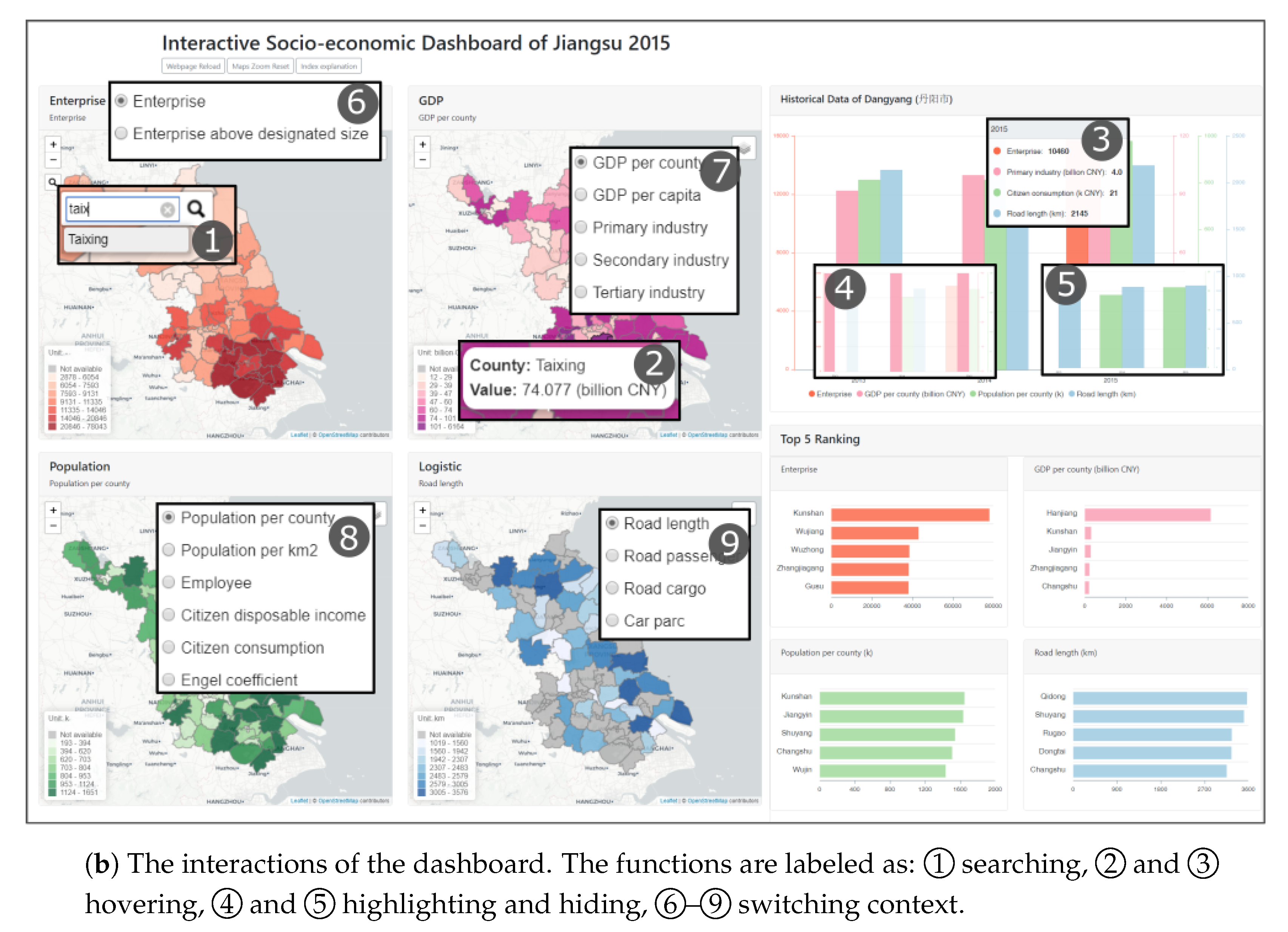
Moreover, the interactions are shown in Figure 2b. The spatial, temporal, and ranking panels are linked, and serve together as an at-a-glance representation of the economic condition of the study area. The search function allows users to locate any county in the area. When a county is searched, the maps are zoomed in to this county and the temporal data of the searched county are shown. The factors can be selected by the switching function. Whenever a county or a factor is selected on one panel, this selection is applied to other panels. The four maps are sychronized in zoom level and central point. When users move one map, the others follow. Last but not least, users can reset the maps, reset the whole dashboard, and read the available factors and the their detailed information (see Table A1) by clicking the buttons on the toolbar.
This dashboard design allows users to retrieve detailed information on demand. For example, users can retrieve the value of a factor of a certain municipality in a certain year. Furthermore, the dashboard supports users in obtaining high-level knowledge. For instance, users can learn the temporal trend of a factor, compare the spatiotemporal distributions of factors in different municipalities, compare the patterns of several factors of one specific municipality, or visually find correlation among factors. The dashboard interface was developed in JavaScript. The maps and charts were developed based on open source libraries such as Leaflet (https://leafletjs.com/) and ApexCharts.js (https://apexcharts.com/). We used Bootstrap (https://getbootstrap.com/) to arrange the layout of the dashboard. The interface can be browsed in various web browsers, such as Google Chrome, or Firefox.
3. Design of the Evaluation Experiment
This study aims to access the feasibility of the map-based dashboard for knowledge acquisition, especially with regard to spatiotemporal patterns and correlations in socioeconomic data. We have designed a qualitative study to collect and analyze the performance of the dashboard. More specifically, we have evaluated the effectiveness and efficiency of the dashboard by analyzing participants’ gaze behavior and studying their attitudes towards the dashboard. To achieve this, we set up several benchmark tasks at several difficulty levels and designed an eye-tracking experiment to collect the participants’ visual attention. Then we conducted an interview to collect feedback. In this section, we describe the design of these evaluation methods in detail.
3.1. Participants
We recruited 40 participants with the means of short introductions in classrooms, posters on the campus, and online advertisements. One of the participants dropped out of the experiment due to near-sightedness. The remaining 39 participants had normal or corrected-normal eyesight and completed the experiment. After the experiment, we found that the eye-tracking ratios of seven participants were less than 70%, and could not be considered. Thus, the analysis was based on the recoded eye movement data from the remaining 32 participants. Among the 32 participants, there were 17 females and 15 males. Their average age was 25.9, with a standard deviation of 2.36. The participants had diverse educational backgrounds: one participant had high school or equivalent degree, 17 participants had bachelors’ degree, and 14 participants had masters’ degree. They had various interactive dashboard usage experience. Twelve participants had used dashboards more than five times, five participants had used less than five times, eight participants had heard about it but not used, seven participants had never heard about it. In addition, none of the participants had ever lived in the study area. To clarify: in this paper the participants are the volunteers who took part in our experiment, the users refer to our target users of the designed dashboard.
3.2. Apparatus
We used a Gazepoint GP3 eye tracker, equipped with the software Gazepoint Analysis to collect eye movement data. The eye tracker has a 0.5–1 degree of visual angle accuracy and 60 Hz update rate. As Figure 3 shows, the eye tracker was placed under a monitor. We used two 2560 × 1440 resolution DELL monitors, one of which was for the participants to explore the dashboard, another for the controller of the experiment. The dashboard was running on a local server with Google Chrome as the browser. The participants were provided with a keyboard and a mouse to interact with the dashboard. The experiment environment was set up in the eye-tracking lab at the Technical University of Munich. The experiment lab was in a stable, quiet condition, and with scattering light during the experiment.
3.3. Benchmark Tasks
Considering the tasks in [7,24], Zuo et al. proposed four benchmark tasks in dashboard usability testing in [38], which differ with regard to cognitive operations. However, the tasks were open-ended and caused great variations in participants’ answers. In this study, we have proposed six close-ended benchmark tasks in different cognitive operations and dashboard interactions. These tasks belong to two types: (1) identify specific value(s) from the dashboard, and (2) compare or summarize high-level knowledge based on the facts found via the dashboard. For each type we proposed three specific tasks with increasing difficulty. The tasks were presented as statements that should be judged by the participants as being correct, wrong, or unknown based on their interactions with the dashboard. Table 1 describes the six statements and their associated answers.
The execution of these proposed tasks involves different search areas, periods, attributes, querying types, cognitive operations, dashboard interactions, and data availabilities. Table 2 outlines the complexity of each task in the aforementioned aspects. T1, T2, and T3 require participants to locate a value (or more) from the dashboard and make basic comparisons. The cognitive operation difficulty increases from T1 to T6. T1 requires participants to only find a value of an area. T2 requires participants to compare the values in an area. The cognitive complexity of T3 is higher than T1 and T2, because participants need to compare the values of multiple areas. T4, T5, and T6 require participants to summarize the patterns from multiple areas. T5 is slightly more complex than T4, because more search attributes and more dashboard interactions are involved. T6 is the most difficult task, because it requires participants to deduce the results from incomplete data, and the participants need to understand the economic concept “industrialized level”.
3.4. Experiment Tool
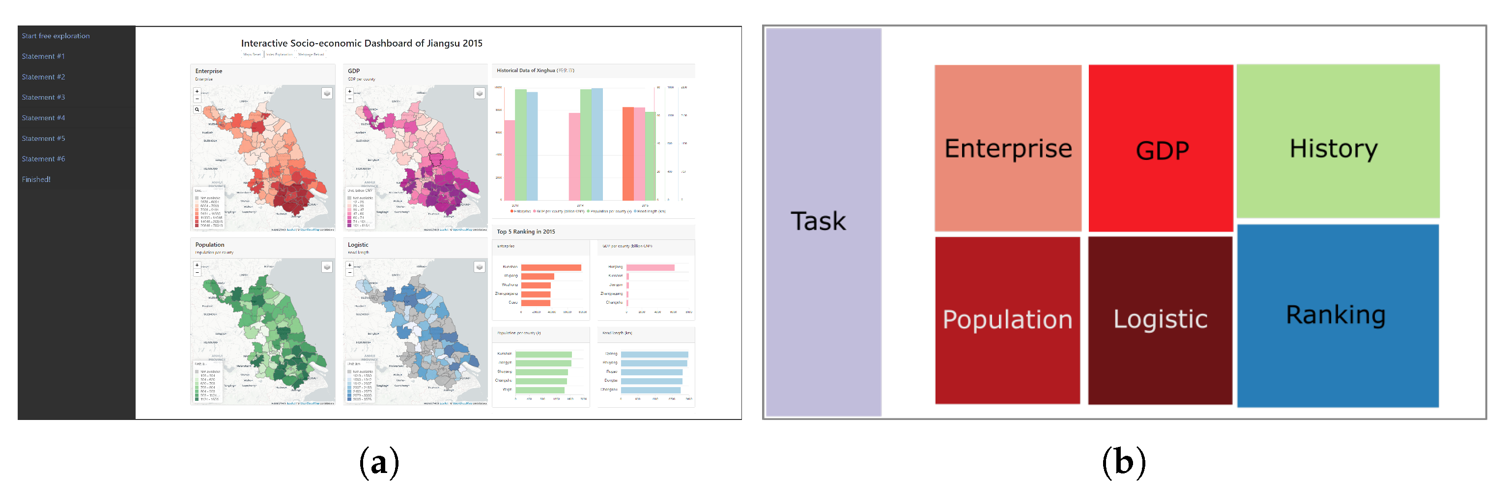
To guide participants through the hands-on part of the experiment, we developed an interactive experiment tool on the dashboard interface. As shown in Figure 4, the tool is in the left side of the dashboard with a dark background color to differentiate with the data visualization panels. It consists of eight items, including the first item of “Start free exploration”, the six items of Statement 1–6, and the last item of “Finished!”. When an item is clicked, the item expands with a concrete instruction of the step. When the item Start free exploration is clicked, it shows the instruction of “Please start tasks in 3:00 minutes!”. The number is a real-time countdown clock to remind participants of the remaining time during the free exploration. Note that the six tasks were shown in a random order for each participant in the Statement items. Thus the influence of the order for the response time of tasks was be minimized. The item “Finished!” confirmed the completeness of tasks and informed the participants that they were free to move their bodies. The participants were asked to click the items following the order from top to bottom. Only one item could be clicked at one time. After clicking a new item, the dashboard on the right side is reset.
3.5. Procedure
The experiments were conducted from 26th November 2019 to 21st December 2019, in the Eye-tracking lab at the Technical University of Munich. The experiment was conducted in consecutive order, with one participant following the other. The participants were allowed to terminate the experiment at any time. The experiment consisted of six steps: pre-experiment, introduction, calibration, free-exploration, task-solving, and interview. In addition, all the steps were carried immediately after the other. In this section, we introduce each step in detail.
Pre-experiment. Before the experiment, each participant had several minutes to relax, because we found that many participants were too nervous or excited to start the experiment directly. When the experiment started, we first informed the participants about the data protection policy, the approximate duration, the experiment steps, and the data collection. If the participant agreed, we would proceed with the experiment. The participants were then asked to fill out a form with their personal information, including gender, age, education level, and dashboard usage experience.
Introduction. We conducted a standard introduction for the participants. The introduction included a short description of the factors and operation tutorial of the dashboard, namely data categories and factors, panels of the dashboard, and the experiment tool. The participants were allowed to ask usage-related or general questions in this step. Additional information that might have influenced the results of the experiment was not given.
Calibration. First, we asked the participants to find a comfortable position while keeping their eyes within the detection range of the eye-tracker. We informed the participants that they needed to hold the position during the calibration, free exploration, and the task-solving steps. We then repeatedly calibrated the eye tracker until it met the experimental requirement.
Free-exploration. During this step, the eye movements of the participants were tracked. Every participant was asked to explore the dashboard freely for three minutes. All the participants were allowed to view or interact with the dashboard freely. They began this step by clicking the Start free exploration item on the experiment tool. They could check the time with the countdown clock on the experiment tool, or the experiment controller would remind the participants when the time was up.
Task-solving. The task-solving step was also performed while the eye movements was being tracked. The participants solved the tasks following the order of Statement showing on the experiment tool. After clicking and reading the task item, they could interact with the dashboard and check the answers as correct, wrong, or unknown on a prepared sheet. After finishing a task, they were only allowed to proceed to the next task and could not return to or change any previous answers. The tasks did not have a time limit for completion.
Interview. In the last step, we interviewed each participant with four questions. First, we asked the participants to rate their confidence levels of the answers in the range of 1 (not confident at all)–10 (very confident). Second, we asked them to rate the difficulty level of using the dashboard between 1 (very hard)–10 (very easy). Third, we asked them to list the design elements that helped them during the completion of the tasks. Lastly, we asked them to list the design items or elements that were not easy to understand or interact with. During the discussion, the participants were also asked to describe more whenever necessary. The answers of the participants were recorded as written protocols.
3.6. Methods of Analysis
We analyzed the acquired eye-tracking data and the interview results to assess the performance of the designed map-based dashboard. We focused on analyzing five themes: the attraction of the panels, the effectiveness of the dashboard, the efficiency of the dashboard, the task-solving strategy of the participants, and their attitude towards the dashboard.
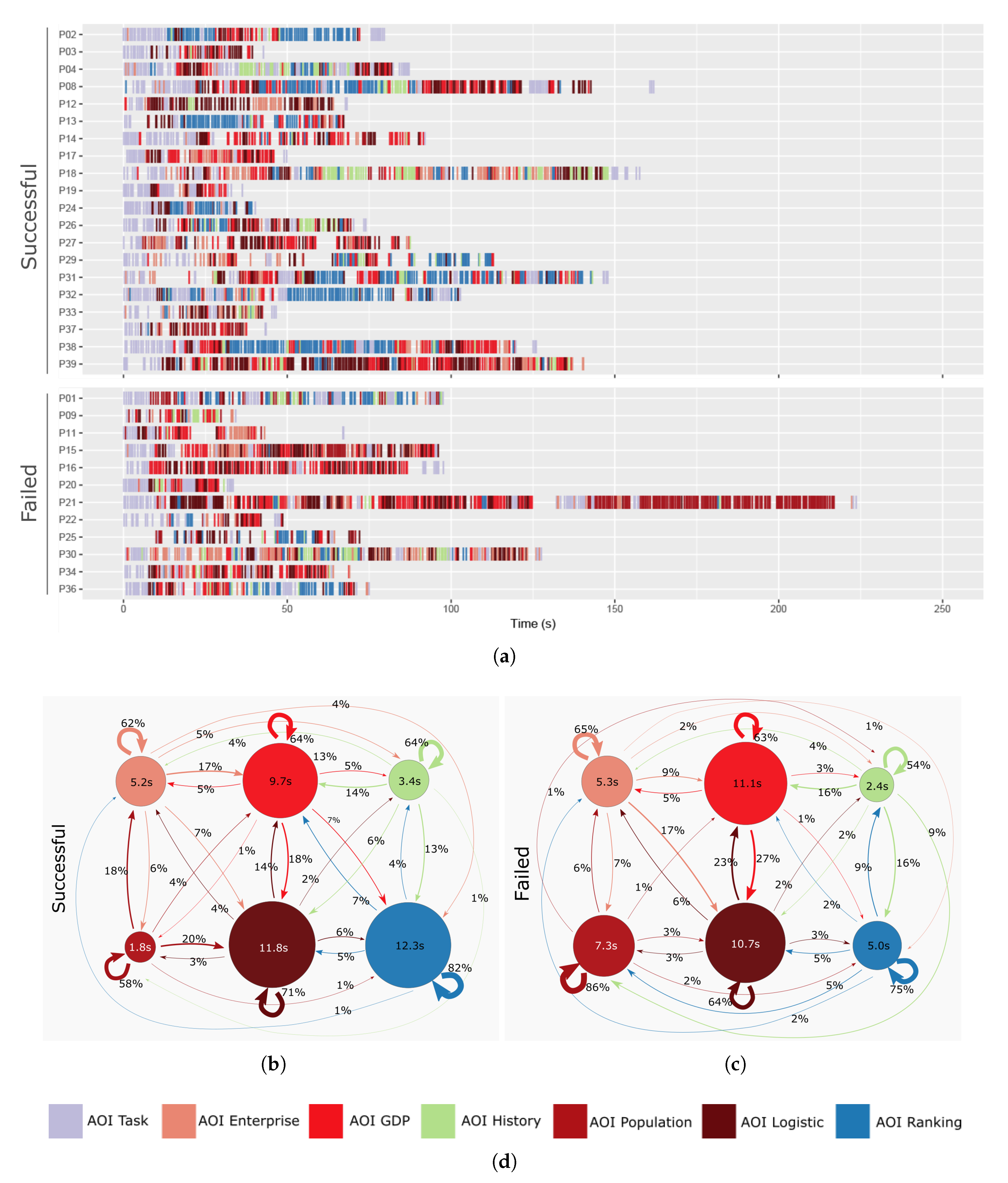
We explain these five themes in detail. (1) The attraction on the dashboard panels was well reflected by the visual fixation on the dashboard during the free-exploration stage. To show the attention distribution, we visualized the fixation positions in the first 90 seconds using heatmaps. (2) The effectiveness is measured by the task-solving correctness. We compared the success rates in solving the benchmark tasks first among the different cognitive complexities, second among the increasing familiarity of the proposed dashboard, and finally among different participant groups. More specifically, we assumed that the familiarity of the proposed dashboard increases while the participants were carrying out the tasks. (3) We measured the efficiency using the response time of completing a task. The duration of each task-solving step was recorded between the starting click and the ending click. Similarly, the response time was also compared according to different cognitive complexities, the familiarity of the proposed dashboard, and different participant groups. In addition, the response time was compared between the successfully and unsuccessfully performed tasks. (4) The search strategies of the participants were measured. These were comprised of the search sequence, average dwell time, and the transition and return probabilities among the Areas of Interest (AOIs) in each task. According to [39], we listed the selected metrics of the eye movements in Table 3. We selected seven AOI areas on the dashboard shown in Figure 5, including Task, AOI Enterprise, AOI GDP, AOI History, AOI Population, AOI Logistic, and AOI Ranking. Since we focused on how the participants construct knowledge via multiple panels, the AOIs were selected based on the dashboard panels and their contents. The spatial panel was divided into four AOIs, as each map shows different categories of data. Moreover, these metrics were visually analyzed. The sequences of the fixations on the AOIs were visualized in sequence charts, with each fixation shown as a color block along the timeline. Based on the visualization method of transition states proposed in [40], we designed a dwell and transition chart to show the eye movement patterns between the AOIs. In this chart, each AOI is represented by a circle, and the radius stands for the average dwell. The transition between two AOIs is represented by a line, and the width stands for the transition probability. (5) The attitude of participants is reflected by their answers from the interview. The confidence rates and overall usability rates were qualitatively analyzed. The positive and negative design items listed by the participants were grouped in the dashboard panel, layout, interaction, and others.
4. Evaluation Results
This section describes the analysis results of the eye movement data and the interview feedback collected from the experiment. More specifically, we introduce the results in the following five aspects: (1) The participants’ fixations in free exploration; (2) success rate; (3) response time; (4) the participants’ fixation, dwell, and transition of the AOIs during their task-solving stages; (5) the feedback from the participants. The eye-tracking data is published online (https://github.com/Map-based-Dashboard/eye-tracking-experiment).
4.1. Fixation in Free Exploration
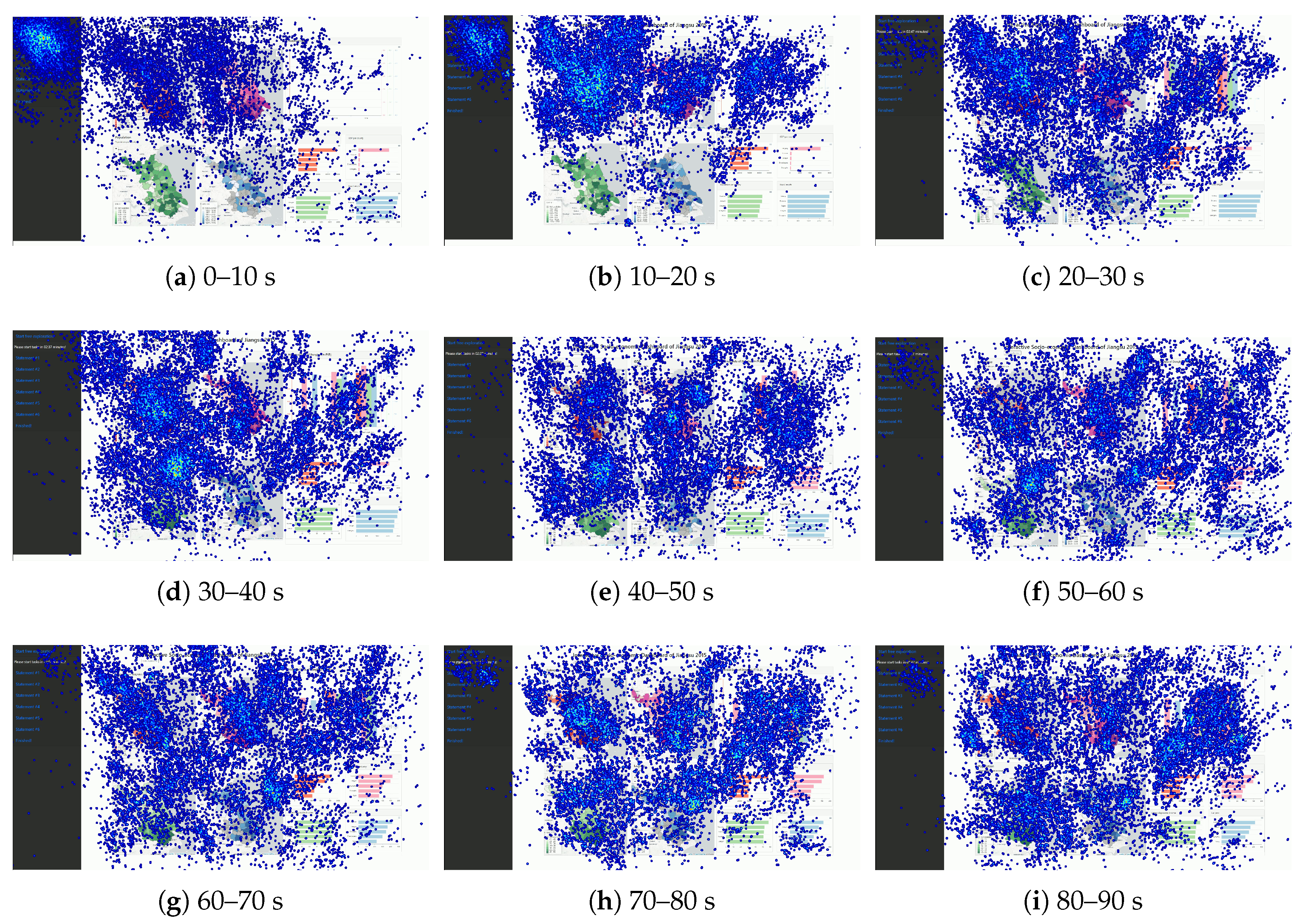
The fixation distribution of the participants reflects the visual attraction of different sections of the visual interface. We show the fixation distribution in the first 90 s at the free exploration stage on heatmaps (shown in Figure 6). Considering our sample size, we chose 10 s as the interval to include enough fixations in forming clusters in each interval. The heatmaps exhibit different patterns of the fixation distribution in 0–20 s (Figure 6a,b) and 20–90 s (Figure 6c–i). In the first 10 s (Figure 6a), we can see that the fixations were mostly on the title, AOI Task, AOI Enterprise, and AOI GDP. Between 10 to 20 s (Figure 6b), the fixations were more on AOI Enterprise, AOI GDP, AOI History, and less on AOI Task. From 20 to 90 s (Figure 6c–h), the attention of the participants was located more evenly on each dashboard panel. In general, panels located in the center attracted more attention than other panels at the free exploration stage, for example, AOI Enterprise and AOI GDP were focused on at the beginning of the exploration, while AOI Ranking only received a small amount of attention. The visualizations with a high information density also attracted more attention from the participants, because there were more fixations on the maps than on the bar charts. The dynamic visualizations attracted a significant amount of attention. For example, the AOI History drew a large amount of attention, as the chart in the panel changed when there was a mouse hover or click. In contrast, AOI Ranking did not involve much interaction and it received less attention. Additionally, a large amount of attention went to AOI Task in the beginning because the participants needed to click and read the task items. We inferred that bright colors also play an important role in attracting users’ attention. Last but not least, anomalous patterns, such as incomplete data and outliers, also attracted the participants’ attention. In the 0–30 s, more fixations were at the AOI Logistic than AOI Population, where a large gray area indicated unavailable data.
4.2. Success Rate
The success rate reflects the effectiveness of the dashboard design. In this section, we first compared the success rates according to the perception difficulties of the tasks and the familiarities of the proposed dashboard of the participants. Specifically, we compared the success rates among the proposed benchmark tasks (Section 3.3). The levels of difficulty in perception raised from the tasks T1 to T6. The familiarity levels of the dashboard increased from the statements S1 to S6 on the experiment tool (Section 3.4). Recall that the experiment tool shows each participant the tasks in random order. We assume that the participants were becoming familiar with the dashboard while they were carrying out the tasks.
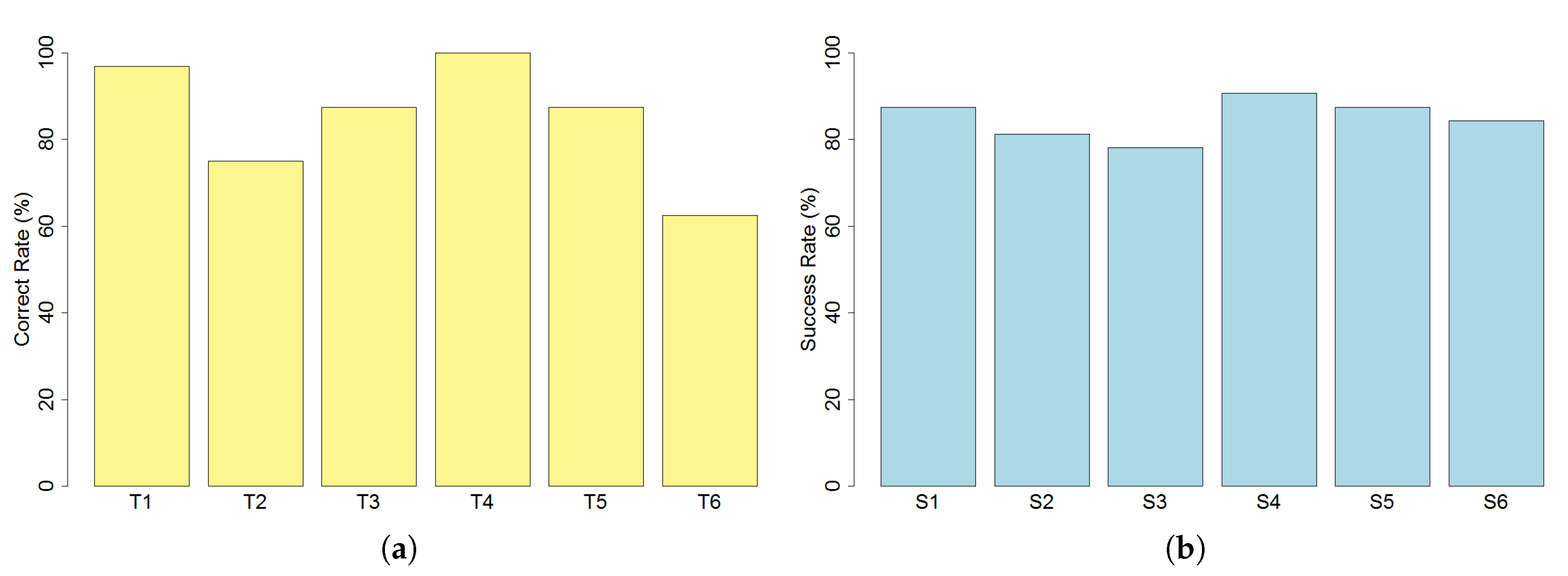
Figure 7 shows the success rates according to the order of increasing difficulty (from T1 to T6) (Figure 7a) and the order of increasing familiarity (from S1 to S6) (Figure 7b). From Figure 7a, we can see that in general the success rates are very high for all the tasks. Among the identification tasks from T1 to T3, we can see that T1 and T3 have higher success rates than T2. Compared to T2, T1 requires a lower cognitive effort than T2 and more dashboard interactions, while T3 requires less dashboard interaction and more complex cognitive operation. For the reasoning tasks from T4 to T6, the success rates decrease significantly. Figure 7b shows in general the success rates did not increase with the participants’ familiarity with the dashboard.
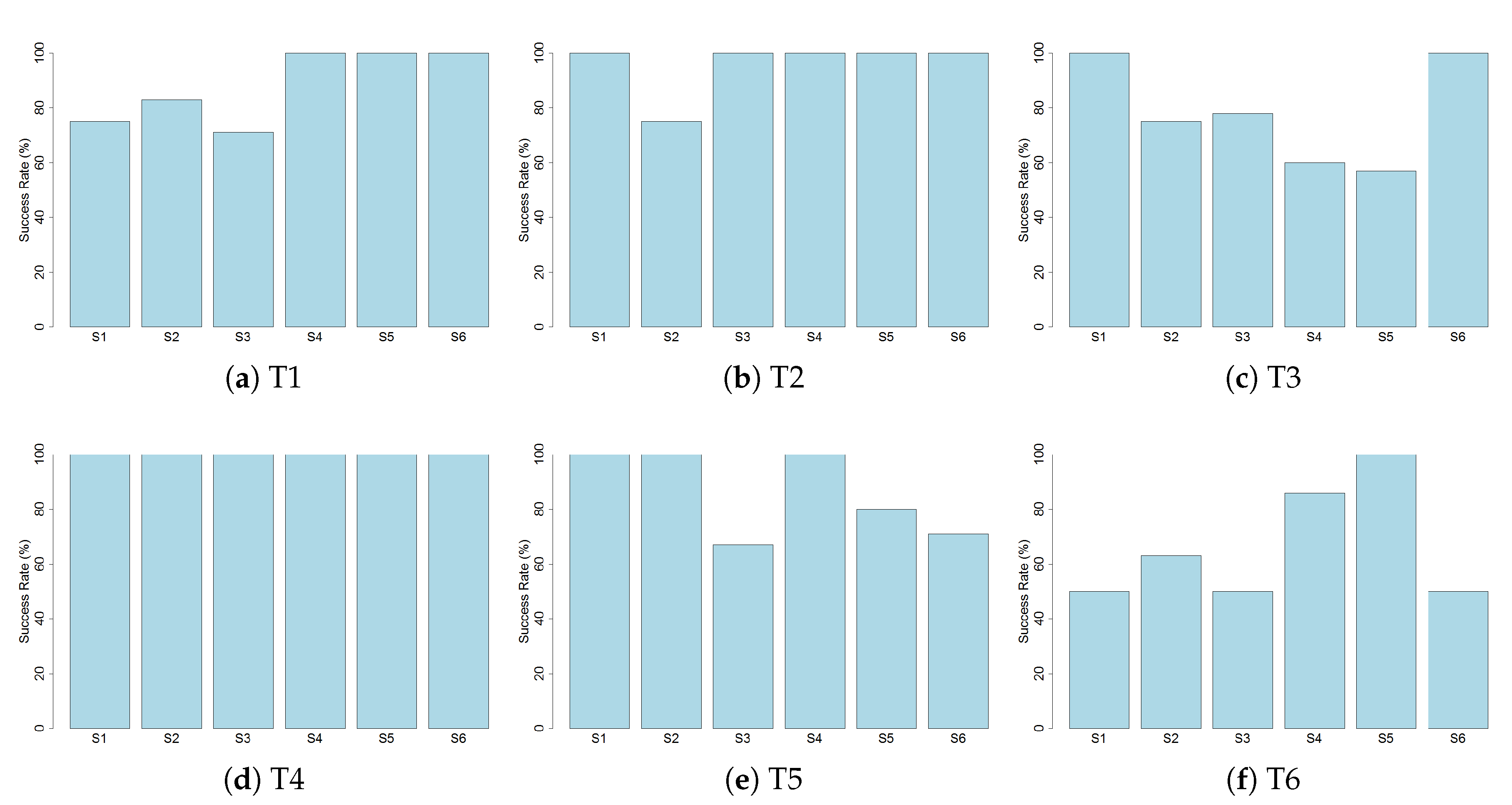
Figure 8 further shows the success rates of each task across the position of the task sequence. The success rates of T3–T6 did not increase along with the increasing of the familiarity of the dashboard. However, the success rates of T1 and T2 had an upward trend. It might indicate that the participants were performing better in location searching when they became more familiar with the dashboard.
Finally, we compared the success rates among different groups of participants including aspects such as gender, educational background, and usage experience. Table 4 shows the success rates of each task of different groups. Most of the tasks were correctly conducted in every group. The average success rate of all the participants is 84.9%. The success rates did not show great differences among these groups.
4.3. Response Time
To analyze the efficiency of the dashboard, we examined the response time in completing the tasks. Similar to the success rate analysis, we compared the median response time first among the increasing cognitive complexities, second among the increasing familiarities of the dashboard, and third among the different participant groups. Additionally, we compared the response time between the successful and failed tasks.
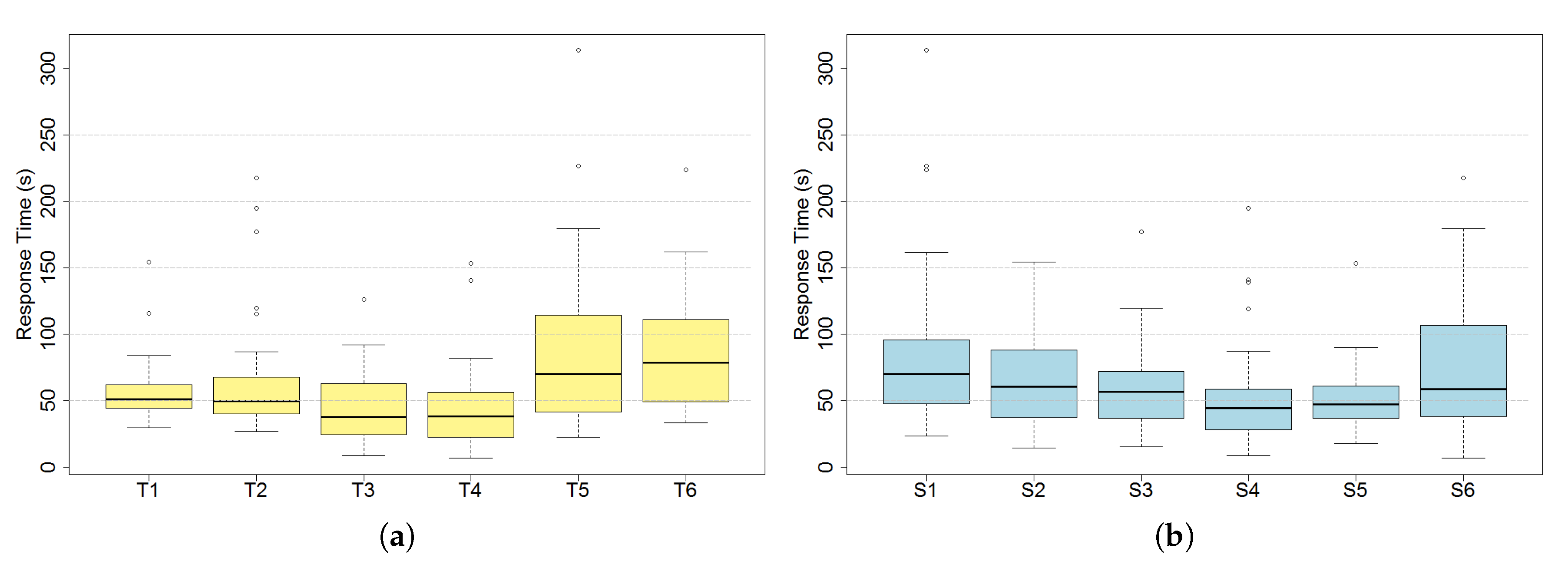
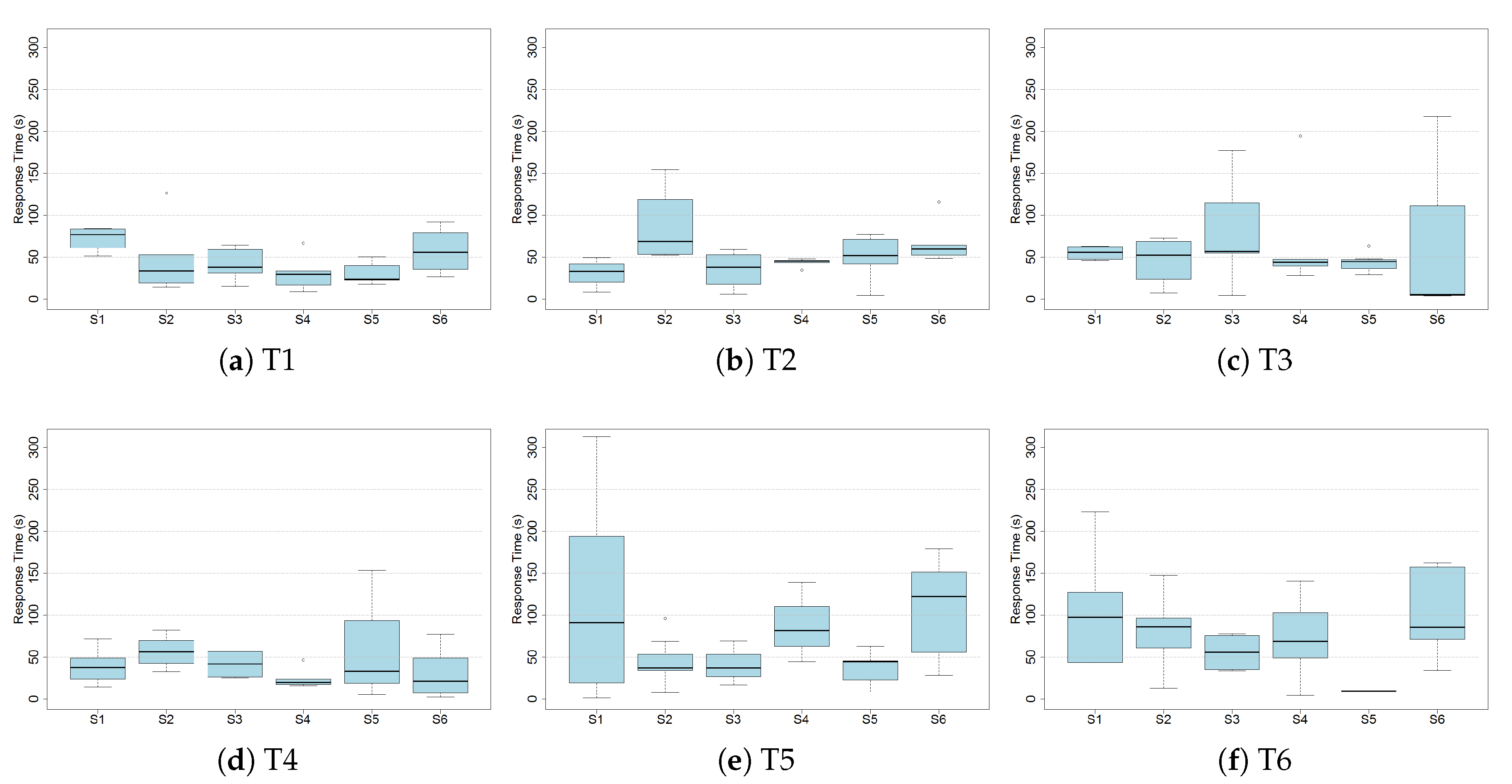
Figure 9 uses boxplots to show the response time of each task. The median response time of all the tasks was 51.5 s. In Figure 9a, we can see that all the identification tasks (T1–T3) took relatively less time, while the respond time of reasoning tasks (T4–T6) varied a lot. The response time of T5 and T6 was much longer and more dispersed than T4. Figure 9b shows a general downward trend of the response time along the increasement of the familiarity. This could indicate that the more the participants interact with the dashboard, the shorter the time they need to solve a task. The median response time did not continue to decrease after the completion of four tasks. It might indicate that the participants were familiar enough with the dashboard after carrying out the first four tasks, and the median duration was 3.9 min. The median response time of the last two completed tasks was at a relatively low level, but the increasing variation might suggest that some of the participants were tired towards the end of the experiment.
Figure 10 shows in detail the response time of each task in the carried out sequence. We cannot see an obvious downward trend from each task, which could be caused by the small sample size. However, we can see that T5 and T6 had a relative longer response time when they were carried out in the first position.
Table 5 gives an overview of the median response time of each task in different groups. We found that the response time does not exhibit many differences among groups with different demographic attributes.
The differences in response time between the successful and failed tasks is shown in Figure 11. The figure shows that except for T6, the median response time of the failed tasks is longer than the successful ones. This could indicate that the failed tasks were caused by the wrong search strategy of the participants.
4.4. Dwell and Transition during Tasks
To find more differences in the task-solving strategies between the successful and failed tasks, we compared the fixation sequences, as well as the dwell and transitions in performing the tasks. For each task, we illustrated the fixation sequence of the participants in sequence charts, using the same color scheme of the AOIs in Figure 5. The time range of the sequence charts was set as 0–250 seconds as it fits well to all the tasks, so that we can better compare the fixation among the tasks. From the sequence charts, we could easily interpret the fixation time and the viewing orders of AOIs of each individual participant. We also visualized the average dwell time and transition probabilities among AOIs for each task. In all the sequence charts and the dwell and transition charts, the successful and failed groups are visualized separately. For each task, we described the most effective solution and compared the participants’ solutions with it. In this section, we examine in detail the strategies of the participants in solving the tasks with the aim of identifying clues on how to improve further the effectiveness and efficiency of the dashboard.
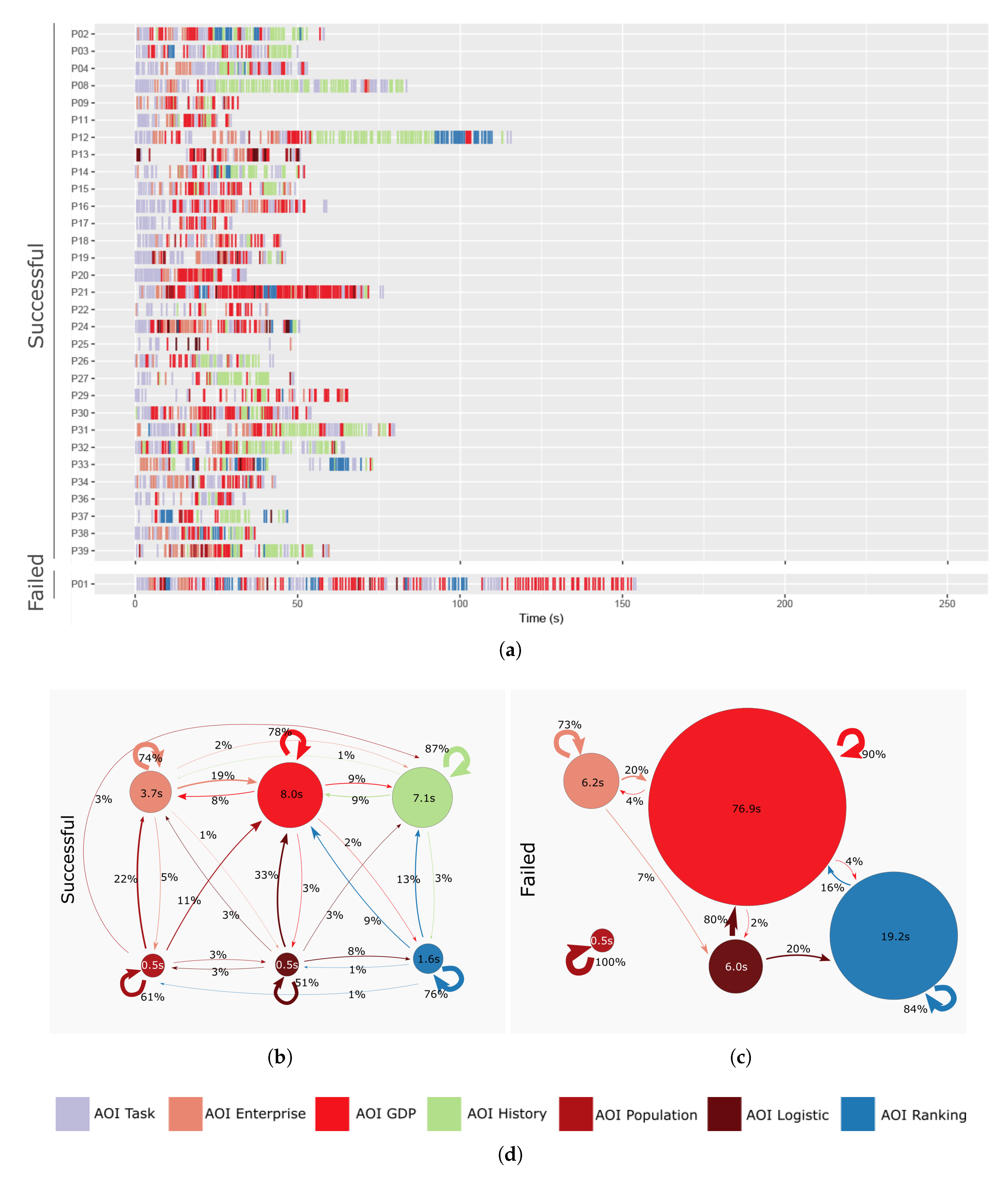
For T1 “In 2015, the Tertiary Industry value of Qidong is 85 billion CNY. (Wrong)”, the participants needed to find a GDP-related value of a county. To solve it, the most effective solution was to (1) locate County Qidong with the search function, (2) switch the layer to Layer Tertiary Industry in AOI GDP, and (3) move the mouse onto AOI GDP or AOI History to read the value in the pop-up window. As shown in Figure 12, the participants spent most of the time in checking AOI GDP and AOI History. The failed user was spending a lot of time on AOI Ranking, which did not provide the needed information. We found that the viewing in the combination of AOI GDP and AOI Task often happened shortly before some participants (P2, 4, 14, 17, 19, 31, 36) finished the task. This indicates that when the participants knew where to find the ranking information, they can quickly finish the task.
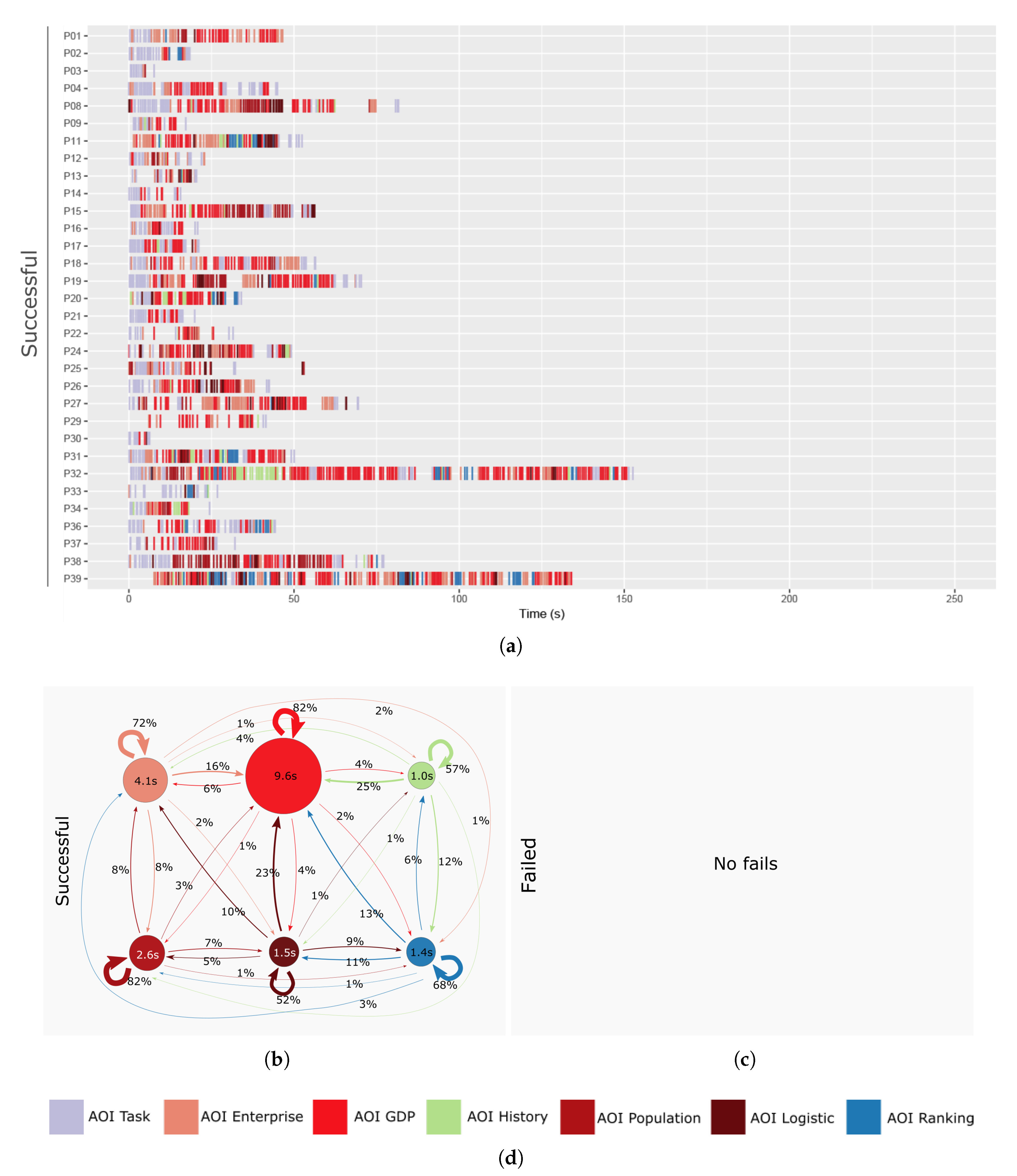
For T2 “The number of enterprises in Jintan increases from 2013 to 2015. (Unknown)”, it required the participants to find the temporal trend of an enterprise-related factor of a county. To solve T2, the best solution was to (1) locate Jintan with the search function, (2) make sure the active layer is Enterprise in the Enterprise category, and (3) read the temporal trend of number of enterprises in the bar chart on AOI History. From Figure 13, we can see that the participants spent the most time on viewing AOI Enterprise and AOI Ranking. This is because they were using the search bar to locate the place in the task. Some participants (P1, 3, 22) spent relatively longer time on AOI Enterprise and AOI History, and most of the transitions are from AOI GDP. It suggests that they were having difficulties in solving step (1) and (3) of this task.
T3 “In 2015, among all the counties in Jiangsu, Kunshan has the largest number of enterprises. (Correct)” required the participants to find the county with the highest value of an enterprise-related factor. The most effective solution was (1) make sure the active layer was the Layer Enterprise in AOI Enterprise, and (2) read the name of the top county on AOI Ranking. Figure 14 shows that the participants were mainly paying attention to view the AOI Enterprise. They used the search bar in the AOI Enterprise to locate the place, and checked the AOI Ranking and the AOI History. The AOI Ranking took on average only 3 seconds in the successful group. This may indicate that the view was efficient. However, two of the four failed participants (P22, 25) completely missed the AOI Ranking. This suggests that the two participants were not familiar with the dashboard interface.
T4 “The south part of Jiangsu is economically stronger than the north part. (Correct)” required the participants to find a GDP-related factor’s spatial distribution. Its effective solution was to check the spatial distribution of the layers in AOI GDP. From Figure 15, we can see that all the participants finished the task quickly and successfully. Most of the time, the participants were viewing AOI GDP. From the transitions chart, we infer that the participants knew where to find the spatial distribution information. Two participants (P3 and P30) finished T4 within 10 seconds with the search strategy of first reading the statement, then viewing the related information in AOI GDP, and then confirming their answers by rereading the statement again.
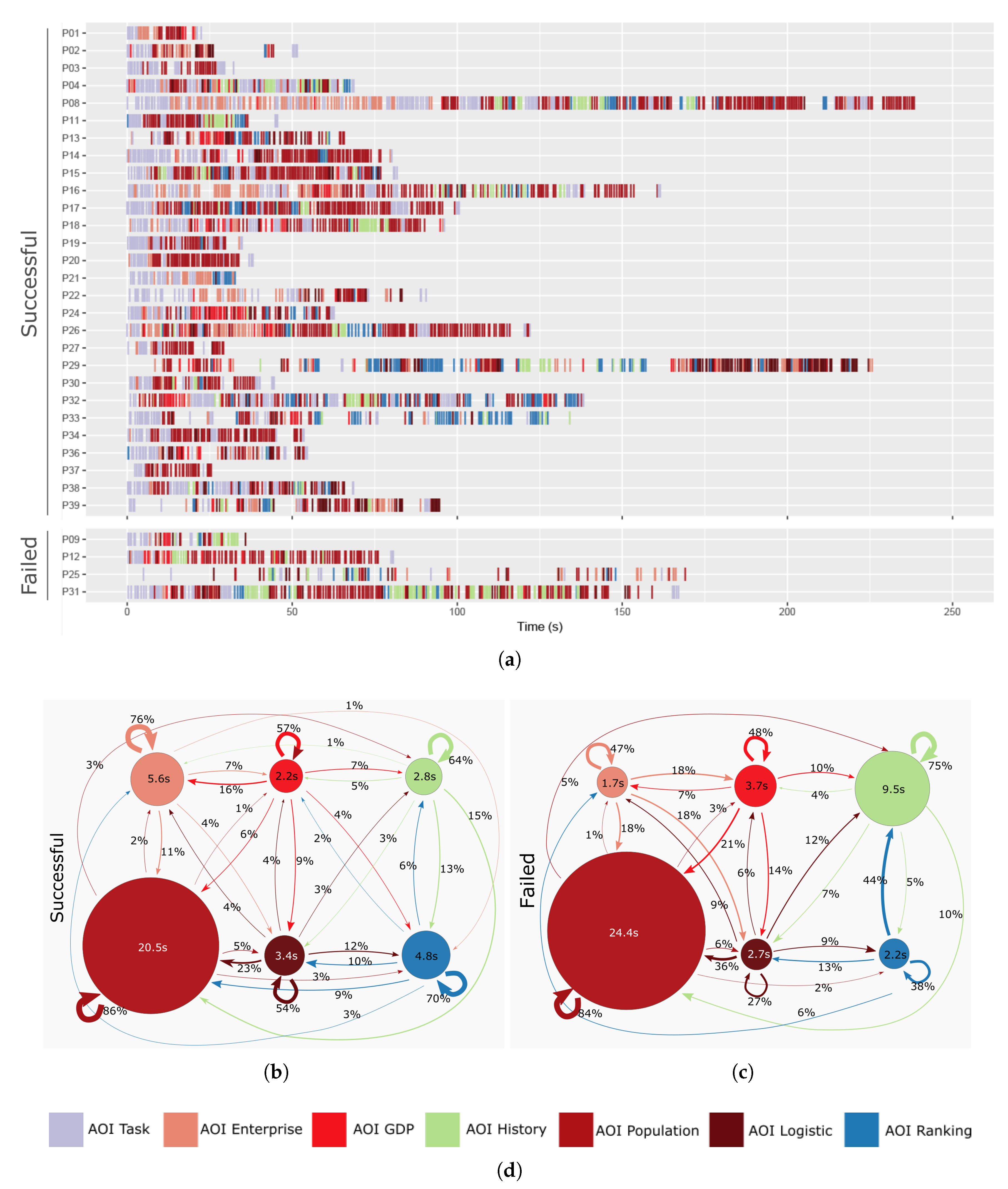
T5 “In Jiangsu, the more employees in a county, the higher the citizens’ disposable income is. (Wrong)” required the participants to compare the spatial correlation between two population-related factors. The effective solution was to compare the spatial distributions between the Layer Employee and the Layer Citizen disposable income in the AOI Population. As seen from Figure 16, both successful and failing groups focused on the AOI Population to check the spatial correlation. A few participants (P29, 32, and 33) checked AOI Ranking for some time. Some participants (P16, 31, and 32) viewed AOI History for some time. We infer that the participants knew where to find the answers on the dashboard, but the high perception difficulty caused a longer viewing time.
T6 “In Jiangsu, the longer the total length of the road of a county, the higher the industrialized level is. (Wrong)” required the participants to find the correlation between a logistics-related factor and a GDP-related factor, and the data of the logistics-related factor were incomplete. The most effective solution for T6 was to compare the spatial distribution between the Layer Road length in the AOI Logistic and the Layer Secondary industry in the AOI GDP. From Figure 17, we can see that the participants were comparing AOI Logistic and AOI GDP. Some participants were trying to find the correlation by comparing the factors in AOI Ranking, which was a wrong strategy. The unavailable data required the participants to summarize the correlation with less data than T5, which was more challenging and thus caused more failed cases.
In summary, the reading sequence during the task solving is mainly driven by two reasons. One reason is the task requirement. The participants viewed the dashboard focused on searching for the most relevant information required by the tasks. Therefore, labeling of the panels is very important in navigating the users’ attention to the needed information. Another reason is the layout of the panels. The participants tended to read the adjacent panel after reading the current panel. Thus the layout of the panels plays an important role in dashboard reading.
4.5. Feedback
In this section, we evaluated the usability of the dashboard by analyzing the feedback from the interview. First, we discussed the rating of the participants on the usability of the dashboard. Second, we classified the keywords in the interview protocol in groups of dashboard design elements.
The participants rated on average 8.25 (1–10 from less to more confident) on the confidence of their answers, and 7.89 (1–10 from very hard to very easy to use) on the general usability of the dashboard. The overall results were very positive. Moreover, some of the participants reported they were less confident with the answers of T5 and T6. There were two reasons for this: one was that the unavailable data made them unsure of their answers, and the other one was because of the lack of economic knowledge background.
We asked the participants to list the design items that helped them during the task-solving procedure without predefined options. The feedback is grouped into four categories: panel, layout, interaction, and others. Table 6 summarizes the positive feedback with the associated frequency in each group. In the panel group, the most helpful panel was the spatial panel (nine mentions). In the layout group, the color scheme was very helpful in supporting the participants in organizing the information. In the interaction group, the search function was identified as the most helpful item.
Similarly, we have grouped the negative design items named by the participants in the interview. Table 7 shows the items in detail. Compared to the positive items, the negative ones are more related to specific issues. The most frequently mentioned items are the top margin of the bars in the temporal panel is sometimes too narrow, the shifting of the maps is disturbing, and the font size is too small. It is important to note that three participants thought the temporal panel is too informative, and one participant pointed out the temporal panel did not follow the four category structure as other panels did. Two participants also commented that they did not know where to look for the information that they needed.
In summary, map-based dashboards are very useful media to show the spatiotemporal information. Maps are the main element to bridge the knowledge from different perspectives and their location information. A uniformed style (color scheme, interaction, layout) of all the panels can help the users in dashboard reading.
5. Discussion
In this section, we discuss the strengths and weaknesses of the proposed map-based dashboard for spatiotemporal knowledge acquisition and analysis, and the limitations of the experiment.
The map-based dashboard is designed to enable users to acquire and analyze spatiotemporal knowledge. The panels are designed to reveal different perspectives of georeferenced knowledge about what happens where and how it happens. The linked panels provide users with the real-time response of the subsets of the data. Each panel is placed on a fixed position and outlined with an enclosure, giving users a necessary anchor to quickly navigate in the data space. The juxtaposition reduces the difficulties in comparing multiple factors and facilitates the correlation analysis. The arrangement of the panels is very important. We placed the spatial panel in the middle area and in a large size to guide the users’ attention to it. Last but not least, we applied a uniformed design style (color, layout, interaction) to each panel with the aim to foster the habit formation for an efficient perception and interaction.
However, the current design can be improved in some aspects. The annotations in dashboards have not received sufficient attention in previous studies. We realized that the font plays a very important role in dashboard understanding. The font size should be big enough to read at a glance. To better guide users to visually explore the data, the labeling of the panels should clearly express what types of information it conveys. Therefore, the panels in our dashboard should be labeled as the spatial panel, temporal panel, and ranking panel. Furthermore, the arrangement of panels should follow a logical order. The panels with similar content should be placed adjacently. When visualizing multi-granularity or multi-temporal data in several panels, the sequence of the panels should follow a common reading pattern, such as from large to small, or from old to new. Moreover, the function of each panel should remain simple. In this dashboard, we should integrate the search and layer switch functions to the toolbar. In addition, the design style of each panel should be kept uniform. The temporal panel should be split into four charts, as in the spatial and ranking panel. The clicking and hovering function should also be designed in the ranking panel. Moreover, we should prepare a second color scheme for the color-blind users.
The evaluation experiment of the dashboard has led to some new insights. Compared to similar experiments with only interviews in [18] or only an eye-tracking experiment in [35], our eye movement data and the interview provide complementary results reflecting the user experience and the usability of the map-based dashboard. With regard to the sample size of participants, 40 participants divided into smaller groups may seem to be small, but it is still an acceptable sample size. In similar eye-tracking experiments, the number of participants was usually not large, e.g., 21 and 17 participants in [25,35]. Our dashboard has been experimentally proved both effective and efficient for different groups. In future studies, more people with economics-related background or domain experts will be invited. Another insight is related to how feedback was collected. We adopted semi-structured interviews, and the participants were asked to list the positive and negative design items. Although the interviews were carried out immediately after the experiment, the participant tended to ignore some items or focus on the last issues they encountered prior to ending their participation. One alternative to this problem is to use a predefined questionnaire to measure each design item as suggested by Pezanowski et al. [17]. Think-aloud would be another method as a complement during the experiment [7]. It can allow participants to talk more about how they made their decisions in answering the benchmark tasks.
6. Conclusions
Map-based dashboards have opened up convenient opportunities for stakeholders to perceive and analyze complex spatiotemporal knowledge from multi-dimensional data with an at-a-glance overview and details on demand. By integrating the high-interactive and high intuitive features of visual analytics into the dashboard, we expanded the dashboard with more analytical functions. Moreover, we have contributed the design lessons of map-based dashboards.
In this study, we designed and developed a map-based dashboard displaying geo-economic environmental data targeting decision-makers in SMEs and citizens. To evaluate the effectiveness and efficiency of our map-based dashboard, we specially designed an experiment consisting of an eye-tracking study, benchmark tasks, and an interview. We analyzed the collected eye movement data in terms of fixation, success rate, response time, and dwell and transition metrics. Furthermore, we analyzed the feedback and summarized the positive and negative items on views, layout, interaction, and others. The analysis results from the eye-tracking study and the interviews have verified the map-based dashboard for spatiotemporal knowledge acquisition along with a number of findings related to the limitations of the current design of map-based dashboards and user studies.
Our future work involves three main tasks. First, the interface design will be improved with the focus on the study of how different layouts of the multiple views and their labeling influence the efficiency of the corresponding dashboards. Second, further user experience and usability experiments will be conducted. We will quantitatively study how the visualization, panel arrangement, color scheme, and user background influence users’ attention and the spatiotemporal knowledge acquisition and analysis. Lastly, we will extend our dashboard design by adding more visual analytical methods. For instance, we will add correlation calculation and anomaly detection function and dashboard panels. We also plan to conduct more experiments on different datasets, e.g., social media data and volunteered geographic information.
Author Contributions
Conceptualization, Chenyu Zuo, Linfang Ding and Liqiu Meng; methodology, Chenyu Zuo; software, Chenyu Zuo; Formal analysis, Chenyu Zuo; investigation, Chenyu Zuo; resources, Chenyu Zuo; data curation, Chenyu Zuo; writing—original draft preparation, Chenyu Zuo; writing—review and editing, Chenyu Zuo, Linfang Ding and Liqiu Meng; visualization, Chenyu Zuo; supervision, Linfang Ding and Liqiu Meng; project administration, Chenyu Zuo and Linfang Ding. All authors have read and agreed to the published version of the manuscript.
Funding
This work is funded by the project “A Visual Computing Platform for the Industrial Innovation Environment in Yangtze River Delta” supported by the Jiangsu Industrial Technology Research Institute (JITRI) and Changshu Fengfan Power Equipment Co., Ltd.
Acknowledgments
The census and land use datasets are provided by Yangtze River Delta Science Data Center, National Earth System Science Data Sharing Infrastructure, National Science & Technology Infrastructure of China (http://nnu.geodata.cn:8008/). The authors would also like to thank the editor and anonymous reviewers for their efforts to review this paper.
Conflicts of Interest
The authors declare no conflict of interest.
Abbreviations
The following abbreviations are used in this manuscript:
| AOI | area of interest |
| CEO | chief executive officer |
| SME | small and medium-sized enterprise |
| GDP | gross domestic product |
| CNY | Chinese Yuan |
Appendix A

Table A1.
The selected socioeconomic factors and the statistics of the data.
| Category | Factor | Explanation |
|---|---|---|
| Enterprise | Enterprise | The total number of the enterprises in a county |
| Enterprise above designated size | The number of enterprises with annual main business revenue of 20 million CNY or more | |
| GDP | GDP per county | The total gross domestic product in one county |
| GDP per capita | The average GDP per person | |
| Primary industry | The GDP value of the county from natural raw materials, such as mining, agriculture, or forestry | |
| Secondary industry | The GDP value of industry which converts the raw materials provided by primary, such as manufacturing industry | |
| Tertiary industry | The GDP value concerned with the provision of services | |
| Population | Population per county | The total population of one county |
| Population per km2 | The population density of one county | |
| Employee | The total number of employees in one county | |
| Citizen disposable income | The average citizen disposable income of one county | |
| Citizen consumption | The average citizen consumption of one county | |
| Engel coefficient | The proportion of income spent on food falls | |
| Logistic | Road length | The total road length in one county |
| Road passenger | The total transported passenger number in one county in one year | |
| Road cargo | The total weight of the transported cargo in one county in one year | |
| Car parc | The number of cars and other vehicles in a region or market |
References
- Jing, C.; Du, M.; Li, S.; Liu, S. Geospatial Dashboards for Monitoring Smart City Performance. Sustainability 2019, 11, 5648. [Google Scholar] [CrossRef] [Green Version]
- Few, S. Information Dashboard Design: The Effective Visual Communication of Data; O’Reilly Media, Inc.: Newton, MA, USA, 2006. [Google Scholar]
- Huijboom, N.; Van den Broek, T. Open data: An international comparison of strategies. Eur. J. ePractice 2011, 12, 4–16. [Google Scholar]
- Kitchin, R.; Lauriault, T.P.; McArdle, G. Knowing and governing cities through urban indicators, city benchmarking and real-time dashboards. Reg. Stud. Reg. Sci. 2015, 2, 6–28. [Google Scholar] [CrossRef] [Green Version]
- Liu, Z.; Jiang, B.; Heer, J. imMens: Real-time Visual Querying of Big Data. Comput. Graph. Forum 2013, 32, 421–430. [Google Scholar] [CrossRef] [Green Version]
- Reda, K.; Johnson, A.E.; Papka, M.E.; Leigh, J. Effects of Display Size and Resolution on User Behavior and Insight Acquisition in Visual Exploration. In Proceedings of the 33rd Annual ACM Conference on Human Factors in Computing Systems (CHI ’15), Seoul, Korea, 18–23 April 2015; Association for Computing Machinery: New York, NY, USA, 2015; pp. 2759–2768. [Google Scholar] [CrossRef] [Green Version]
- Yalçın, M.A.; Elmqvist, N.; Bederson, B.B. Keshif: Rapid and Expressive Tabular Data Exploration for Novices. IEEE Trans. Vis. Comput. Graph. 2018, 24, 2339–2352. [Google Scholar] [CrossRef] [PubMed]
- Vornhagen, H. Effective visualisation to enable sensemaking of complex systems. The case of governance dashboard. In Proceedings of the International Conference EGOV-CeDEM-ePart, Donau, Austria, 3–5 September 2018; pp. 313–321. [Google Scholar]
- Gurstein, M.B. Open data: Empowering the empowered or effective data use for everyone? First Monday 2011, 16. [Google Scholar] [CrossRef]
- Batty, M.; Axhausen, K.W.; Giannotti, F.; Pozdnoukhov, A.; Bazzani, A.; Wachowicz, M.; Ouzounis, G.; Portugali, Y. Smart cities of the future. Eur. Phys. J. Spec. Top. 2012, 214, 481–518. [Google Scholar] [CrossRef] [Green Version]
- Batty, M. A perspective on city dashboards. Reg. Stud. Reg. Sci. 2015, 2, 29–32. [Google Scholar] [CrossRef] [Green Version]
- Census Mappong Module: Dublin City. Available online: http://airo.maynoothuniversity.ie/Instant_Atlas/Updated%20Modules/dd/Dublin%20City/atlas.html (accessed on 25 June 2020).
- Smart City 2-Boston Smartcity. Available online: https://boston.opendatasoft.com/page/smart-city-2/ (accessed on 25 June 2020).
- Visualising Enterprise, Innovation & Employment in Galway City and County. Available online: http://galwaydashboard.ie/enterprise (accessed on 25 June 2020).
- Keim, D.; Andrienko, G.; Fekete, J.D.; Görg, C.; Kohlhammer, J.; Melançon, G. Visual Analytics: Definition, Process, and Challenges. In Information Visualization: Human-Centered Issues and Perspectives; Kerren, A., Stasko, J.T., Fekete, J.D., North, C., Eds.; Springer: Berlin/Heidelberg, Germany, 2008; pp. 154–175. [Google Scholar] [CrossRef] [Green Version]
- Robinson, A.C.; Peuquet, D.J.; Pezanowski, S.; Hardisty, F.A.; Swedberg, B. Design and evaluation of a geovisual analytics system for uncovering patterns in spatio-temporal event data. Cartogr. Geogr. Inf. Sci. 2017, 44, 216–228. [Google Scholar] [CrossRef]
- Pezanowski, S.; MacEachren, A.M.; Savelyev, A.; Robinson, A.C. SensePlace3: A geovisual framework to analyze place–time–attribute information in social media. Cartogr. Geogr. Inf. Sci. 2018, 45, 420–437. [Google Scholar] [CrossRef]
- Li, J.; Chen, S.; Zhang, K.; Andrienko, G.; Andrienko, N. COPE: Interactive Exploration of Co-Occurrence Patterns in Spatial Time Series. IEEE Trans. Vis. Comput. Graph. 2019, 25, 2554–2567. [Google Scholar] [CrossRef] [PubMed]
- Nazemi, K.; Burkhardt, D. Visual analytical dashboards for comparative analytical tasks—A case study on mobility and transportation. Procedia Comput. Sci. 2019, 149, 138–150. [Google Scholar] [CrossRef]
- Roth, R.E. Interactive maps: What we know and what we need to know. J. Spat. Inf. Sci. 2013, 2013, 59–115. [Google Scholar] [CrossRef]
- Roth, R.E.; Çöltekin, A.; Delazari, L.; Filho, H.F.; Griffin, A.; Hall, A.; Korpi, J.; Lokka, I.; Mendonça, A.; Ooms, K.; et al. User studies in cartography: Opportunities for empirical research on interactive maps and visualizations. Int. J. Cartogr. 2017, 3, 61–89. [Google Scholar] [CrossRef]
- Chang, R.; Ziemkiewicz, C.; Green, T.M.; Ribarsky, W. Defining Insight for Visual Analytics. IEEE Comput. Graph. Appl. 2009, 29, 14–17. [Google Scholar] [CrossRef]
- Roth, R.E.; Ross, K.S.; MacEachren, A.M. User-Centered Design for Interactive Maps: A Case Study in Crime Analysis. ISPRS Int. J. Geo-Inf. 2015, 4, 262–301. [Google Scholar] [CrossRef]
- Andrienko, N.; Andrienko, G.; Gatalsky, P. Exploratory spatio-temporal visualization: An analytical review. J. Vis. Lang. Comput. 2003, 14, 503–541. [Google Scholar] [CrossRef]
- Bogucka, E.; Jahnke, M. Feasibility of the Space–Time Cube in Temporal Cultural Landscape Visualization. ISPRS Int. J. Geo-Inf. 2018, 7, 209. [Google Scholar] [CrossRef] [Green Version]
- Brinck, T.; Gergle, D.; Wood, S.D. Usability for the Web: Designing Web Sites That Work; Morgan Kaufmann Publishers: Burlington, MA, USA, 2001. [Google Scholar]
- Brooke, J. SUS: A “quick and dirty’usability. In Usability Evaluation in Industry; Routledge: Abingdon, UK, 1996; p. 189. [Google Scholar]
- Seebacher, D.; Häuäler, J.; Hundt, M.; Stein, M.; Müller, H.; Engelke, U.; Keim, D. Visual Analysis of Spatio-Temporal Event Predictions: Investigating the Spread Dynamics of Invasive Species. IEEE Trans. Big Data 2018. [Google Scholar] [CrossRef] [Green Version]
- Cao, N.; Lin, C.; Zhu, Q.; Lin, Y.; Teng, X.; Wen, X. Voila: Visual Anomaly Detection and Monitoring with Streaming Spatiotemporal Data. IEEE Trans. Vis. Comput. 2018, 24, 23–33. [Google Scholar] [CrossRef]
- Liu, D.; Xu, P.; Ren, L. TPFlow: Progressive Partition and Multidimensional Pattern Extraction for Large-Scale Spatio-Temporal Data Analysis. IEEE Trans. Vis. Comput. Graph. 2019, 25, 1–11. [Google Scholar] [CrossRef] [PubMed]
- Shi, L.; Huang, C.; Liu, M.; Yan, J.; Jiang, T.; Tan, Z.; Hu, Y.; Chen, W.; Zhang, X. UrbanMotion: Visual Analysis of Metropolitan-Scale Sparse Trajectories. IEEE Trans. Vis. Comput. Graph. 2020. [Google Scholar] [CrossRef]
- McKenna, S.; Staheli, D.; Fulcher, C.; Meyer, M. BubbleNet: A Cyber Security Dashboard for Visualizing Patterns. Comput. Graph. Forum 2016, 35, 281–290. [Google Scholar] [CrossRef]
- Hegarty, M.; Smallman, H.S.; Stull, A.T. Choosing and using geospatial displays: Effects of design on performance and metacognition. J. Exp. Psychol. Appl. 2012, 18, 1–17. [Google Scholar] [CrossRef] [PubMed]
- Opach, T.; Gołębiowska, I.; Fabrikant, S.I. How Do People View Multi-Component Animated Maps? Cartogr. J. 2014, 51, 330–342. [Google Scholar] [CrossRef]
- Popelka, S.; Herman, L.; Řezník, T.; Pařilová, M.; Jedlička, K.; Bouchal, J.; Kepka, M.; Charvát, K. User Evaluation of Map-Based Visual Analytic Tools. ISPRS Int. J. Geo-Inf. 2019, 8, 363. [Google Scholar] [CrossRef] [Green Version]
- Mckenna, S.; Staheli, D.; Meyer, M. Unlocking user-centered design methods for building cyber security visualizations. In Proceedings of the 2015 IEEE Symposium on Visualization for Cyber Security (VizSec), Chicago, IL, USA, 25 October 2015; pp. 1–8. [Google Scholar]
- Howson, C. Successful Business Intelligence: Unlock the Value of BI & Big Data; McGraw-Hill Education Group: New York, NY, USA, 2013. [Google Scholar]
- Zuo, C.; Liu, B.; Ding, L.; Bogucka, E.; Meng, L. Usability Test of Map-based Interactive Dashboards Using Eye Movement Data. In Proceedings of the 15th International Conference on Location Based Services, Vienna, Austria, 11–13 November 2019; Vienna University of Technology: Vienna, Austria, 2019. [Google Scholar] [CrossRef]
- Holmqvist, K.; Nyström, M.; Andersson, R.; Dewhurst, R.; Halszka, J.; van de Weijer, J. Eye Tracking: A Comprehensive Guide to Methods and Measures; Oxford University Press: Oxford, UK, 2011. [Google Scholar]
- Tran, V.T.; Fuhr, N. Using Eye-Tracking with Dynamic Areas of Interest for Analyzing Interactive Information Retrieval. In Proceedings of the 35th International ACM SIGIR Conference on Research and Development in Information Retrieval (SIGIR ’12), Portland, OR, USA, 12–16 August 2012; Association for Computing Machinery: New York, NY, USA, 2012; pp. 1165–1166. [Google Scholar] [CrossRef]
Figure 1.
The screenshots of three city map-based dashboards. (a) Dublin dashboard [12]. (b) Boston dashboard [13]. (c) Galway dashboard [14].

Figure 2.
The interface and the interaction design of the map-based dashboard.


Figure 3.
A picture showing the experiment environment. A participant (left) was doing the eye-tracking experiment with the Gaze Point GP3 eye tracker, while a controller (right) was observing the eye and mouse movements of the participant on a second screen.
Figure 3.
A picture showing the experiment environment. A participant (left) was doing the eye-tracking experiment with the Gaze Point GP3 eye tracker, while a controller (right) was observing the eye and mouse movements of the participant on a second screen.
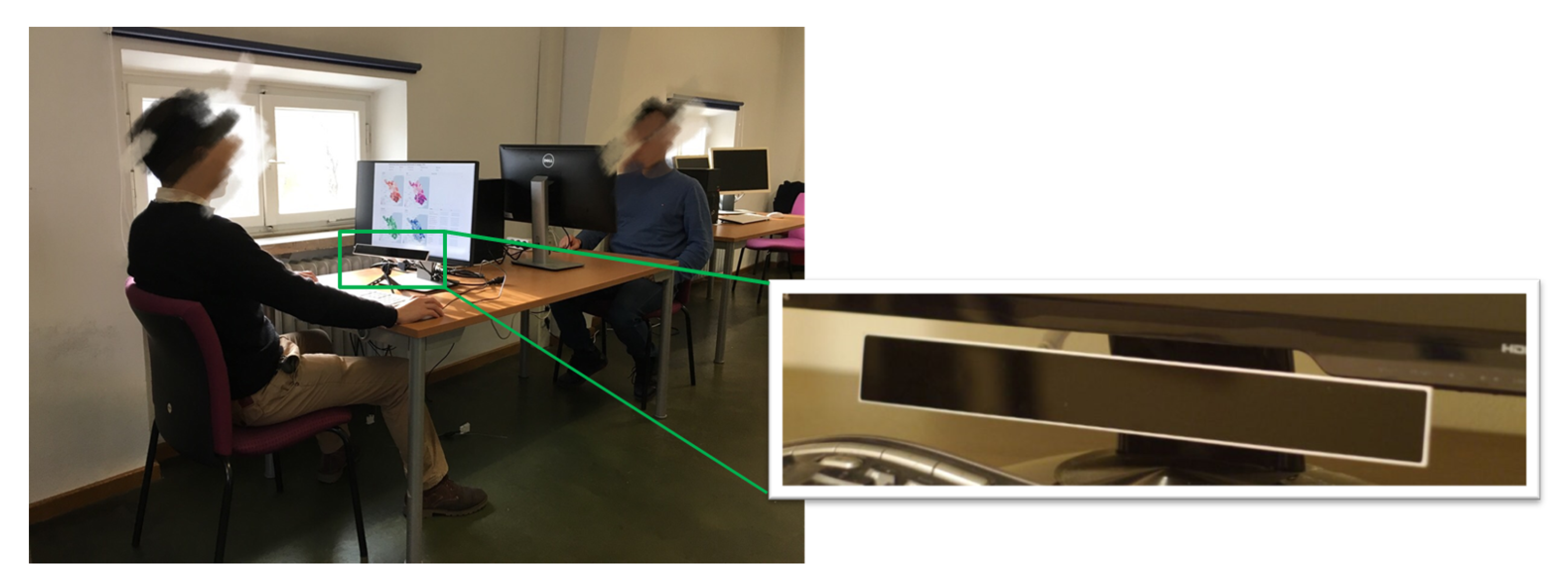
Figure 4.
The integrated experiment tool with the step guides. The screenshot shows when the “Start free exploration” item is clicked. On the right side, it shows an example of the items being clicked.
Figure 4.
The integrated experiment tool with the step guides. The screenshot shows when the “Start free exploration” item is clicked. On the right side, it shows an example of the items being clicked.
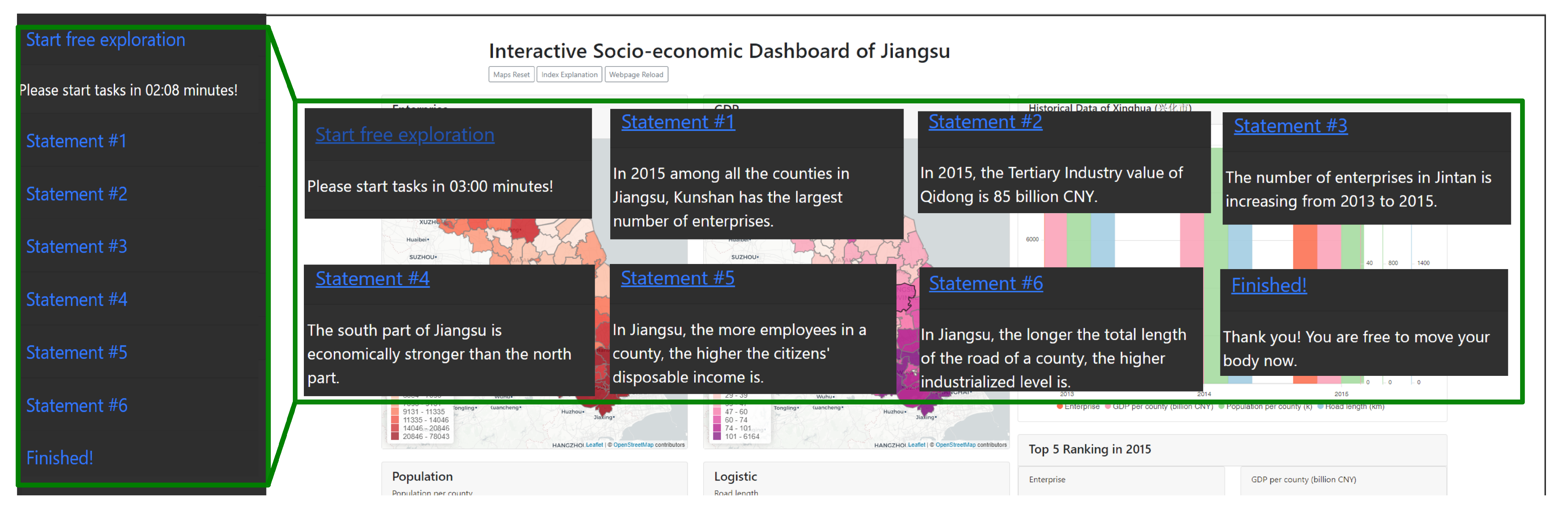
Figure 5.
The outline of the AOIs (a) and the color coding of each AOI (b).

Figure 6.
The heatmaps of all the participants’ fixations during at free exploration stage. The blue dots represents fixations.
Figure 6.
The heatmaps of all the participants’ fixations during at free exploration stage. The blue dots represents fixations.

Figure 7.
The bar charts of the success rates. (a) The success rates of the tasks in increasing difficulties of perception. (b) The success rates across their position in the task sequence.
Figure 7.
The bar charts of the success rates. (a) The success rates of the tasks in increasing difficulties of perception. (b) The success rates across their position in the task sequence.

Figure 8.
The bar charts of the success rates of each task across the position in the task sequence.
Figure 8.
The bar charts of the success rates of each task across the position in the task sequence.

Figure 9.
The boxplots of the response time. (a) The response time of the tasks in increasing difficulties of perception. (b) The response time across their position in the task sequence.
Figure 9.
The boxplots of the response time. (a) The response time of the tasks in increasing difficulties of perception. (b) The response time across their position in the task sequence.

Figure 10.
The boxplots of the response time of each task across the position in the task sequence.

Figure 11.
The response time of the tasks. Failed tasks (red), and the successful tasks (green) in the increasing difficulty levels of perception.
Figure 11.
The response time of the tasks. Failed tasks (red), and the successful tasks (green) in the increasing difficulty levels of perception.
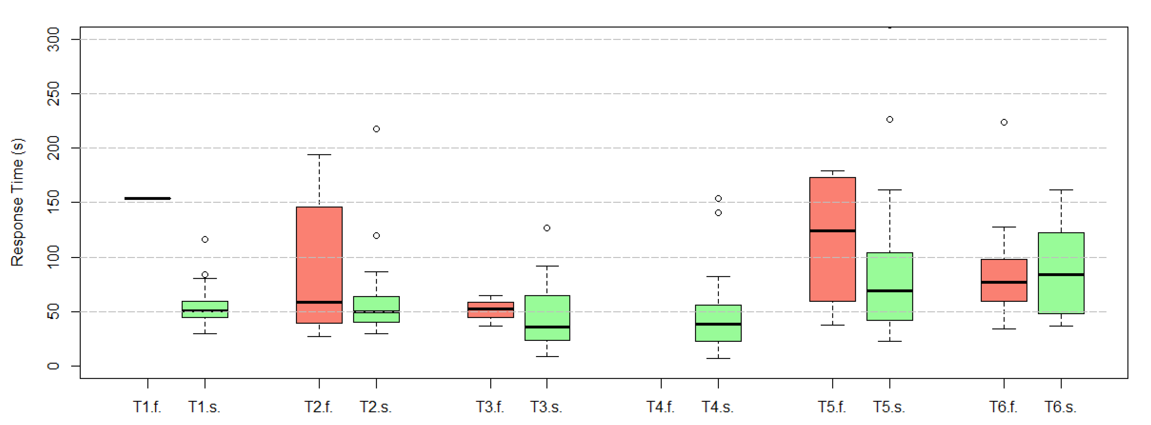
Figure 12.
The visualization of search strategies of T1: (a) The fixation sequence chart. (b) The dwell and transition chart of the successful group. (c) The dwell and transition chart of the failed group. (d) The legend of the AOIs.
Figure 12.
The visualization of search strategies of T1: (a) The fixation sequence chart. (b) The dwell and transition chart of the successful group. (c) The dwell and transition chart of the failed group. (d) The legend of the AOIs.

Figure 13.
The visualization of search strategies of T2: (a) The fixation sequence chart. (b) The dwell and transition chart of the successful group. (c) The dwell and transition chart of the failed group. (d) The legend of the AOIs.
Figure 13.
The visualization of search strategies of T2: (a) The fixation sequence chart. (b) The dwell and transition chart of the successful group. (c) The dwell and transition chart of the failed group. (d) The legend of the AOIs.
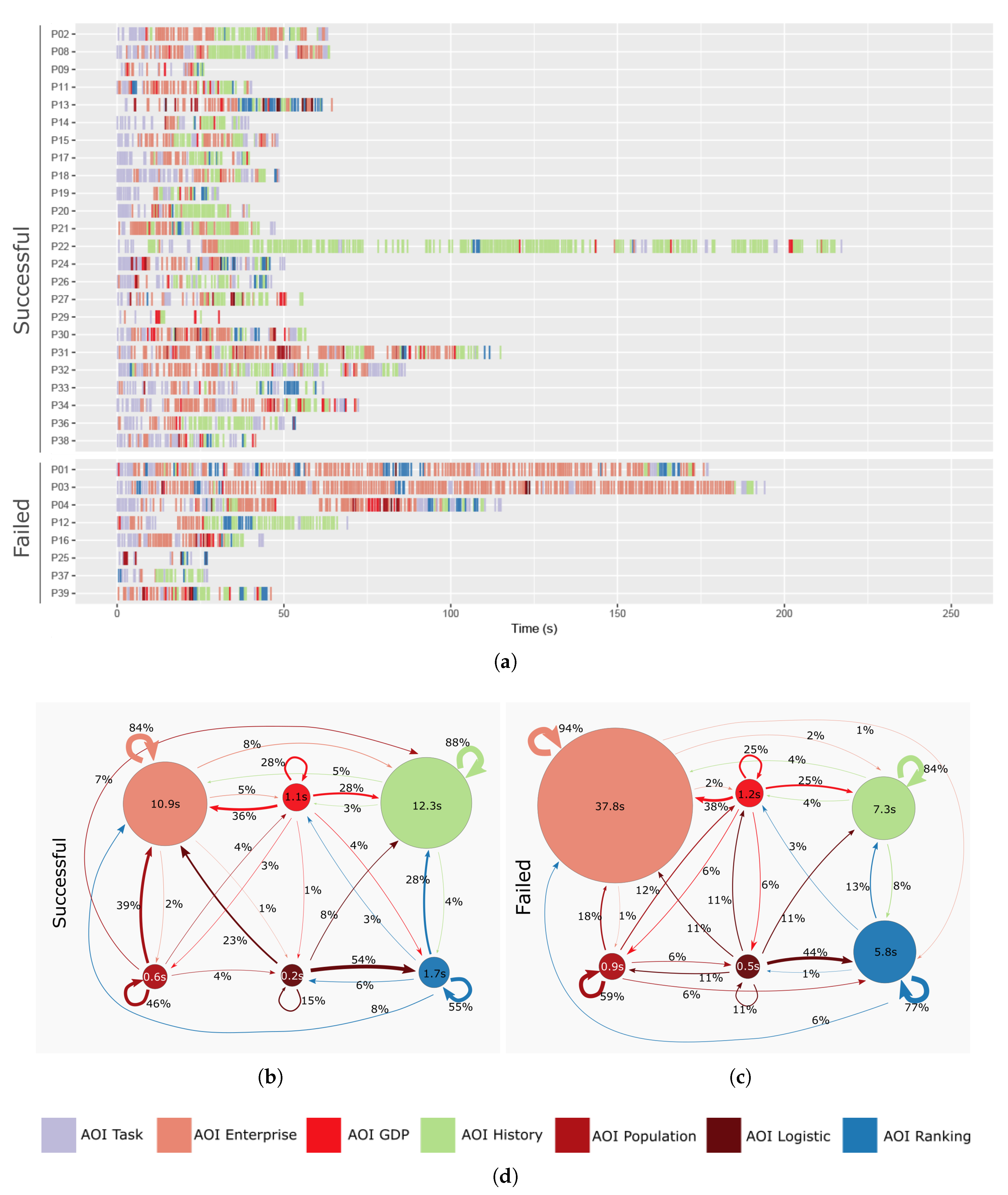
Figure 14.
The visualization of search strategies of T3: (a) The fixation sequence chart. (b) The dwell and transition chart of the successful group. (c) The dwell and transition chart of the failed group. (d) The legend of the AOIs.
Figure 14.
The visualization of search strategies of T3: (a) The fixation sequence chart. (b) The dwell and transition chart of the successful group. (c) The dwell and transition chart of the failed group. (d) The legend of the AOIs.
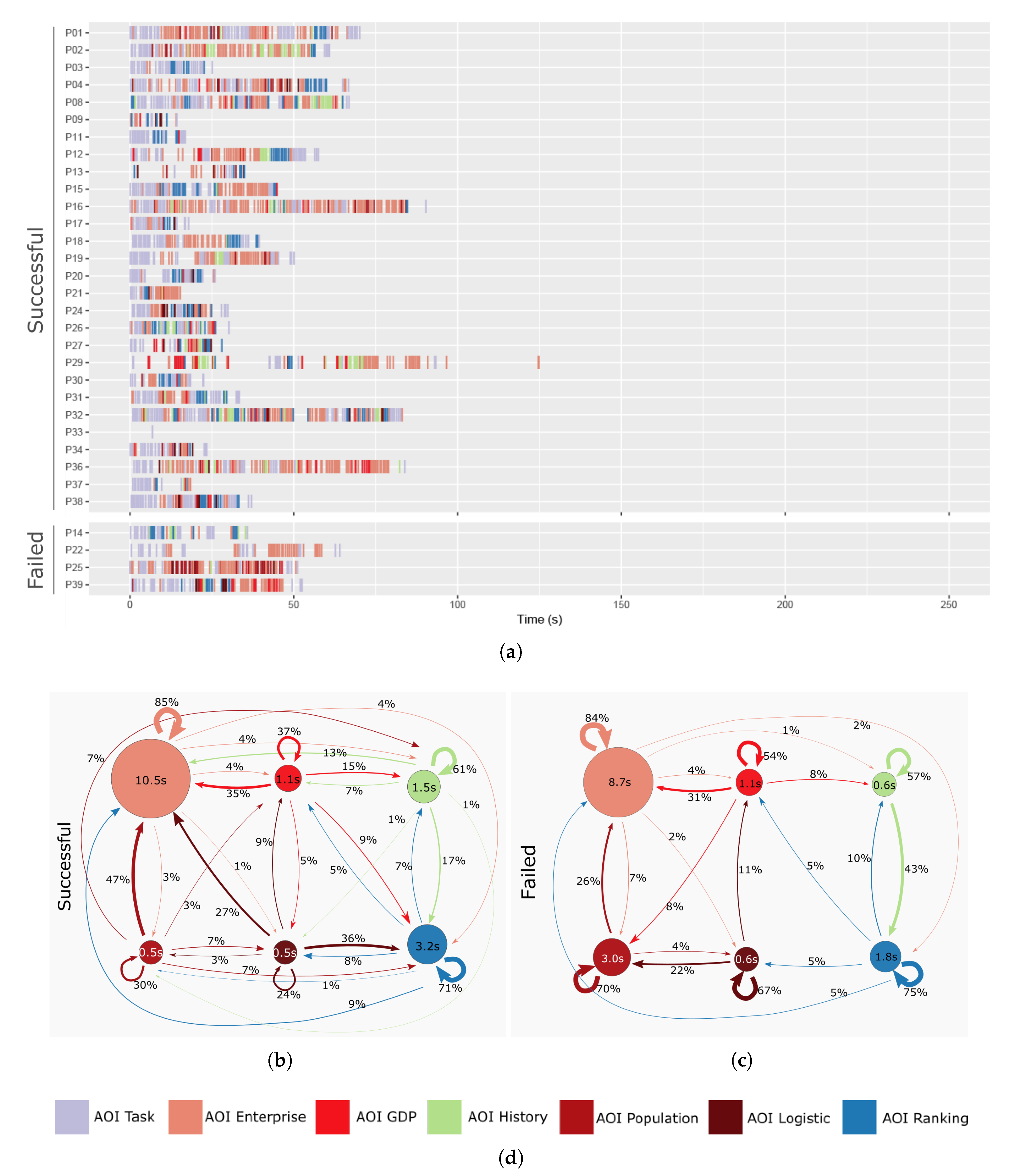
Figure 15.
The visualization of search strategies of T4: (a) The fixation sequence chart. (b) The dwell and transition chart of the successful group. (c) The dwell and transition chart of the failed group. (d) The legend of the AOIs.
Figure 15.
The visualization of search strategies of T4: (a) The fixation sequence chart. (b) The dwell and transition chart of the successful group. (c) The dwell and transition chart of the failed group. (d) The legend of the AOIs.

Figure 16.
The visualization of search strategies of T5: (a) The fixation sequence chart. (b) The dwell and transition chart of the successful group. (c) The dwell and transition chart of the failed group. (d) The legend of the AOIs.
Figure 16.
The visualization of search strategies of T5: (a) The fixation sequence chart. (b) The dwell and transition chart of the successful group. (c) The dwell and transition chart of the failed group. (d) The legend of the AOIs.

Figure 17.
The visualization of search strategies of T6: (a) The fixation sequence chart. (b) The dwell and transition chart of the successful group. (c) The dwell and transition chart of the failed group. (d) The legend of the AOIs.
Figure 17.
The visualization of search strategies of T6: (a) The fixation sequence chart. (b) The dwell and transition chart of the successful group. (c) The dwell and transition chart of the failed group. (d) The legend of the AOIs.

Table 1.
The six statements and their associated answers of the benchmark tasks.
| Task Number | Statement | Answer |
|---|---|---|
| Task 1 | In 2015, the Tertiary Industry value of Qidong is 85 billion Chinese Yuan (CNY). | Wrong |
| Task 2 | The number of enterprises in Jintan increases from 2013 to 2015. | Unkown |
| Task 3 | In 2015, among all the counties in Jiangsu, Kunshan has the largest number of enterprises. | Correct |
| Task 4 | The south part of Jiangsu is economically stronger than the north part. | Correct |
| Task 5 | In Jiangsu, the more employees in a county, the higher the citizens’ disposable income is. | Wrong |
| Task 6 | In Jiangsu, the longer the total length of the road of a county, the higher the industrialized level is. | Wrong |
Table 2.
Benchmark tasks for the evaluation the map-based dashboard.
| Tasks | T1 | T2 | T3 | T4 | T5 | T6 |
|---|---|---|---|---|---|---|
| Description | Find an attribute of a place. | Find the attribute temporal trend of a place. | Identify a place with the highest attribute value. | Summarize the spatial distribution of an attribute. | Compare the spatial distribution of two attributes. | Abstract the attributes. |
| Compare the spatial | ||||||
| distribution of two attributes. | ||||||
| Search Area | Single | Single | Multiple | Multiple | Multiple | Multiple |
| Search Time | Single | Multiple | Single | Single | Single | Single |
| Search Attribute | Single | Single | Single | Single | Multiple | Multiple |
| Query type | State | Change | Order | State | State | State |
| Cognitive Operation | Identification | Comparison | Identification, Comparison | Comparison, Summary | Comparison, Summary | Comparison, Summary, Deduction |
| Dashboard Interaction | Query, Switch content | Query, Highlight * | Switch content * | Switch content * | Switch content | Switch content * |
| Data Availability | High | High | High | High | High | Middle |
* Owning to the default layer setting, the interactions are optional.
Table 3.
The selected eye movement metrics.
| Metric | Description |
|---|---|
| Sequence | The order of fixation within the AOIs. |
| Dwell time | The sum of all the fixations and saccades within an AOI. |
| Transition | The movement from one AOI to another. |
| Return | It is a transition to an AOI itself, also known as revisit. |
| Transition probability | The probability of the fixation moving from one AOI to another AOI in a sequence. |
Table 4.
The task success rate (%) of each task in different groups.
| Category | Group | Number of Participants | T1 | T2 | T3 | T4 | T5 | T6 | Overall |
|---|---|---|---|---|---|---|---|---|---|
| Overall | Overall | 32 | 96.9 | 75.0 | 87.5 | 100.0 | 87.5 | 62.5 | 84.9 |
| Gender | Female | 17 | 94.1 | 64.7 | 94.1 | 100.0 | 94.1 | 58.8 | 84.3 |
| Male | 15 | 100.0 | 86.7 | 80.0 | 100.0 | 80.0 | 66.7 | 85.6 | |
| Education | Master | 14 | 92.9 | 64.3 | 85.7 | 100.0 | 85.7 | 78.6 | 84.5 |
| Bachelor | 17 | 100.0 | 82.4 | 94.1 | 100.0 | 88.2 | 52.9 | 86.3 | |
| High School | 1 | 100.0 | 100.0 | 0.0 | 100.0 | 100.0 | 0.0 | 66.7 | |
| Previous | Used > 5 times | 12 | 100.0 | 83.3 | 91.7 | 100.0 | 83.3 | 75.0 | 88.9 |
| Dashboard | Used ≤ 5 times | 5 | 100.0 | 60.0 | 80.0 | 100.0 | 60.0 | 40.0 | 73.3 |
| Usage | Heard only | 8 | 100.0 | 87.5 | 87.5 | 100.0 | 100.0 | 50.0 | 87.5 |
| Experience | Never heard | 7 | 85.7 | 57.1 | 85.7 | 100.0 | 100.0 | 71.4 | 83.3 |
Table 5.
The median response time (s) of tasks in different groups.
| Category | Group | Number of Participants | T1 | T2 | T3 | T4 | T5 | T6 | Overall |
|---|---|---|---|---|---|---|---|---|---|
| Overall | Overall | 32 | 37.7 | 51.2 | 49.8 | 38.3 | 70.0 | 78.8 | 357.6 |
| Gender | Female | 17 | 40.1 | 52.6 | 56.9 | 32.3 | 53.8 | 87.3 | 348.4 |
| Male | 15 | 36.7 | 49.4 | 47.9 | 43.1 | 81.9 | 74.8 | 377.4 | |
| Education | Master | 14 | 37.7 | 49.1 | 48.8 | 48.7 | 89.2 | 88.7 | 386.0 |
| Bechalor | 17 | 36.7 | 52.6 | 50.3 | 25.1 | 53.8 | 75.6 | 339.7 | |
| High School | 1 | 64.3 | 41.7 | 217.8 | 32.9 | 91.4 | 48.7 | 496.8 | |
| Previous | Used > 5 times | 12 | 32.2 | 52.8 | 59.5 | 38.0 | 86.2 | 74.2 | 388.3 |
| Dashboard | Used ≤ 5 times | 5 | 40.1 | 45.2 | 43.9 | 56.0 | 96.5 | 97.9 | 445.9 |
| Usage | Heard only | 8 | 31.6 | 50.7 | 44.0 | 33.3 | 67.3 | 94.3 | 315.1 |
| Experience | Never heard | 7 | 53.0 | 51.4 | 63.2 | 46.7 | 57.8 | 75.6 | 348.4 |
Table 6.
Grouped positive items mentioned by the participants in the interview.
| Group | Item | Frequency |
|---|---|---|
| Views | The spatial panel is helpful | 9 |
| The temporal panel is helpful | 6 | |
| The ranking panel is helpful | 2 | |
| Layout | The color scheme helped in organizing information | 13 |
| The grouped layers helped in factor finding | 4 | |
| The juxtaposition benefits for comparison | 3 | |
| The structured design gives a good overview | 2 | |
| Interaction | The search function is useful in finding places | 15 |
| The interactions of the temporal panel helped them find data quickly | 6 | |
| Mouse hovering and clicking are helpful | 5 | |
| Layer switching is efficient | 2 | |
| Other | Natural to use | 1 |
Table 7.
Grouped negative items mentioned by the participants in the interview.
| Group | Item | Frequency |
|---|---|---|
| Penal | The top margin of the the bars in the temporal panel is sometimes too narrow | 5 |
| The maps shift when the mouse moves close to their boundaries | 5 | |
| The temporal panel is too informative | 3 | |
| The legend intervals are confusing | 3 | |
| The axises in the temporal panel change their ranges | 1 | |
| The axises in the temporal panel are not necessary | 1 | |
| The temporal panel should be split into four charts as other panels | 1 | |
| Mark the important places in the spatial panel | 1 | |
| Layout | Hard to compare two layers in one map | 3 |
| The color scheme is not good for color-blind people | 3 | |
| Only one map in the spatial panel is preferred | 2 | |
| The color hue should be increased in the temporal panel and ranking panel | 2 | |
| The color of the unavailable data should be lighter | 1 | |
| Interaction | The search bar should be in each map / outside the spatial panel | 5 |
| The ranking panel should be clickable | 4 | |
| The selected place should be highlighted on all the maps | 2 | |
| The map legends should be clickable | 2 | |
| Other | The font size is too small | 5 |
| The unavailable data increases the difficulty | 3 | |
| No idea where to look at on the dashboard | 2 | |
| The dashboard is too informative | 2 | |
| The listing of top five municipalities is not interested to the participant | 1 | |
| A learning time is required | 1 | |
| Lack of the economic background information | 1 |
Publisher’s Note: MDPI stays neutral with regard to jurisdictional claims in published maps and institutional affiliations. |
© 2020 by the authors. Licensee MDPI, Basel, Switzerland. This article is an open access article distributed under the terms and conditions of the Creative Commons Attribution (CC BY) license (http://creativecommons.org/licenses/by/4.0/).
Share and Cite
MDPI and ACS Style
Zuo, C.; Ding, L.; Meng, L. A Feasibility Study of Map-Based Dashboard for Spatiotemporal Knowledge Acquisition and Analysis. ISPRS Int. J. Geo-Inf. 2020, 9, 636. https://0-doi-org.brum.beds.ac.uk/10.3390/ijgi9110636
AMA Style
Zuo C, Ding L, Meng L. A Feasibility Study of Map-Based Dashboard for Spatiotemporal Knowledge Acquisition and Analysis. ISPRS International Journal of Geo-Information. 2020; 9(11):636. https://0-doi-org.brum.beds.ac.uk/10.3390/ijgi9110636
Chicago/Turabian StyleZuo, Chenyu, Linfang Ding, and Liqiu Meng. 2020. "A Feasibility Study of Map-Based Dashboard for Spatiotemporal Knowledge Acquisition and Analysis" ISPRS International Journal of Geo-Information 9, no. 11: 636. https://0-doi-org.brum.beds.ac.uk/10.3390/ijgi9110636
Note that from the first issue of 2016, this journal uses article numbers instead of page numbers. See further details here.