A New Algorithm for Calculating the Flow Path Curvature (C) from the Square-Grid Digital Elevation Model (DEM)

Abstract

This paper proposes a flow-path-network-based (FPN-based) algorithm, constructed from a square-grid digital elevation model (DEM) to improve the simulation of the flow path curvature (C). First, the flow-path network model was utilized to obtain an FPN. Then, a flow-path-network-flow-path-curvature (FPN-C) algorithm was proposed to estimate C from the FPN. The experiments consisted of two sections: (1) quantitatively evaluating the accuracy using 5 m DEMs generated from the mathematical ellipsoid and Gauss models, and (2) qualitatively assessing the accuracy using a 30 m DEM of a real-world complex region. The three algorithms proposed by Evans (1980), Zevenbergen and Throne (1987), and Shary (1995) were used to validate the accuracy of the new algorithm. The results demonstrate that the C value of the proposed algorithm was generally closer to the theoretical C value derived from two mathematical surfaces. The root mean standard error (RMSE) and mean absolute error (MAE) of the new method are 0.0014 and 0.0002 m, reduced by 42% and 82% of that of the third algorithm on the ellipsoid surface, respectively. The RMSE and MAE of the presented method are 0.0043 and 0.0025 m at best, reduced by up to 35% and 14% of that of the former two algorithms on the Gauss surface, respectively. The proposed algorithm generally produces better spatial distributions of C on different terrain surfaces.

1. Introduction

Terrain curvature is an important topographic parameter that reflects the shape characteristics and concave–convex change in different orientations [1,2], and effects the distribution of the soil organic content [3,4]. It has significant application values in terrain analysis [5,6,7,8,9], hydrology [10,11,12,13], soil [14,15,16,17], hazard [18,19,20], and other fields [21,22,23]. The curvature is related to the orientation and has different definitions of geometry and geology [24].

For a long time, a variety of curvatures developed by researchers have been used to meet the requirements of practical applications [25,26,27,28,29,30], such as the mean curvature, maximum curvature, minimum curvature, plan curvature, profile curvature, tangential curvature, flow path curvature, and so on. Less acknowledged is the flow path curvature (C), which is also known as the rotor curvature or streamline curvature [31]. It measures the rate of the change of the flow paths along the horizontal direction, and describes the degree of twisting of the flow lines [4,32,33,34]. Although the flow path curvature was not considered in the complete classification system of curvatures constructed by Shary [35] at first, it has been widely utilized in the theory of the electromagnetic field [36]. For example, Pradhan and Guha [37] discussed the effects of the flow path curvature on the downstream evolution of the three-dimensional flow field to accurately make the corrections of the field in the bifurcation model. Results showed that the flow path curvature is mainly responsible for generating the Dean-type secondary circulation and skewed velocity distributions. Pathak, et al. [38] studied the impact of the flow path curvature on the flow field in the k–ε turbulence model and validated the superiority of the improved model with this curvature. Yang and Tucker [39] selected some widely used turbulence models to assess their performance affected by large flow path curvature and demonstrated that the proper corrections of the flow path curvature can reduce the large solution errors. It still has a few applications in other fields. For example, Tjerry and Fredsøe [40] presented that the flow path curvature is another control factor of the geometry of a fully developed sand wave and certified that this curvature is necessary to determine the position of the maximum sediment transport under low riverbed shear stresses. Bagheri and Kabiri-Samani [41] researched the simulation of the flow over the streamlined weirs based on numerical modeling and proved that a proper curvature of the streamlines can reduce the adverse flow situations and generate a favorable weir structure along the channels. Foroutan, et al. [42] conducted the unsupervised classification of an arid mountainous area based on twenty-two digital elevation model (DEM) derivatives including the flow path curvature. Results demonstrated that this classification is conducive to the uniform division of the area and identification of debris, gravity, and wash slopes. Moreover, it may be beneficial to perform surface runoff simulation due to its impact on the flow velocity of water and surface sediment [3], which will be the topic of our next research. The accuracy and reliability of flow path curvature are still worth exploring. Thus, in this paper, we consider this type of curvature in more detail.

The terrain surface can be described solely by a continuous and single-valued representation $z=f\left(x,y\right)$ and here, $x$ and $y,$ respectively, indicate the coordinates in the $x$ direction and $y$ direction, and $z$ is the elevation. The flow path curvature is estimated by the first-order ($f_x$ and $f_y$) and second-order partial derivatives ($f_{xx}$, $f_{xy}$ and $f_{yy}$). It can be defined as $(\left(f_x{}^2-f_y{}^2\right)\ast f_{xy}-f_x\ast f_y\ast (f_{xx}-f_{yy})/{\left(f_x{}^2+f_y{}^2\right)}^{3/2}$ (units: m⁻¹) by Shary [26]. It is measuring the twist of flow lines. When it is larger than zero, flow lines rotate clockwise. When it is smaller than zero, flow lines rotate counterclockwise, otherwise the flow line does not swing along the straight line [3,42,43]. The flow path curvature is often derived from the square-grid digital elevation model (DEM), which is valued for its simple structure and continuity in the representation of topographic surfaces.

The commonly-used algorithms use the center grid cell and its eight surrounding grid cells based on a moving window of 3 × 3 to calculate the C of the center grid cell. The elevation value of the nine grid cells is approximated by the differentiate operation or local fitting curve. For example, the method proposed by Evans [44] uses the six-parameter second-order polynomial to represent the terrain surface, and derives different partial derivatives by the least-squares fitting algorithm to calculate C. It has a high accuracy when considering the smoothing of the high-frequency noise of the DEM [24,45]. Under the above method, Zevenbergen and Thorne [46] proposed a method which utilizes the partial nine-parameter fourth-order polynomial to describe the surface, and so the fitting curve can be passed through the nine grid cells and obtain the solely different partial derivatives for the C calculation. Its aim was to enhance the accuracy of the different partial derivatives, but it has not achieved the desired results because it lacks the smoothing and denoising effect of DEM [43]. The high-order polynomial interpolation method may result in incorrect topographic features [24].

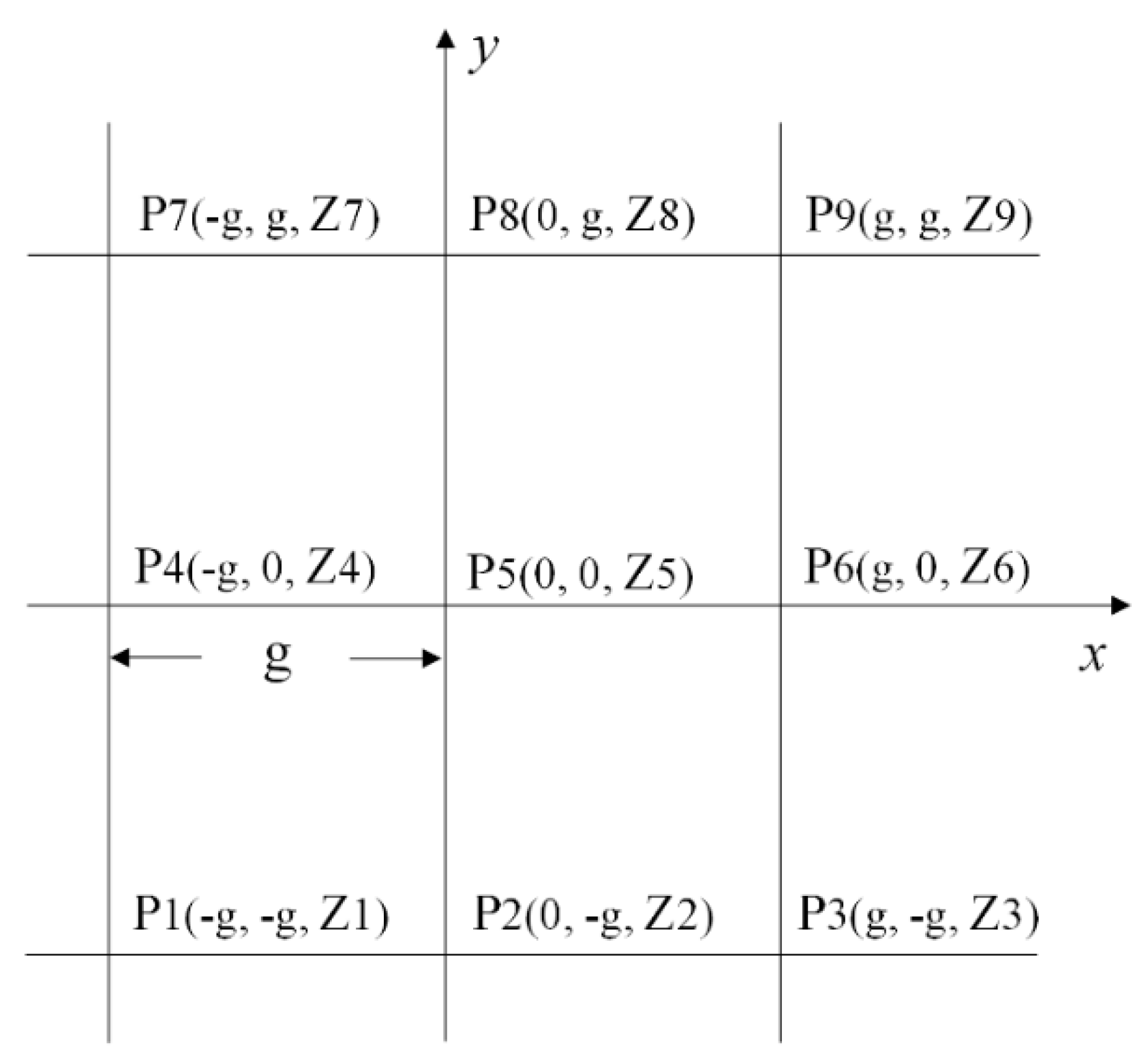
Because the general second-order surface does not pass through all of the nine grid cells, the method presented by Shary [35] employs the constrained five-parameter second-order polynomial to fit the surface, and is also based on the least-squares fitting algorithm to derive the different partial derivatives for estimating C. It is similar to the Evans algorithm, except for the different averaging processes. Considering the equidistant distribution characteristics of a regular grid, Moore, et al. [47] proposed a difference method using the numerical differentiation to calculate partial derivatives for the C estimation. It directly uses the elevation of the center grid cell and eight neighboring grid cells to derive the different partial derivatives for estimating C. It is similar to the algorithm proposed by Zevenbergen and Thorne [46], but they calculated the second-order partial derivatives using different methods. In order to improve accuracy and adaptability to the different terrain surfaces, Shary, Sharaya and Mitusov [30] proposed the modified Evans–Young method, which is based on the Evans algorithm, to calculate the curvature after using filters to handle the center grid cell. The above mentioned methods utilize the local terrain surface representation to derive the partial derivatives by the different interpolation algorithm and a moving window. They are more helpful to consistently extract the local curvature, but are not suitable for complex topography regions for higher-scale problems in terrain analysis [48]. Moreover, the accuracy of these algorithms is affected by interpolation errors, and there are difficulties in selecting suitable algorithms for the applications.

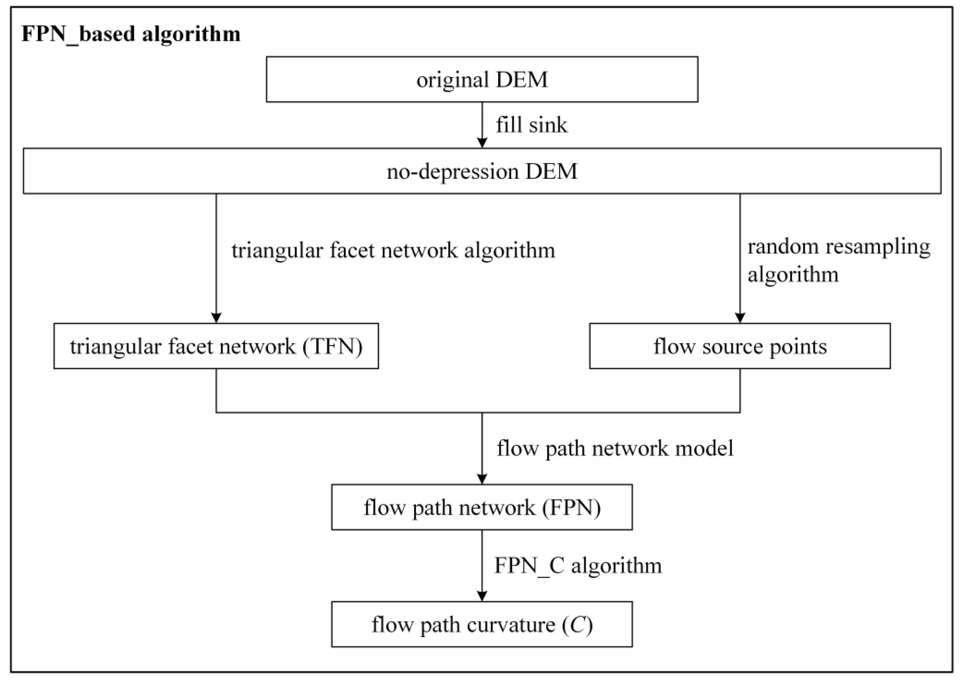
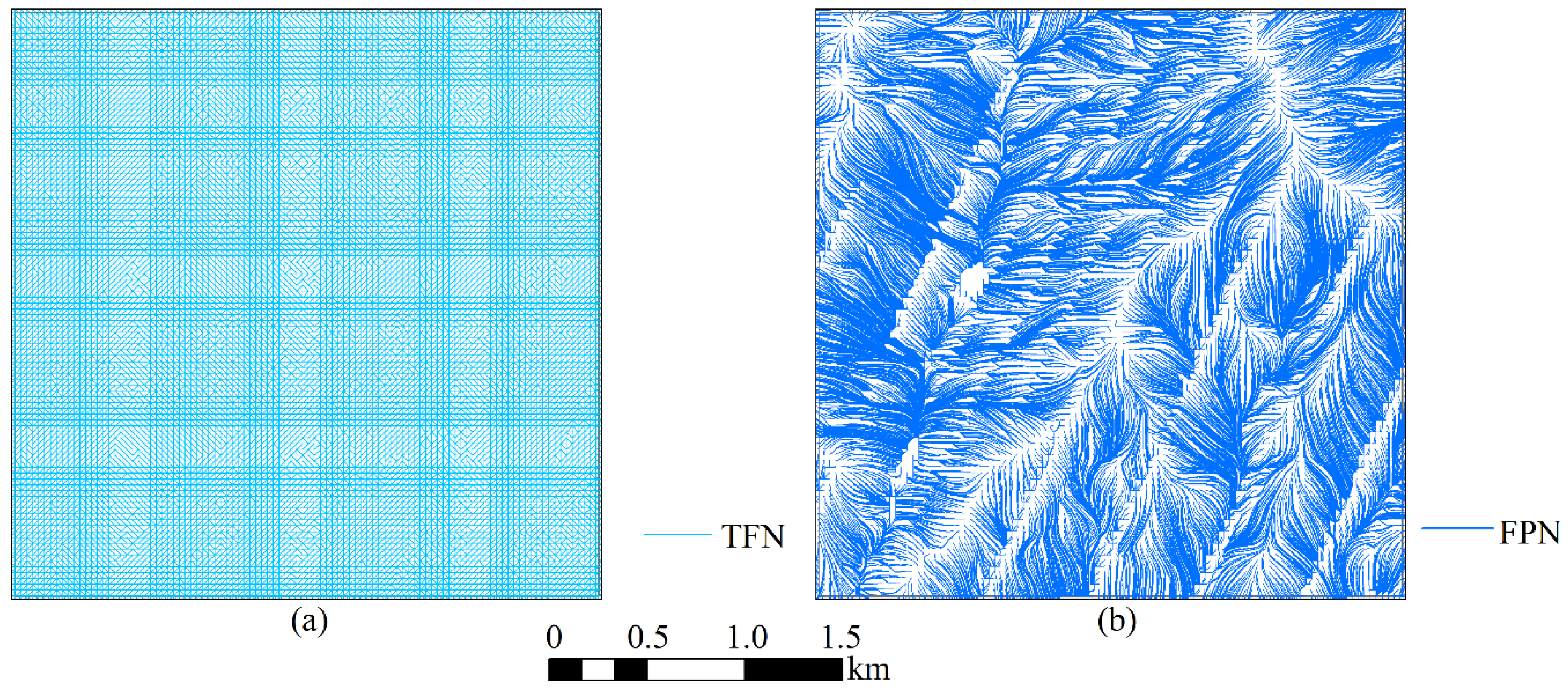
To overcome the aforementioned disadvantages, we present a flow-path-network-based (FPN-based) algorithm to derive the flow path curvature (C) based on the vector-based approach. It uses the flow-path network model [49] to generate the one-dimensional flow path network (FPN). Then, a new flow-path-network-flow-path-curvature (FPN-C) algorithm is presented to calculate the C from the FPN. It aims to improve the calculation accuracy of the C and avoid the interpolation error and the choice of the calculation algorithm in practical applications. The experiments consisted of two sections: (1) quantitatively evaluating the accuracy of the new algorithm on the 5 m DEMs generated from the mathematical ellipsoid and Gauss surface models, and (2) qualitatively assessing the accuracy of the proposed method by using a real-world DEM of a hilly plateau and mountainous region.

The structure of the paper is arranged as follows. The methods of the FPN-based approach are presented in Section 2. Section 3 describes the experiments. The experiment results are shown in Section 4. The accuracy of the proposed approach is discussed in Section 5. Section 6 concludes the paper and illustrates directions for further research.

2. Methods

The methods consist of two sections in this paper: (1) obtaining a flow path network (FPN) using the flow-path network model; (2) proposing an FPN-C algorithm to calculate the flow path curvature (C) from the FPN. The detailed process of the FPN-based algorithm is shown in Figure 1.

2.1. Obtaining a Flow Path Network (FPN) Using the Flow-Path Network Model

In this paper, the flow path network (FPN) is tracked by the flow-path network model [49], and its detailed steps are shown in Figure 1. First, a no-depression DEM was acquired by filling the sinks and local pits of the original DEM. Second, the triangular facet network algorithm [50] was used to construct the triangular facet network (TFN). Third, the flow direction of the triangular facets over the TFN was determined by its aspect and slope as shown in Figure 2, which were calculated by the equations presented by Zhou, Pilesjö and Chen [50]. When the coordinate values of the three vertices of a triangular facet were assumed as $p_1\left(x_1,y_1,z_1\right)$, $p_2\left(x_2,y_2,z_2\right),$ and $p_3\left(x_3,y_3,z_3\right)$, the plane equation of the facet could be specified as $z=a\ast x+b\ast y+c$. Here, $a$, $b,$ and $c$ could be derived from Equation (1). The aspect ($\alpha$) and slope ($\beta$) could be derived from Equation (2). Thus, the flow direction over the triangular facet could be represented by a vector whose direction and length were determined by the aspect and slope, respectively. The process of estimating the flow direction was different from that of Terrain Analysis Using Digital Elevation Models (TauDEM). This is because the latter utilizes the multiple flow direction (D∞) algorithm to estimate the flow direction which is represented as the direction of the steepest downward slope over the eight triangular facets centered on a grid cell [51]. The downward slope of each triangular facet is symbolized by a vector whose direction and length are determined by the ratio of elevation change to length in the $x$ direction and $y$ direction, respectively [52]. It obtained the flow direction using grid-based DEM, and the method in this paper estimated the flow direction based on the three-dimensional vector facet. Fourth, the random resampling algorithm [53] was used to obtain the flow source points from the original DEM. Finally, combining the flow direction of the triangular facets over the TFN with the flow source points, an FPN was tracked based on the flow-path network model; its detailed steps have already been described in this paper [49].

$$\{\begin{array}{c}a=\frac{\left(y_1 - y_3\right) \ast \left(z_1 - z_2\right) - \left(y_1 - y_2\right) \ast \left(z_1 - z_3\right)}{\left(x_1 - x_2\right) \ast \left(y_1 - y_3\right) - \left(x_1 - x_3\right) \ast \left(y_1 - y_2\right)}\\ b=\frac{\left(x_1 - x_2\right) \ast \left(z_1 - z_2\right) - \left(x_1 - x_3\right) \ast \left(z_1 - z_{2s}\right)}{\left(x_1 - x_2\right) \ast \left(y_1 - y_3\right) - \left(x_1 - x_3\right) \ast \left(y_1 - y_2\right)}\\ c=z_1 - a \ast x_1 - b \ast y_1\end{array}$$

(1)

$$\{\begin{array}{c}\alpha ={\tan }^{-1}\left(\sqrt{a^2+b^2}\right)\\ \beta =\pi -{\tan }^{-1}\left(\frac{b}{a}\right)+\frac{\pi }{2}\ast \frac{a}{\left|a\right|}\end{array}$$

(2)

2.2. Proposing an FPN-C Algorithm to Calculate the Flow Path Curvature (C) from the FPN

Considering the relatively stable curvature of the one-dimensional flow line over the FPN, an FPN-C algorithm was proposed to calculate the flow path curvature (C) from the flow line. The algorithm directly estimated the C based on the vector flow line rather than the first-order and second-order derivations of the scattered grid cells.

2.2.1. Selecting the Suitable Flow Line to Calculate the Flow Path Curvature (C)

The flow path curvature (C) of a grid cell was assumed to be derived from the flow line passing the grid cell. There may be numerous flow lines through a grid cell, and they are parallel for the same flow direction of each grid cell. Therefore, it was necessary to select the suitable flow line from the FPN.

The selection method is as follows: (1) Judge whether the number of flow lines passing through the calculated grid cell is equal to 1. If it is equal to 1, there will be only one flow line passing through the grid cell, and the flow line will be regarded as the suitable flow line, otherwise; (2) find all of the flow lines passing through the calculated grid cell, namely, the pass-lines; (3) select the flow lines throughout the calculated grid cell from the pass-lines, namely, the through-lines. The standard throughout a grid cell depends on the length of the flow line within the grid cell and whether it is larger than the length of the grid cell; (4) regard the longest line among the through-lines as the suitable flow line.

2.2.2. Smoothing the Flow Line by the B-Spline Interpolation Method

The most suitable flow line within a grid cell consists of several break points; each broken line may have significantly different curvature, and it is not reasonable to expect that any of the broken lines can be utilized to estimate C. Thus, we smoothed the flow line so that the whole line in a grid cell could be used to derive an accurate flow path curvature (C).

The spline interpolation method is commonly used to obtain smooth curves in the mathematical [54,55,56], physical [57,58,59,60], and other fields [61,62,63,64]. In this study, the flow line was smoothed by the B-spine interpolation method (B-spline method), which is suitable for handling the multivalued functions that may appear on the flow line. To keep the overall smoothness and a continuous slope and curvature at the break points, the cubic B-spine interpolation algorithm was utilized to smooth the flow line by using these break points within the calculated grid cell. Moreover, the flow line was cut up by a threshold to reduce the likelihood of overfitting. To prevent the lines in the grid cell being too short and the number of the break points not being enough, the threshold should not be too small.

According to the principle of the cubic B-spline interpolation algorithm, we could obtain a B-spline curve ($P\left(u\right)$), which is a piecewise function, as shown in Equation (3). If there were $n+1$ points and a node vector ($U=\left\{u_0,u_1,\dots ,u_{n+k+1}\right\}$, $(k=3$)) used to smooth the curve, there would be an $n$ basic function. Each function ($N_{i,k}\left(x\right)$, $\left(i=0,1,\dots ,n\right)$) could be defined as Equation (4), and the operational relationship between the basic functions is shown in Figure 3. Under the rules of interpolation continuity and differential continuity, we could obtain Equation (5). Combing the equation with Equations (3) and (4), we could calculate the $P_0$, $P_1$, $P_2$, …, $P_n$ to obtain the $P\left(u\right)$. Figure 4 illustrates a smoothing flow line by the cubic B-spline method.

$$P\left(u\right)=P_0\ast N_{0,3}\left(u\right)+P_1\ast N_{1,3}\left(u\right)+P_2\ast N_{2,3}\left(u\right)+\cdots +P_n\ast N_{n,k}\left(u\right)$$

(3)

$$\{\begin{array}{c}{N}_{i,0}\left(u\right)=\{\begin{array}{c}1,u_i<u<u_{i+1}\\ 0,other\end{array}\\ N_{i,m}\left(u\right)=\frac{\left(u-u_i\right)\ast N_{i,k-1}\left(u\right)}{u_{i+k}-u_i}+\frac{\left(u_{i+k+1}-u\right)\ast N_{i+1,k-1}\left(u\right)}{u_{i+k+1}-u_{i+1}},m\le 3,u_k\le u\le u_{n+1}\end{array}$$

(4)

$${N^{\prime }}_{i,m}\left(u\right)=\frac{k-1}{u_{i+k+1}-u_i}\ast N_{i,m-1}\left(u\right)+\frac{k-1}{u_{i+k}-u_{i+1}}\ast N_{i+1,m-1}\left(u\right)$$

(5)

2.2.3. Fitting the Circle by the Least Square Algorithm

The premise of fitting a circle is selecting a series of points from the smoothing flow line in the calculated grid cell. Therefore, it was key to choose the proper points from the line in the grid cell.

In this paper, the points were obtained by equally dividing the smoothing flow line, such as the black points shown in Figure 5. The least square algorithm with the greatest effect was utilized to fit the circle (the assumption of the circle equation is $x^2+y^2+a\ast x+b\ast y+c=0$) by the several points in the calculated grid cell (the assumptions of these points are $\left(x_i,y_i\right)$, $i=1,2,3,\dots ,n$). Once the value of $a$,$b,$ and $c$ was determined, the circle was obtained. According to the principle of the least square method, we could obtain the objective function (as shown in Equation (6)). The optimal circle was matched when the objective function reached its minimum, and $a$, $b,$ and $c$ could be acquired from Equation (7).

$$f\left(a,b,c\right)={{\displaystyle \sum }}_{i=1}^n{\left(x_i^2+y_i^2+a\ast x_i+b\ast y_i+c\right)}^2$$

(6)

$$\left(\begin{array}{c}{{\displaystyle \sum }}_{i=1}^n{x}_i^3+{{\displaystyle \sum }}_{i=1}^n{x}_i\ast y_i^2\\ {{\displaystyle \sum }}_{i=1}^n{y}_i^3+{{\displaystyle \sum }}_{i=1}^n{x}_i^2\ast y_i\\ {{\displaystyle \sum }}_{i=1}^n{x}_i^2+{{\displaystyle \sum }}_{i=1}^n{y}_i^2\end{array}\right)+\left(\begin{array}{ccc}{{\displaystyle \sum }}_{i=1}^n{x}_i^2& {{\displaystyle \sum }}_{i=1}^n{x}_i\ast y_i& {{\displaystyle \sum }}_{i=1}^n{x}_i\\ {{\displaystyle \sum }}_{i=1}^n{x}_i\ast y_i& {{\displaystyle \sum }}_{i=1}^n{y}_i^2& {{\displaystyle \sum }}_{i=1}^n{y}_i\\ {{\displaystyle \sum }}_{i=1}^n{x}_i& {{\displaystyle \sum }}_{i=1}^n& n\end{array}\right)\left(\begin{array}{c}a\\ b\\ c\end{array}\right)=\left(\begin{array}{c}0\\ 0\\ 0\end{array}\right)$$

(7)

where $f\left(a,b,c\right)$ denotes the objective function, $i$ denotes the $i^{th}$ point, and $x_i\mathrm{and}{y}_i$ are the coordinate values of the $i^{th}$ point in the x direction and y direction, respectively.

The method can use more than three points to complete the circle fitting, and when more points are applied it is possible to achieve a better performance. Thus, the standard of dividing the line evenly in this paper was ensuring that there were more than ten points within the calculated grid cell. The red circle in Figure 5 was acquired by these points in the black grid cell, based on the above algorithm.

2.2.4. Calculating the C by the Fitting Circle

According to Figure 5, the flow path curvature (C) of each grid cell was computed by the radius of the fitting circle (the assumption of the radius is $r$) and any three ordered points (the assumptions of the three blue points are $P_0\left(x_0,y_0\right)$, $P_1\left(x_1,y_1\right)$, $P_2\left(x_2,y_2\right)$) in the grid cell. The circle radius could be derived from three parameters of the circle (assumption of the parameters are a, b, c) by the equation ($r=0.5\ast \sqrt{a^2+b^2-4\ast c}$). Thus, the absolute value of C was the reciprocal of the radius, namely, $1/r$. Its plus–minus sign was determined by the cross product of $\overrightarrow{P_0{P}_1}$ and $\overrightarrow{P_1{P}_2}$. If $\overrightarrow{P_0{P}_1}·\overrightarrow{P_1{P}_2}$ was greater than zero, C would be $-1/r$, which denoted that the counterclockwise flow rotated in the flow direction, otherwise, C would be $1/r$, which denoted that the clockwise flow rotated in the flow direction. In addition, if C was zero, the flow would not have any swing.

3. Experiments

We conducted experiments using two mathematical models to quantitatively evaluate the accuracy of the new algorithm in this study. Moreover, the new algorithm was applied to a real-world DEM of a hilly plateau and mountainous area, located in the central Ganzi Tibetan Autonomous Prefecture of Sichuan Province to qualitatively assess its accuracy.

3.1. Quantitative Experiment

The ellipsoid surface model (Equation (8)) and Gauss surface model (Equation (9)) [65,66] were selected to generate the DEMs with a 5 m resolution. We utilized the DEMs generated from four ellipsoid surface models (namely, E1, E2, E3, and E4) and four Gauss surface models (namely, G1, G2, G3, and G4) with different complexities to validate the accuracy of the new method.

Table 1. Parameters of the eight mathematical surface models.

Surface Types	Parameters
E1	$a=400,b=300,c=300,-400<x<400,-300<y<300$
E2	$a=400,b=300,c=800,-400<x<400,-300<y<300$
E3	$a=400,b=300,c=1200,-400<x<400,-300<y<300$
E4	$a=400,b=300,c=1600,-400<x<400,-300<y<300$
G1	$a=3,b=10,c=1/3,M=500,N=500,-500\le x,y\le 500$
G2	$a=30,b=100,c=3,M=500,N=500,-500\le x,y\le 500$
G3	$a=60,b=200,c=6,M=500,N=500,-500\le x,y\le 500$
G4	$a=90,b=300,c=9,M=500,N=500,-500\le x,y\le 500$

shows the parameters of the eight mathematical surfaces. The theoretical flow path curvature (C) could be derived from the mathematical formulas of the equations summarized in

Table 2. Formulas describing the two mathematical surfaces and calculating the theoretical C value.

Surface Types	Formulas Describing the Surfaces and Calculating Theoretical the Theoretical C Value
Ellipsoid	$f_x=-\frac{c^2\ast x_p}{a^2\ast z_p},f_y=-\frac{c^2\ast y_p}{b^2\ast z_p}$ $f_{xx}=-\frac{c^4\ast \left(1-\frac{y_p^2}{b^2}\right)}{a^2\ast z_p^3},f_{xy}=-\frac{c^4\ast x_p\ast y_p}{a^2\ast b^2\ast z_p^3},f_{yy}=-\frac{c^4\ast \left(1-\frac{x_p^2}{a^2}\right)}{b^2\ast z_p^3}$ $C^1=\left(\left(f_x{}^2-f_y{}^2\right)\ast f_{xy}-f_x\ast f_x\ast \left(f_{xx}-f_{yy}\right)\right)/{\left(f_x{}^2+f_y{}^2\right)}^{3/2}$
Gauss	$p=e^{-{\left(\frac{x}{M}\right)}^2-{\left(\frac{y}{N}+1\right)}^2},q=e^{-{\left(\frac{x}{M}\right)}^2-{\left(\frac{y}{N}\right)}^2},r=e^{-{\left(\frac{x}{M}+1\right)}^2-{\left(\frac{y}{N}\right)}^2}$ $a_1=-\frac{4\ast x_p}{M^2}+\frac{2\ast x_p{}^3}{M^4},a_2=\frac{0.2}{M}-\frac{3.4\ast x_p{}^2}{M^3}+\frac{2\ast x_p{}^4}{M^5}+\frac{2\ast x_p\ast y_p{}^5}{M^2\ast N^5}$ $a_3=-\frac{2\ast x_p}{M^2}+\frac{2}{M},b_1=(1-{\left(\frac{x_p}{M}\right)}^2)\ast (\frac{2\ast y_p}{N^2}+\frac{2}{M}),b_2=\frac{2\ast y_p}{N^2}$ $b_3=\frac{5\ast y_p{}^4}{N^5}+\frac{0.4\ast x_p\ast y_p}{M\ast N^2}-\frac{2\ast x_p{}^3\ast y_p}{M^3\ast N^2}-\frac{2\ast y_p{}^6}{N^7}$ $c_1=\frac{4}{M^2}-\frac{14\ast x_p{}^2}{M^4}+\frac{4\ast x_p{}^4}{M^6},c_2=\frac{2}{M^2}-{\left(\frac{2\ast x_p}{M^2}+\frac{2}{M}\right)}^2$ $c_3=\frac{7.2\ast x_p}{M^3}-\frac{14.8\ast x_p{}^3}{M^5}-\frac{2\ast y_p{}^5}{M^2\ast N^5}+\frac{4\ast x_p{}^5}{M^7}+\frac{4\ast x_p{}^2\ast y_p{}^5}{M^4\ast N^5}$ $d_1=\left(\frac{4\ast x_p}{M^2}-\frac{2\ast x_p{}^3}{M^4}\right)\ast \left(\frac{2\ast y_p}{N^2}+\frac{2}{N}\right),d_2=\left(\frac{2\ast x_p}{M^2}+\frac{2}{M}\right)\ast \frac{2\ast y_p}{N^2}$ $d_3=\frac{10\ast x_p\ast y_p{}^4}{M^2\ast N^5}+\left(\frac{0.2}{M}-\frac{3.4\ast x_p{}^2}{M^3}+\frac{2\ast x_p{}^4}{M^5}+\frac{2\ast x_p\ast y_p{}^5}{M^2\ast N^5}\right)\ast \left(\frac{2\ast y_p}{N^2}\right)$ $h_1=(1-{\left(\frac{x_p}{M}\right)}^2)\ast (-\frac{2}{N^2}+{\left(\frac{2\ast y_p}{N^2}+\frac{2}{N}\right)}^2),h_2=\frac{2}{N^2}-\frac{4\ast y_p{}^2}{N^4}$ $h_3=\frac{20\ast y_p{}^3}{N^5}+\frac{0.4\ast x_p}{M\ast N^2}-\frac{2\ast x_p{}^3}{M^3\ast N^2}-\frac{22\ast y_p{}^5}{N^7}-\frac{0.8\ast x_p\ast y_p{}^2}{M\ast N^4}+\frac{4\ast x_p{}^3\ast y_p{}^2}{M^3\ast N^4}+\frac{4\ast y_p{}^7}{N^9}$ $f_x=a\ast a_1\ast p-b\ast a_2\ast q+c\ast a_3\ast r,f_y=-a\ast b_1\ast p+b\ast b_3\ast q+c\ast b_2\ast r$ $f_{xx}=-a\ast c_1\ast p+b\ast c_3\ast q+c\ast c_2\ast r,f_{xy}=a\ast d_1\ast p-b\ast d_3\ast q-c\ast d_2\ast r$ $f_{yy}=a\ast h_1\ast p+b\ast h_3\ast q+c\ast h_2\ast r$ $C=\left(\left(f_x{}^2-f_y{}^2\right)\ast f_{xy}-f_x\ast f_x\ast \left(f_{xx}-f_{yy}\right)\right)/{\left(f_x{}^2+f_y{}^2\right)}^{3/2}$

¹ Theoretical flow path curvature (C) value at the point ($x_p$, $y_p$, $y_p$).

.

$$\frac{x^2}{a^2}+\frac{y^2}{b^2}+\frac{z^2}{c^2}=1,z>0$$

(8)

$$z=a\left[1-{\left(\frac{x}{M}\right)}^2\right]e^{-{\left(\frac{x}{M}\right)}^2-{\left(\frac{y}{N}+1\right)}^2}-b\left[\frac{0.2\ast x}{M}-{\left(\frac{x}{M}\right)}^3-{\left(\frac{y}{N}\right)}^5\right]e^{-{\left(\frac{x}{M}\right)}^2-{\left(\frac{y}{N}\right)}^2}-c{e}^{-{\left(\frac{x}{M}+1\right)}^2-{\left(\frac{y}{N}\right)}^2}$$

(9)

In this paper, the 5 m DEMs were resampled to obtain 15,031 and 40,000 flow source points at random on the ellipsoid and Gauss surfaces, respectively. The threshold values of 30, 50, 100, and 150 m were used to cut up the flow line over the FPN on the E1 and G1 in the process of choosing the optimal threshold. During the circle fitting by the least square algorithm, we ensured that there were more than ten points within the calculated grid cell. Next, we selected the optimum threshold value to estimate the C value on E2, E3, E4, G2, G3, and G4. Finally, the simulated C value was compared with the theoretical C value by the root mean standard error (RMSE) and mean absolute error (MAE), to validate its accuracy. The RMSE and MAE are expressed as follows:

$$RMSE=\sqrt{{{\displaystyle \sum }}_{i=1}^n{\left(C_i^{\prime }-C_i\right)}^2/n}$$

(10)

$$MAE={{\displaystyle \sum }}_{i=1}^n\left|C_i^{\prime }-C_i\right|/n$$

(11)

where $C_i$ denotes the theoretical value, $C_i^{\prime }$ denotes the simulated value, $n$ denotes the number of grid cells, and $i$ denotes the $i^{th}$ grid cell.

3.2. Comparison Algorithms

In this study, three common published methods were compared to the proposed method. These algorithms used the elevation values of the surrounding cells to compute the C of the central cell using a 3 × 3 window, as shown in Figure 6.

The first is the method proposed by Evans [44]. The expression of the fitting surface and the equation for calculating C are expressed as Equation (12).

$$\{\begin{array}{c}f\left(xy\right)=a{x}^2+b{y}^2+cxy+dx+ey+f\\ f_x=(Z_3+Z_6+Z_9-Z_1-Z_4-Z_7)/(6\ast g)\\ f_y=(Z_7+Z_8+Z_9-Z_1-Z_2-Z_3)/(6\ast g)\\ f_{xx}=(Z_1+Z_3+Z_4+Z_6+Z_7+Z_9-2\ast (Z_2+Z_5+Z_8\left)\right)/(3\ast g^2)\\ f_{xy}=(Z_9+Z_1-Z_7-Z_3)/(4\ast g^2)\\ f_{yy}=(Z_1+Z_2+Z_3+Z_7+Z_8+Z_9-2\ast (Z_4+Z_5+Z_6\left)\right)/(3\ast g^2)\\ C=\left(\left(f_x{}^2-f_y{}^2\right)\ast f_{xy}-f_x\ast f_x\ast \left(f_{xx}-f_{yy}\right)\right)/{\left(f_x{}^2+f_y{}^2\right)}^{3/2}\end{array}$$

(12)

where $Z_i$ denotes the elevation of the $i^{th}$ grid cell.

The second is the method proposed by Zevenbergen and Thorne [46]. The expression of the fitting surface and the equation for calculating C are expressed as Equation (13).

$$\{\begin{array}{c}f\left(xy\right)=a{x}^2{y}^2+b{x}^{2}y+cx{y}^2+d{x}^2+e{y}^2+fxy+gx+hy+i\\ f_x=(Z_6-Z_4)/(2\ast g)\\ f_y=(Z_8-Z_2)/(2\ast g)\\ f_{xx}=\left(\right(Z_4+Z_6)/2.0-Z_5)/g^2\\ f_{xy}=(Z_9+Z_1-Z_7-Z_3)/(4\ast g^2)\\ f_{yy}=\left(\right(Z_1+Z_8/2.0-Z_5)/g^2\\ C=\left(\left(f_x{}^2-f_y{}^2\right)\ast f_{xy}-f_x\ast f_x\ast \left(f_{xx}-f_{yy}\right)\right)/{\left(f_x{}^2+f_y{}^2\right)}^{3/2}\end{array}$$

(13)

where $Z_i$ denotes the elevation of the $i^{th}$ grid cell.

The third is the method proposed by Shary [35]. The functional expression of the fitting surface and the equation for calculating C are expressed as Equation (14).

$$\begin{array}{c}f\left(xy\right)=a{x}^2+b{y}^2+cxy+dx+ey+Z^5\\ f_x=(Z_3+Z_6+Z_9-Z_1-Z_4-Z_7)/(6\ast g)\\ f_y=(Z_7+Z_8+Z_9-Z_1-Z_2-Z_3)/(6\ast g)\\ f_{xx}=(Z_1+Z_3+Z_7+Z_9+3\ast (Z_4+Z_6)-2\ast (Z_2+3\ast Z_5+Z_8\left)\right)/(5\ast g^2)\\ f_{xy}=(Z_9+Z_1-Z_7-Z_3)/(4\ast g^2)\\ f_{yy}=(Z_1+Z_3+Z_7+Z_9+3\ast (Z_2+Z_8)-2\ast (Z_4+3\ast Z_5+Z_6\left)\right)/(5\ast g^2)\\ C=\left(\left(f_x{}^2-f_y{}^2\right)\ast f_{xy}-f_x\ast f_x\ast \left(f_{xx}-f_{yy}\right)\right)/{\left(f_x{}^2+f_y{}^2\right)}^{3/2}\end{array}$$

(14)

where $Z_i$ denotes the elevation of the $i^{th}$ grid cell.

The three above-mentioned algorithms are referred to hereafter as the Evans, Zevenbergen, and Shary algorithms, respectively. C++ was used to implement the Evans, Zevenbergen, and Shary algorithms, and the proposed algorithm was implemented using C++ and Python.

3.3. A Real-World Application

A 30 m resolution DEM of a hilly plateau and mountainous region was selected to qualitatively prove the accuracy of the new algorithm (Figure 7). The test DEM consisted of 300 × 300 grid cells with an area of 81 km², and elevation values between 2751 and 4523 m. The study area is located in the central Ganzi Tibetan Autonomous Prefecture of Sichuan Province, and ranges from 30°39′ to 30°47′ N and 100°47′ to 100°55′ E. The terrain of the region is complex, with a high-density erosion characteristic so that the flow path is clearly visible. Before the experiment, a no-depression DEM was obtained by a preprocess of filling the sinks and local pits using ArcGIS Desktop10.1. The threshold values of 100, 150, 200, and 250 m were used to cut up the flow line over the FPN. The flow source points were randomly sampled from the 30 m DEM. The Evans, Zevenbergen, and Shary algorithms were compared to the new algorithm on the real-world DEM as well.

4. Results

The experimental results consist of two sections: (1) the results of the quantitative assessment of the accuracy of the flow path curvature (C) derived from the mathematical models using RMSE and MAE; (2) the results of the qualitative estimation of the accuracy of C derived from the real-world DEM using the error of the spatial distribution.

4.1. Quantitative Assessment

Figure 8 illustrates the DEMs generated from four ellipsoid and four Gauss surfaces with various parameters, and

Table 3. Complexity parameters of the eight mathematical surfaces (DEM resolution = 5 m).

Surface Types	Flatter Rates	Average Reliefs (m)	Average Slopes (°)	Standard Deviations (m)
E1	0.75	43.8	41.7	70.3
E2	2.0	185.7	62.8	187.6
E3	3.0	278.6	69.9	281.3
E4	4.0	371.5	74.0	375.1
G1	-	0.3	0.5	1.3
G2	-	3.4	5.4	13.1
G3	-	6.9	10.7	26.1
G4	-	10.3	15.6	39.2

shows the complexity parameters of E1, E2, E3, E4, G1, G2, G3, and G4.

Table 4. Root mean standard errors (RMSEs) and mean absolute errors (MAEs) for the C calculated by the proposed algorithms under the different threshold values on the E1 and G1.

Surface Types	Evaluation Factors	Threshold Values (m)
		30	50	100	150
E1	RMSEs 1	0.0014	0.0014	0.0014	0.0015
	MAEs 2	0.0002	0.0002	0.0002	0.0002
G1	RMSEs	0.0044	0.0043	0.0043	0.0043
	MAEs	0.0027	0.0025	0.0025	0.0025

¹ RMSE in meters; ² MAE in meters.

illustrates the RMSEs and MAEs for the C calculated by the proposed algorithms under the different threshold values (30, 50, 100, and 150 m) on the E1 and G1.

From Table 4, we can see that the optimum threshold value for cutting the flow line over the FPN was 100 and 50 m on the ellipsoid and Gauss surfaces, respectively. The three comparison algorithms could not derive C on the boundary of the study area using a moving 3 × 3 window. Thus,

Table 5. RMSEs and MAEs for the C calculated by the comparison algorithms and proposed algorithm on the eight surfaces, except for the error on the boundary.

Surface Types	Evaluation Factors	Algorithms
		Evans	Zevenbergen	Shary	FPN-Based
E1	RMSEs 1	0.0012	0.0024	0.0012	0.0014
	MAEs 2	0.0002	0.0011	0.0002	0.0002
E2	RMSEs	0.0012	0.0024	0.0012	0.0014
	MAEs	0.0002	0.0011	0.0002	0.0002
E3	RMSEs	0.0012	0.0024	0.0012	0.0014
	MAEs	0.0002	0.0011	0.0002	0.0002
E4	RMSEs	0.0012	0.0024	0.0012	0.0014
	MAEs	0.0002	0.0011	0.0002	0.0002
G1	RMSEs	0.0066	0.0040	0.0066	0.0043
	MAEs	0.0029	0.0019	0.0029	0.0025
G2	RMSEs	0.0070	0.0050	0.0070	0.0052
	MAEs	0.0041	0.0032	0.0041	0.0038
G3	RMSEs	0.0087	0.0073	0.0087	0.0076
	MAEs	0.0059	0.0051	0.0059	0.0058
G4	RMSEs	0.0111	0.0101	0.0111	0.0102
	MAEs	0.0079	0.0072	0.0079	0.0077

¹ RMSE in meters; ² MAE in meters.

shows the RMSEs and MAEs for the C values calculated by the comparison algorithms and proposed algorithm under the optimal threshold on the eight surfaces, except for the error on the boundary.

4.2. Spatial Distribution of Residuals on the Mathematical Surface Models

From Table 5, we can see that the RMSEs and MAEs for the C values calculated by all four algorithms are constant, which is in accordance with the theoretical derivation. Figure 9 shows the spatial distribution of the residuals of the simulated C values relative to the theoretical C values on E1, E2, E3, and E4. Figure 10, Figure 11, Figure 12 and Figure 13 illustrate the spatial distribution of the residuals of the simulated C values relative to the theoretical C values on G1, G2, G3, and G4, respectively. A positive value indicated that the simulated C value was greater than the theoretical C value, and a negative value indicated that the simulated C value was less than the theoretical C value.

Table 6. Number of residual values within different levels of four methods on E1, E2, E3, E4, G1, G2, G3, and G4.

Surface Types	Levels	Algorithms
		Evans	Zevenbergen	Shary	FPN-Based
E1	(−∞, −0.002]	563	1288	563	42
	(−0.002, 0.002]	14,388	12,939	14,388	14,916
	(0.002, +∞)	80	804	80	45
E2	(−∞, −0.002]	563	1288	563	42
	(−0.002, 0.002]	14,388	12,939	14,388	14,916
	(0.002, +∞)	80	804	80	45
E3	(−∞, −0.002]	563	1288	563	42
	(−0.002, 0.002]	14,388	12,939	14,388	14,916
	(0.002, +∞)	80	804	80	45
E4	(−∞, −0.002]	563	1288	563	42
	(−0.002, 0.002]	14,388	12,939	14,388	14,916
	(0.002, +∞)	80	804	80	45
G1	(−∞, −0.005]	3492	1708	3492	1341
	(−0.005, −0.001]	10,294	9965	10,294	10,380
	(−0.001, 0.001]	12,723	16,486	12,723	15,400
	(0.001, 0.005]	10,107	10,507	10,107	11,408
	(0.005, +∞)	3384	1334	3384	1471
G2	(−∞, −0.005]	8105	6037	8105	2846
	(−0.005, −0.001]	9986	11,219	9986	13,098
	(−0.001, 0.001]	5869	7294	5869	6825
	(0.001, 0.005]	11,330	13,087	11,330	11,628
	(0.005, +∞)	4710	2363	4710	5603
G3	(−∞, −0.01]	5660	5267	5660	4673
	(−0.01, −0.001]	12,379	11,928	12,379	12,685
	(−0.001, 0.001]	5157	6684	5157	5982
	(0.001, 0.01]	14,692	14,567	14,692	14,752
	(0.01, +∞)	2112	1554	2112	1908
G4	(−∞, −0.01]	8309	7843	8309	7356
	(−0.01, −0.001]	9622	9178	9622	9774
	(−0.001, 0.001]	4955	6631	4955	6019
	(0.001, 0.01]	12,222	11,871	12,222	12,300
	(0.01, +∞)	4892	4477	4892	4551

shows the number of residual values within different levels of the four methods on E1, E2, E3, E4, G1, G2, G3, and G4.

Table 7. Proportion of residual values within different levels of the four methods on E1, E2, E3, E4, G1, G2, G3, and G4.

Surface Types	Levels	Algorithms
		Evans	Zevenbergen	Shary	FPN_Based
E1	(−∞, −0.002] or (0.002, +∞)	4.28%	13.92%	4.28%	0.58%
	(−0.002, 0.002]	95.72%	86.08%	95.72%	99.42%
E2	(−∞, −0.002] or (0.002, +∞)	4.28%	13.92%	4.28%	0.58%
	(−0.002, 0.002]	95.72%	86.08%	95.72%	99.42%
E3	(−∞, −0.002] or (0.002, +∞)	4.28%	13.92%	4.28%	0.58%
	(-0.002, 0.002]	95.72%	86.08%	95.72%	99.42%
E4	(−∞, −0.002] or (0.002, +∞)	4.28%	13.92%	4.28%	0.58%
	(−0.002, 0.002]	95.72%	86.08%	95.72%	99.42%
G1	(−∞, −0.005] or (0.005, +∞)	17.19%	7.61%	17.19%	7.03%
	(−0.005, −0.001]	25.74%	24.91%	25.74%	25.95%
	(−0.001, 0.001]	31.81%	41.22%	31.81%	38.50%
	(0.001, 0.005]	25.26%	26.26%	25.26%	28.52%
G2	(−∞, −0.005] or (0.005, +∞)	32.04%	21.00%	32.04%	21.12%
	(−0.005, −0.001]	24.97%	28.05%	24.97%	32.75%
	(−0.001, 0.001]	14.67%	18.24%	14.67%	17.06%
	(0.001, 0.005]	28.32%	32.71%	28.32%	29.07%
G3	(−∞, −0.01] or (0.01, +∞)	19.43%	17.05%	19.43%	16.45%
	(−0.01, −0.001]	30.95%	29.82%	30.95%	31.71%
	(−0.001, 0.001]	12.89%	16.71%	12.89%	14.96%
	(0.001, 0.01]	36.73%	36.42%	36.73%	36.88%
G4	(−∞, −0.01] or (0.01, +∞)	33.00%	30.80%	33.00%	29.77%
	(−0.01, −0.001]	24.06%	22.95%	24.06%	24.44%
	(−0.001, 0.001]	12.39%	16.58%	12.39%	15.04%
	(0.001, 0.01]	30.55%	29.67%	30.55%	30.75%

shows the proportion of residual values within different levels of all four algorithms on E1, E2, E3, E4, G1, G2, G3, and G4.

Table 8. Change of the proportion of the large and small errors for the new algorithm on E1, E2, E3, E4, G1, G2, G3, and G4.

Surface Types	Levels	Comparison Algorithms
		Evans	Zevenbergen	Shary
E1	(−∞, −0.002] or (0.002, +∞)	−86.45% 1	−95.83%	−86.45%
	(−0.002, 0.002]	+3.87% 2	+15.50%	+3.87%
E2	(−∞, −0.002] or (0.002, +∞)	−86.45%	−95.83%	−86.45%
	(−0.002, 0.002]	+3.87%	+15.50%	+3.87%
E3	(−∞, −0.002] or (0.002, +∞)	−86.45%	−95.83%	−86.45%
	(−0.002, 0.002]	+3.87%	+15.50%	+3.87%
E4	(−∞, −0.002] or (0.002, +∞)	−86.45%	−95.83%	−86.45%
	(−0.002, 0.002]	+3.87%	+15.50%	+3.87%
G1	(−∞, −0.005] or (0.005, +∞)	−59.10%	−7.62%	−59.10%
	(−0.001, 0.001]	+21.03%	−6.60%	+21.03%
G2	(−∞, −0.005] or (0.005, +∞)	−34.08%	+0.57%	−34.08%
	(−0.001, 0.001]	+16.29%	−6.47%	+16.29%
G3	(−∞, −0.01] or (0.01, +∞)	−15.34%	−3.52%	−15.34%
	(−0.001, 0.001]	+16.06%	−10.47%	+16.06%
G4	(−∞, −0.01] or (0.01, +∞)	−9.79%	−3.34%	−9.79%
	(−0.001, 0.001]	+21.39%	−9.29%	+21.39%

¹ A negative value indicates that the reduction in the proportion of the large and small errors; ² a positive value indicates that the rise of the proportion of the large and small errors.

shows the change of the proportion of the large and small errors for the new algorithm on E1, E2, E3, E4, G1, G2, G3, and G4.

4.3. Spatial Distribution of the C Values on the Real-World DEM

The new algorithm was also implemented with a real-world DEM, illustrated in Figure 7, to provide a comparison of the spatial distribution of the flow path curvature (C) values. We chose a subregion (number of the grid cells of 100 × 100) delineated by the red box in Figure 7, to support a visual comparison. The TFN and FPN of the subregion are illustrated in Figure 14. The C values of the presented method under different threshold values on the subregion are shown in Figure 15. From the figure, we can see the estimated C value under the cutting-up threshold of 200 m was the optimal value to be compared with other algorithms. The spatial distribution of the C values calculated by all four algorithms for the subregion are shown in Figure 16.

Experiments were implemented on a notebook computer with an i5-7200U CPU, 8 GB RAM, 980M NVIDIA GeForce GTX, and Microsoft Windows 10 using the 64-bit option. For the E1, G1, and real-world DEM, the computing time of the Evans algorithm, almost the same as that of the Zevenbergen and Shary algorithms, was 42.60, 45.74, and 55.98 s, respectively. The computational time of the new algorithm was 107.16, 300.32, and 699.13 s, respectively, and it increased with the increase in the number of grid cells over the DEM.

5. Discussion

Our new approach attempts to calculate the flow path curvature (C) values from the vector-based flow path network (FPN). The presented method converts the three-dimensional terrain into a one-dimensional flow line. The vector flow line can directly reflect the curve projected by the flow path over the horizontal surface and only utilizes the geometric parameter (coordinate of the break points and length of the line) to estimate the flow path curvature. Thus, it can avoid the local interpolation error based on the square-grid DEM and is the optimal choice of calculation algorithm, focusing on how the flow moves over the terrain surface. The experimental results demonstrate that the new approach has advantages over the selected comparison methods on the whole and can obtain a high accuracy with different terrains.

5.1. Accuracy Measures

The results of the quantitative test demonstrate that the C simulated by the FPN-based algorithm were generally closer to the theoretical value, and the algorithm was able to achieve a high accuracy for two mathematical surfaces. From Table 5, we can see that the RMSEs of the Evans, Zevenbergen, and Shary and proposed methods on E1, E2, E3, and E4 were 0.0012, 0.0024, 0.0012, and 0.0014 m, respectively. Compared to the Evans and Shary algorithms, the RMSE of the proposed method increased by 17% on E1, E2, E3, and E4. Compared to the Zevenbergen algorithm, the RMSE of the new method reduced by 42% on E1, E2, E3, and E4. The RMSEs of the Evans and Shary algorithms on G1, G2, G3, and G4 were 0.0066, 0.0070, 0.0087, and 0.0111 m, respectively. The RMSE of the Zevenbergen algorithm on G1, G2, G3, and G4 was 0.0040, 0.0050, 0.0073, and 0.0101 m, respectively. The RMSE of the proposed algorithm on G1, G2, G3, and G4 was 0.0043, 0.0052, 0.0076, and 0.0102 m, respectively. Compared to the Evans and Shary algorithms, the RMSE of the new algorithm reduced by 35%, 26%, 13%, and 8% on G1, G2, G3, and G4, respectively. Compared to the Zevenbergen algorithm, the RMSE of the proposed method increased by 8%, 4%, 4%, and 1% on G1, G2, G3, and G4, respectively.

Moreover, the MAEs of the Evans, Zevenbergen, and Shary and proposed methods on E1, E2, E3, and E4 were 0.0002, 0.0011, 0.0002, and 0.0002 m, respectively. The MAE of the new approach was the same as that of the Evans and Shary algorithms on E1, E2, E3, and E4. Compared to the Zevenbergen algorithm, the MAE of the new approach reduced by 82% on E1, E2, E3, and E4. The MAEs of the Evans and Shary algorithms on G1, G2, G3, and G4 were 0.0029, 0.0041, 0.0059, and 0.0079 m, respectively. The MAE of the Zevenbergen algorithm on G1, G2, G3, and G4 was 0.0019, 0.0032, 0.0051, and 0.0072 m, respectively. The MAE of the proposed algorithm on G1, G2, G3, and G4 was 0.0025, 0.0038, 0.0058, and 0.0077 m, respectively. Compared to the Evans and Shary algorithms, the MAE of the new approach reduced by 14%, 7%, 2%, and 3% on G1, G2, G3, and G4, respectively. Compared to the Zevenbergen algorithm, the MAE of the new approach increased by 32%, 19%, 14%, and 7% on G1, G2, G3, and G4, respectively. These results show that the new approach can reduce the impact of landscape morphology on different terrain surfaces. Therefore, the new algorithm can generally obtain a relatively good result for the two above-mentioned surfaces.

5.2. Reasonable Spatial Distribution

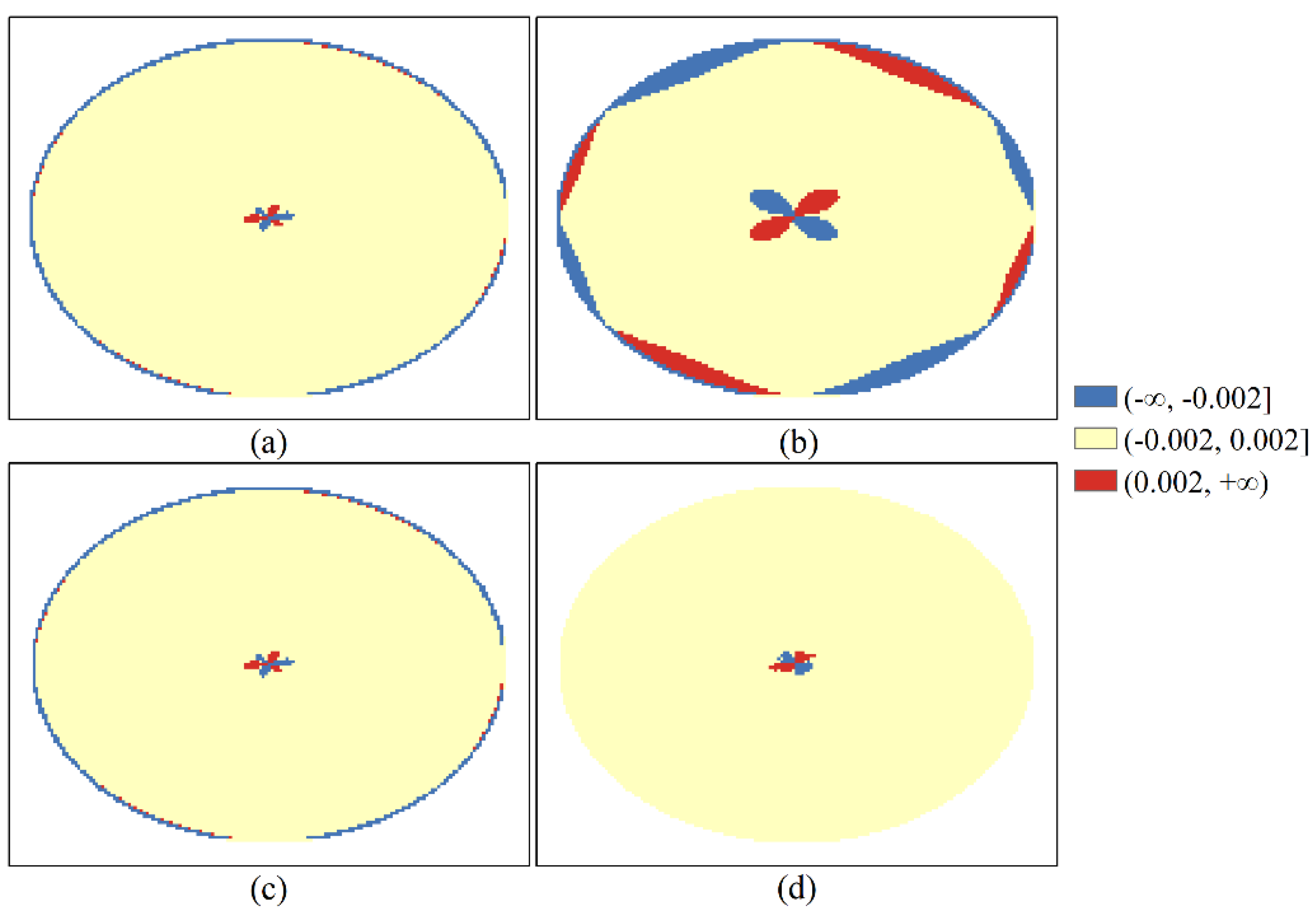
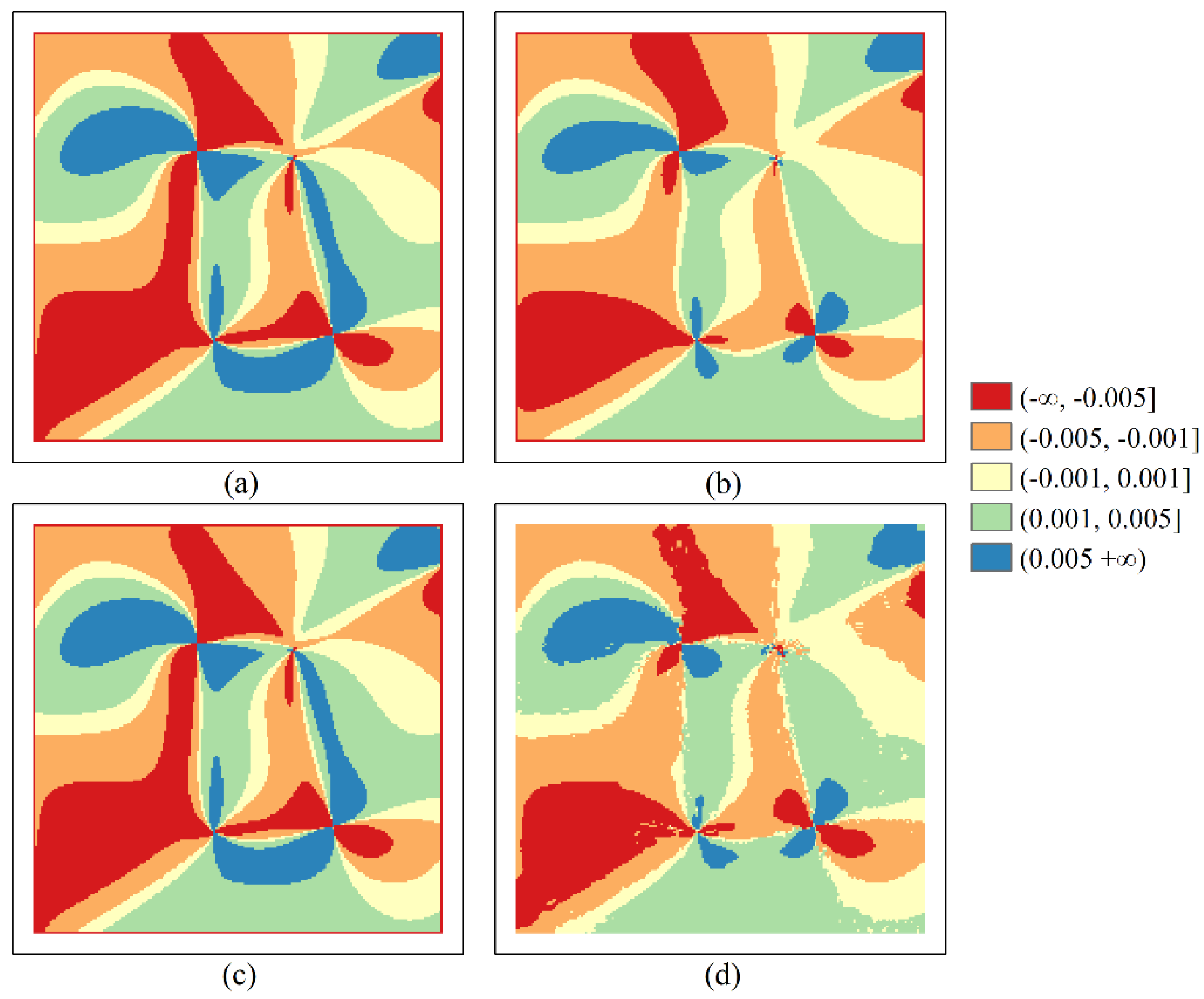
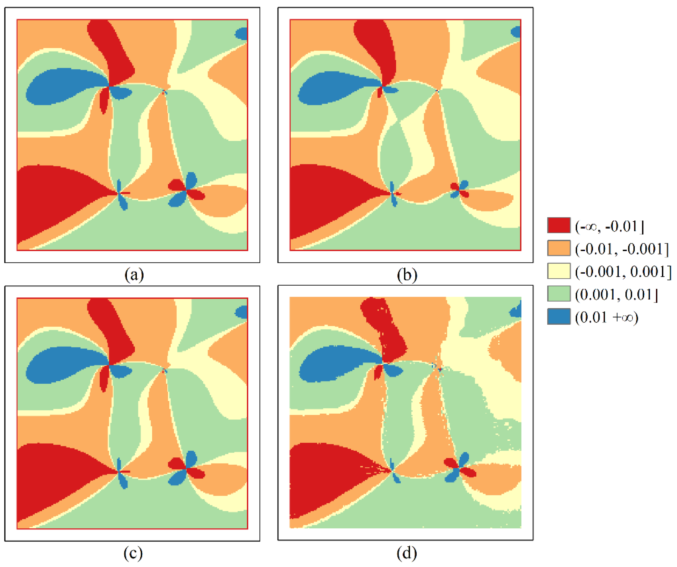
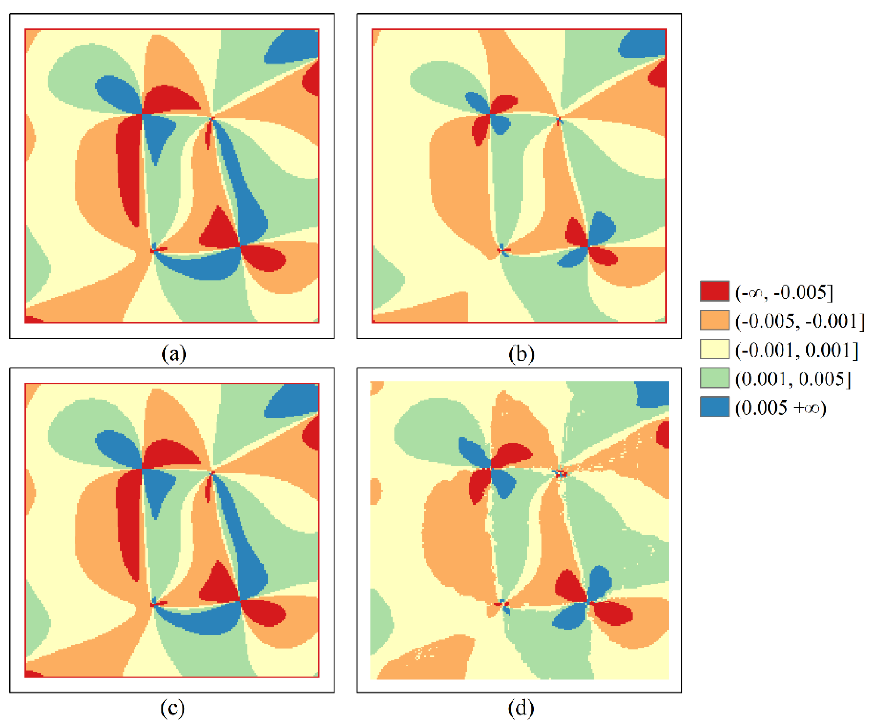
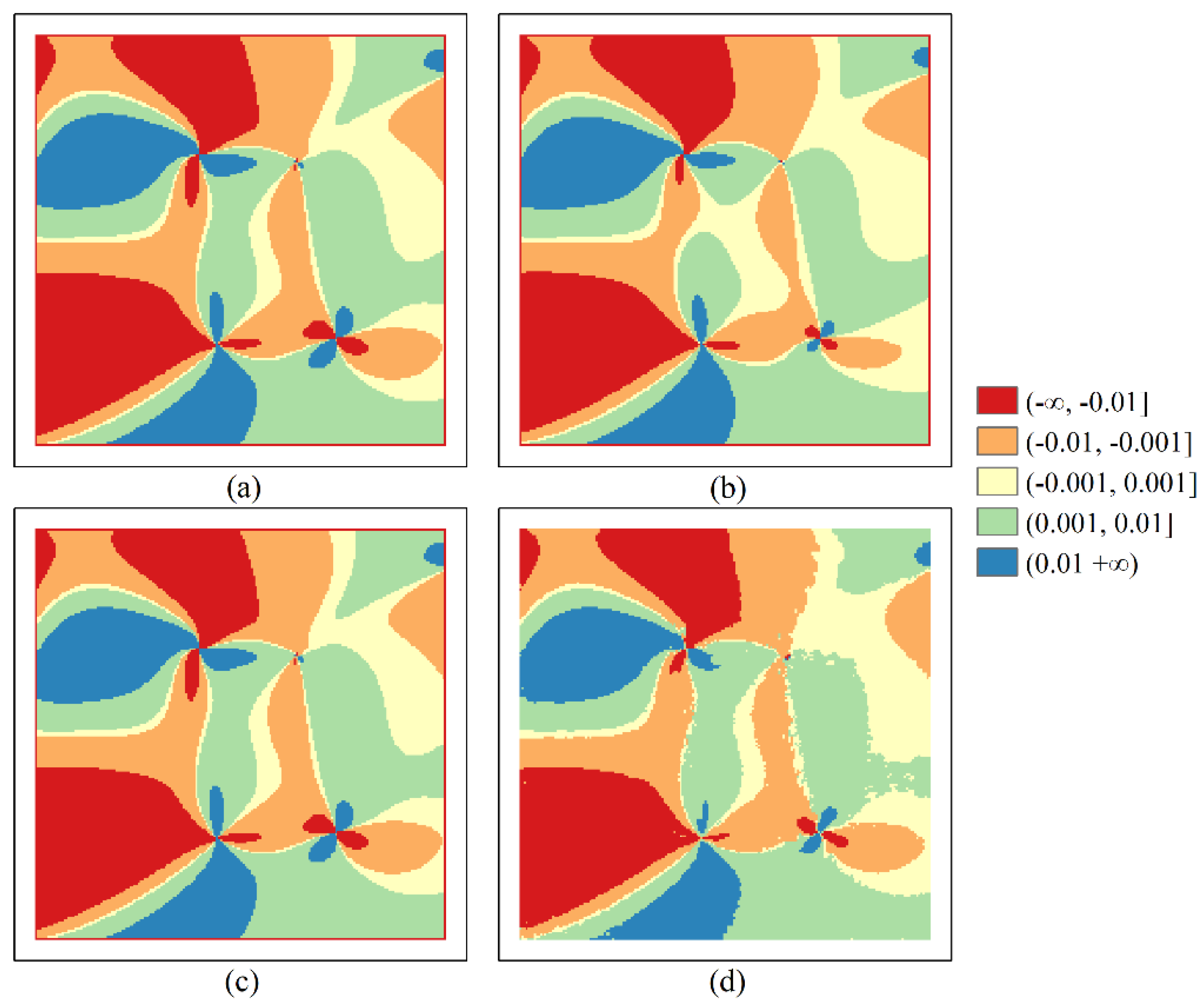
The results of the spatial distributions of the residual values on the mathematical surfaces and of the estimated C values on the real-world terrain show the expected distribution patterns, and discrete patterns and some anomalous distributions. For E1, E2, E3, and E4, the results in Table 6 show that the number of the residual values between −∞ and −0.002 and between 0.002 and +∞ for the Evans and Shary algorithms was 563 and 80, respectively. The number of the residual values between −∞ and −0.002 and 0.002 and between 0.002 and +∞ for the Zevenbergen algorithm was 1288 and 804, respectively. The number of the residual values between −∞ and −0.002 and between 0.002 and +∞ for the new algorithm was 42 and 45, respectively. For the Evans and Shary algorithms, the number of the residual value between −∞ and −0.005 and between 0.005 and +∞ on G1 was 3492 and 3384, respectively. The number of the residual value between −∞ and −0.005 and between 0.005 and +∞ on G2 was 8105 and 4710, respectively. The number of the residual value between −∞ and −0.01 and between 0.01 and +∞ on G3 was 5660 and 2112, respectively. The number of the residual value between −∞ and −0.01 and between 0.01 and +∞ on G4 was 8309 and 4892, respectively.

For the Zevenbergen algorithm, the number of the residual value between −∞ and −0.005 and between 0.005 and +∞ on G1 was 1708 and 1334, respectively. The number of the residual value between −∞ and −0.005 and between 0.005 and +∞ on G2 was 6037 and 2363, respectively. The number of the residual value between −∞ and −0.01 and between 0.01 and +∞ on G3 was 5267 and 1554, respectively. The number of the residual value between −∞ and −0.01 and between 0.01 and +∞ on G4 was 7843 and 4477, respectively. For the new algorithm, the number of the residual value between −∞ and −0.005 and between 0.005 and +∞ on G1 was 1341 and 1471, respectively. The number of the residual value between −∞ and −0.005 and between 0.005 and +∞ on G2 was 2846 and 5603, respectively. The number of the residual value between −∞ and −0.01 and between 0.01 and +∞ on G3 was 4673 and 1908, respectively. The number of the residual value between −∞ and −0.01 and between 0.01 and +∞ on G4 was 7356 and 4551, respectively. These results demonstrate that the number of large errors of the new algorithm is generally lower than that of the other comparison algorithms.

From Table 7, we can see that the proportions of the large errors obtained by the Evans, Zevenbergen, and Shary and the proposed method were 4.28%, 13.92%, 4.28%, and 0.58%, respectively. The results in Table 8 show that the proportion of large errors of the new algorithm reduced by 86.45%, 95.83%, and 86.45% of that of the Evans, Zevenbergen, and Shary algorithms, respectively. For the Evans, Zevenbergen, and Shary and the proposed methods, the proportions of large errors on G1 were 17.19%, 7.61%, 17.19%, and 7.03%, respectively. The proportions of large errors on G2 were 32.04%, 21.00%, 32.04%, and 21.12%, respectively. The proportions of large errors on G3 were 19.43%, 17.05%, 19.43%, and 16.45%, respectively. The proportions of large errors on G4 were 33.00%, 30.80%, 33.00%, and 29.77%, respectively. The results in Table 8 show that the proportion of large errors of the new approach reduced by 59.10%, 34.08%, 15.34%, and 9.79% of that of the Evans and Shary algorithms on G1, G2, G3, and G4, respectively. The proportion of large error of the new approach reduced by 7.62%, −0.57%, 3.52%, and 3.34% of that of the Zevenbergen algorithm on G1, G2, G3, and G4, respectively. These results demonstrate that the proportion of large errors of the new algorithm is generally lower than that of other comparison algorithms.

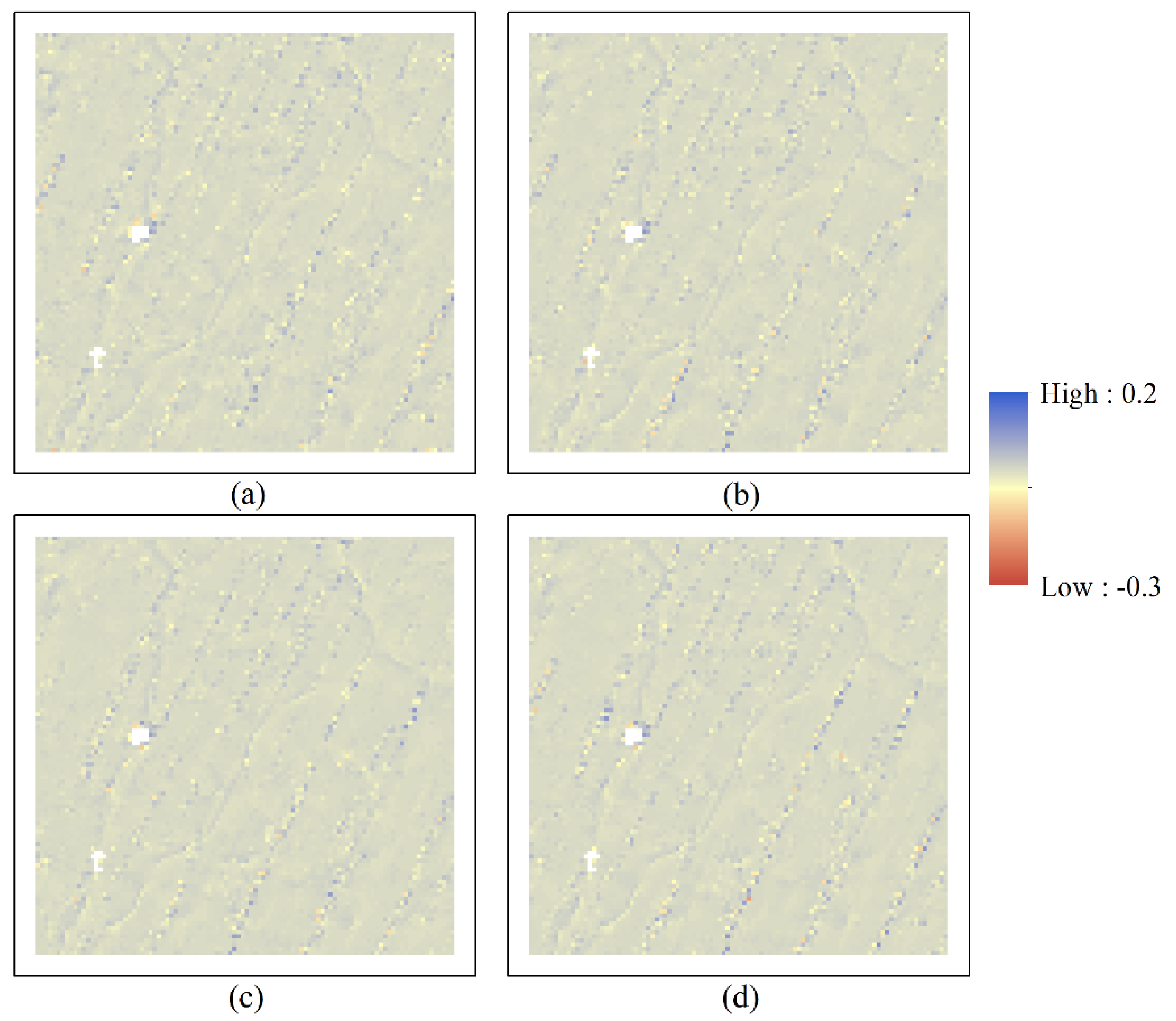
For E1, E2, E3, and E4, the proportion of residual values of the new approach between −0.002 and 0.002 increased by 3.87% compared to the Evans and Shary approaches. The proportion of residual values of the new approach between −0.002 and 0.002 increased by 15.50% compared to the Zevenbergen algorithm. Combing the results in Figure 9, we can see that the residual value of the new approach was mainly distributed between −0.002 and 0.002, and was smaller than that of the comparison algorithms on E1, E2, E3, and E4. For the abovementioned order of Gauss surfaces, the proportion of residual values of the new approach between −0.001 and 0.001 increased by 21.03%, 16.29%, 16.06%, and 21.39% compared to the Evans and Shary approaches, respectively. Compared to the Zevenbergen algorithm, the proportion of residual values of the new approach between −0.001 and 0.001 reduced by 6.60%, 6.47%, 10.47%, and 9.29%, respectively. Combing the results in Figure 10, Figure 11, Figure 12 and Figure 13, we can see that the spatial error of the proposed method was much higher than that of the Evans and Shary algorithms, and slightly lower than that of the Zevenbergen algorithm on G1, G2, G3, and G4 on the whole. Therefore, the performance of the new approach is generally better than that of the comparison algorithms on the ellipsoid and Gauss surfaces.

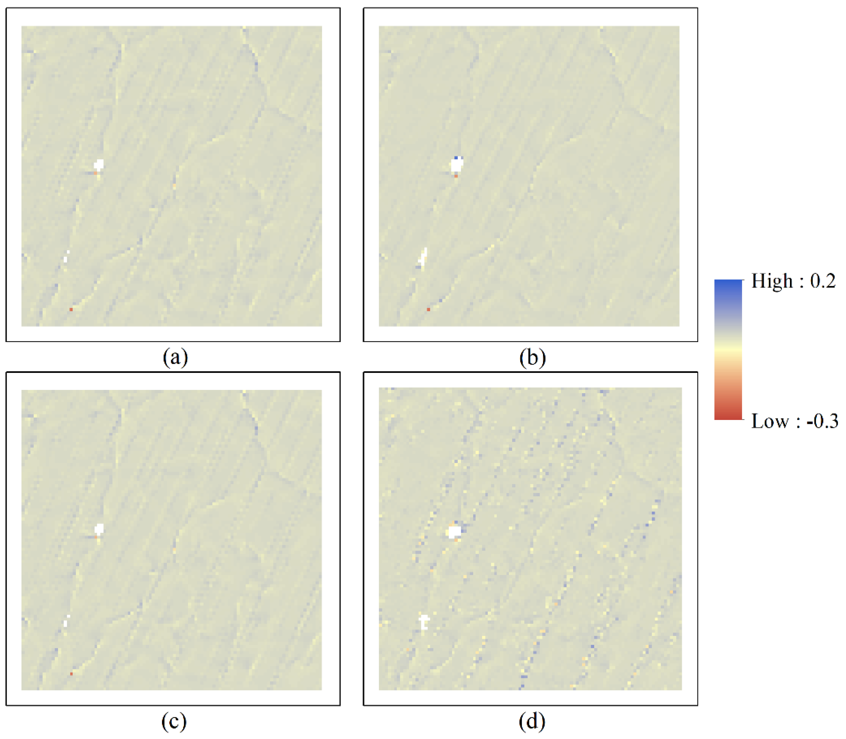
From Figure 14 and Figure 16, we can see that the C value of the proposed algorithm was slightly higher than that of the Evans, Zevenbergen, and Shary algorithms on the ridges of extremely complicated terrain surfaces, which symbolized the area with obvious topographic relief. The new algorithm has a relative advantage over the selected comparison methods in gullies. Generally speaking, the FPN-based algorithm produces plausible outcomes, which conform to the real terrain. Because of the lack of field measurements of the partial derivatives, the quantitative evaluation of the proposed algorithm could not be simulated.

5.3. Consistent Simulation Results

From Table 4, we can see how the accuracy of the new approach varied depending on the threshold value for cutting up the flow line over the FPN. For E1, the RMSE of the FPN-based algorithm was 0.0014, 0.0014, 0.0014, and 0.0015 m under the threshold values of 30, 50, 100, and 150 m, respectively. The MAE of the newly proposed algorithm was 0.0002 m under the different threshold values. For G1, the RMSE of the FPN-based algorithm was 0.0044, 0.0043, 0.0043, and 0.0043 m under the threshold values of 30, 50, 100, and 150 m, respectively. The MAE of the newly proposed algorithm was 0.0027, 0.0025, 0.0025, and 0.0025 m under different threshold values. Combined with the results shown in Figure 14, the accuracy of the new algorithm was generally invariant with the change of the cutting-up threshold for the ellipsoid, Gauss, and real-world surfaces. Therefore, the proposed algorithm achieved the consistent simulation results.

6. Conclusions

In this paper, we propose a new approach to simulating the flow path curvature (C) using a vector-based method. This approach utilizes a new FPN-C method to derive C from the flow path network (FPN). The new algorithm aims to enhance the accuracy of simulating C and avoid interpolation errors, as well as being the choice of calculation algorithm for practical applications.

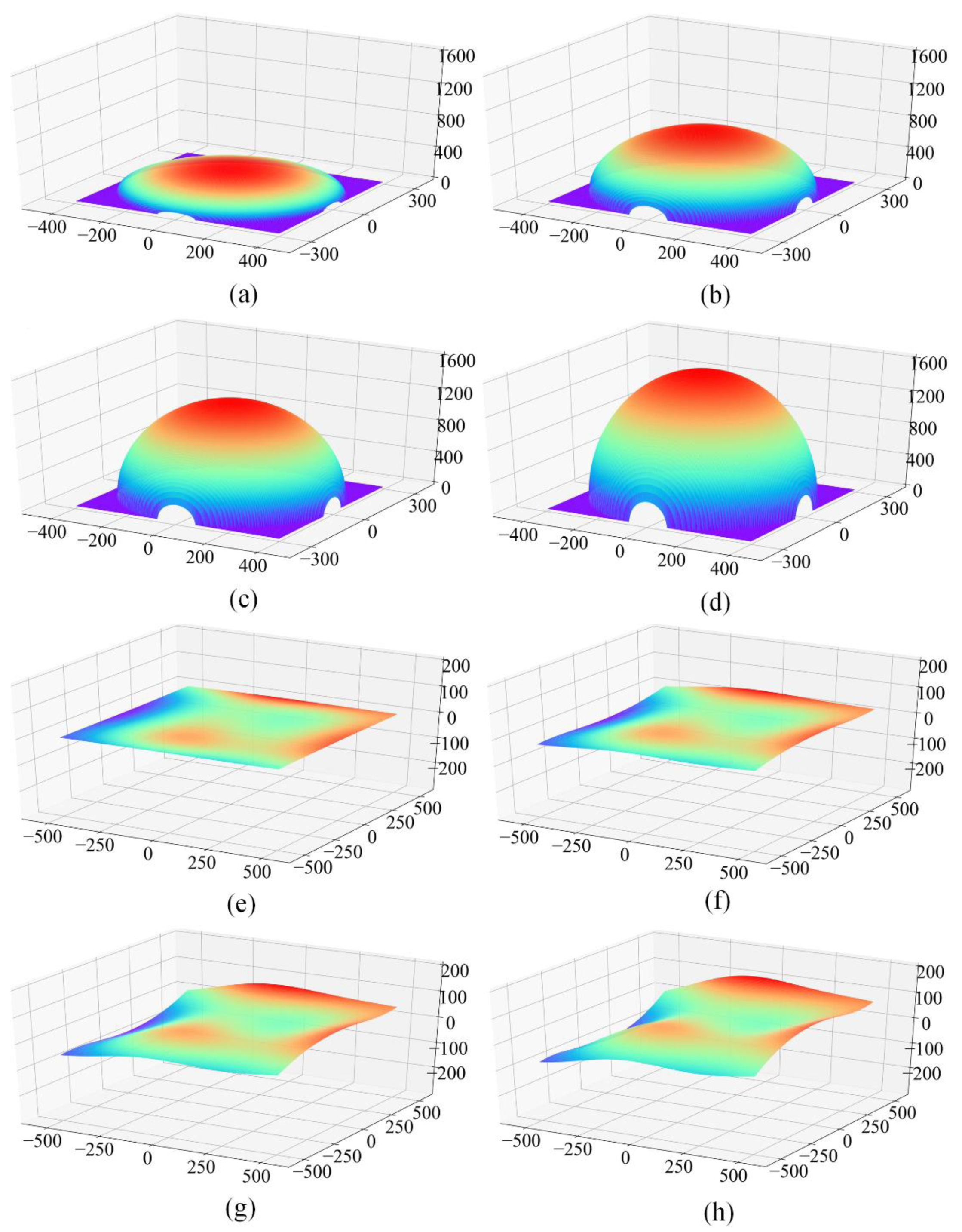
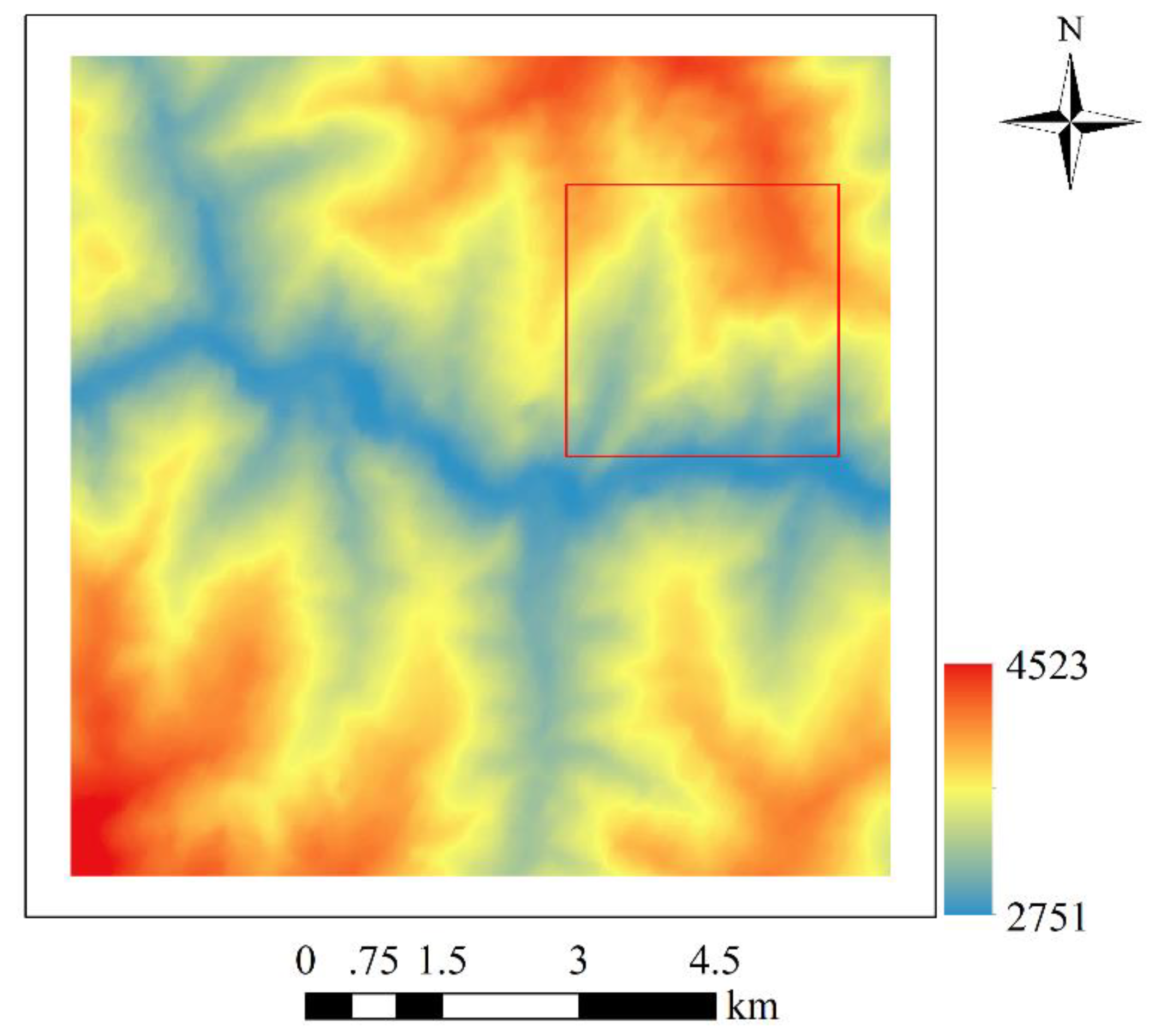
The presented method was implemented on the mathematical ellipsoid and Gauss surface models for a quantitative evaluation. Then, it was applied to a hilly plateau and mountainous region, located in the central Ganzi Tibetan Autonomous Prefecture of Sichuan Province, as a qualitative assessment. The results demonstrated that the new algorithm can obtain a relatively good result on different terrain surfaces. The new approach generally performed better than the comparison algorithms on the two above-mentioned surfaces. It was validated by both the quantitative evaluation (RMSE and MAE) and qualitative assessment (the visual comparison of the spatial distribution of the simulated C values on the mathematical and real-world surface). The RMSE and MAE of the new method were 0.0014 and 0.0002 m, reduced by up to 42% and 82% of that of the comparison algorithms on the ellipsoid surface, respectively. The RMSE and MAE of the presented method were 0.0043 and 0.0025 m at best, reduced by up to 35% and 14% of that of the comparison algorithms on the Gauss surface, respectively. For the ellipsoid surfaces, the residual value of the new approach was mainly distributed between −0.002 and 0.002 which was smaller than that of the comparison algorithms. The proportion of large errors of the new algorithm was 0.58%, reduced by up to 95.83% of that of the comparison algorithms. For the Gauss surfaces, the proportion of large errors of the new algorithm was 7.03% at best, reduced by up to 59.10% of that of the comparison algorithms. Moreover, this new approach can achieve consistent simulation results.

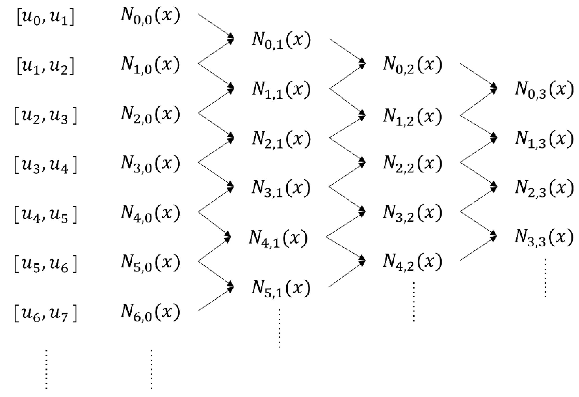
However, the vector-based flow line requires a high computing power in practical applications, especially in large DEMs. Therefore, the optimization and parallelization of this algorithm will be the focus of our future work. In addition, the B-spline interpolation method does not pass through the point used for interpolation. Thus, there may be a better algorithm to further enhance the accuracy when estimating the flow path curvature, which will be addressed in our future work as well. We will also continue to improve the calculation of the flow path curvature for the karstic or glacier type relief surfaces.

References

1. Curtis, L.; Doornkamp, J.; Gregory, K. The description of relief in field studies of soils. J. Soil Sci. 1965, 16, 16–30. [Google Scholar] [CrossRef]
2. Speight, J. Parametric description of land form. In Land Evaluation: Papers of a CSIRO Symposium; Stewart, G.A., Ed.; Macmillan: Melbourne, Australia, 1968; pp. 239–250. [Google Scholar]
3. Zhou, Q.; Liu, X. Digital Terrain Analysis; Science Press: Beijing, China, 2006. [Google Scholar]
4. Peckham, S.D. Profile, plan and streamline curvature: A simple derivation and applications. In Proceedings of the Proceedings of Geomorphometry, Redlands, CA, USA, 7–11 September 2011. [Google Scholar]
5. Minár, J.; Jenčo, M.; Evans, I.S.; Minár, J.; Kadlec, M.; Krcho, J.; Pacina, J.; Burian, L.; Benová, A. Third-order geomorphometric variables (derivatives): Definition, computation and utilization of changes of curvatures. Int. J. Geogr. Inf. Sci. 2013, 27, 1381–1402. [Google Scholar] [CrossRef]
6. Goldgof, D.; Huang, T.; Lee, H. Terrain analysis from curvature profiles. Int. J. Imaging Syst. Technol. 2005, 2, 169–182. [Google Scholar] [CrossRef]
7. Arundel, S.T.; Li, W.; Zhou, X. The effect of resolution on terrain feature extraction. Peer J. Prepr. 2018, 6, e27072v1. [Google Scholar] [CrossRef]
8. Jenny, B.; Jenny, H.; Hurni, L. Terrain generalization with multi-scale pyramids constrained by curvature. Cartogr. Geogr. Inf. Sci. 2011, 38, 110–116. [Google Scholar] [CrossRef]
9. Safanelli, J.L.; Poppiel, R.R.; Ruiz, L.F.C.; Bonfatti, B.R.; Mello, F.A.d.O.; Rizzo, R.; Demattê, J.A.M. Terrain Analysis in Google Earth Engine: A Method Adapted for High-Performance Global-Scale Analysis. ISPRS Int. J. Geo-Inf. 2020, 9, 400. [Google Scholar] [CrossRef]
10. Xia, X.; Liang, Q. A new depth-averaged model for flow-like landslides over complex terrains with curvatures and steep slopes. Eng. Geol. 2018, 234, 174–191. [Google Scholar] [CrossRef]
11. Wu, J.; Ye, L.; Wu, C.; Chang, Q.; Xin, Z.; Zhang, C.; Zhou, H. Spatial variation of channel head curvature in small mountainous watersheds. Hydrol. Res. 2019, 50, 1251–1266. [Google Scholar] [CrossRef]
12. Nagaveni, C.; Kumar, K.P.; Ravibabu, M.V. Evaluation of TanDEMx and SRTM DEM on watershed simulated runoff estimation. J. Earth Syst. Sci. 2018, 128, 2. [Google Scholar] [CrossRef] [Green Version]
13. Hooshyar, M.; Wang, D.; Kim, S.; Medeiros, S.C.; Hagen, S.C. Valley and channel networks extraction based on local topographic curvature andk-means clustering of contours. Water Resour. Res. 2016, 52, 8081–8102. [Google Scholar] [CrossRef] [Green Version]
14. Niedda, M. Upscaling hydraulic conductivity by means of entropy of terrain curvature representation. Water Resour. Res. 2004, 40, 1–16. [Google Scholar] [CrossRef] [Green Version]
15. Yu, B.; Liu, G.; Liu, Q.; Huang, C.; Li, H. Effects of topographic domain and land use on spatial variability of deep soil moisture in the semi-arid Loess Plateau of China. Hydrol. Res. 2019, 50, 1281–1292. [Google Scholar] [CrossRef] [Green Version]
16. Ngunjiri, M.W.; Libohova, Z.; Minai, J.O.; Serrem, C.; Owens, P.R.; Schulze, D.G. Predicting soil types and soil properties with limited data in the Uasin Gishu Plateau, Kenya. Geoderma Reg. 2019, 15, e00210. [Google Scholar] [CrossRef]
17. Hartsock, N.J.; Mueller, T.G.; Karathanasis, A.D.; Cornelius, P.L. Interpreting soil electrical conductivity and terrain attribute variability with soil surveys. Precis. Agric. 2005, 6, 53–72. [Google Scholar] [CrossRef]
18. Dai, Z.X.; Shi, X.C. The influence of terrain curvature on coal and gas outburst. Meitan Xuebao/J. China Coal Soc. 2012, 37, 1541–1546. [Google Scholar]
19. Fischer, J.T.; Kowalski, J.; Pudasaini, S.P. Topographic curvature effects in applied avalanche modeling. Cold Reg. Sci. Technol. 2012, 74–75, 21–30. [Google Scholar] [CrossRef]
20. Sun, X.; Chen, J.; Bao, Y.; Han, X.; Zhan, J.; Peng, W. Landslide Susceptibility Mapping Using Logistic Regression Analysis along the Jinsha River and Its Tributaries Close to Derong and Deqin County, Southwestern China. ISPRS Int. J. Geo-Inf. 2018, 7, 438. [Google Scholar] [CrossRef] [Green Version]
21. Orwat, J. Linear regression equation of mining terrain curvatures caused by hard coal excavation from a few seams and their approximated values by the use of smoothed spline. IOP Conf. Ser. Mater. Sci. Eng. 2019, 477, 012042. [Google Scholar] [CrossRef]
22. Martin, R.; Brabyn, L.; Potter, M. Sensitivity of GIS-derived terrain variables at multiple scales for modelling stoat (Mustela erminea) activity. Appl. Geogr. 2011, 31, 770–779. [Google Scholar] [CrossRef]
23. Gomes, R.; Denton, A.; Franzen, D. Quantifying Efficiency of Sliding-Window Based Aggregation Technique by Using Predictive Modeling on Landform Attributes Derived from DEM and NDVI. ISPRS Int. J. Geo-Inf. 2019, 8, 196. [Google Scholar] [CrossRef] [Green Version]
24. Schmidt, J.; Evans, I.S.; Brinkmann, J. Comparison of polynomial models for land surface curvature calculation. Int. J. Geogr. Inf. Sci. 2003, 17, 797–814. [Google Scholar] [CrossRef]
25. Evans, I. General geomorphometry. Derivatives of altitude and descriptive statistic. In Spatial Analysis Geomorphology; Chorley, R.J., Ed.; Methuen and Co.: London, UK, 1972; pp. 17–90. [Google Scholar]
26. Shary, P.A. Topographic method of second deviatives. In The Geometry of Earth Surface Structures; Stepanov, I.N., Ed.; Pushchino Research Centre Press: Pushchino, Russian, 1991; pp. 28–58. [Google Scholar]
27. Wood, J.D. The geomorphological Characterization of Digital Elevation Models. Ph.D. Thesis, University of Leicester, Leicester, UK, 1996. [Google Scholar]
28. Speight, J.G. A parametric approach to landform regions. Prog. Geomorphol. 1974, 7, 213–230. [Google Scholar]
29. Papo, H.B.; Gelbman, E. Digital terrain models for slopes and curvatures. Photogramm. Eng. Remote Sens. 1984, 50, 695–701. [Google Scholar]
30. Shary, P.A.; Sharaya, L.S.; Mitusov, A.V. Fundamental quantitative methods of land surface analysis. Geoderma 2002, 107, 1–32. [Google Scholar] [CrossRef]
31. Krebs, P.; Stocker, M.; Pezzatti, G.B.; Conedera, M. An alternative approach to transverse and profile terrain curvature. Int. J. Geogr. Inf. Sci. 2015, 29, 643–666. [Google Scholar] [CrossRef]
32. Krcho, J. Georelief as a subsystem of landscape and the influence of morphometric parameters of georelief on spatial differentiation of landscape-ecological processes. Ecology (CSFR) 1991, 10, 115–157. [Google Scholar]
33. Evans, I.S.; Cox, N.J. Relations between land surface properties: Altitude, slope and curvature. In Process Modelling and Landform Evolution. Lecture Notes in Earth Sciences; Hergarten, S., Neugebauer, H.J., Eds.; Springer: Berlin/Heidelberg, Germany, 1999; Volume 78. [Google Scholar]
34. Evans, I.S. Land surface derivatives: History, calculation and further development. In Proceedings of the Geomorphometry, Nanjing, China, 16–20 October 2013. [Google Scholar]
35. Shary, P.A. Land surface in gravity points classification by a complete system of curvatures. Math. Geol. 1995, 27, 373–390. [Google Scholar] [CrossRef]
36. Marián Jenčo, J.P.; Shary, P. Terrain skeleton and local morphometric variables: Geosciences and computer vision technique. In Advances in Geoinformation Technologies; Horák, J., Ed.; Ostrava VŠB-Technical University of Ostrava: Ostrava, Czech Republic, 2009. [Google Scholar]
37. Pradhan, K.; Guha, A. Fluid dynamics of a bifurcation. Int. J. Heat Fluid Flow 2019, 80, 108483. [Google Scholar] [CrossRef]
38. Pathak, M.; Dewan, A.; Dass, A.K. Effect of streamline curvature on flow field of a turbulent plane jet in cross-flow. Mech. Res. Commun. 2007, 34, 241–248. [Google Scholar] [CrossRef]
39. Yang, X.; Tucker, P.G. Assessment of turbulence model performance: Large streamline curvature and integral length scales. Comput. Fluids 2016, 126, 91–101. [Google Scholar] [CrossRef] [Green Version]
40. Tjerry, S.; Fredsøe, J. Calculation of dune morphology. J. Geophys. Res. Earth Surf. 2005, 110, F04013. [Google Scholar] [CrossRef]
41. Bagheri, S.; Kabiri-Samani, A. Simulation of free surface flow over the streamlined weirs. Flow Meas. Instrum. 2020, 71, 101680. [Google Scholar] [CrossRef]
42. Foroutan, M.; Kompanizare, M.; Ehsani, A.H. Semiautomatic morphometric land surface segmentation of an arid mountainous area using DEM and self-organizing maps. Arab. J. Geosci. 2013, 6, 4795–4810. [Google Scholar] [CrossRef]
43. Florinsky, I.V. Accuracy of local topographic variables derived from digital elevation models. Int. J. Geogr. Inf. Sci. 1998, 12, 47–62. [Google Scholar] [CrossRef]
44. Evans, I.S. An integrated system of terrain analysis and slope mapping. Z. Geomorphol. (Suppl. Band) 1980, 36, 274–295. [Google Scholar]
45. Florinsky, I.V. Computation of the third-order partial derivatives from a digital elevation model. Int. J. Geogr. Inf. Sci. 2009, 23, 213–231. [Google Scholar] [CrossRef]
46. Zevenbergen, L.W.; Thorne, C.R. Quantitative analysis of land surface topography. Earth Surf. Process. Landf. 1987, 12, 47–56. [Google Scholar] [CrossRef]
47. Moore, I.D.; Gessler, P.E.; Nielsen, G.A.; Peterson, G.A. Soil Attribute Prediction Using Terrain Analysis. Soil Sci. Soc. Am. J. 1993, 57, NP. [Google Scholar] [CrossRef]
48. Schmidt, J.; Dikau, R. Extracting geomorphometric attributes and objects from digital elevation models-Semantics, methods, future needs. In GIS for Earth Surface Systems: Analysis and Modeling of the Natural Environment; Dikau, R., Saurer, H., Eds.; Gebrüder Borntraeger Verlag: Berlin, Germany, 1999; pp. 153–173. [Google Scholar]
49. Chen, Y.; Zhou, Q.; Li, S.; Meng, F.; Bi, X.; Wilson, J.P.; Xing, Z.; Qi, J.; Li, Q.; Zhang, C. The simulation of surface flow dynamics using a flow-path network model. Int. J. Geogr. Inf. Sci. 2014, 28, 2242–2260. [Google Scholar] [CrossRef]
50. Zhou, Q.; Pilesjö, P.; Chen, Y. Estimating surface flow paths on a digital elevation model using a triangular facet network. Water Resour. Res. 2011, 47, W07522. [Google Scholar] [CrossRef]
51. Tarboton, D. Terrain Analysis Using Digital Elevation Models in Hydrology. In Proceedings of the 23rd ESRI International Users Conference, San Diego, CA, USA, 7–11 July 2003. [Google Scholar]
52. Tarboton, D.G. A new method for the determination of flow directions and upslope areas in grid digital elevation models. Water Resour. Res. 1997, 33, 662–670. [Google Scholar] [CrossRef] [Green Version]
53. Kienzle, S. The Effect of DEM Raster Resolution on First Order, Second Order and Compound Terrain Derivatives. Trans. GIS 2004, 8, 83–111. [Google Scholar] [CrossRef]
54. Segeth, K. Polyharmonic splines generated by multivariate smooth interpolation. Comput. Math. Appl. 2019, 78, 3067–3076. [Google Scholar] [CrossRef]
55. Bauer, F.; Grüne, L.; Semmler, W. Adaptive spline interpolation for Hamilton–Jacobi–Bellman equations. Appl. Numer. Math. 2006, 56, 1196–1210. [Google Scholar] [CrossRef]
56. Li, H.; Qin, X.; Zhao, D.; Chen, J.; Wang, P. An improved empirical mode decomposition method based on the cubic trigonometric B-spline interpolation algorithm. Appl. Math. Comput. 2018, 332, 406–419. [Google Scholar] [CrossRef]
57. Rao, K.D.; Ghosh, S.; Das, S.; Kumar, M.R. A fractional calculus based generalized design scheme for very low-frequency oscillator using spline interpolation with sensitivity analysis. Commun. Nonlinear Sci. Numer. Simul. 2019, 79, 104917. [Google Scholar] [CrossRef]
58. Zhao, D.; Huang, Z.; Li, H.; Chen, J.; Wang, P. An improved EEMD method based on the adjustable cubic trigonometric cardinal spline interpolation. Digit. Signal Process. 2017, 64, 41–48. [Google Scholar] [CrossRef]
59. Tan, B.; Huang, M.; Zhu, Q.; Guo, Y.; Qin, J. Detection and correction of laser induced breakdown spectroscopy spectral background based on spline interpolation method. Spectrochim. Acta Part B At. Spectrosc. 2017, 138, 64–71. [Google Scholar] [CrossRef]
60. Othman, M.M.; Mohamed, A.; Hussain, A. Fast evaluation of available transfer capability using cubic-spline interpolation technique. Electr. Power Syst. Res. 2005, 73, 335–342. [Google Scholar] [CrossRef]
61. Sandwell, D.T. Biharmonic spline interpolation of GEOS-3 and SEASAT altimeter data. Geophys. Res. Lett. 1987, 14, 139–142. [Google Scholar] [CrossRef] [Green Version]
62. Toraichi, K.; Mori, R.; Kamada, M.; Ishiuchi, S.; Yang, S. Improvement of Video Hardcopy Image Quality by Using Spline Interpolation. Syst. Comput. Jpn. 1989, 20, 13–24. [Google Scholar] [CrossRef]
63. Liu, Z.W.; Chen, R.S.; Chen, J.Q. Adaptive sampling cubic-spline interpolation method for efficient calculation of monostatic RCS. Microw. Opt. Technol. Lett. 2008, 50, 751–755. [Google Scholar] [CrossRef]
64. Busan, S.; Othman, M.M.; Musirin, I.; Mohamed, A.; Hussain, A. Determination of available transfer capability by means of Ralston’s method incorporating cubic-spline interpolation technique. Eur. Trans. Electr. Power 2011, 21, 439–464. [Google Scholar] [CrossRef]
65. Zhou, Q.; Liu, X.; Sun, Y. Terrain complexity and uncertainties in grid-based digital terrain analysis. Int. J. Geogr. Inf. Sci. 2006, 20, 1137–1147. [Google Scholar] [CrossRef]
66. Zhou, Q.; Liu, X. Error analysis on grid-based slope and aspect algorithms. Photogramm. Eng. Remote Sens. 2004, 70, 957–962. [Google Scholar] [CrossRef]
Figure 1. Flow chart of the flow path network (FPN)-based algorithm for computing C.
Ijgi 09 00510 g001
Figure 2. Flow direction over the triangular facet drawn from a random point.
Ijgi 09 00510 g002
Figure 3. Operational relationship between the basic functions.
Ijgi 09 00510 g003
Figure 4. Smoothing the flow line by the cubic B-spline interpolation method.
Ijgi 09 00510 g004
Figure 5. Fitting the circle of the grid cell by the least square algorithm.
Ijgi 09 00510 g005
Figure 6. Distribution and numbering of the 3 × 3 window (g is the resolution).
Ijgi 09 00510 g006
Figure 7. Test digital elevation model (DEM) used in this study. The red box delineates a subregion (number of the grid cells of 100 × 100) to support a visual comparison.
Ijgi 09 00510 g007
Figure 8. DEMs generated from four ellipsoid and four Gauss surfaces with various parameters: (a) E1, (b) E2, (c) E3, (d) E4, (e) G1, (f) G2, (g) G3, and (h) G4. The color indicates the change in elevation over the DEM.
Ijgi 09 00510 g008
Figure 9. Spatial distribution of the residuals of the simulated C values relative to the theoretical C values on E1, E2, E3, and E4 for the: (a) Evans, (b) Zevenbergen, (c) Shary, and (d) FPN-based methods.
Ijgi 09 00510 g009
Figure 10. Spatial distribution of the residuals of the simulated C values relative to the theoretical C values on G1 for the: (a) Evans, (b) Zevenbergen, (c) Shary, and (d) FPN-based methods.
Ijgi 09 00510 g010
Figure 11. Spatial distribution of the residuals of the simulated C values relative to the theoretical C values on G2 for the: (a) Evans, (b) Zevenbergen, (c) Shary, and (d) FPN-based methods.
Ijgi 09 00510 g011
Figure 12. Spatial distribution of the residuals of the simulated C values relative to the theoretical C values on G3 for the: (a) Evans, (b) Zevenbergen, (c) Shary, and (d) FPN-based methods.
Ijgi 09 00510 g012
Figure 13. Spatial distribution of the residuals of the simulated C values relative to the theoretical C values on G4 for the: (a) Evans, (b) Zevenbergen, (c) Shary, and (d) FPN-based methods.
Ijgi 09 00510 g013
Figure 14. The triangular facet network (TFN) and FPN of the subregion: (a) TFN and (b) FPN.
Ijgi 09 00510 g014
Figure 15. Spatial distribution of the simulated C values of the subregion for the threshold value of: (a) 100 m, (b) 150 m, (c) 200 m, and (d) 250 m.
Ijgi 09 00510 g015
Figure 16. Spatial distribution of the simulated C values of the subregion for the: (a) Evans, (b) Zevenbergen, (c) Shary, and (d) FPN-based methods.
Ijgi 09 00510 g016