Spatial Distribution of the Mexican Daisy, Erigeron karvinskianus, in New Zealand under Climate Change


Environmental and Animal Sciences Practice Pathway, Unitec Institute of Technology, Private Bag 92025, Victoria Street West, Auckland 1142, New Zealand
*
Author to whom correspondence should be addressed.
Climate 2019, 7(2), 24; https://0-doi-org.brum.beds.ac.uk/10.3390/cli7020024
Submission received: 29 November 2018
/
Revised: 27 January 2019
/
Accepted: 28 January 2019
/
Published: 30 January 2019
Abstract
:The invasive species Erigeron karvinskianus or Mexican daisy is considered a significant weed that impacts native forest restoration efforts in New Zealand. Mapping the potential distribution of this species under current and future predicted climatic conditions provides managers with relevant information for developing appropriate management strategies. Using occurrences available from global and local databases, spatial distribution characteristics were analyzed using geostatistical tools in ArcMap to characterize current distribution. Species distribution modeling (SDM) using Maxent was conducted to determine the potential spatial distribution of E. karvinskianus worldwide and in New Zealand with projections into future climate conditions. Potential habitat suitability under future climatic conditions were simulated using greenhouse gas emission trajectories under the Representative Concentration Pathway (RCP) models RCP2.6, RCP4.5, RCP6.0 and RCP8.5 for years 2050 and 2070. Occurrence data were processed to minimize redundancy and spatial autocorrelation; non-correlated environmental variables were determined to minimize bias and ensure robust models. Kernel density, hotspot and cluster analysis of outliers show that populated areas of Auckland, Wellington and Christchurch have significantly greater concentrations of E. karvinskianus. Species distribution modeling results find an increase in the expansion of range with higher RCP values, and plots of centroids show a southward movement of predicted range for the species.
1. Introduction
Mexican Daisy (Erigeron karvinskianus DC.) is reported as an invasive plant species throughout warm-temperate, subtropical and tropical parts of the world [1], including India [2], Africa [3], Australia [4], Japan [5], northwest Himalayas [6] and Europe [7,8]. Classified as an invasive weed, it is an identified problem in Hawaii [9,10], La Réunion [11] and New Zealand [12,13]. The species was first recorded in New Zealand in 1940 [12,13] and is now found to be established and thriving in North Island, South Island and Stewart Island [13,14], with numerous patches found in the relatively populated Auckland Region [12,15].
The species is known to be associated with anthropogenic disturbance, particularly in habitats such as rock walls, archaeological sites, roadside banks, and wasteland [1,4,8,13,16,17,18] but is also increasingly invading native ecosystems including native and replanted forests, wetlands and riparian zones [11,16,19]. It can form dense mats that can rapidly stifle young plants [1,9], with serious impacts on projects involving revegetation or replanting of areas. This in turn may require significant resources for clearing, preparation and maintenance to ensure the growth and survival of replanted species. The plant’s ability to spread at a rapid rate when introduced further increases its importance in ecological restoration efforts [13]. Characteristics of the Mexican daisy that enhance the risk of invasion, establishment and spread into unoccupied areas include wide climatic tolerance [1,2], abundant seeds highly suitable for wind dispersion or other transport vectors [1] and potential reproduction via adventitious rooting of stem fragments [1]. These factors improve its ability to adversely affect regenerating forests [19], which is a major concern in New Zealand.
New Zealand is an isolated archipelago with unique endemic flora and fauna threatened by the establishment and spread of highly invasive species [20]. The great value the country exerts in protecting its remaining biodiversity resulted in efforts to address the presence of weeds and the prevention of their establishment and diffusion. At the national level, the Department of Conservation lists the Mexican daisy as an unwanted organism, belonging to Category C of weeds characterized as “potentially troublesome that should not be spread” with “small infestations requiring removal” and is listed on the National Pest Plant Accord (NPPA) as an Unwanted Organism [21]. This classification formally describes the Mexican daisy as a threat to grassland, riverbank and cliff ecosystems [22]. At local or regional levels, policy instruments such as the Regional Pest Management Strategies were developed and enacted by Regional Councils to deal with biosecurity issues including weeds [23]. In the Auckland Region, the Mexican daisy is listed as a Surveillance species, a classification identifying the plant as a potential threat to the biodiversity of the area, with prohibitions on its distribution, sale and propagation to prevent establishment and diffusion [24]. Action recommended for initial patches is immediate removal or eradication [25].
It is recognized that weeds such as the Mexican daisy are capable of rapid shift ranges, adaptability and easy establishment [26]. To describe the current range of the plant, spatial distribution characteristics of the Mexican daisy at global, country and local area extents were mapped using ArcMap v10.5.2 and geostatistical tools used for analysis of occurrence data. The global map of current distribution and results of spatial analysis provide an overview of its native and invaded range as well as spatial information comparing distribution between different countries and regional areas of concern. Worldwide patterns of distribution, when presented as hotspots or clustering, provide countries, regions or organizations with initial risk assessments associated with invasive species and may also identify invasive pathways [27]. The plant’s highly invasive characteristics are worsened by the availability of propagules throughout most of New Zealand as well as constant disturbances such as anthropogenic, soil and vegetation cover changes that facilitate establishment [27]. Predicting and mapping the potential distribution of such an invasive species under current and future predicted climatic conditions will provide the country’s national and local managers with relevant information and knowledge for project planning, development of relevant strategies and management protocols [28,29,30].
Species distribution modeling (SDM) was used to determine the future habitat suitability distribution of important invasive species from a worldwide distribution to a smaller country or region [31,32,33]. Relevant SDM of invasive plants includes work done in the Himalayas [34], Czech Republic [35], United States [36], Canada [37] Australia [38] and New Zealand [39], among others. The resulting models and maps of predicted suitability provide valuable information that allows for the focus of attention on identified geographical areas and determines effects of relevant environmental variables. Such modeling provides knowledge for subsequent efforts in mitigating impacts brought about by the invasive species, particularly changes in range, movement into novel territories with implications on native species, habitats and resources required for addressing the impacts of the weed. This project was aimed at determining the spatial characteristics of the Mexican daisy, using global and local distribution data as well as relevant environmental data as input to several spatial modeling tools to describe current distribution and assess future potential range in New Zealand.
2. Materials and Methods
Occurrence data were sourced from the Global Biodiversity Information Facility (GBIF; http://data.gbif.org). As a database with data sourced from a wide variety of museums, projects, networks and herbaria worldwide with varying collection quality, there are recognized challenges in its use for SDM [40]. However, the ability to access and download a set of global georeferenced species occurrences makes it a valuable resource, particularly for species with no other alternative source of information. The downloaded distribution data were checked for consistency, and redundant, unnecessary and non-georeferenced data were removed. The processed Microsoft Excel data were imported into ArcMap, and the resulting distribution map was used for checking obvious errors such as redundancies and data at improbable locations, such as bodies of water or extreme latitudes.
Using the Kernel Density tool of ArcMap, a density map was created to show areas where there are greater concentrations of reported occurrences. This tool calculates magnitude of occurrences per unit area and fits a suitably smooth surface over the extent of input data points using the distances between each location. The raster output surface aids the visualization of the distribution by highlighting areas that have much greater or much lower concentration of occurrences. A planar method for generating the surface was the option used in the calculations [41,42].
The Getis-Ord Gi* [43,44] statistic implemented in the Optimized Hotspot tool of ArcMap determined characteristics of occurrences in terms of statistically significant intensities of occurrence points. The Hotspot tool aggregates occurrences into uniformly-sized cells and calculates the z-statistic with an accompanying p-value that indicates whether the cells are hotspots, coldspots or have no significance. Positive z-statistics identify cells that have high numbers of occurrences, and designates them as hot spots when the p-value is significant [45]. At the opposite scale, cells with negative z-statistics represent low numbers of occurrences and are designated as cold spots if the calculated p-value is significant [45]. To characterize the neighborhood and identify areas with characteristics of statistically significant outliers in the occurrence cells, the Optimized Cluster and Outlier tool of ArcMap that implements Anselin’s Local Moran’s I [46] was used. This tool produces cells that aggregate occurrences and use counts per cell as the variable to determine a z-score to depict outlier significance. High or low values of z-scores result in cells depicted as High-High or Low-Low cells in the map. Other results include the Low-High and High-Low cells showing the nature of the surrounding cells in relation to each other. Cells not determined by the tool to have statistically significant outliers are characterized as not significant [47].
Species distribution modeling requires a set of occurrence data and environmental variables as input. The tool Maxent (v3.4.1), implementing the maximum entropy machine learning approach, was used. Maxent is a popular tool finding widespread usage because of its performance compared to other approaches [48,49]. Maxent is based on maximum entropy that calculates inferences or predictions even under conditions where the information is not complete [50,51,52]. In SDM applications, the maximum entropy approach estimates a target distribution by calculating the probability distribution that is nearest to a uniform one under constraints determined from available data [50]. Significant applications of Maxent for modeling plant invasive species include modeling of invasive trees worldwide [53], invasive weeds in Australia [30], the Chinese fan palm [39], and the tallow tree in the Himalayas [54].
Environmental data consisted of rasters available from the WorldClim (v1.4) database that consist of 19 Bioclim environmental variables (http://worldclim.org) [55] commonly used for SDM in a wide variety of applications [56,57,58]. Current Bioclim rasters (averaged between 1960 and 1990) and available future climatic data were downloaded for 2050 and 2070 at 30-second resolution (http://www.worldclim.org/CMIP5v1). These future climatic data describe different levels of greenhouse gas trajectories as defined in the 5th IPCC report. The downloaded raster files represent Representative Concentration Pathways (RCP) with values of 2.6, 4.5, 6.0, and 8.5 (higher numbers represent greater greenhouse gas emissions, with RCP2.6 resulting in global warming by less than 2 degrees and RCP8.5 likely to lead to 4 degrees warming by 2100) for the years 2050 and 2070 [59].
The downloaded occurrence data were rarefied using the SDMToolbox v2.2 [60] in ArcMap with multiple presence points within specified range distances reduced to a single representative occurrence in order to minimize spatial autocorrelation which can affect model robustness [44,61,62]. Five sets of occurrence data were generated consisting of rarefied sets at distances of 1, 5, 10, 20, 50, and 100 km between samples. Each rarefied set was modelled in preliminary Maxent runs to determine which data set to use based on its AUC [63] performance for both worldwide and New Zealand occurrence data sets. The higher AUC score was used to select the rarefied data set for the global model, whereas for the New Zealand model, the minimal difference in AUC between the 1 km and 5 km resolutions resulted in the decision to use the 5 km data with a smaller number of samples to further minimize spatial autocorrelation [39]. The sample sizes for both models are also well above the minimum of 30 (Table 1) recommended for a range of SDM algorithms [64]. Maxent outputs a suitability map by modeling the distribution of a specific species with a selected number of environmental variables. The worldwide model was used to determine the non-correlated variables to be used for the New Zealand model. The New Zealand current model in turn was projected into future environmental conditions using RCP bioclimatic rasters. The Minimum Training Presence (MTP) threshold rule was applied in order to produce a binary raster representing the presence/absence or range of a species [65]. The MTP as a threshold in Maxent was used [66,67,68,69] primarily because of its representation of the simple interpretation of an ecological relationship between areas that are at least suitable to locations where presence is recorded. Results of the preliminary Maxent run identified the 100 k data set as most suitable for the global model and the 5 k data set for the New Zealand model (Table 1).
Bioclim rasters were further processed as it was expected that many of the climatic variables were highly correlated [60], making it difficult to determine the effects of individual variables on the Maxent model. These consisted of 19 parameters in Bioclim clipped to the New Zealand area and rasters representing elevation (https://data.linz.govt.nz/layer/51768-nz-8m-digital-elevation-model-2012/) and land cover (https://earthexplorer.usgs.gov/) [70,71], using the Biosphere 2 classification of 11 landcover types (1 Broadleaf Evergreen Trees; 2 Broadleaf Deciduous Trees; 3 Broadleaf and Needleleaf Trees; 4 Needleleaf Evergreen Trees; 5 Needleleaf Deciduous Trees; 6 Short Vegetation/Grassland; 7 Shrubs with Bare Soil; 8 Dwarf Trees and Shrubs; 9 Agriculture/Grassland; 10 Water, Wetlands; 11 Ice/Snow) and human population (https://koordinates.com/from/datafinder.stats.govt.nz/layer/8437/). Landcover, elevation and human population variables were included in the model together with bioclimatic factors to determine their effects on the Maxent jackknife outputs. Elevation was selected primarily because of observed range shifts towards higher elevation in climate changes studies [72] and to show results of variable effects on the models in the jackknife of the Maxent model while considering that New Zealand’s mountain areas contain significant habitats that may be impacted. The values of the environmental variables at each occurrence point of the selected rarefied data set were determined using the ArcMap tool Extract Multi-values from rasters (Table 2). We used SDMtoolboxv2.2 in ArcMap to check for cross-correlation of all the environmental variables at all occurrence points and determine which environmental variables to use based on the correlation coefficient [60]. Variables not correlated at coefficient less than or equal to 0.7 were included and further checked to include only those with a variance inflation factor (VIF) of less than 10 [73]. This is consistent with results that show that using simpler models with a small number of variables improves the results of projecting species distribution models [58,74,75,76]. Cross correlation of the Bioclim data resulted in the 4 layers plus landcover, population and elevation selected for use in both the global and New Zealand models (Table 2).
The global and New Zealand species distribution models were run with the 100 k and 5 k rarefied data sets, respectively. Environmental variables consisted of non-correlated current Bioclim environmental layers BIO1 (Annual Mean Temperature), BIO2 Mean Diurnal Range (Mean of monthly (max temperature–min temp)), BIO12 (Annual Precipitation), and BIO15 (Precipitation Seasonality (Coefficient of Variation), elevation, land cover and human population. The New Zealand model was projected into future climatic conditions using the downloaded RCP trajectories for the years 2050 and 2070.
Using raster calculations, subtracting the binary thresholded future rasters from current rasters resulted in four categories: Expansion in range (absence in current, presence in future), no occupancy or (absence in both current and future), occupancy or continuing (presence in current and future) and contraction in range (presence in current, absence in future). These resulting range maps provide valuable insight into areas of the country where change in range occurs. The maps also show effects of different RCP values on the range expansion or contraction of the species. The direction of presence area centroid movement was determined in ArcMap, again using the tool Distribution Changes Between Binary SDMs in the SDM toolbox. Centroid movements are plotted as vectors and represent the magnitude and direction of the movement of predicted distribution ranges. Each centroid shift vector was produced by pairwise subtraction between binary current and future rasters and also between the 2050 and 2070 binary rasters. The speed of the movement of the centroid is then calculated from the length of the centroid shift and the time difference between each pair of presence/absence rasters.
3. Results
Global spatial distribution characterization showed most of the occurrences were found in the southern region of Mexico, a large area of Europe, and the east coasts of Australia and New Zealand (Figure 1). The Optimized Hotspot Tool in ArcMap depicted the native range of the plant in Mexico and New Zealand as significant global hotspots. The rest of the world did not exhibit any significant hotspots in the generated cells analyzed. In terms of the cluster and outlier characteristics of the global distribution, the native range of the plant in Mexico showed several significant High-High cluster cells as well as Low-High outlier characterized cells. New Zealand shows several Low-High outlier cells, whereas a few High-Low outlier cells are found scattered over the world (Figure 2).
For the New Zealand distribution, the downloaded occurrence data plus the survey in the Auckland Region show that the Mexican daisy is currently prevalent in regions surrounding Auckland, Wellington and Christchurch and scattered throughout the length of North Island, and South Island, particularly at the northern end and in the Christchurch region (Figure 2). This is confirmed by kernel density modeling that shows Auckland, Wellington, the top of South Island and Christchurch to have higher densities. Areas at the eastern tip of North Island and the southwestern area of South Island do not have reported occurrences and are excluded in the resulting kernel density raster (Figure 3). Hotspot analysis using the Getis-Ord Gi* statistic show that the center of Auckland has statistically significant hotspots. Cluster and outlier analysis find Auckland with several significant Low-High outliers. Several spots of High-Low outliers are found throughout North Island and only one High-Low outlier cell in South Island was found (Figure 3).
Limiting the occurrence data set to the Auckland Region alone, there is a high density of occurrences seen particularly around the western and coastal areas. When the Optimized Hotspot tool was run, no significant hotspots were found in the distribution. Cluster and Outlier analysis, however, finds High-Low clusters in the northern and western areas of the city (Figure 3).
Species distribution modeling results from global Maxent modeling with the selected data set show the native range in Mexico and most reported invasive range of the species to be the most suitable under current conditions. Further, a significant area of New Zealand was found to be highly suitable. Coastal areas of Europe, the southern coast of Australia, the Japanese archipelago, central China, the eastern United States and southeastern Central America are also highly suitable. The presence/absence map that resulted with a threshold set at MTP level shows that a significant area of the world is predicted to be favorable for its presence or can be considered as the range of the species under current environmental conditions (Figure 4).
For the New Zealand Maxent model, jackknife analysis of variable contributions shows that human population has the greatest percentage contribution followed by land cover and BIO1 (average annual temperature). However, when permutation importance is considered, BIO1 is more important, followed by land cover and elevation. Response curves provide an idea of the variable value range or category that results in the greatest model response. The response curve for BIO1 (annual average temperature range) shows that the model has a higher response at the higher values of annual average temperature. Middle values of BIO15 (Precipitation seasonality) and lower values of BIO2 (Mean diurnal temperature range) also have more influence in the model. Lower elevations have greater effect compared to higher elevations, whereas BIO12 (average annual rainfall) has the greatest effect at lower averages, particularly when it is the only corresponding variable. For land cover, categories 1 (broadleaf evergreen forest) and 7 (shrubs with bare soil) consistently show greater effect in both response graph types (Table 3).
Using the 5 km rarefied data for New Zealand species distribution modeling reflects the distribution pattern (hotspots and cluster/outlier analysis) that resulted from the geostatistical tools in ArcMap. Higher suitability for the Auckland, Wellington and Christchurch regions is evident in the maps. When projected into future trajectories, similar distributions are found with some changes in the distribution (Figure 5).
Thresholded rasters show small differences between the current model and the future distribution (Figure 6). A noticeable change in the predicted presence areas is found in the higher emission RCP8.5 for 2070 where large areas of North Island show a greater absence prediction compared to the rest of the thresholded maps. The RCP4.5 and RCP6.0 maps show greater predicted absence areas compared to the current habitat suitability map.
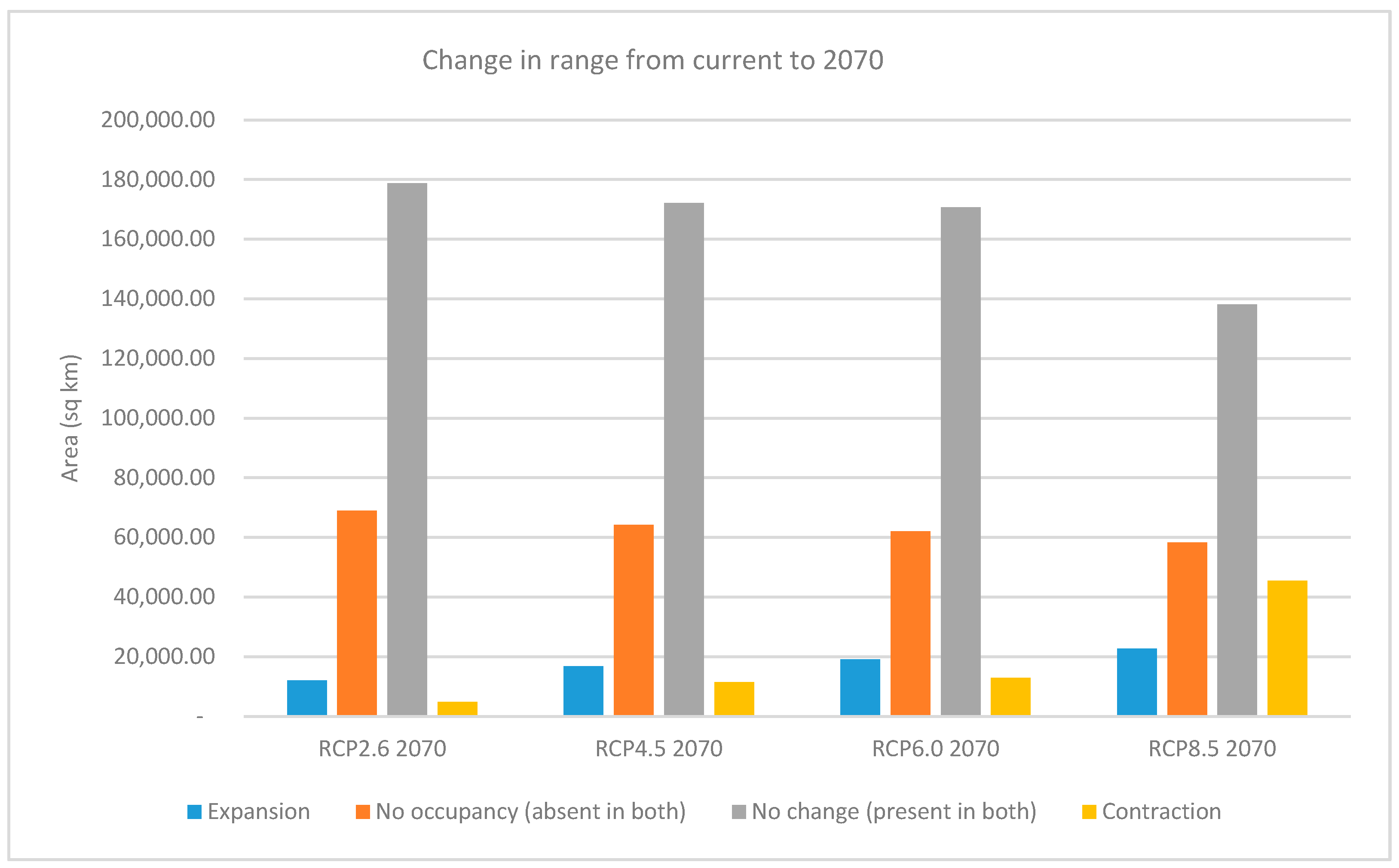
When the change in range characteristics of the thresholded presence/absence maps is calculated between current conditions and the RCP rasters for 2070, the contraction of the areas of species range is less than the area expansion, except for RCP8.5, where the opposite is true. The increase in the expansion range is shown to be directly proportional with increasing RCP values, with RCP8.5 showing an expansion in range almost double that of RCP2.6 (22,749 km2 vs. 12,089 km2). On the other hand, the areas that contract in RCP8.5 are much greater than the other scenarios combined. There is also a decrease in areas that show no change or presence in both rasters with the higher RCP values (Figure 7 and Table S1).
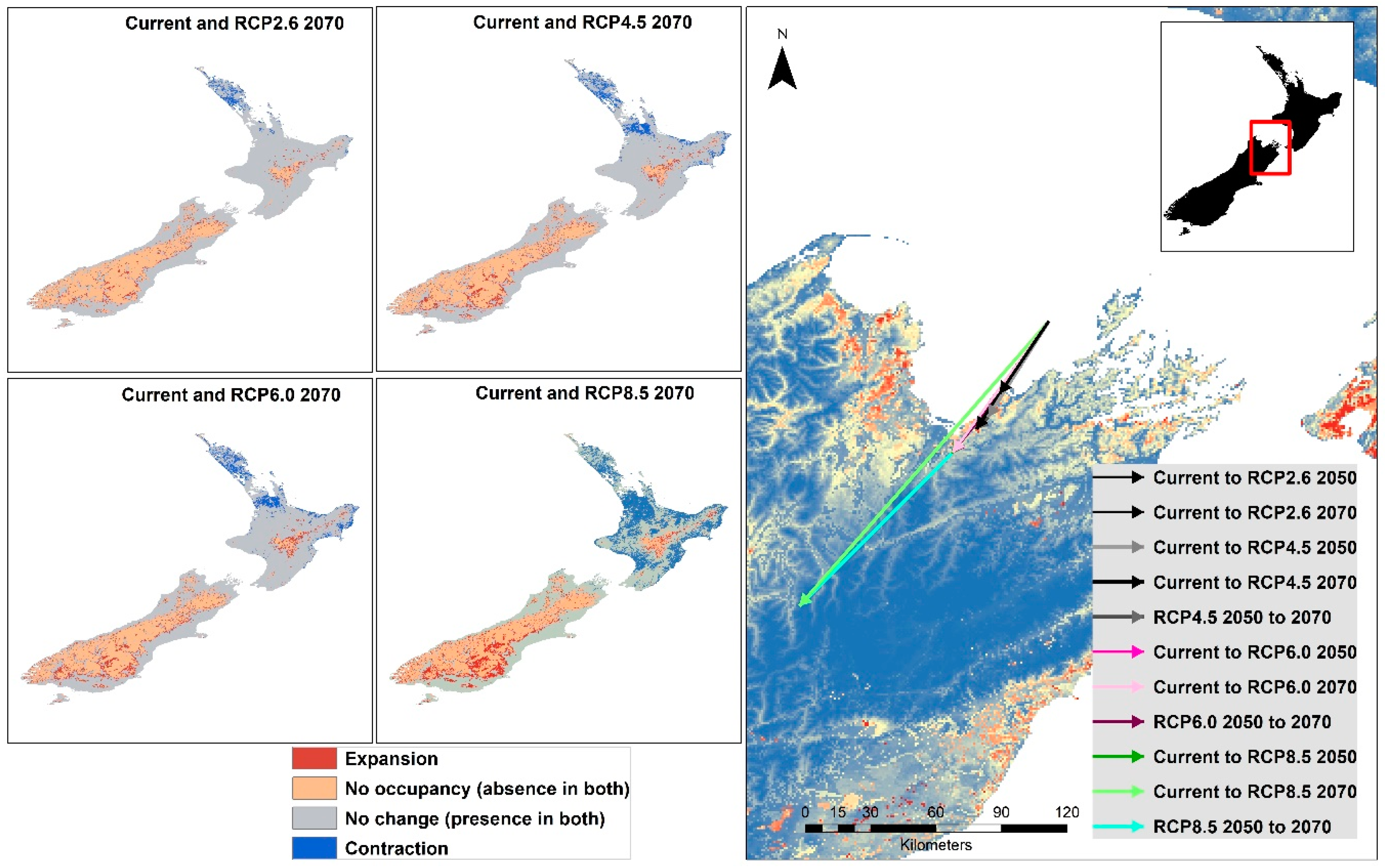
The range maps resulting from subtracting the thresholded future raster from the current raster show that North Island becomes less favorable for the Mexican daisy by the year 2070 for all RCP trajectories. An obvious range expansion in South Island is evident with increasing RCP values [77]. When centroid shifts were determined between the current and future as well as from 2050 to 2070 thresholded rasters, all shifts showed a movement and direction to the southwest, mainly along the length of New Zealand’s longitudinal axis (Figure 8). The magnitude of the centroid shift is also greater with higher RCP values, with RCP8.5 showing the highest magnitude. Centroid shifts for RCP4.5 is greater than RCP2.6, with the year-current-to-2070 shift greater than the shift from current to 2050. (Figure 8). When the range shift was calculated using the movement of the centroid, the values in were 0.57 km/year (RCP2.6), 0.85 km/year (RCP4.5), 1.06 km/year (RCP6.0) and 1.41 km/year (RCP8.5). The range of this movement is greater than the post-glacial migration rate of 140 plants estimated at values from 0.01 to 0.44 km/year, with a mean of 0.12 km/year [78].
4. Discussion
This work produced maps depicting spatial distribution and potential suitability of the Mexican daisy at global and New Zealand scales. The global maps show the widespread distribution of the Mexican daisy at its native and invaded areas. Regions with similar temperatures to its native range and coastal areas consistently show higher levels of suitability for the species. At a global scale, New Zealand shows very high levels of suitability and predicted presence/absence for the species. The species appears to be most prevalent in coastal regions; in addition to most of New Zealand it can also be seen along the southern coast of Australia, South America, Japan, and some areas in Europe. There are a few outliers where the species has been noted growing further inland, such as Africa and China. Outside of its native range, Optimized Hot Spot Analysis as well as CLOA show that New Zealand is the only country in the world with significant hotspots and significant outliers, a result that may be due to the number of occurrences reported in GBIF and that could indicate an inherent spatial bias due to uneven reporting [79]. This is also consistent with the country’s top 2 ranking in the number of invasive species recorded [80].
Recognized qualifications relevant in the use of SDM [81,82] related to this effort include the nature of occurrence data sourced from GBIF, use of a single performance metric in model evaluation and model parameters that may need iterative values to produce better results. In the absence of any other source of georeferenced location data, the rarefication and data processing conducted may also be considered as a form of subsampling that preserves the extent and contribution towards better predictive model [79] and removes some of the effects of sampling bias [83] because the source data is sufficiently large [81]. Further work to improve this aspect of modeling is certainly warranted. Using other evaluation metrics such as True Skills Statistics (TSS) and kappa [39,62] should increase confidence in the selection of models. For the model parameters specifically on threshold choice, related studies testing different threshold values derived from several model parameters such as sensitivity and specificity show more superior threshold options than the one used in this study [84,85]. Other threshold options, such as the maximum sum of sensitivity and specificity, that were shown to perform better [86,87] could therefore be tested and compared for use in future iterations of the species distribution modeling for the Mexican daisy.
Looking at the relationship between the distribution of the species at both global and New Zealand scales can assist in managing the spread of the species within New Zealand. Currently the Mexican daisy is growing in many major regions across the globe and New Zealand, most notably around the major urban centers Auckland, Wellington, Christchurch and coastal regions of South Island. This is consistent with the characteristic of the Mexican daisy in forest areas to be associated with the size and proximity of settlements [18]. The modeling results provide information for conservation and management planning for areas of considerable importance most likely to be impacted by the spread and establishment of the species. The information inherent in the maps showing the geographical distribution and results of the geostatistical processing in ArcMap as well as SDM provides graphical knowledge contributing to the effectiveness of related control measures by providing a guide to areas for focusing resources or prioritizing mitigation or eradication measures that are required [88]. Regions with the higher current density show changes in suitability under future climatic conditions. Further exploration of other environmental and even socio-economic characteristics in areas such as Auckland, Wellington and South Island will refine the model and contribute to an increased understanding of the species’ ability to establish, grow and spread successfully in these regions. The spread into southern regions in New Zealand is of concern especially in novel areas where native plants are at risk from the competition of the species invading its ecological niche and other associated impacts on the conservation of biodiversity for New Zealand in general. The decrease in habitat suitability overall is consistent with modeling work on invasive species in Australia that compares current and future conditions of hundreds of invasive plants [89].
There is evidence that the species will increase its range in South Island, as well as regions in the south of North Island. This is consistent with the report in the Himalayas that include the Mexican daisy among 11 invasive species modeled similarly and depicting that such will spread to higher elevation and latitudes with global warming [39]. Species distribution modeling predicts that the Mexican Daisy will spread to other areas where it may not currently be a concern under conditions of increasing greenhouse gas emissions.
This information will allow managers of those areas becoming more suitable, particularly in the southern areas of the country, to prioritize or increase the risk rating of the Mexican daisy for their respective regions. Conversely, in areas where the model shows a contraction of range, less focus on the species would reduce its risk rating, providing information for allocating resources to other more risky plants or organisms [90].
5. Conclusions
The results of this work provide an overview of the potential impacts and spread of the Mexican daisy in New Zealand. The combination of geostatistical processing and SDM provided several predictive maps that can be used to assesses measures for controlling the species. The resulting maps provided clear indications where the species will most likely spread over the next several years, primarily because of changing and warming climate regime as represented in the environmental variables used. This provides a basis and starting point from which to formulate a management plan and also point out for the need for additional research work, including enhancing the data needed for more robust and relevant modeling.
Supplementary Materials
The following are available online at https://0-www-mdpi-com.brum.beds.ac.uk/2225-1154/7/2/24/s1, Table S1: Calculated changes in expansion/contraction of the species in New Zealand.
Author Contributions
Data curation, L.H.; Formal analysis, L.H and G.A; Funding acquisition, D.B; Investigation, L.H; Methodology, L.H. and G.A.; Project administration, D.B; Resources, D.B; Software, L.H; Supervision, G.A; Writing—original draft, L.H; Writing—review and editing, G.A and D.B.
Funding
This research was funded by the Auckland Council.
Acknowledgments
The authors would like to thank the Auckland Council for funding and supporting this project and Unitec Institute of Technology for the computing facilities used in processing the data.
Conflicts of Interest
The authors declare no conflict of interest
References
- Hind, N. 729. ERIGERON KARVINSKIANUS. Curtis’s Bot. Mag. 2012, 29, 52–65. [Google Scholar] [CrossRef]
- Bala, S.; Kaushal, B.; Goyal, H.; Gupta, R.C. A Case of Synaptic Mutant in Erigeron Karvinskianus DC. (Latin American Fleabane). Cytologia 2010, 75, 299–304. [Google Scholar] [CrossRef]
- Henderson, L. Mapping of Invasive Alien Plants: The Contribution of the Southern African Plant Invaders Atlas (SAPIA) to Biological Weed Control. Afr. Entomol. 2011, 19, 498–503. [Google Scholar] [CrossRef]
- Hussey, B.M.J.; Keighery, G.J.; Cousens, R.D.; Dodd, J.; Lloyd, S.G. Western Weeds: A Guide to the Weeds of Western Australia (The Plant Protection Society of Western Australia (Inc.): Perth). Available online: https://www.wswa.org.au/western_weeds.htm#contents (accessed on 1 July 2018).
- Mito, T.; Uesugi, T. Invasive Alien Species in Japan: The Status Quo and the New Regulation for Prevention of Their Adverse Effects. Glob. Environ. Res. 2004, 8, 171–191. [Google Scholar]
- Negi, P.S.; Hajra, P.K. Alien Flora of Doon Valley, Northwest Himalaya. Curr. Sci. 2007, 92, 968–978. [Google Scholar]
- Botella, C.; Joly, A.; Bonnet, P.; Monestiez, P.; Munoz, F. Species Distribution Modeling Based on the Automated Identification of Citizen Observations. Appl. Plant Sci. 2018, 6, e1029. [Google Scholar] [CrossRef] [PubMed]
- Celesti-Grapow, L.; Blasi, C. The Role of Alien and Native Weeds in the Deterioration of Archaeological Remains in Italy. Weed Technol. 2004, 1508–1513. [Google Scholar]
- Lorence, D.H.; Perlman, S. A New Species of Cyrtandra (Gesneriaceae) from Hawai ‘i, Hawaiian Islands. Novon A J. Bot. Nomencl. 2007, 17, 357–361. [Google Scholar] [CrossRef]
- Wood, K.R. Rediscovery, Conservation Status and Taxonomic Assessment of Melicope Degeneri (Rutaceae), Kaua ‘i, Hawai ‘I. Endanger. Species Res. 2011, 14, 61–68. [Google Scholar] [CrossRef]
- Baret, S.; Rouget, M.; Richardson, D.M.; Lavergne, C.; Egoh, B.; Dupont, J.; Strasberg, D. Current Distribution and Potential Extent of the Most Invasive Alien Plant Species on La Réunion (Indian Ocean, Mascarene Islands). Austral Ecol. 2006, 31, 747–758. [Google Scholar] [CrossRef]
- Webb, C.J. Checklist of Dicotyledons Naturalised in New Zealand 18. Asteraceae (Compositae) Subfamily Asteroideae. N. Z. J. Bot. 1987, 25, 489–501. [Google Scholar] [CrossRef]
- Given, D.R. Checklist of Dicotyledons Naturalised in New Zealand 16. Compositae—Tribes Vernonieae, Eupatorieae, Astereae, Inuleae, Heliantheae, Tageteae, Calenduleae, and Arctoteae. N. Z. J. Bot. 1984, 22, 183–190. [Google Scholar] [CrossRef]
- Heenan, P.B.; De Lange, P.J.; Rance, B.D.; Sykes, W.R.; Meurk, C.D.; Korver, M.A. Additional Records of Indigenous and Naturalised Plants with Observations on the Distribution of Gunnera Tinctoria, on Stewart Island, New Zealand. N. Z. J. Bot. 2009, 47, 1–7. [Google Scholar] [CrossRef]
- Esler, A.E. The Naturalisation of Plants in Urban Auckland, New Zealand 3. Catalogue of Naturalised Species. N. Z. J. Bot. 1987, 25, 539–558. [Google Scholar] [CrossRef]
- Cameron, E.K. Environmental Vascular Plant Weeds and New Records for Motutapu, Waitemata Harbour. Auckl. Bot. Soc. J. 1994, 49, 3340. [Google Scholar]
- Wilcox, M.D.; Rogan, D.B. The Mural Flora of Auckland. Auckl. Bot. Soc. J. 1999, 54, 35–46. [Google Scholar]
- Sullivan, J.J.; Timmins, S.M.; Williams, P.A. Movement of Exotic Plants into Coastal Native Forests from Gardens in Northern New Zealand. N. Z. J. Ecol. 2005, 29, 1–10. [Google Scholar]
- Barton, J.; Fowler, S.V.; Gianotti, A.F.; Winks, C.J.; De Beurs, M.; Arnold, G.C.; Forrester, G. Successful Biological Control of Mist Flower (Ageratina Riparia) in New Zealand: Agent Establishment, Impact and Benefits to the Native Flora. Biol. Control 2007, 40, 370–385. [Google Scholar] [CrossRef]
- Clout, M.N.; Lowe, S.J. Invasive Species and Environmental Changes in New Zealand. In Invasive Species in a Changing World; Mooney, H., Hobbs, R., Eds.; Island Press Washington, District of Columbia: Washington, DC, USA, 2000. [Google Scholar]
- Appendix One: Invasive Weeds in the “Protecting and Restoring our Natural Heritage—A Practical Guide”. Available online: https://www.doc.govt.nz/about-us/science-publications/conservation-publications/protecting-and-restoring-our-natural-heritage-a-practical-guide/appendix-one-invasive-weeds (accessed on 28 November 2018).
- Appendix One: Invasive Weeds in the “Protecting and Restoring our Natural Heritage—A Practical Guide”. Available online: https://www.doc.govt.nz/documents/conservation/native-plants/motukarara-nursery/restoration-guide-complete.pdf (accessed on 28 November 2018).
- Williams, J.A.; West, C.J. Environmental Weeds in Australia and New Zealand: Issues and Approaches to Management. Austral Ecol. 2000, 25, 425–444. [Google Scholar] [CrossRef]
- Biosecurity New Zealand. Mexican Daisy. Available online: https://www.mpi.govt.nz/protection-and-response/finding-and-reporting-pests-and-diseases/pest-and-disease-search?Customisnppa=1 (accessed on 28 November 2018).
- Auckland Council. Surveillance Pest Plants, Auckland Regional Pest Strategy 2007–2012. Available online: https://www.aucklandcouncil.govt.nz/plans-projects-policies-reports-bylaws/our-plans-strategies/topic-based-plans-strategies/environmental-plans-strategies/docsregionalpestmanagementstrategy/surveillance-pest-plants-part-1.pdf (accessed on 28 November 2018).
- Pitelka, L.F.; Workshop, M. Plant Migration and Climate Change. Am. Sci. 2014, 85, 464–473. [Google Scholar]
- Meyerson, L.A.; Mooney, H.A. Invasive Alien Species in an Era of Globalization. Front. Ecol. Environ. 2007, 5, 199–208. [Google Scholar] [CrossRef]
- Thomas, Z.A.; Turney, C.S.M.; Palmer, J.G.; Lloydd, S.; Klaricich, J.N.L.; Hogg, A. Extending the Observational Record to Provide New Insights into Invasive Alien Species in a Coastal Dune Environment of New Zealand. Appl. Geogr. 2018, 98, 100–109. [Google Scholar] [CrossRef]
- Weber, E.; Gut, D. Assessing the Risk of Potentially Invasive Plant Species in Central Europe. J. Nat. Conserv. 2004, 12, 171–179. [Google Scholar] [CrossRef]
- O’Donnell, J.; Gallagher, R.V.; Wilson, P.D.; Downey, P.O.; Hughes, L.; Leishman, M.R. Invasion Hotspots for Non-Native Plants in Australia under Current and Future Climates. Glob. Chang. Biol. 2012, 18, 617–629. [Google Scholar] [CrossRef]
- Peterson, A.T.; Nakazawa, Y. Environmental Data Sets Matter in Ecological Niche Modelling: An Example with Solenopsis Invicta and Solenopsis Richteri. Glob. Ecol. Biogeogr. 2008, 17, 135–144. [Google Scholar] [CrossRef]
- Kulhanek, S.A.; Leung, B.; Ricciardi, A. Using Ecological Niche Models to Predict the Abundance and Impact of Invasive Species: Application to the Common Carp. Ecol. Appl. 2011, 21, 203–213. [Google Scholar] [CrossRef] [PubMed]
- Fraser, D.; Aguilar, G.; Nagle, W.; Galbraith, M.; Ryall, C. The House Crow (Corvus Splendens): A Threat to New Zealand? ISPRS Int. J. Geo-Inf. 2015, 4, 725–740. [Google Scholar] [CrossRef]
- Yang, X.-Q.; Kushwaha, S.P.S.; Saran, S.; Xu, J.; Roy, P.S. Maxent Modeling for Predicting the Potential Distribution of Medicinal Plant, Justicia Adhatoda L. in Lesser Himalayan Foothills. Ecol. Eng. 2013, 51, 83–87. [Google Scholar] [CrossRef]
- Pěknicová, J.; Berchová-Bímová, K. Application of Species Distribution Models for Protected Areas Threatened by Invasive Plants. J. Nat. Conserv. 2016, 34, 1–7. [Google Scholar] [CrossRef]
- Yost, A.C.; Petersen, S.L.; Gregg, M.; Miller, R. Predictive Modeling and Mapping Sage Grouse (Centrocercus Urophasianus) Nesting Habitat Using Maximum Entropy and a Long-Term Dataset from Southern Oregon. Ecol. Inform. 2008, 3, 375–386. [Google Scholar] [CrossRef]
- Chai, S.-L.; Zhang, J.; Nixon, A.; Nielsen, S. Using Risk Assessment and Habitat Suitability Models to Prioritise Invasive Species for Management in a Changing Climate. PLoS ONE 2016, 11, e0165292. [Google Scholar] [CrossRef] [PubMed]
- Taylor, S.; Kumar, L. Potential Distribution of an Invasive Species under Climate Change Scenarios Using CLIMEX and Soil Drainage: A Case Study of Lantana Camara L. in Queensland, Australia. J. Environ. Manag. 2013, 114, 414–422. [Google Scholar] [CrossRef]
- Aguilar, G.D.; Blanchon, D.J.; Foote, H.; Pollonais, C.W.; Mosee, A.N. A Performance Based Consensus Approach for Predicting Spatial Extent of the Chinese Windmill Palm (Trachycarpus Fortunei) in New Zealand under Climate Change. Ecol. Inform. 2017, 39, 130–139. [Google Scholar] [CrossRef]
- Anderson, R.P.; Araújo, M.B.; Guisan, A.; Lobo, J.M.; Martínez-Meyer, E.; Peterson, A.T.; Soberón, J. Final Report of the Task Group on GBIF Data Fitness for Use in Distribution Modelling. 2016. Available online: https://0-doi-org.brum.beds.ac.uk/10.13140/RG.2.2.27191.93608 (accessed on 28 November 2018).
- ESRI. Arcmap. Available online: http://desktop.arcgis.com/en/arcmap/ (accessed on 12 November 2018).
- ESRI. Kernel Density. Available online: http://desktop.arcgis.com/en/arcmap/10.5/tools/spatial-analyst-toolbox/kernel-density.htm (accessed on 12 November 2018).
- Getis, A.; Ord, J.K. The Analysis of Spatial Association by Use of Distance Statistics. In Perspectives on Spatial Data Analysis; Springer: Berlin, Germany, 2010; pp. 127–145. [Google Scholar]
- Ord, J.K.; Getis, A. Local Spatial Autocorrelation Statistics: Distributional Issues and an Application. Geogr. Anal. 1995, 27, 286–306. [Google Scholar] [CrossRef]
- ESRI. How Hot Spot Analysis (Getis-Ord Gi*) Works. Available online: http://pro.arcgis.com/en/pro-app/tool-reference/spatial-statistics/h-how-hot-spot-analysis-getis-ord-gi-spatial-stati.htm (accessed on 9 November 2018).
- Anselin, L. Local Indicators of Spatial Association—LISA. Geogr. Anal. 1995, 27, 93–115. [Google Scholar] [CrossRef]
- ESRI. How Cluster and Outlier Analysis (Anselin Local Moran’s I) Works. Available online: http://pro.arcgis.com/en/pro-app/tool-reference/spatial-statistics/h-how-cluster-and-outlier-analysis-anselin-local-m.htm (accessed on 12 November 2018).
- Baldwin, R. Use of Maximum Entropy Modeling in Wildlife Research. Entropy 2009, 11, 854–866. [Google Scholar] [CrossRef] [Green Version]
- Fourcade, Y.; Engler, J.O.; Rödder, D.; Secondi, J. Mapping Species Distributions with MAXENT Using a Geographically Biased Sample of Presence Data: A Performance Assessment of Methods for Correcting Sampling Bias. PLoS ONE 2014, 9, e97122. [Google Scholar] [CrossRef] [PubMed]
- Phillips, S.J.; Anderson, R.P.; Schapire, R.E. Maximum Entropy Modeling of Species Geographic Distributions. Ecol. Model. 2006, 190, 231–259. [Google Scholar] [CrossRef]
- Elith, J.; Leathwick, J.R. Species Distribution Models: Ecological Explanation and Prediction Across Space and Time. Annu. Rev. Ecol. Evol. Syst. 2009, 40, 677–697. [Google Scholar] [CrossRef]
- Phillips, S.J.; Dudík, M.; Elith, J.; Graham, C.H.; Lehmann, A.; Leathwick, J.; Ferrier, S. Sample Selection Bias and Presence-only Distribution Models: Implications for Background and Pseudo-absence Data. Ecol. Appl. 2009, 19, 181–197. [Google Scholar] [CrossRef]
- Wan, J.Z.; Wang, C.J.; Yu, F.H. Impacts of the Spatial Scale of Climate Data on the Modeled Distribution Probabilities of Invasive Tree Species throughout the World. Ecol. Inform. 2016, 36, 42–49. [Google Scholar] [CrossRef]
- Jaryan, V.; Datta, A.; Uniyal, S.K.; Kumar, A.; Gupta, R.C.; Singh, R.D. Modelling Potential Distribution of Sapium Sebiferum—An Invasive Tree Species in Western Himalaya. Curr. Sci. 2013, 105, 1282–1287. [Google Scholar] [CrossRef]
- Hijmans, R.J.; Cameron, S.E.; Parra, J.L.; Jones, P.G.; Jarvis, A. Very High Resolution Interpolated Climate Surfaces for Global Land Areas. Int. J. Climatol. 2005, 25, 1965–1978. [Google Scholar] [CrossRef]
- Aguilar, G.D.; Farnworth, M.J.; Winder, L. Mapping the Stray Domestic Cat (Felis Catus) Population in New Zealand: Species Distribution Modelling with a Climate Change Scenario and Implications for Protected Areas. Appl. Geogr. 2015, 63, 146–154. [Google Scholar] [CrossRef]
- Khanum, R.; Mumtaz, A.S.; Kumar, S. Predicting Impacts of Climate Change on Medicinal Asclepiads of Pakistan Using Maxent Modeling. Acta Oecol. 2013, 49, 23–31. [Google Scholar] [CrossRef]
- Hufnagel, L.; Garamvölgyi, Á. Impacts of Climate Change on Vegetation Distribution. No. 1: Climate Change Induced Vegetation Shifts in the Palearctic Region. Appl. Ecol. Environ. Res. 2013, 11, 79–122. [Google Scholar]
- Carraro, C.; Lanza, A.; Tavoni, M. All You Need to Know About the IPCC 5th Assessment Report. Mitigation of Climate Change. Rev. Environ. Energy Econ. 2014. [Google Scholar]
- Brown, J.L. SDMtoolbox: A Python-Based GIS Toolkit for Landscape Genetic, Biogeographic and Species Distribution Model Analyses. Methods Ecol. Evol. 2014, 5, 694–700. [Google Scholar] [CrossRef]
- Miller, J.A. Species Distribution Models: Spatial Autocorrelation and Non-Stationarity. Prog. Phys. Geogr. 2012, 36, 681–692. [Google Scholar] [CrossRef]
- De Oliveira, G.; Rangel, T.F.; Lima-Ribeiro, M.S.; Terribile, L.C.; Diniz-Filho, J.A.F. Evaluating, Partitioning, and Mapping the Spatial Autocorrelation Component in Ecological Niche Modeling: A New Approach Based on Environmentally Equidistant Records. Ecography 2014, 37, 637–647. [Google Scholar] [CrossRef]
- Tsoar, A.; Allouche, O.; Steinitz, O.; Rotem, D.; Kadmon, R. A Comparative Evaluation of Presence-Only Methods for Modelling Species Distribution. Divers. Distrib. 2007, 13, 397–405. [Google Scholar] [CrossRef]
- Wisz, M.S.; Hijmans, R.J.; Li, J.; Peterson, A.T.; Graham, C.H.; Guisan, A. Effects of Sample Size on the Performance of Species Distribution Models. Divers. Distrib. 2008, 14, 763–773. [Google Scholar] [CrossRef]
- Nagaraju, S.K.; Gudasalamani, R.; Barve, N.; Ghazoul, J.; Narayanagowda, G.K.; Ramanan, U.S. Do Ecological Niche Model Predictions Reflect the Adaptive Landscape of Species? A Test Using Myristica Malabarica Lam., an Endemic Tree in the Western Ghats, India. PLoS ONE 2013, 8, e82066. [Google Scholar] [CrossRef] [PubMed]
- Khadka, K.K.; James, D.A. Modeling and Mapping the Current and Future Climatic-Niche of Endangered Himalayan Musk Deer. Ecol. Inform. 2017, 40, 1–7. [Google Scholar] [CrossRef]
- Pearson, R.G.; Raxworthy, C.J.; Nakamura, M.; Townsend Peterson, A. Predicting Species Distributions from Small Numbers of Occurrence Records: A Test Case Using Cryptic Geckos in Madagascar. J. Biogeogr. 2006, 34, 102–117. [Google Scholar] [CrossRef]
- Thorn, J.S.; Nijman, V.; Smith, D.; Nekaris, K.A.I. Ecological Niche Modelling as a Technique for Assessing Threats and Setting Conservation Priorities for Asian Slow Lorises (Primates: Nycticebus). Divers. Distrib. 2009, 15, 289–298. [Google Scholar] [CrossRef]
- Raxworthy, C.J.; Ingram, C.M.; Rabibisoa, N.; Pearson, R.G. Applications of Ecological Niche Modeling for Species Delimitation: A Review and Empirical Evaluation Using Day Geckos (Phelsuma) from Madagascar. Syst. Biol. 2007, 56, 907–923. [Google Scholar] [CrossRef] [Green Version]
- Sellers, P.J.; Mintz, Y.; Sud, Y.E.A.; Dalcher, A. A Simple Biosphere Model (SiB) for Use within General Circulation Models. J. Atmos. Sci. 1986, 43, 505–531. [Google Scholar] [CrossRef]
- Loveland, T.R.; Reed, B.C.; Brown, J.F.; Ohlen, D.O.; Zhu, Z.; Yang, L.; Merchant, J.W. Development of a Global Land Cover Characteristics Database and IGBP DISCover from 1 Km AVHRR Data. Int. J. Remote Sens. 2000, 21, 1303–1330. [Google Scholar] [CrossRef]
- Petitpierre, B.; McDougall, K.; Seipel, T.; Broennimann, O.; Guisan, A.; Kueffer, C. Will Climate Change Increase the Risk of Plant Invasions into Mountains? Ecol. Appl. 2016, 26, 530–544. [Google Scholar] [CrossRef]
- Dormann, C.F.; Elith, J.; Bacher, S.; Buchmann, C.; Carl, G.; Carré, G.; Marquéz, J.R.G.; Gruber, B.; Lafourcade, B.; Leitão, P.J. Collinearity: A Review of Methods to Deal with It and a Simulation Study Evaluating Their Performance. Ecography 2013, 36, 27–46. [Google Scholar] [CrossRef]
- Raxworthy, C.J.; Martinez-Meyer, E.; Horning, N.; Nussbaum, R.A.; Schneider, G.E.; Ortega-Huerta, M.A.; Peterson, A.T. Predicting Distributions of Known and Unknown Reptile Species in Madagascar. Nature 2003, 426, 837–841. [Google Scholar] [CrossRef] [PubMed]
- Rödder, D.; Lötters, S. Niche Shift versus Niche Conservatism? Climatic Characteristics of the Native and Invasive Ranges of the Mediterranean House Gecko (Hemidactylus Turcicus). Glob. Ecol. Biogeogr. 2009, 18, 674–687. [Google Scholar] [CrossRef]
- Hanberry, B.B.; He, H.S. Prevalence, Statistical Thresholds, and Accuracy Assessment for Species Distribution Models. Web Ecol. 2013, 13, 13–19. [Google Scholar] [CrossRef]
- Thapa, S.; Chitale, V.; Rijal, S.J.; Bisht, N.; Shrestha, B.B. Understanding the Dynamics in Distribution of Invasive Alien Plant Species under Predicted Climate Change in Western Himalaya. PLoS ONE 2018. [Google Scholar] [CrossRef] [PubMed]
- Cunze, S.; Heydel, F.; Tackenberg, O. Are Plant Species Able to Keep Pace with the Rapidly Changing Climate? PLoS ONE 2013, 8. [Google Scholar] [CrossRef] [PubMed]
- Beck, J.; Böller, M.; Erhardt, A.; Schwanghart, W. Spatial Bias in the GBIF Database and Its Effect on Modeling Species’ Geographic Distributions. Ecol. Inform. 2014, 19, 10–15. [Google Scholar] [CrossRef]
- Turbelin, A.J.; Malamud, B.D.; Francis, R.A. Mapping the Global State of Invasive Alien Species: Patterns of Invasion and Policy Responses. Glob. Ecol. Biogeogr. 2017, 26, 78–92. [Google Scholar] [CrossRef]
- Araújo, M.B.; Guisan, A. Five (or so) Challenges for Species Distribution Modelling. J. Biogeogr. 2006, 33, 1677–1688. [Google Scholar] [CrossRef]
- Narouei-Khandan, H.A.; Halbert, S.E.; Worner, S.P.; van Bruggen, A.H.C. Global Climate Suitability of Citrus Huanglongbing and Its Vector, the Asian Citrus Psyllid, Using Two Correlative Species Distribution Modeling Approaches, with Emphasis on the USA. Eur. J. Plant Pathol. 2016, 144, 655–670. [Google Scholar] [CrossRef]
- Engemann, K.; Enquist, B.J.; Sandel, B.; Boyle, B.; Jørgensen, P.M.; Morueta-Holme, N.; Peet, R.K.; Violle, C.; Svenning, J.C. Limited Sampling Hampers “Big Data” Estimation of Species Richness in a Tropical Biodiversity Hotspot. Ecol. Evol. 2015, 5, 807–820. [Google Scholar] [CrossRef] [PubMed]
- Liu, C.; Newell, G.; White, M. On the Selection of Thresholds for Predicting Species Occurrence with Presence-Only Data. Ecol. Evol. 2016, 6, 337–348. [Google Scholar] [CrossRef] [PubMed]
- Bean, W.T.; Stafford, R.; Brashares, J.S. The Effects of Small Sample Size and Sample Bias on Threshold Selection and Accuracy Assessment of Species Distribution Models. Ecography 2012, 35, 250–258. [Google Scholar] [CrossRef]
- Liu, C.; White, M.; Newell, G. Selecting Thresholds for the Prediction of Species Occurrence with Presence-only Data. J. Biogeogr. 2013, 40, 778–789. [Google Scholar] [CrossRef]
- Rota, C.T.; Fletcher, R.J.; Evans, J.M.; Hutto, R.L. Does Accounting for Imperfect Detection Improve Species Distribution Models? Ecography 2011, 34, 659–670. [Google Scholar] [CrossRef]
- Uden, D.R.; Allen, C.R.; Angeler, D.G.; Corral, L.; Fricke, K.A. Adaptive Invasive Species Distribution Models: A Framework for Modeling Incipient Invasions. Biol. Invasions 2015, 17, 2831–2850. [Google Scholar] [CrossRef]
- Roger, E.; Duursma, D.E.; Downey, P.O.; Gallagher, R.V.; Hughes, L.; Steel, J.; Johnson, S.B.; Leishman, M.R. A Tool to Assess Potential for Alien Plant Establishment and Expansion under Climate Change. J. Environ. Manag. 2015, 159, 121–127. [Google Scholar] [CrossRef]
- Jarnevich, C.S.; Stohlgren, T.J. Near Term Climate Projections for Invasive Species Distributions. Biol. Invasions 2009, 11, 1373–1379. [Google Scholar] [CrossRef]
Figure 1.
Worldwide occurrence of the Mexican daisy, using Hotspot and Cluster and Outlier Analysis.
Figure 1.
Worldwide occurrence of the Mexican daisy, using Hotspot and Cluster and Outlier Analysis.

Figure 2.
New Zealand occurrences, kernel density surface, Hotspot, and Cluster and Outlier Analysis maps.
Figure 2.
New Zealand occurrences, kernel density surface, Hotspot, and Cluster and Outlier Analysis maps.

Figure 3.
Occurrences, Hotspots and CLOA maps for Auckland.

Figure 4.
Results of suitability mapping and prediction of presence absence using Maxent for the 100 km rarefied occurrence data and non-correlated variables.
Figure 4.
Results of suitability mapping and prediction of presence absence using Maxent for the 100 km rarefied occurrence data and non-correlated variables.

Figure 5.
New Zealand suitability for the Mexican daisy under different climate scenarios and years.
Figure 5.
New Zealand suitability for the Mexican daisy under different climate scenarios and years.

Figure 6.
New Zealand presence and absence threshold for the Mexican daisy under different climate scenarios and years.
Figure 6.
New Zealand presence and absence threshold for the Mexican daisy under different climate scenarios and years.

Figure 7.
Prediction of range expansion and contraction for the Representative Concentration Pathways (RCPs) in 2070.
Figure 7.
Prediction of range expansion and contraction for the Representative Concentration Pathways (RCPs) in 2070.

Figure 8.
Changes in range of the Mexican daisy from current to 2070 under different RCP trajectories and shift of centroids of the thresholded rasters.
Figure 8.
Changes in range of the Mexican daisy from current to 2070 under different RCP trajectories and shift of centroids of the thresholded rasters.


Table 1.
Area under the curve (AUC) values of different rarefication values for worldwide and New Zealand Erigeron species distribution to identify correlated environmental variables.
Table 1.
Area under the curve (AUC) values of different rarefication values for worldwide and New Zealand Erigeron species distribution to identify correlated environmental variables.
| Distance (km) | World | NZ | ||
|---|---|---|---|---|
| No. of Samples | AUC | No. of Samples | AUC | |
| 1 | 3564 | 0.919 | 216 | 0.915 |
| 5 | 1232 | 0.934 | 127 | 0.914 |
| 10 | 1147 | 0.927 | 97 | 0.896 |
| 20 | 867 | 0.937 | 74 | 0.860 |
| 50 | 467 | 0.947 | 46 | 0.832 |
| 100 | 274 | 0.951 | 28 | 0.821 |
Table 2.
Values of Bioclim measured at the occurrence points.
| Layer | Climatic Variable | Minimum | Maximum | Mean | Standard Error | Standard Deviation |
|---|---|---|---|---|---|---|
| *BIO1 | Annual Mean Temperature | 1.594 | 27.354 | 13.991 | 0.160 | 4.125 |
| *BIO2 | Mean Diurnal Range (Mean of monthly (max temperature–min temperature)) | 4.863 | 18.540 | 9.700 | 0.102 | 2.634 |
| BIO3 | Isothermality (BIO2/BIO7) (* 100) | 0.239 | 0.913 | 0.482 | 0.006 | 0.152 |
| BIO4 | Temperature Seasonality (standard deviation * 100) | 0.001 | 0.029 | 0.013 | 0.000 | 0.006 |
| BIO5 | Max Temperature of Warmest Month | 13.400 | 37.236 | 24.955 | 0.151 | 3.906 |
| BIO6 | Min Temperature of Coldest Month | −9.371 | 19.048 | 4.138 | 0.182 | 4.702 |
| BIO7 | Temperature Annual Range (BIO5–BIO6) | 8.587 | 35.222 | 20.809 | 0.165 | 4.270 |
| BIO8 | Mean Temperature of Wettest Quarter | −3.399 | 29.053 | 13.334 | 0.227 | 5.867 |
| BIO9 | Mean Temperature of Driest Quarter | −5.387 | 26.571 | 14.703 | 0.230 | 5.936 |
| BIO10 | Mean Temperature of Warmest Quarter | 8.780 | 29.130 | 18.830 | 0.128 | 3.291 |
| BIO11 | Mean Temperature of Coldest Quarter | −5.392 | 26.286 | 9.213 | 0.217 | 5.604 |
| *BIO12 | Annual Precipitation | 134.000 | 4330.000 | 1102.018 | 21.867 | 564.320 |
| BIO13 | Precipitation of Wettest Month | 6.894 | 169.847 | 36.987 | 0.946 | 24.404 |
| BIO14 | Precipitation of Driest Month | 0.000 | 64.178 | 9.243 | 0.269 | 6.938 |
| *BIO15 | Precipitation Seasonality (Coefficient of Variation) | 0.067 | 1.258 | 0.411 | 0.011 | 0.284 |
| BIO16 | Precipitation of Wettest Quarter | 78.355 | 1852.770 | 431.371 | 10.458 | 269.901 |
| BIO17 | Precipitation of Driest Quarter | 0.629 | 949.616 | 142.521 | 3.829 | 98.828 |
| BIO18 | Precipitation of Warmest Quarter | 4.765 | 1278.280 | 268.646 | 7.392 | 190.758 |
| BIO19 | Precipitation of Coldest Quarter | 17.143 | 951.106 | 238.663 | 6.082 | 156.966 |
* used in the Maxent model.
Table 3.
Results of the jackknife of variable contributions and model response to the variables.
| Variable | Percent Contribution | Permutation Importance | Response of Model to Variable | |
|---|---|---|---|---|
| Model with all Variables | Model with Only the Corresponding Variable | |||
| Population | 46 | 10.5 |  |  |
| Land Cover | 22.7 | 26 |  |  |
| BIO1 | 17.3 | 35.9 |  |  |
| Elevation | 9.7 | 13.8 |  |  |
| BIO15 | 2.7 | 4.2 |  |  |
| BIO2 | 1.4 | 7.2 |  |  |
| BIO12 | 0.3 | 2.4 |  |  |
© 2019 by the authors. Licensee MDPI, Basel, Switzerland. This article is an open access article distributed under the terms and conditions of the Creative Commons Attribution (CC BY) license (http://creativecommons.org/licenses/by/4.0/).
Share and Cite
MDPI and ACS Style
Hannah, L.; Aguilar, G.; Blanchon, D. Spatial Distribution of the Mexican Daisy, Erigeron karvinskianus, in New Zealand under Climate Change. Climate 2019, 7, 24. https://0-doi-org.brum.beds.ac.uk/10.3390/cli7020024
AMA Style
Hannah L, Aguilar G, Blanchon D. Spatial Distribution of the Mexican Daisy, Erigeron karvinskianus, in New Zealand under Climate Change. Climate. 2019; 7(2):24. https://0-doi-org.brum.beds.ac.uk/10.3390/cli7020024
Chicago/Turabian StyleHannah, Lauren, Glenn Aguilar, and Dan Blanchon. 2019. "Spatial Distribution of the Mexican Daisy, Erigeron karvinskianus, in New Zealand under Climate Change" Climate 7, no. 2: 24. https://0-doi-org.brum.beds.ac.uk/10.3390/cli7020024
Note that from the first issue of 2016, this journal uses article numbers instead of page numbers. See further details here.