Adaptive Tracking Method for Non-Cooperative Continuously Thrusting Spacecraft

Abstract

Performance of the traditional Kalman filter and its variants can seriously degrade when they are used to track a non-cooperative continuously thrusting spacecraft. To overcome this shortcoming, an adaptive tracking method for relative state estimation of a non-cooperative target is proposed based on the interacting multiple model (IMM) algorithm. First, built upon a current statistical jerk (CSJerk) model, a robust CSJerk filtering (RCSJF) algorithm is developed, which can address the issue of low estimation accuracy and instability of traditional approaches at the moments when the spacecraft starts and ends thrusting. Second, the developed RCSJF algorithm is further used to form the model set of the IMM by incorporating different maximum jerk values, based on which an adaptive tracking method is presented that can track a non-cooperative target with different maneuvering levels. Simulation results show that the proposed method can effectively track the target across all thrusts levels under the conditions considered, and the convergence performance of the proposed method is improved in comparison to the CSJerk-based extended Kalman filter, especially at the start and end time of the maneuver.

1. Introduction

In cooperative space rendezvous and docking, the chasing spacecraft needs to estimate the relative state of the target spacecraft to conduct the rendezvous mission safely. Recent years have witnessed a large amount of works in relative state estimation of cooperative spacecraft targets [1,2,3]. Recently, with the emergence of new space missions such as Space Operations [4,5], Space Attack–Defense Counter [6,7], and Space Situational Awareness (SSA) [8,9], research focus has been given to rendezvous with non-cooperative targets. In contrast to cooperative targets, the non-cooperative may perform abnormal proximity maneuvers, which increases the collision risk between the on-orbit spacecraft and the target. To this end, it is vital for the on-orbit spacecraft to track the non-cooperative target accurately and monitor its abnormal maneuvers; hence, early warning can be obtained to avoid potential collisions. In recent years, SSA technology has become a crucial issue to many space missions [10,11,12,13]. Researchers have paid more attention to the study of angles-only relative orbit determination for non-cooperative targets with no maneuvers [14,15,16,17]. Although there is a large tracking error, the initial orbit parameters can be provided for accurate tracking. However, the estimation performance of the filters based on angles-only measurements can seriously degrade if the target performs unknown maneuvers. Hence, how to track non-cooperative maneuvering spacecraft effectively has caused great concern [18,19,20]. For the problem of relative state estimation of a non-cooperative spacecraft which performs continuous thrusts, the traditional Kalman filter and its variants such as the extended Kalman filter (EKF) and the unscented Kalman filter (UKF) mostly have issues in estimation accuracy and robustness. Generally, due to a lack of prior information about the maneuver, there will be a mismatch between the nominal dynamic model and the actual maneuver, which may significantly diminish the tracking performance. Some solutions have been proposed to solve this problem [18,21,22,23,24]. The maneuvering detection variables were designed to reveal whether some maneuvers had been executed, which can inflate the covariance [18] or vary the state dimension [21] to guarantee the convergence of filters. Based on batch least squares and the EKF, Kelecy et al. [22] developed a maneuver detection algorithm which has been used for maneuvering target tracking in practice. Jiang et al. [23] developed an augmented unbiased minimum-variance input and state estimation (AUMVISE) method to estimate the state and maneuvering acceleration. In [24], an observer was developed to detect unknown maneuvers, and the estimated maneuvers were added to an EKF as compensation, which enabled the estimator to work adaptively. Although some progress has been made, there still exist problems of missed detections and false alarms for missions with mismatched threshold values [18,21], poor real-time performance [22], inaccessible observations [23], weak adaptability to target maneuvering conditions [24], etc.

Since the acceleration information of the non-cooperative target is unknown, it is difficult to describe the motion of the maneuvering target based on the traditional orbital dynamics model. An effective method to model the accelerations of the target is based on the stochastic process, such as the well-known Singer model [25] and its improved models, including the current statistical (CS) model [26], the jerk model [27,28], and the current statistical jerk (CSJerk) model [29]. The Singer model assumes that the target maneuvering acceleration is a stable time-dependent zero-mean first-order Markov process, which uses time-dependent colored noise instead of white noise to model the maneuvering acceleration. The CS model alleviates the zero-mean assumption of the Singer model and takes the predicted value of the acceleration at the current moment as the mean value of the maneuvering acceleration; thus, it can adjust the process noise according to the acceleration estimated at the previous moment. Both the jerk model and the CSJerk model expand the concept of the Singer model and further improve the tracking ability.

If the maneuvering parameters (maneuver frequency and maximum jerk value) do not match the actual maneuvers at the moments when the spacecraft starts and ends thrusting, the EKF algorithm based on the CSJerk model mostly fluctuates sharply and is difficult to converge. The strong tracking filtering algorithm [30] improved the robust adaptability of the single-model for unknown maneuvers by orthogonalizing the residual sequence, but it had insufficient sensitivity to weak maneuvers, which easily led to a declination of filtering accuracy. Jiang et al. [31] further proposed a residual-normalized strong tracking filter based on residual-normalized orthogonalization. The method can detect maneuvers in a timely manner and improve the tracking accuracy after unknown maneuvers occur. Inspired by Jiang et al. [31], this paper combines the idea of residual-normalized orthogonalization with the CSJerk-based EKF and presents a robust CSJerk filtering (RCSJF) method to solve the problem that the filter is difficult to converge when an unknown maneuver happens or ends.

The single-model estimation method is generally difficult to adapt to various states in the process of the movement when the target is maneuvering; thus, its application in non-cooperative maneuvering target tracking is limited. Therefore, the multi-model method was developed. The interacting multiple model (IMM) algorithm [32] selects appropriate models to match the state changes during the movement of the target. It has superiorities of strong adaptability in maneuvering target tracking and has been widely used in space maneuvering target tracking. Xiong et al. [33] combined the robust Kalman filter with the IMM algorithm and proposed a robust multi-mode adaptive algorithm. Goff et al. [21] combined the IMM algorithm with the variable-state dimension filters and proposed an adaptive variable dimension estimation algorithm. Lee et al. [34] modeled the unknown maneuvering information as a state change problem under specific conditions, so that the transition probability of the IMM algorithm changes adaptively. In this paper, three RCSJF algorithms with different levels of maneuvering parameters are used to form the IMM algorithm model set, each of which is matched to a maneuver level so that the adaptability of the algorithm to maneuvering conditions can be further improved.

An adaptive IMM algorithm based on RCSJF is proposed in this study to track non-cooperative spacecraft with continuous-thrust maneuvers. First, in order to improve the tracking performance at the start or end time of the unknown maneuvers, this paper applies the principle of residual-normalized orthogonalization to CSJerk filtering so that the robustness of a single model to unknown maneuvers is enhanced. Second, because the maneuvers performed by the target are unknown, three RCSJF algorithms with different maneuvering level parameters are designed as the model set of IMM algorithm so as to adapt to the uncertain maneuvers of the target.

This paper is organized as follows: In Section 2, the relative dynamics model, observation model, and maneuvering acceleration model are introduced. Section 3 proposes the adaptive tracking algorithm for continuously thrusting spacecraft. Section 4 provides simulations to show the feasibility of the method proposed in various maneuver conditions. In Section 5, discussions and conclusions of the proposed method are presented.

2. Basic Models for Maneuvering Target Tracking

2.1. Relative Dynamics Model

For non-cooperative maneuvering targets, the traditional relative orbit dynamics model cannot describe the unknown maneuver, which may cause the performance degradation of the filtering method. The CSJerk model considers the unknown maneuver as a stochastic process and takes the non-zero mean first-order Markov model to describe the jerk change process. Taking the derivation of x-direction as an example, it has the structure

$$\stackrel{⃛}{x}(t)=\overline{j}+j^{\prime }(t)$$

(1)

where $x$ is the position, $\stackrel{⃛}{x}(t)$ is the acceleration change rate whose probability density is defined by the modified Rayleigh distribution, $\overline{j}$ is the mean of $\stackrel{⃛}{x}(t)$, $j^{\prime }(t)$ is the random acceleration change rate associated with zero mean exponential distribution.

Briefly, when the current jerk $j=\stackrel{⃛}{x}(t)$ is positive, the probability density function of $j$ can be written as follows:

$$f(j)=\{\begin{array}{l}\frac{(j_{\max }-j)}{{\mu }^2}{e}^{-\frac{{(j_{\max }-j)}^2}{2{\mu }^2}} (0<j<j_{\max })\\ 0 (j\ge j_{\max })\end{array}$$

(2)

where $j_{\max }>0$ is the upper bound of $j$. $\mu$ is a positive constant. The mean of $j$ is $E(j)=j_{\max }-\sqrt{\frac{\pi }{2}}\mu$ with the variance ${\sigma }_j^2=\frac{4-\pi }{2}{\mu }^2$. When the current jerk is negative, it is

$$f(j)=\{\begin{array}{l}\frac{(j-j_{-\max })}{{\mu }^2}{e}^{- \frac{{(j-j_{-\max })}^2}{2{\mu }^2}} (0>j>j_{-\max })\\ 0 (j\le j_{-\max })\end{array}$$

(3)

where $j_{-\max }<0$ is the lower bound of $j$. The mean of $j$ is $E(j)=j_{-\max }+\sqrt{\frac{\pi }{2}}\mu$ with a variance ${\sigma }_j^2=\frac{4-\pi }{2}{\mu }^2$.

When the current jerk is zero, the probability density function becomes $f(j)=\delta (j)$. According to the characteristics of the modified Rayleigh distribution, the probability density function can be determined as long as the mean of current jerk is given.

The correlation function of $j^{\prime }(t)$ in Equation (1) is defined as

$$r_{j^{\prime }}(\tau )=E\left[j^{\prime }(t)j^{\prime }(t+\tau )\right]={\sigma }_j^2{e}^{-\alpha \left|\tau \right|}$$

(4)

where $\alpha$ is the frequency of jerk maneuver. Whitening the colored noise in Equation (1), it can be obtained as

$${\dot{j}}^{\prime }(t)=-\alpha j^{\prime }(t)+w(t)$$

(5)

where $w(t)$ is the white noise with the covariance $Q=2\alpha {\sigma }_j^2$. Taking the derivative of Equation (1) and substituting Equation (5) into it yields

$$\dot{j}(t)=-\alpha j(t)+\alpha \overline{j}+w(t)$$

(6)

Then the states of the system satisfy

$$\dot{\mathit{X}}(t)=A\mathit{X}(t)+G_1\overline{j}+G_2\omega (t)$$

(7)

where

$$\mathit{X}(t)={\left[\begin{array}{cccc}x(t)& \dot{x}(t)& \ddot{x}(t)& \stackrel{⃛}{x}(t)\end{array}\right]}^{\mathrm{T}}$$

$$A=\left[\begin{array}{cccc}0& 1& 0& 0\\ 0& 0& 1& 0\\ 0& 0& 0& 1\\ 0& 0& 0& -\alpha \end{array}\right]$$

$$G_1={\left[\begin{array}{cccc}0& 0& 0& \alpha \end{array}\right]}^{\mathrm{T}}$$

$$G_2={\left[\begin{array}{cccc}0& 0& 0& 1\end{array}\right]}^{\mathrm{T}}$$

Discretizing Equation (7), then the prediction equation can be written as

$$\mathit{X}(k+1)=\mathit{\Phi }(k+1,k)\mathit{X}(k)+U(k)\overline{j}+W(k)$$

(8)

where $\mathit{\Phi }(k+1,k)=e^{AT}$, $U(k)={\displaystyle {\int }_{t_k}^{t_{k+1}}{e}^{A(t_{k+1}-\tau )}}{G}_1{d}_{\tau }$. Specifically

$$\mathit{\Phi }(k+1,k)=\left[\begin{array}{cccc}1& T& T^2/2& \frac{2-2\alpha T+{\alpha }^2{T}^2-2e^{-\alpha T}}{2{\alpha }^3}\\ 0& 1& T& \frac{e^{-\alpha T}-1+\alpha T}{{\alpha }^2}\\ 0& 0& 1& \frac{1-e^{-\alpha T}}{\alpha }\\ 0& 0& 0& e^{-\alpha T}\end{array}\right]$$

(9)

$$U(k)=\left[\begin{array}{c}\frac{1}{2{\alpha }^2}\left[2T-\alpha T^2+\frac{{\alpha }^2}{3}{T}^3-2\frac{1-e^{-\alpha T}}{\alpha }\right]\\ \frac{1}{\alpha }\left[-T+\frac{\alpha T^2}{2}+\frac{1-e^{-\alpha T}}{\alpha }\right]\\ T-\frac{1-e^{-\alpha T}}{\alpha }\\ 1-e^{-\alpha T}\end{array}\right]$$

(10)

$W(k)$ is the white noise with covariance $Q(k)$, and the details of the 12-dimensional version are provided in Appendix A.

$$Q(k)=E\left[W(k)W{(k)}^{\mathrm{T}}\right]={\displaystyle {\int }_{t_k}^{t_{k+1}}{\displaystyle {\int }_{t_k}^{t_{k+1}}{e}^{A(t_{k+1}-\tau )}}}{G}_{2}E\left[\omega (k)\omega {(k)}^{\mathrm{T}}\right]G_2^{\mathrm{T}}(e^{A(t_{k+1}-\zeta )})d_{\tau }{d}_{\zeta }$$

(11)

According to the CSJerk model, if the target is maneuvering with a certain jerk at the current moment, the jerk at the next moment can only be valued in the neighborhood of the current jerk. In the process of the simulation, it is considered that

$$\overline{j}=E(j)=\stackrel{⃛}{x}(k+1,k)$$

(12)

Equation (12) indicates that the maneuvering mean value of jerk can be updated adaptively by the prediction in the very step as simulation goes on. In addition, the variance ${\sigma }_j^2$ can be derived as follows:

$${\sigma }_j^2=\frac{4-\pi }{\pi }(j_{\max }-\stackrel{⃛}{x}(k+1,k))$$

(13)

In summary, Equation (8) gives the discrete relative motion equation of the spacecraft in the x-direction based on the CSJerk model, and the full 12-dimensional version is provided in Appendix A. The CSJerk model considers the change of jerk as a random process; thus, it still has certain applicability under the condition that the target’s maneuvering information (maneuver size and maneuver time) is unknown.

2.2. Coordinate System and Observation Model

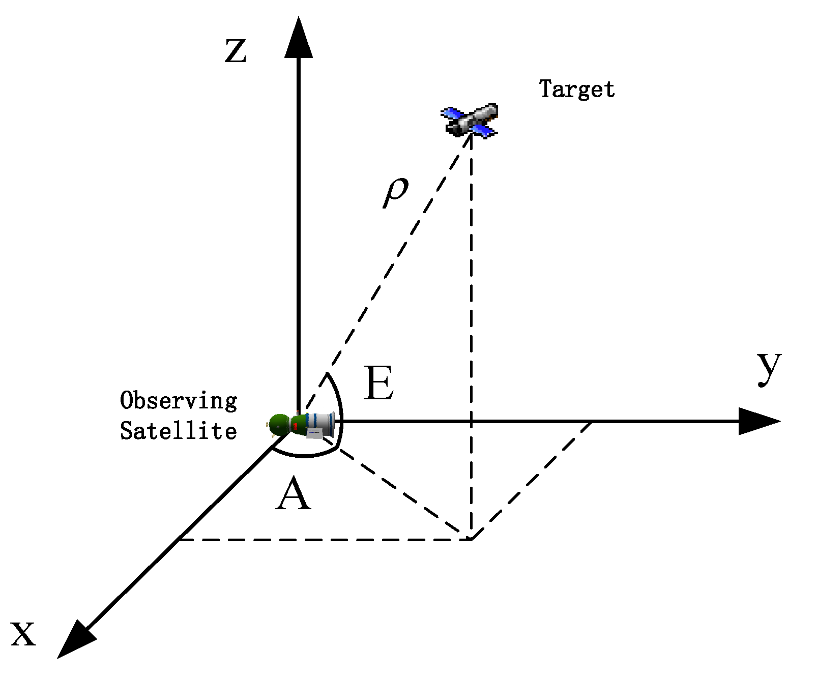
In this study, the Vehicle Velocity and Local Horizontal (VVLH) coordinate system is used to describe the relative motion between the observing satellite and the maneuvering target. The origin of the VVLH frame is attached to the observing satellite’s centroid; the y-axis points to the direction of the negative normal to the orbital plane, the z-axis points to the center of the earth, and the x-axis satisfies the right-handed rule. In the VVLH coordinate system, the elevation angle E is defined as the angle between the line-of-sight and the x–y plane; the azimuth angle A is defined as the angle between the projection of line-of-sight in the x–y plane and the x-axis direction, and it takes the x-axis as the starting point to rotate counterclockwise as positive (see in Figure 1).

Then the observation equation can be described as

$$Z=\left[\begin{array}{c}\rho \\ E\\ A\end{array}\right]=h(\mathit{X})=\left[\begin{array}{c}\sqrt{x^2+y^2+z^2}\\ {\tan }^{-1}\frac{z}{\sqrt{x^2+y^2}}\\ {\tan }^{-1}\frac{y}{x}\end{array}\right]$$

(14)

Additionally, the observation matrix can be derived as

$$H=\frac{\partial h(\mathit{X})}{\partial {\mathit{X}}^{\mathrm{T}}}=\left[\begin{array}{cccc}{H}_{11}& H_{12}& H_{13}& \\ H_{21}& H_{22}& H_{23}& {\mathbf{0}}_{9\times 3}\\ H_{31}& H_{32}& H_{33}& \end{array}\right]$$

(15)

where

$$H_{11}=\frac{x}{\sqrt{x^2+y^2+z^2}}$$

$$H_{12}=\frac{y}{\sqrt{x^2+y^2+z^2}}$$

$$H_{13}=\frac{z}{\sqrt{x^2+y^2+z^2}}$$

$$H_{21}=\frac{-xz}{\sqrt{x^2+y^2}(x^2+y^2+z^2)}$$

$$H_{22}=-\frac{yz}{\sqrt{x^2+y^2}(x^2+y^2+z^2)}$$

$$H_{23}=\frac{\sqrt{x^2+y^2}}{x^2+y^2+z^2}$$

$$H_{31}=\frac{-y}{x^2+y^2}$$

$$H_{32}=\frac{x}{x^2+y^2}$$

2.3. Maneuvering Acceleration Model

It is known from the fundamentals of orbital dynamics that the estimated value of acceleration in the relative motion represented by Equation (8) is a total acceleration value, which contains the relative gravitational acceleration and the relative maneuvering acceleration. For the spacecraft orbital pursuit–evasion game, it is of great significance for the observing satellite to identify the maneuvering acceleration of the target in real-time so as to implement security defense strategies. The process of solving the maneuvering acceleration of the target in the VVLH frame is given below.

According to the composition theorem of acceleration, the acceleration of the maneuvering target relative to the observing satellite can be expressed as

$${\mathit{a}}_c-{\mathit{a}}_o={\mathit{a}}_{rel}+\mathit{\epsilon }\times {\mathit{r}}_{rel}+\mathit{\omega }\times (\mathit{\omega }\times {\mathit{r}}_{rel})+2\mathit{\omega }\times {\mathit{v}}_{rel}$$

(16)

where ${\mathit{a}}_c$ is the absolute acceleration of the maneuvering target, ${\mathit{a}}_o$ is the absolute acceleration of the observing satellite, and ${\mathit{a}}_{rel}$ is the relative acceleration of the maneuvering target to the observing satellite. $\mathit{\omega }$ and $\epsilon$ are the angular velocity and angular acceleration of the observing satellite, respectively. ${\mathit{r}}_{rel}$ and ${\mathit{v}}_{rel}$ are the relative position and velocity vectors, respectively, between the maneuvering target and the observing satellite.

The acceleration of the maneuvering target consists of two parts, namely gravitational acceleration ${\mathit{a}}_{cg}$ and maneuvering acceleration ${\mathit{a}}_{cf}$, and

$${\mathit{a}}_c={\mathit{a}}_{cg}+{\mathit{a}}_{cf}$$

(17)

Under the two-body hypothesis, the gravitational acceleration satisfies

$${\mathit{a}}_{cg}=-\frac{\mu }{{\mathit{r}}_c^3}{\mathit{r}}_c$$

(18)

where ${\mathit{r}}_c$ is the absolute position of the target. The relative states can be replaced by the values estimated: ${\mathit{r}}_{rel}={\widehat{\mathit{r}}}_{rel}$, ${\mathit{v}}_{rel}={\widehat{\mathit{v}}}_{rel}$, ${\mathit{a}}_{rel}={\widehat{\mathit{a}}}_{rel}$, ${\mathit{r}}_c={\widehat{\mathit{r}}}_c={\mathit{r}}_o+{\widehat{\mathit{r}}}_{rel}$, and ${\mathit{r}}_o$ is the absolute position of the observing satellite. Therefore, ${\widehat{\mathit{a}}}_{cg}=-\mu {\widehat{\mathit{r}}}_c/{\widehat{\mathit{r}}}_c^3$. Substituting it into Equation (16) yields

$${\widehat{\mathit{a}}}_{cf}={\widehat{\mathit{a}}}_{rel}-{\widehat{\mathit{a}}}_{cg}+{\mathit{a}}_o+\mathit{\epsilon }\times {\widehat{\mathit{r}}}_{rel}+\mathit{\omega }\times (\mathit{\omega }\times {\widehat{\mathit{r}}}_{rel})+2\mathit{\omega }\times {\widehat{\mathit{v}}}_{rel}$$

(19)

If the observing satellite does not maneuver, it flies approximately along the Keplerian orbit within a filtering period. Then we have

$${\mathit{a}}_o={\mathit{a}}_{og}=-\frac{\mu }{{\mathit{r}}_o^3}{\mathit{r}}_o$$

(20)

$$\mathit{\omega }=\frac{{\mathit{r}}_o\times {\mathit{v}}_o}{{\mathit{r}}_o^2}=\frac{{\mathit{h}}_o}{{\mathit{r}}_o^2}$$

(21)

$$\mathit{\epsilon }=\dot{\mathit{\omega }}=\frac{-2({\mathit{r}}_o\cdot {\mathit{v}}_c) ({\mathit{r}}_o\times {\mathit{v}}_o)}{{\mathit{r}}_o^4}$$

(22)

where ${\mathit{a}}_{og}$ and ${\mathit{v}}_o$ are the gravitational acceleration the absolute velocity of the observing satellite. Substituting Equations (20)–(22) into Equation (19), then the estimated value of ${\widehat{\mathit{a}}}_{cf}$ can be obtained.

If the observing satellite maneuvers, generally the maneuvering acceleration of the spacecraft is small, so it can be considered that the angular momentum of the observing satellite is a constant vector within each simulation step. Therefore,

$${\mathit{a}}_o={\mathit{a}}_{og}+{\mathit{a}}_{of}=-\frac{\mu }{{\mathit{r}}_o^3}{\mathit{r}}_o+{\mathit{a}}_{of}$$

(23)

$$\mathit{\omega }=\frac{{\mathit{r}}_o\times {\mathit{v}}_o}{{\mathit{r}}_o^2}=\frac{{\mathit{h}}_o}{{\mathit{r}}_o^2}$$

(24)

$$\mathit{\epsilon }=\dot{\mathit{\omega }}=\frac{{\mathit{r}}_o^2({\mathit{r}}_o\times {\mathit{a}}_{of})-2({\mathit{r}}_o\cdot {\mathit{v}}_o) ({\mathit{r}}_o\times {\mathit{v}}_o)}{{\mathit{r}}_o^4}$$

(25)

where ${\mathit{a}}_{of}$ is the maneuvering acceleration of the observing satellite. Substituting Equations (23)–(25) into Equation (19), then the estimated value of ${\widehat{\mathit{a}}}_{cf}$ can be obtained.

3. Adaptive Tracking Algorithm for Continuously Thrusting Spacecraft

3.1. Introduction to CSJerk-Based EKF Filtering

The CSJerk model is a linear model, and the observation model is a non-linear model. The EKF algorithm is used to estimate the relative states of the target based on the CSJerk model. The estimated state is a 12-dimensional vector, including 3 relative position components, 3 relative velocity components, 3 relative acceleration components, and 3 jerk components. The CSJerk-based EKF algorithm has the following steps within one filtering period:

Step 1: Determining the initial estimation ${\widehat{\mathit{X}}}_0$ and ${\widehat{\mathit{P}}}_0$

$${\widehat{\mathit{X}}}_0=E[{\mathit{X}}_0]$$

(26)

$${\widehat{\mathit{P}}}_0=E\left[({\mathit{X}}_0-{\widehat{\mathit{X}}}_0){({\mathit{X}}_0-{\widehat{\mathit{X}}}_0)}^{\mathrm{T}}\right]$$

(27)

Step 2: Updating the state mean and covariance matrix

(1)

The prediction of relative state $\mathit{X}(k+1,k)$

$$\mathit{X}(k+1,k)=\mathit{\Phi }(k+1,k)\widehat{\mathit{X}}(k)+U(k)$$

(28)

where $\mathit{\Phi }(k+1,k)$ and $U(k)$ are associated with Equations (A3) and (A4) in Appendix A.

(2)

The covariance matrix $\mathit{P}(k+1,k)$

$$\mathit{P}(k+1,k)=\mathit{\Phi }(k+1,k)\widehat{\mathit{P}}(k)\mathit{\Phi }{(k+1,k)}^{\mathrm{T}}+Q(k)$$

(29)

Step 3: Updating the measurement

(1)

The gain matrix $K(k+1)$

$$K(k+1)=\mathit{P}(k+1,k)H{(k+1)}^{\mathrm{T}}[H(k+1)\mathit{P}(k+1,k))H{(k+1)}^{\mathrm{T}}+R(k+1){]}^{-1}$$

(30)

$$H(k+1)=\frac{\partial h}{\partial \mathit{X}}{|}_{\mathit{X}(k+1,k)}$$

(31)

(2)

The estimations $\widehat{\mathit{X}}(k+1)$ and $\widehat{\mathit{P}}(k+1)$.

$$\widehat{\mathit{X}}(k+1)=\mathit{X}(k+1,k)+K(k+1)v(k+1)$$

(32)

$$v(k+1)=z(k+1)-h(\mathit{X}(k+1,k))$$

(33)

$$\widehat{\mathit{P}}(k+1)=(I-K(k+1)H(k+1))\mathit{P}(k+1,k)$$

(34)

3.2. Improved CSJerk Filtering Algorithm Based on Residual-Normalized Orthogonalization

If the maneuvering parameters of the CSJerk filtering match the actual values, the EKF algorithm based on the CSJerk model can track the target stably. However, for the non-cooperative spacecraft, its maneuvering information is unknown. Moreover, due to the abrupt change of the target maneuvering acceleration, the values set according to the prior information may not match the maneuvering change of the target, which will make the filter suffer from degradation and even divergence. In order to address this problem, this paper combines the idea of residual-normalized orthogonalization with CSJerk-based EFK filtering, and a robust CSJerk filtering algorithm is developed.

The principle of traditional strong tracking is to make the residual $v$ orthogonal to each other in each step [30].

$$E\left[{({\mathit{v}}_{k+1+j})}^{\mathrm{T}}({\mathit{v}}_{k+1})\right]=0\hspace{1em}\hspace{1em}\hspace{1em}\hspace{1em}j=1,2, \dots ,n$$

(35)

However, the residual orthogonalization principle has different sensitivity to different residual components because the change magnitude of the range and angle measurement are different when the target executes maneuvers, which makes the filter not able to detect the state change quickly and accurately. To deal with this shortcoming, Jiang et al. [31] proposed a method to normalize the residual vector before orthogonalization.

$$E\left[{(\mathit{M}{v}_{k+1+j})}^{\mathrm{T}}(\mathit{M}{v}_{k+1})\right]=0\hspace{1em}\hspace{1em}\hspace{1em}\hspace{1em}j=1,2,\dots ,n$$

(36)

where $\mathit{M}=\mathrm{diag}({\sigma }_{\rho }^{-1} {\sigma }_A^{-1} {\sigma }_E^{-1})$ is the weighting matrix.

Inspired by Jiang et al. [31], this note combines the idea of residual-normalized orthogonalization with EFK based on the CSJerk model. According to Section 3.1, the improved filtering algorithm is as follows:

$${\mathit{P}}^{\ast }(k+1,k)={\lambda }_{k+1}\mathit{\Phi }(k+1,k)\widehat{\mathit{P}}(k)\mathit{\Phi }{(k+1,k)}^{\mathrm{T}}+Q(k)$$

(37)

$$K^{\ast }(k+1)={\mathit{P}}^{\ast }(k+1,k)H{(k+1)}^{\mathrm{T}}[H(k+1){\mathit{P}}^{\ast }(k+1,k))H{(k+1)}^{\mathrm{T}}+R(k+1){]}^{-1}$$

(38)

$$\widehat{\mathit{X}}(k+1)=\mathit{X}(k+1,k)+K^{\ast }(k+1)v(k+1)$$

(39)

$$\widehat{\mathit{P}}(k+1)=(I-K^{\ast }(k+1)H(k+1)){\mathit{P}}^{\ast }(k+1,k)$$

(40)

where ${\lambda }_{k+1}$ is a fading factor to amplify the covariance when a maneuver occurs, and it can be derived by the principle of residual-normalized orthogonalization [31].

$${\lambda }_{k+1}=\{\begin{array}{cc}1,\hfill & {\alpha }_{k+1}\le 1\hfill \\ {\alpha }_{k+1},\hfill & {\alpha }_{k+1}>1\hfill \end{array}$$

(41)

$${\alpha }_{k+1}=\frac{tr[(V_{k+1}-R){\mathit{M}}^2]}{tr[(H_{k+1}{\mathit{\Phi }}_{k+1,k}{\widehat{\mathit{P}}}_k{\mathit{\Phi }}_{k+1,k}^{\mathrm{T}}{H}_{k+1}^{\mathrm{T}}){\mathit{M}}^2]}$$

(42)

$$V_{k+1}=E({\mathit{v}}_{k+1}{\mathit{v}}_{k+1}^T)\approx \{\begin{array}{cc}{\mathit{v}}_1{\mathit{v}}_1^{\mathrm{T}},\hfill & \mathrm{k}=0\hfill \\ \frac{\rho V_k+{\mathit{v}}_{k+1}{\mathit{v}}_{k+1}^{\mathrm{T}}}{1+\rho },\hfill & \mathrm{k}\ge 1\hfill \end{array}$$

(43)

where $0<\rho \le 1$ is a forgetting factor, and it is re-commanded as $\rho =0.95$ in default. So far, the RCSJF method can be described by Equations (26)–(28) and (37)–(43).

3.3. IMM Algorithm Based on RCSJF

In Section 3.2, by combining the idea of residual-normalized orthogonalization with CSJerk-based EKF, the RCSJF is proposed, which enhances the robustness of tracking a target with abrupt state changes. In order to extend its applicability for different maneuver levels, this paper uses the RCSJF algorithms with different maneuver frequencies and maximum jerk values to form the model set of the IMM. With this model set, an adaptive IMM filtering algorithm based on RCSJF is developed.

The standard IMM algorithm contains four modules [32]: input mixing, model-conditioned estimation, model probability update, and comprehensive output. The recursive steps from time $k$ to $k+1$ are given as follows:

Step 1: Input Mixing

Assuming the estimation of filter $i$ $(i=1,2,3)$ is ${\widehat{\mathit{X}}}^i(k)$ at time $k$ $(k=1,2,3\dots n)$ with the covariance ${\widehat{\mathit{P}}}^i(k)$, then the input of filter $j$ $(j=1,2,3)$ after interactive calculation can be expressed as

$${\mathit{X}}^{0j}(k)={\displaystyle \sum _{i=1}^3{m}^{i|j}(k)}{\widehat{\mathit{X}}}^i(k)$$

(44)

$${\mathit{P}}^{0j}(k)={\displaystyle \sum _{i=1}^3{m}^{i|j}(k)}\times \{{\widehat{\mathit{P}}}^i(k)+[{\widehat{\mathit{X}}}^i(k)-{\mathit{X}}^{0j}(k)]{[{\widehat{\mathit{X}}}^i(k)-{\mathit{X}}^{0j}(k)]}^{\mathrm{T}}\}$$

(45)

where $m^{i|j}(k)$ is the mixing probability from the filter $i$ to $j$, and it can be computed as

$$m^{i|j}(k)=\frac{{\gamma }_{ij}{m}^i(k)}{{\displaystyle {\sum }_{i=1}^3{\gamma }_{ij}{m}^i(k)}}$$

(46)

where $m^i$ is the model probability, and the model transition probability ${\gamma }_{ij}$ is a constant value designed according to a priori information.

Step 2: Model-Conditioned Estimation

Substitute the mixed values calculated in step 1 into the sub-filters of the model set to obtain the estimation of ${\widehat{\mathit{X}}}^j(k+1)$ and covariance ${\mathit{P}}^j(k+1)$ of each model

$${\mathit{X}}^j(k+1,k)={\mathit{\Phi }}^j(k+1,k){\mathit{X}}^{0j}(k)+U^j(k)\overline{j}$$

(47)

$${\mathit{P}}^j(k+1,k)={\lambda }_{k+1}^j{\mathit{\Phi }}^j(k+1,k){\mathit{P}}^{0j}(k){\mathit{\Phi }}^j{(k+1,k)}^{\mathrm{T}}+Q^j(k)$$

(48)

$${\widehat{\mathit{X}}}^j(k+1)={\mathit{X}}^j(k+1,k)+K(k+1){\mathit{v}}^j(k+1)$$

(49)

$${\mathit{v}}^j(k+1)=\mathit{y}(k+1)-h({\mathit{X}}^j(k+1,k))$$

(50)

$${\widehat{\mathit{P}}}^j(k+1)=(I-K^j(k+1)H^j(k+1)){\mathit{P}}^j(k+1,k)$$

(51)

$$K^j(k+1)={\mathit{P}}^j(k+1,k))H^j{(k+1)}^{\mathrm{T}}[H^j(k+1){\mathit{P}}^j(k+1,k))H^j{(k+1)}^{\mathrm{T}}+R(k+1){]}^{-1}$$

(52)

$$H^j(k)=\frac{\partial \mathit{h}}{\partial \mathit{X}}{|}_{{\mathit{X}}^j(k+1,k)}$$

(53)

Step 3: Model Probability Update

Assuming that the residual ${\mathit{v}}^j(k+1)$ is according to a Gaussian distribution with covariance ${\mathit{S}}^j(k+1)$, then the model likelihood function ${\mathit{\Lambda }}^j(k+1)$ and model probability $m^j(k+1)$ can be updated as

$${\mathit{\Lambda }}^j(k+1)=\frac{1}{\sqrt{\left|2\pi S^j(k+1)\right|}}\exp {\{-\frac{1}{2}{[v^j(k+1)]}^{\mathrm{T}}(S^j(k+1)])}^{-1}[v^j(k+1)]\}$$

(54)

$$m^j(k+1)=\frac{1}{C}{\mathit{\Lambda }}^j(k+1){\overline{C}}_j$$

(55)

where $C={\displaystyle \sum _{j=1}^3{\mathit{\Lambda }}^j(k+1)}{\overline{C}}_j$, ${\overline{C}}_j={\displaystyle {\sum }_{j=1}^3{\gamma }_{ij}(k)m^j(k)}$, ${\mathit{v}}^j(k+1)$ and ${\mathit{S}}^j(k+1)$ are calculated as

$${\mathit{v}}^j(k+1)=Z(k+1)-\mathit{h}({\mathit{X}}^j(k+1,k))$$

(56)

$$S^j(k+1)=H^j(k+1){\mathit{P}}^j(k+1,k))H^j{(k+1)}^{\mathrm{T}}+R(k+1)$$

(57)

Step 4: Comprehensive Output

The estimated state $\widehat{\mathit{X}}(k+1)$ and its covariance $\widehat{\mathit{P}}(k+1)$ can be expressed by the model probability and the update of each model

$$\widehat{\mathit{X}}(k+1)={\displaystyle \sum _{j=1}^3{\widehat{\mathit{X}}}^j(k+1)m^j(k+1)}$$

(58)

$$\widehat{\mathit{P}}(k)={\displaystyle \sum _{j=1}^3\{{\widehat{\mathit{P}}}^j(k+1)+[{\widehat{\mathit{X}}}^j(k+1)-\widehat{\mathit{X}}(k+1)]}{[{\widehat{\mathit{X}}}^j(k+1)-\widehat{\mathit{X}}(k+1)]}^{\mathrm{T}}\}{m}^j(k+1)$$

(59)

4. Results

To validate the proposed method, simulations were designed from two aspects. First, the feasibility of the RCSJF was verified. Assuming that the maneuvering target executes a constant thrust maneuver during the approaching process, the changes of the algorithm tracking error between the CSJerk-based EKF and RCSJF were compared. Second, the applicability of the IMM algorithm based on RCSJF was verified by different maneuvering conditions. Three constant maneuvering conditions and three time-varying maneuvering conditions were set for the maneuvering target in the simulation. The magnitude of the maneuvering amplitude was different for the constant maneuvering condition while the maneuvering amplitude, frequency, and phase were different for the time-varying maneuvering condition.

4.1. Simulation Setups

Assume that the maneuvering target approaches the observing satellite by maneuvering with continuous thrusts. Both of them run on the orbits with the parameters shown in

Table 1. Initial orbital elements of the observing satellite and maneuvering target.

Parameters	a (km)	e	i (°)	Ω (°)	w (°)	f (°)
Observing satellite	42,175.14	0.002	1.37	359.12	−113.12	184.52
Maneuvering target	42,165.14	0.008	1.38	359.12	−113.12	184.80

, and the initial error is defined with mean ${\mathit{X}}_{error}={[{10}^3 {10}^3 {10}^3 {10}^1 {10}^1 {10}^1 {10}^{-4} {10}^{-4} {10}^{-4} {10}^{-4} {10}^{-4}]}^{\mathrm{T}}$ and covariance $\mathit{P}=diag([{10}^3 {10}^3 {10}^3 {10}^1 {10}^1 {10}^1 {10}^{-2} {10}^{-2} {10}^{-2} {10}^{-2} {10}^{-2} {10}^{-2}])$. In Table 1, the parameters a, e, i, Ω, w, and f denote the orbit elements of the semimajor axis, eccentricity, inclination, longitude of the ascending node, argument of perigee, and true anomaly, respectively. The observing satellite uses an optical camera and a laser ranger to measure the maneuvering target, the elevation angle, and azimuth angle, and the relative distance can be obtained in real time. The observing satellite uses this information to estimate the relative state and the maneuvering acceleration of the target. In the simulations, the measurement errors and the measurement frequency of the observing satellite are set as ${\sigma }_{\rho }=10 \mathrm{m}$, ${\sigma }_A={\sigma }_E=0.001 \mathrm{rad}$, and $f=1 \mathrm{Hz}$, respectively. Additionally, the smaller the measurement error or the higher the observation frequency, the higher the accuracy, but they are limited by the sensors.

4.2. Analysis of the Residual-Normalized Orthogonalization

To analyze the effectiveness of the RCSJF algorithm, assume that the target maneuvers during the time from $t=1000 \mathrm{s}$ to $t=2000 \mathrm{s}$, and the acceleration vector in VVLH is set as ${\left[-0.2 \mathrm{m}/{\mathrm{s}}^2,0 \mathrm{m}/{\mathrm{s}}^2,0.2 \mathrm{m}/{\mathrm{s}}^2\right]}^{\mathrm{T}}$. The maneuvering frequency and the maximum jerk value of CSJerk are specified as $\alpha =0.001$ and $j_{\max }={10}^{-4}$, respectively. Generally, $\alpha$ and $j_{\max }$ permit one to model targets with different levels of thrust: small $\alpha$ and $j_{\max }$ for targets with enduring jerk, and high $\alpha$ and $j_{\max }$ for target with rapidly fluctuating jerk [29].

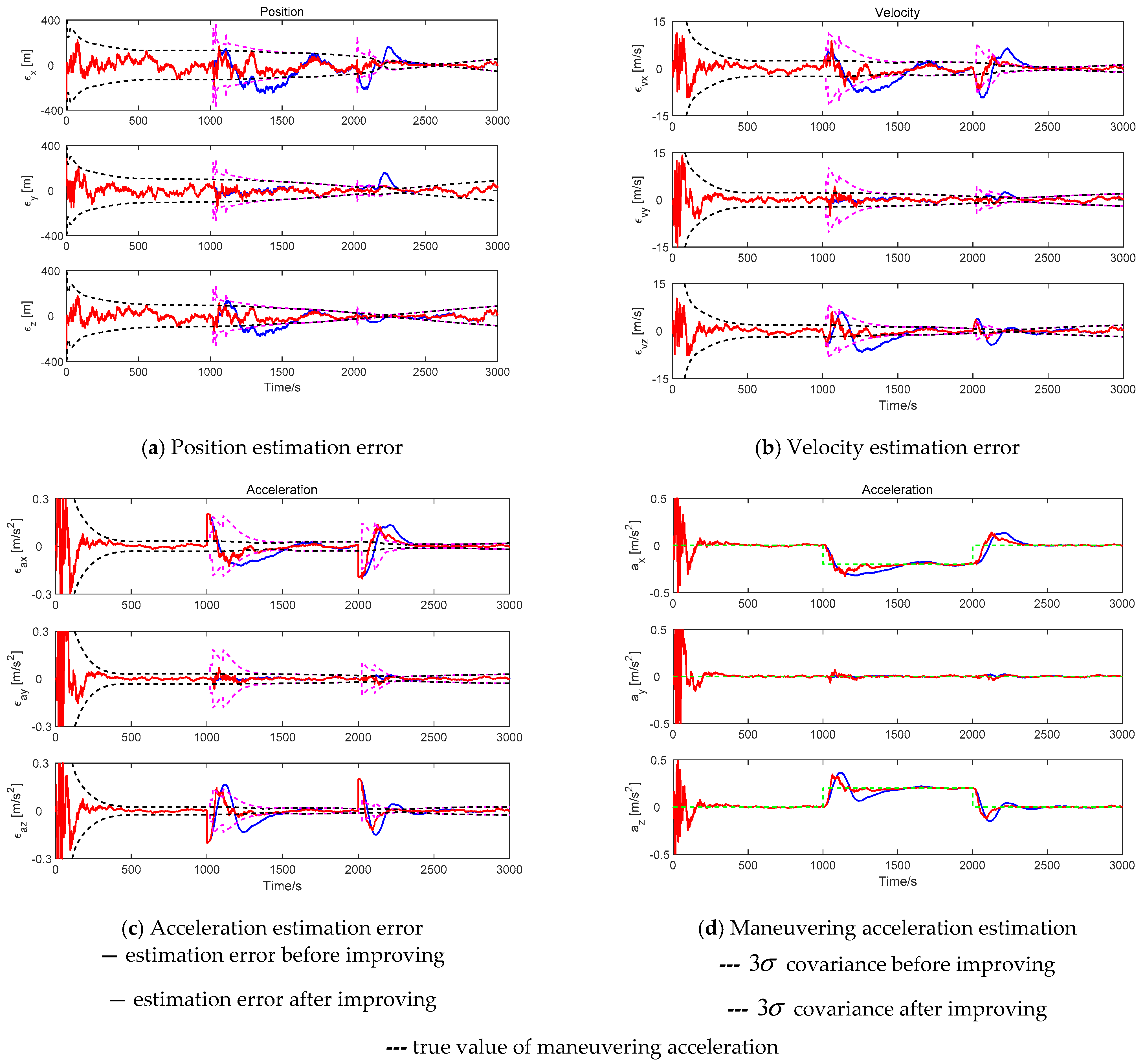
The sub-graphs (a)–(c) in Figure 2 show the error changes in the estimation results of maneuvering target before and after improving the CSJerk-based EKF filtering algorithm by residual-normalized orthogonalization. The sub-graph (d) shows the maneuvering acceleration estimation of the maneuvering target. As shown in Figure 2, before the improvement of residual-normalized orthogonalization, the estimation errors of all position, velocity, and acceleration are beyond the scale described by $\pm 3\sigma$ values when the maneuver starts or ends and stabilize $500 \mathrm{s}$ later. However, after the improvement, the estimation errors are reduced and basically remain within the scale described by $\pm 3\sigma$ values and stabilize about $200 \mathrm{s}$ later. It is evident that the ability to converge is significantly improved. The effect of the residual-normalized orthogonalization is that when the state changes abruptly, the residual sequences are sensitive to this change, which makes the fading factor change adaptively, thereby inflating the prediction covariance to maintain filter stability and then improve the convergence effect.

4.3. Analysis of the IMM Algorithm Based on RCSJF

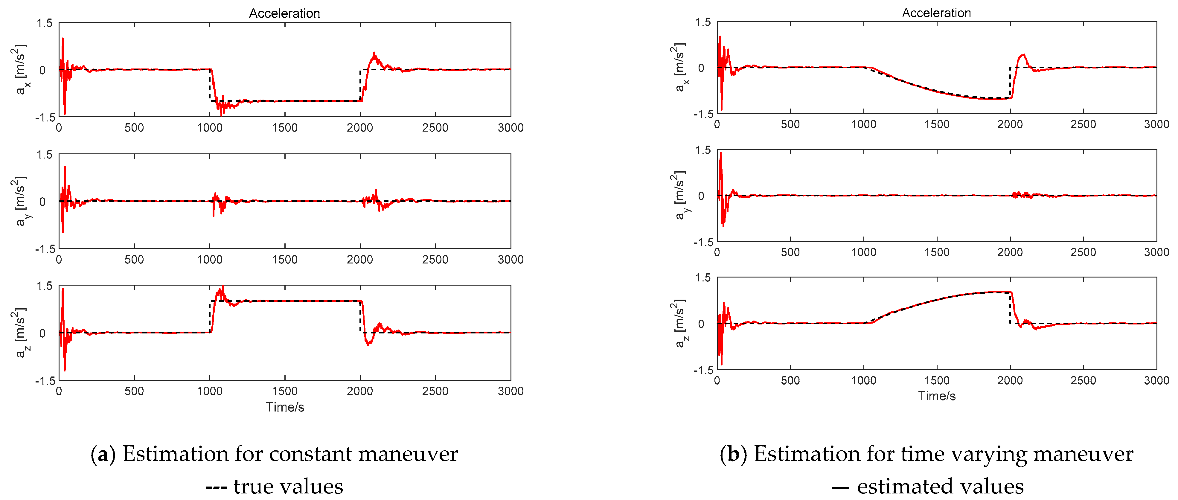
To demonstrate the applicability of the IMM algorithm based on RCSJF in this paper, a variety of maneuver conditions was considered. The constant maneuvering scenarios are set in

Table 2. Maneuver levels for constant maneuver.

Conditions	$\mathbf{Size} ({\mathbf{m}/\mathbf{s}}^2)$	Time (s)	$\mathit{x}({\mathbf{m}/\mathbf{s}}^2)$	$\mathit{y}({\mathbf{m}/\mathbf{s}}^2)$	$\mathit{z}({\mathbf{m}/\mathbf{s}}^2)$
1	0.141	1000–2000	−0.1	0	0.1
2	0.707	1000–2000	−0.5	0	0.5
3	1.414	1000–2000	−1	0	1

, while the time-varying maneuvering scenarios are set in

Table 3. Maneuver levels for time-varying maneuver.

Conditions	Time (s)	$\mathit{x}({\mathbf{m}/\mathbf{s}}^2)$	$\mathit{y}({\mathbf{m}/\mathbf{s}}^2)$	$\mathit{z}({\mathbf{m}/\mathbf{s}}^2)$
1	1000–2000	$-0.1\sin (0.3t-200)$	0	$0.1\sin (0.3t-200)$
2	1000–2000	$-0.5\sin (0.2t-100)$	0	$0.5\sin (0.2t-100)$
3	1000–2000	$-\sin (0.1t-100)$	0	$\sin (0.1t-100)$

. For the constantly maneuvering case, the influence of maneuver size was compared; for the time-varying maneuvering case, all three, namely maneuvering amplitude, frequency, and initial phase, were analyzed in the conditions.

For the IMM algorithm based on RCSJF, the maneuvering frequency is $\tilde{\alpha }=0.001$, and the maximum jerk values of the three models in the IMM algorithm are set as $j_{\max 1}={10}^{-6},j_{\max 2}={10}^{-4},j_{\max 3}={10}^{-3}$, which are responsible for different levels of thrust, respectively. The IMM model transition probability matrix ${\mathit{M}}_{\gamma }$ determines the proportion of each model output in the step of input mixing. Usually, the target is in the state with no maneuvers, so ${\mathit{M}}_{\gamma }$ is set to

$${\mathit{M}}_{\gamma }=\left[\begin{array}{ccc}0.5& 0.25& 0.25\\ 0.25& 0.5& 0.25\\ 0.25& 0.25& 0.5\end{array}\right]$$

(60)

At the beginning of the simulation, the importance of each model is considered to be consistent, thus the model probability is set as $m_j(0)=0.333$. The filter estimation initial value ${\widehat{\mathit{X}}}^j$ and initial covariance matrix ${\mathit{P}}^j$ of each model are set as

$${\widehat{\mathit{X}}}^j(0)=\mathit{X}(0)+{\mathit{X}}_{error}$$

(61)

$${\mathit{P}}^j(0)=diag([{10}^6 {10}^6 {10}^6 {10}^2 {10}^2 {10}^2 {10}^{-2} {10}^{-2} {10}^{-2} {10}^{-2} {10}^{-2} {10}^{-2}])$$

(62)

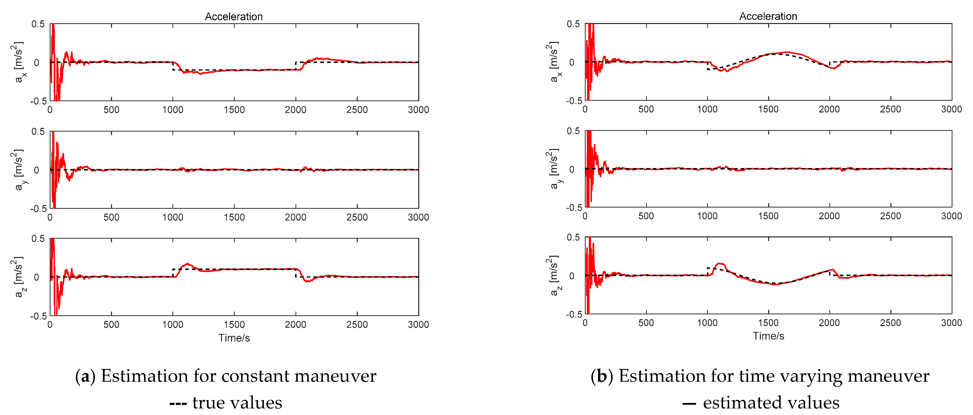
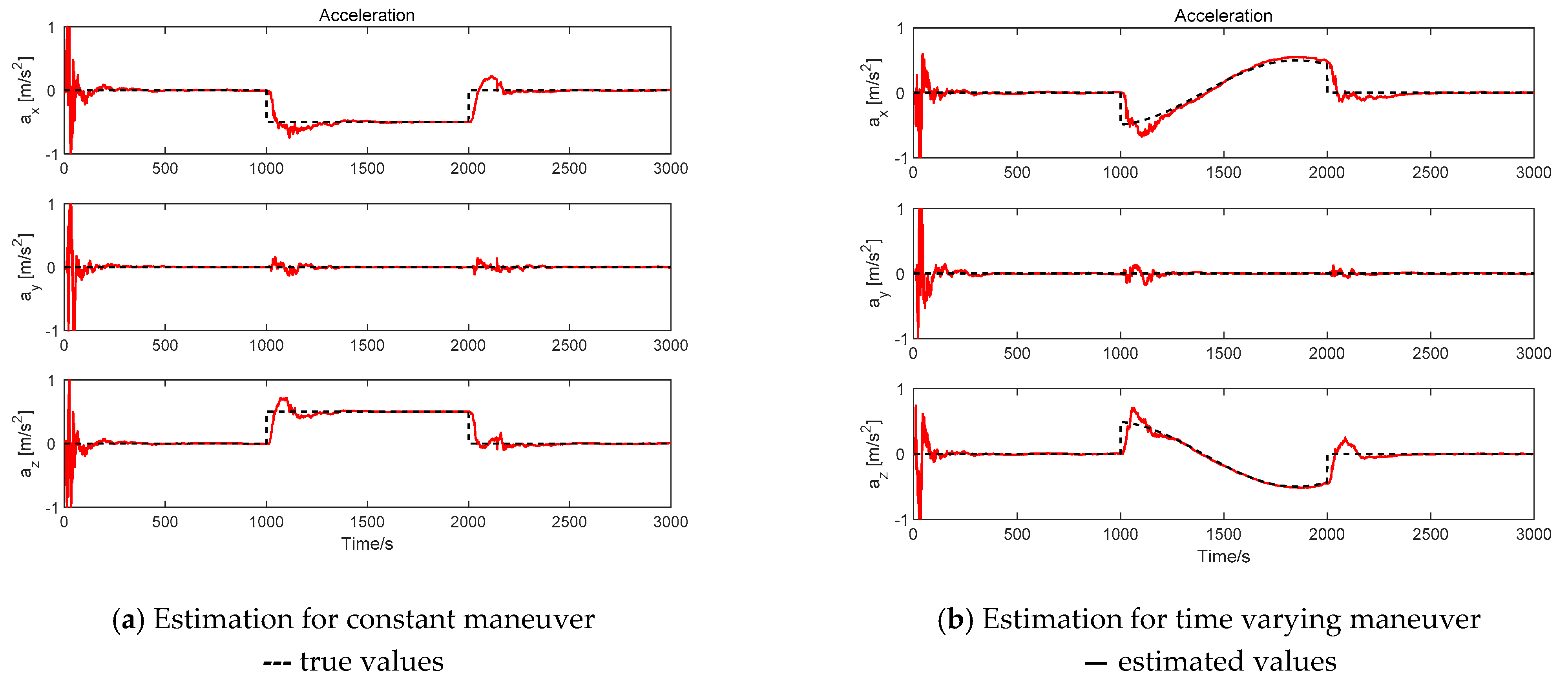
This section focuses on the estimated maneuvering acceleration of the target under different maneuver conditions. As shown in Figure 3, Figure 4 and Figure 5, the proposed algorithm can effectively estimate the component values of the maneuvering acceleration for both constant maneuvering and time-varying maneuvering conditions, and it converges about $200 \mathrm{s}$ later when the enginehen the maneuvering acceleration amplitude of the target is larger, the abrupt change of state is more obvious, the residual sequences react more quickly, and the errors are adjusted more quickly, but the process changes more drastically. As shown in sub-graph (a) of Figure 3, Figure 4 and Figure 5, when the amplitude of the maneuver increases, the acceleration estimation curve changes more drastically and converges to the true value curve faster after the maneuver starts or ends (at $1000 \mathrm{s}$ and $2000 \mathrm{s}$). For time-varying maneuvering, the influence produced by the change of maneuver amplitude is consistent with the constant maneuvering. However, the acceleration curve estimated can track the true curve stably when the acceleration phase executed by the target is 0; that is, the maneuvering acceleration changes continuously from zero with no mutation, just as shown in Figure 5b for Condition 3.

5. Conclusions

In this paper, an adaptive IMM algorithm based on RCSJF is proposed to track non-cooperative spacecraft with continuous thrusts. The CSJerk-based EKF filter typically has poor estimation accuracy when an unknown maneuver occurs or ends with no prior information. To address this problem, this study applies the idea of residual-normalized orthogonalization to the EKF based on the CSJerk model, by which the RCSJF algorithm is obtained. On the other hand, there is no idea for the maneuvers performed by the target, so it is difficult to determine the parameters of the CSJerk model. Therefore, an IMM algorithm that takes the RCSJF with different levels of maneuvering parameters as the model set is designed to adapt to the uncertain maneuvers of the target. Simulation results show that the CSJerk-based EKF filtering algorithm improved by the residual-normalized orthogonalization (i.e., RCSJF) can enhance the robustness of the single-model algorithm, and the proposed IMM algorithm based on RCSJF can effectively estimate the maneuvering acceleration of the target that executes different levels of maneuvers, even for time-varying maneuvers with different amplitudes and frequencies. Moreover, the proposed adaptive tracking method has potential benefit to accurately distinguish the control regulation of a maneuvering target, which is of great significance for improving the survivability of the on-orbit spacecraft.

Several limitations of the proposed method are observed. First, since the jerk information of the non-cooperative target is unknown, the maneuvering parameters ($j_{\max }$ and $\alpha$) for the CSJerk-based EKF filtering algorithm may not be in accordance with the actual situation. Second, although the IMM method with three CSJerk-based EKF filters deals with the problem of parameter uncertainty to some extent, more model components will be required, and the computational complexity will increase as the uncertainty in maneuver magnitude (or other parameters) becomes larger. Consequently, the ability to deal with parameters with very large uncertainties may be computationally extensive. Therefore, our next research direction will focus on solving these problems.

References

- Ho, C.C.; McClamroch, N.H. Automatic spacecraft docking using computer vision-based guidance and control techniques. J. Guid. Control Dyn. 1993, 16, 281–288. [Google Scholar] [CrossRef] [Green Version]
- Philip, N.K.; Ananthasayanam, M.R. Relative position and attitude estimation and control schemes for the final phase of an autonomous docking mission of spacecraft. Acta Astronaut. 2003, 52, 511–522. [Google Scholar] [CrossRef]
- Zhou, J.P. Space Rendezvouse and Docking Technology, 1st ed.; National Defense Industry Press: Beijing, China, 2013; pp. 179–185. (In Chinese) [Google Scholar]
- Shoemaker, J.; Wright, M. Orbital express space operations architecture program. In Proceedings of the Spacecraft Platforms and Infrastructure, Orlando, FL, USA, 30 August 2004; Volume 5419, pp. 57–65. [Google Scholar]
- Available online: https://directory.eoportal.org/web/eoportal/satellite-missions/m/mev-1 (accessed on 12 June 2021).
- Carr, R.W.; Cobb, R.G.; Pachter, M.; Pierce, S. Solution of a Pursuit–Evasion Game Using a Near-Optimal Strategy. J. Guid. Control Dyn. 2018, 41, 1–10. [Google Scholar] [CrossRef]
- Li, Z.; Zhu, H.; Yang, Z. Saddle Point of Orbital Pursuit-Evasion Game Under J 2-Perturbed Dynamics. J. Guid. Control Dyn. 2020, 43, 1733–1739. [Google Scholar] [CrossRef]
- Holzinger, M.; Scheeres, D. Applied reachability for space situational awareness and safety in spacecraft proximity operations. In Proceedings of the AIAA Guidance, Navigation, and Control Conference, Chicago, IL, USA, 10–13 August 2009. [Google Scholar]
- Wen, C.; Peng, C.; Gao, Y. Reachable domain for spacecraft with ellipsoidal Delta-V distribution. Astrodynamics 2018, 2, 265–288. [Google Scholar] [CrossRef]
- Bobrinsky, N.; Del Monte, L. The space situational awareness program of the European Space Agency. Cosm. Res. 2010, 48, 392–398. [Google Scholar] [CrossRef]
- Gates, R.M.; Clapper, J.R. National Security Space Strategy Unclassified Summary; US Department of Defense and Office of the Director of National Intelligence: Washington, DC, USA, 2011.
- Kennewell, J.A.; Vo, B.N. An overview of space situational awareness. In Proceedings of the 16th International Conference on Information Fusion, Istanbul, Turkey, 9–12 July 2013; pp. 1029–1036. [Google Scholar]
- Verspieren, Q. The United States Department of Defense space situational awareness sharing program: Origins, development and drive towards transparency. J. Space Saf. Eng. 2021, 8, 86–92. [Google Scholar] [CrossRef]
- Gaias, G.; D’Amico, S.; Ardaens, J.S. Angles-only navigation to a noncooperative satellite using relative orbital elements. J. Guid. Control Dyn. 2014, 37, 439–451. [Google Scholar] [CrossRef] [Green Version]
- Gong, B.; Li, W.; Li, S.; Ma, W.; Zheng, L. Angles-only initial relative orbit determination algorithm for non-cooperative spacecraft proximity operations. Astrodynamics 2018, 2, 217–231. [Google Scholar] [CrossRef]
- Ardaens, J.S.; Gaias, G. Flight demonstration of spaceborne real-time angles-only navigation to a noncooperative target in low earth orbit. Acta Astronaut. 2018, 153, 367–382. [Google Scholar] [CrossRef] [Green Version]
- Zhang, Y.; Huang, P.; Song, K.; Meng, Z. An angles-only navigation and control scheme for noncooperative rendezvous operations. IEEE Trans. Ind. Electron. 2019, 66, 8618–8627. [Google Scholar] [CrossRef]
- Goff, G.M.; Black, J.T.; Beck, J.A. Tracking maneuvering spacecraft with filter-through approaches using interacting multiple models. Acta Astronaut. 2015, 114, 152–163. [Google Scholar] [CrossRef]
- Lee, S.; Lee, J.; Hwang, I. Interacting multiple model estimation for spacecraft maneuer detection and characterization. In Proceedings of the AIAA Guidance, Navigation, and Control Conference, Kissimmee, FL, USA, 5–9 January 2015. [Google Scholar]
- Jiang, Y.Z.; Baoyin, H. Robust extended Kalman filter with input estimation for maneuver tracking. CJA. 2018, 31, 1910–1919. [Google Scholar] [CrossRef]
- Goff, G.M.; Black, J.T.; Beck, J.A. Orbit estimation of a continuously thrusting spacecraft using variable dimension filters. J. Guid. Control Dyn. 2015, 38, 2407–2420. [Google Scholar] [CrossRef]
- Kelecy, T.; Jah, M. Detection and orbit determination of a satellite executing low thrust maneuvers. Acta Astronaut. 2010, 66, 798–809. [Google Scholar] [CrossRef]
- Jiang, Y.; Baoyin, H.; Ma, P. Augmented unbiased minimum-variance input and state estimation for tracking a maneuvering satellite. Acta Astronaut. 2019, 163, 96–107. [Google Scholar] [CrossRef]
- Zhai, G.; Bi, X.Z.; Zhao, H.Y.; Liang, B. Non-cooperative maneuvering spacecraft tracking via a variable structure estimator. Aerosp. Sci. Technol. 2018, 79, 352–363. [Google Scholar]
- Singer, R.A. Estimating optimal tracking filter performance for manned maneuvering targets. IEEE Trans. Aerosp. Electron. Syst. 1970, AES-6, 473–483. [Google Scholar] [CrossRef]
- Zhou, H.R.; Kumar, K.S. A ’current’ statistical model and adaptive algorithm for estimating maneuvering targets. J. Guid. Control Dyn. 1984, 7, 596–602. [Google Scholar] [CrossRef]
- Mehrotra, K.; Mahapatra, P.R. A jerk model for tracking highly maneuvering targets. IEEE Trans. Aerosp. Electron. Syst. 1997, 33, 1094–1105. [Google Scholar] [CrossRef] [Green Version]
- Mahapatra, P.R.; Mehrotra, K. Mixed coordinate tracking of generalized maneuvering targets using acceleration and jerk models. IEEE Trans. Aerosp. Electron. Syst. 2000, 36, 992–1000. [Google Scholar] [CrossRef]
- Qiao, X.D.; Wang, B.S. A motion model for tracking highly maneuvering targets. In Proceedings of the 2002 IEEE Radar Conference, Long Beach, CA, USA, 25 April 2002; pp. 493–499. [Google Scholar]
- Zhou, D.H.; Xi, Y.G.; Zhang, Z.J. Suboptimal fading extended Kalman Filtering for nonlinear systems. Control Decis. 1990, 5, 1–6. (In Chinese) [Google Scholar]
- Jiang, Y.Z.; Ma, P.; Baoyin, H. Residual-Normalized Strong Tracking Filter for Tracking a Noncooperative Maneuvering Spacecraft. J. Guid. Control Dyn. 2019, 42, 2304–2309. [Google Scholar] [CrossRef]
- Blom, H.A.; Bar-Shalom, Y. The interacting multiple model algorithm for systems with Markovian switching coefficients. IEEE Trans. Automat. Contr. 1988, 33, 780–783. [Google Scholar] [CrossRef]
- Xiong, K.; Wei, C.L.; Liu, L.D. Robust multiple model adaptive estimation for spacecraft autonomous navigation. Aerosp. Sci Technol. 2015, 42, 249–258. [Google Scholar] [CrossRef]
- Lee, S.; Lee, J.; Hwang, I. Maneuvering Spacecraft Tracking via State-Dependent Adaptive Estimation. J. Guid. Control Dyn. 2016, 39, 2034–2043. [Google Scholar] [CrossRef]
Figure 1.
The observation coordinate system.
Figure 2.
Comparison of the estimation errors before and after the improvement of residual-normalized orthogonalization.
Figure 3.
Simulation results for Condition 1.
Figure 4.
Simulation results for Condition 2.
Figure 5.
Simulation results for Condition 3.