Article

Modeling System Risk in the South African Insurance Sector: A Dynamic Mixture Copula Approach

by
John Weirstrass Muteba Mwamba
* and
Ehounou Serge Eloge Florentin Angaman
School of Economics, University of Johannesburg, Johannesburg 2092, South Africa
*
Author to whom correspondence should be addressed.
Int. J. Financial Stud. 2021, 9(2), 29; https://0-doi-org.brum.beds.ac.uk/10.3390/ijfs9020029
Submission received: 28 January 2021 / Revised: 15 April 2021 / Accepted: 19 April 2021 / Published: 31 May 2021
(This article belongs to the Special Issue Alternative Models and Methods in Financial Economics)

Abstract

:
In this paper, a dynamic mixture copula model is used to estimate the marginal expected shortfall in the South African insurance sector. We also employ the generalized autoregressive score model (GAS) to capture the dynamic asymmetric dependence between the insurers’ returns and the stock market returns. Furthermore, the paper implements a ranking framework that expresses to what extent individual insurers are systemically important in the South African economy. We use the daily stock return of five South African insurers listed on the Johannesburg Stock Exchange from November 2007 to June 2020. We find that Sanlam and Discovery contribute the most to systemic risk, and Santam turns out to be the least systemically risky insurance company in the South African insurance sector. Our findings defy common belief whereby only banks are systemically risky financial institutions in South Africa and should undergo stricter regulatory measures. However, our results indicate that stricter regulations such as higher capital and loss absorbency requirements should be required for systemically risky insurers in South Africa.

1. Introduction

The insurance sector (life and non-life) plays a significant role in the economy and is viewed as crucial in the financial system. The European Central Bank (ECB 2013) states that insurance companies are essential for the stability of the financial system due to their investment ability, their growing links to banks, and their ability to safeguard the financial stability of households and firms by insuring their risks. In line with ECB, the National Treasury of South Africa (2011) argues that the insurance sector is a pillar of the South African financial system by being the guardian of the stability of the whole system. In addition, according to the Insurance Institute of South Africa (IISA 2016), the insurance sector (short-term and long-term insurance) accounted for 23% of total financial assets in South Africa in 2016 and contributed to R 18 billion to the country’s revenue based in 2015, implying that the insurance sector is a driver of the South African economy. Thus, a failure of one or more insurers could disrupt the insurance sector and lead to systemic risk.
Nevertheless, the International Monetary Fund (IMF 2009) has defined systemic risk as “the risk of extensive disturbance to the delivery of financial services caused by an impairment of all or parts of the financial system, which can bring about severe adverse effects on the economy”.
The 2007–2009 Global Financial Crisis (GFC) is a typical example of systemic risk. The crisis began in the United States (U.S.) real estate sector and spread to the financial system with a negative impact on economic activities across the world.
The GFC has revealed that the insurance sector was partly responsible for the crisis with American International Group (AIG) becoming the first example of an insurer in the U.S. that received federal assistance to prevent bankruptcy due to it being considered systemically risky. Thus, concerns have been raised about whether the insurance sector is a significant contributor to systemic risk. The answer to this question is capital for regulators, policymakers, investors, and academics. Hence, many studies have focused on the extent to which the insurance sector contributes to systemic risk.
For example, Grace (2011) uses granger-causality to assess the systemic risk of 12 major insurance companies in the U.S. from 2000 to 2010. The main results indicate that the insurance sector does not contribute to systemic risk because the period between its assets and liabilities is closely equaled.
Drakos and Kouretas (2015) apply the conditional value at risk (CoVaR), and the marginal conditional value at risk (ΔCoVaR) to measure systemic risk in the banking sector, insurance sector, and other financial services sectors for the U.S., and the United Kingdom (UK) between 2000 and 2012. They find that the banking sector contributes relatively more to systemic risk than the insurance sector or the other financial services in the U.S. and UK. Furthermore, based on the ΔCoVaR measures, Drakos and Kouretas (2015) argue that there is a significant increase in the contribution to systemic risk for all sectors in both countries since 2008.
Acharya and Richardson (2014) use the Credit Default Swaps Marginal Expected Shortfall (CDS-MES) as a measure of systemic risk to provide a ranking for 20 insurance companies in the U.S. with respect to their contribution to systemic risk. Their results reveal that Genworth Financial Inc., AMBAC Financial Group Inc., MBIA Inc., and AIG are the most systemically risky insurers, respectively, during the sample period, while AETNA Inc., CIGNA Corp, and Marsh & McLennan Cos. Inc. are the least systemically risky insurance companies, with CDS MESs being negative. The authors further contend that the insurance sector may cause systemic risk as the sector is moving away from its traditional activities by offering financial products with non-diversifiable risk which is more prone to run.
Dungey et al. (2014) assess systemic risk through the interconnectedness of the banking sector, insurance sector, and real economy firms in the U.S. by applying eigenvector centrality measures. The results show that while the banks are the most consistently systemically risky financial institutions in the economy, insurers are becoming an identifiable group exhibiting substantial systemic risk via interconnectedness with the financial sector and the real economy.
Bernal et al. (2014) employ ΔCoVaR and the Kolmogorov-Smirnov test to provide a ranking of commercial banks, insurance companies, and other financial services for their contribution to systemic risk in the Eurozone and the U.S. during the period of the 2007–2009 financial crisis and the European sovereign debt crisis. They find that in the Eurozone, the other financial services sector contributes relatively the most to systemic risk at times of distress affecting this sector. In turn, the banking sector appears to contribute more to systemic risk than the insurance sector. By contrast, the insurance sector is the systemically riskiest financial sector in the U.S. for the same period, while the banking sector contributes the least to systemic risk. In addition, Bernal et al. (2014) argue that beyond this ranking, the three financial sectors of interest are found to contribute significantly to systemic risk, both in the Eurozone and in the U.S.
Weiß and Muhlnickel (2014) examine systemic risk for 89 U.S. insurers during the period of the 2007–2009 financial crisis using ΔCoVaR, MES, and SRISK as systemic risk measures. Their findings reveal that size is the main driver of insurers’ exposure and contribution to systemic risk in the U.S., and the exposure to systemic risk additionally depends on non-traditional and non-insurance activities such as CDS writing. Similarly, Berdin and Sottocornola (2015) apply the linear Granger causality test, ΔCoVaR, and MES to assess systemic risk in the banking sector, insurance sector, and non-financial sectors in Europe. Their results show that the insurance sector shows a persistent systemic relevance over time and plays a subordinate role in causing systemic risk compared to the banking sector. Moreover, their findings indicate that insurance companies that engage more in non-traditional and non-insurance activities tend to pose more systemic risk and size is also a significant driver of systemic risk in the banking sector and the insurance sector in Europe.
Furthermore, Bierth et al. (2015) employ ΔCoVaR, MES, and SRISK as measures of systemic risk to study the exposure and contribution of 253 life and non-life insurers across the world to systemic risk between 2000 and 2012. They find that the interconnectedness of large insurers with the insurance sector to be a significant driver of the insurers’ exposure to systemic risk. In addition, Bierth et al (2015) argue that the contribution of insurers to systemic risk appears to be principally driven by the insurers’ leverage.
Kaserer and Klein (2019) utilize CDS-implied systemic risk measure to investigate how insurance companies contribute to systemic risk in the global financial system represented by 201 major banks and insurers from 2004 to 2014. They find that the insurance sector contributes relatively little to the aggregate systemic risk. However, at the institution level, several multi-line and life insurers appear to be as systemically risky as the riskiest banks. They conclude that some insurers are systemically important and indicate that insurers’ level of systemic risk varies by line of business.
More details on the review of literature in the insurance sector can be found in (Eling and Pankoke 2016).
Our study contributes to the increasing literature analyzing systemic risk in the insurance sector. Despite many methodologies used to identify and evaluate systemic risk in the insurance sector, no studies have investigated the dynamic and asymmetric dependence between insurance companies and the market.
Cerrato et al. (2015) argue that the dynamic and asymmetric dependence between financial institutions is one of the primary factors causing systemic risk. They describe dynamic and asymmetric dependence as a situation whereby financial institutions present greater correlation during market declines than market expansions. Thus, modeling the dynamic and asymmetric dependence could help to identify potential systemic risk.
Moreover, the majority of studies analyzing systemic risk in the insurance sector have been done on developed countries. However, research on measuring systemic risk in the insurance sector is still scarce in emerging economies such as South Africa.
Therefore, it is essential to investigate the asymmetric dependence between insurers and the market and how their correlation evolves over time. Thus, this study is of paramount importance for South African regulators and risk managers to understand the dynamic and asymmetric dependence in the insurance sector and appropriately manage systemic risk in the South African insurance sector. For this reason, our study analyzes the dynamic and asymmetric dependence between the market and five insurance companies in South Africa by employing copula models.
By definition, a copula model enables us to assess the dependence structure between random variables, and it provides more information on the dependence structure of the variables than linear correlation.
The main objective of this study is to implement a ranking that expresses to what extent individual insurers are systemically important in South Africa. In other words, which one of the insurers would pose a systemic threat to the stability of the financial system in South Africa?
To achieve our objective, we use a Dynamic Mixture Copula model to estimate the Marginal Expected Shortfall (DMC-MES), a model proposed by Eckernkemper (2018). Our choice for the dynamic mixture copula is that it is flexible as it can capture dynamic, symmetric, and asymmetric dependence altogether in one framework. More specifically, we opt for two dynamic mixture copula models, a combination of Rotated Clayton and Clayton (RC&C) and a combination of Rotated Gumbel and Gumbel (RG&G). The Clayton and Rotated Gumbel copulas allow for lower tail dependence, whereas the Gumbel and Rotated Clayton allow for upper tail dependence. In addition, we use the Generalized Autoregressive Score (GAS) developed by Creal et al. (2013) to model the dynamic parameters of our dynamic mixture copula models.
We also apply the time-varying symmetrized Joe-Clayton copula to measure the dynamic and asymmetric dependence as this copula model presents similar attributes like the RC&C and RG&G. We then compare the different copula models based on the Log-Likelihood estimates.
Finally, we analyze systemic risk using five insurers listed on the Johannesburg Stock Exchange, Discovery Limited, Liberty Holdings Limited, Momentum Metropolitan Holdings, Sanlam Limited, and Santam Limited. We cover the period from November 2007 to June 2020. We use the DMC-MES to analyze the systemic risk contribution of the five insurers. Our results show that Sanlam is the biggest contributor to systemic risk, followed by Discovery. However, the results indicate that Santam is the least systemically risky insurer in our analysis. Our findings show that insurers’ contribution to systemic risk might be related to the size of the insurers, as Sanlam and Discovery are among the largest insurers in South Africa. Therefore, insurers could present different threats to the insurance sector and the economy at large. Hence, stricter regulatory measures such as higher capital and loss absorbency requirements are required for systemically risky insurers to ensure financial stability in the South African economy.
The remainder of the paper is structured as follows: Section 2 describes the methodology while Section 2 and Section 4 present the results and the conclusion, respectively.

2. Methodology

The first part of this section explains the Marginal Expected Shortfall (MES) used to measure systemic risk and how it is derived. The second part briefly discusses the copula models used in this study. Finally, we provide the steps involved in estimating the DMC-MES proposed by Eckernkemper (2018).

2.1. Marginal Expected Shortfall (MES)

The Marginal Expected Shortfall (MES) measures an institution’s expected return when the return of the market is below or equal to a certain level over a given horizon.

Expected Shortfall (ES)

Let us consider the bivariate time series process { r i , t , r m , t } t = 1 T where r m , t represents the market’s return of the entire market m at time t and r i , t denotes an institution i return, also at time t .
The return of the market r m , t is expressed as follows,
r m , t = i = 1 N w i , t r i , t
where w i , t represents the weight of institution i .
The expected shortfall (ES) of the market is then described as E S m , t = E t 1 ( r m , t | r m , t c t ) with threshold c t being the value at risk (VaR) of the market return and in our analysis, we chose c t to be equal to 0.05. Plugging r m , t = i = 1 N w i , t r i , t into E S m , t yields
E S m , t = E t 1 ( i = 1 N w i , t r i , t | r m , t c t ) = i = 1 N w i , t E t 1 ( r i , t | r m , t c t )
The MES for an institution i at time t is obtained by partially differentiating Equation (1) with respect to w i , t ,
M E S i , t = E S m , t w i , t = E t 1 ( r i , t | r m , t c t )
From Equation (2), the MES, besides measuring the expected return of institution i conditional to the market’s return being below or equal to a certain level c t , provides information on an institution’s systemic risk contribution and its significance for the market under consideration (Eckernkemper 2018).

2.2. Dynamic Mixture Copula-Marginal Expected Shortfall (DMC-MES)

This section aims to describe the DMC-MES model. We firstly provide an overview of a copula model. Secondly, we show a step-by-step analysis of how to derive the DMC-MES model. Finally, we present the estimation technique of the DMC-MES model and briefly discuss the Symmetrized Joe-Clayton Copula.

2.2.1. Copula

A copula model is used to describe the dependence between random variables. Hence, it couples the marginal distribution together to form a joint distribution. Let us consider two random variables ( ε i , t , ε m , t ) which are respectively the institution and market innovation. These two variables are assumed to be separately independent and identically distributed ( i i d ) and H t represents the joint distribution of the two random variables ( ε i , t , ε m , t ) . The marginal distributions are denoted by G i and G m . Sklar’s theorem (Sklar 1959) states that any joint distribution can be written in terms of univariate marginal distribution, G i and G m , linked via a copula function C t , that is
p ( ε i , t ε i , ε m , t ε m ) = H t ( ε i , ε m ) = C t ( G i ( ε i ) = v i , G m ( ε m ) = v m ; θ t )
Equation (3) can be solved for
C t ( v i , v m ; θ t ) = H t ( G i 1 ( v i ) , G m 1 ( v m ) )
where v i , v m [ 0 , 1 ] , ε i , ε m , θ t is the dynamic copula parameter and G m 1 and G i 1 are the respective quantile functions. However, Eckernkemper (2018) argues that Equation (4) can be improved by using a mixture copula as a mixture copula can bring together different dependence features inducing higher flexibility of the model. Thus, a mixture of N copula functions is defined as
C t ( v i , v m ; θ t ) = n = 1 N w n C n , t ( v i , v m ; θ n , t )
with
n = 1 N w n = 1
where C n , t represents the n th copula, w n [ 0 , 1 ] is the weight and θ n , t denotes the dynamic parameter. Therefore, under the above framework, one can select different copula families with different properties as the combination of their individual properties within the copula function C t is feasible.
Lastly, we can obtain a conditional expectation based on Equation (4) as a function of the copula C t ,
E t 1 ( ε i , t | ε m , t κ ) = 1 α 0 1 G i 1 ( v i ) . C t ( v i , α ; θ t ) v i d v i
We can also obtain a conditional expectation for the mixture copula as specified by Equation (5) as
E t 1 ( ε i , t | ε m , t κ ) = n = 1 N w n 1 α 0 1 G i 1 ( v i ) . C n , t ( v i , α ; θ n , t ) v i d v i
where α = G m ( κ ) . The foundation of the DMC-MES is embodied in the conditional expectation given by Equation (7).

2.2.2. Construction of the DMC-MES

We model the conditional marginal distributions of an institution i and market return processes as
r m , t = σ m , t ε m , t   and   r i , t = σ i , t ε i , t
where σ m , t and σ i , t represent the volatility of the market and an institution i , respectively. In this analysis, we show that the conditional standard deviations follow a univariate GJR-GARCH model developed by Glosten et al. (1993).
Below are the general assumptions we made for this study:
  • ε m , t and ε i , t are each independent and identically distributed (i.i.d) with unspecified, static distribution G m and G i
  • E ( ε m , t ) = E ( ε i , t ) = 0 , V a r ( ε m , t ) = V a r ( ε i , t ) = 1 and
  • p ( ε i , t ε i , ε m , t ε m ) = C t ( G i ( ε i ) v i , G m ( ε m ) v m , θ t ) with dynamic copula parameter θ t .
By substituting r m , t = σ m , t ε m , t and r i , t = σ i , t ε i , t in Equation (2) gives
M E S i , t = σ i , t E t 1 ( ε i , t | ε m , t κ )
with κ = c t σ m , t .
Applying Equation (6), we get the MES in Equation (9) as
D C M E S i , t = σ i , t α 0 1 G i 1 ( v i ) . C t ( v i , α ; θ t ) v i d v i
where G i 1 is the quantile function, C t represents the copula of the market and institution innovation and θ t is the dynamic copula parameter. Note that the DC-MES stands for dynamic copula to estimate the marginal expected shortfall. It is the basis of the dynamic mixture copula.
Similarly, we obtain a mixture of two dynamic copulas with static weights by using Equation (7) for N = 2 . The MES in Equation (9) is given as
D M C M E S i , t = w ˜ σ i , t α 0 1 G i 1 ( v i ) . C 1 , t ( v i , α ; θ 1 , t ) v i d v i + ( 1 w ˜ ) σ i , t α 0 1 G i 1 ( v i ) . C 2 , t ( v i , α ; θ 2 , t ) v i d v i
where the copula weight is denoted by w ˜ .

2.3. Estimation Technique of the DMC-MES

In this section, we discuss the estimation technique of the DMC-MES as shown in Eckernkemper (2018).
  • Step 1
To allow for the model to capture conditional heteroscedasticity and autocorrelation of each series, we begin by running a group of GARCH models as candidates. We found that the return of the market and insurers follow independent AR(1)-GJR-GARCH(1,1) specifications. The particularity of this model is that it accounts for leverage effect, that is, bad news about an insurer increases its future volatility more than good news. Let r t = ( r m , t , r i , t ) denote the model for the market and insurer return.
r t = u t + σ t ε t
u t = ( u m , t , u i , t ) , σ t = ( σ m , t , σ i , t ) , ε t = ( ε m , t , ε i , t )
ε m , t i i d   G m ( ε m ) , ε i , t i i d   G i ( ε i ) ,
where represents the Hadamard product and the j th elements of u t and σ t are given by
u j , t = α j , 0 + β j , 0 r j , t 1
σ j , t 2 = ω j + ( α j , 1 + γ I j , t 1 ) ε j , t 1 2 + β j , 1 σ j , t 1 2
where I t 1 = { 0 ,   if   r t 1 μ 1 ,   if   r t 1 < μ .
  • Step 2
The Generalized Autoregressive Score (GAS) model is used to model the dynamic copula parameters θ 1 , t and θ 2 , t . The main advantage of the GAS model is that it allows the use of the score function as the driver of time-variation in the parameters of a wide class of nonlinear models. The specification of the model is as follows:
The joint cdf for ε m , t and ε i , t is specified as
H t ( ε m , ε i ) = w ˜ * C 1 , t ( v m , v i ; θ 1 , t ( ψ 1 , t ) ) + ( 1 w ˜ ) * C 2 , t ( v m , v i ; θ 2 , t ( ψ 2 , t ) )
ψ t + 1 = ω + A s t + B ψ t , ψ t = ( ψ 1 , t , ψ 2 , t ) ,
s t = S t . t
t = log c t ( v i , t , v m , t ; θ t ( ψ t ) , w | t 1 ) ψ t
log c t ( v i , t , v m , t ; θ t ( ψ t ) , w | t 1 ) = log [ w ˜ c 1 , t ( v i , t , v m , t ; θ t ( ψ 1 , t ) ) + ( 1 w ˜ ) c 2 , t ( v i , t , v m , t ; θ 2 , t ( ψ 2 , t ) ) ]
where t 1 = { v m t 1 , v i t 1 , Θ t 1 } represents the set of information at period t 1 .
We specified our GAS (1,1) as in Creal et al. (2013) with s t the score function, S t a scaling matrix, t the gradient, ω a vector of constants and A , B represent two matrices of parameters, which are supposed to be diagonal. For more details on the GAS model, one can read Blasques et al. (2014a, 2014b).
  • Step 3
To combine the parameters of the copula to the GAS model, we apply the changes θ 1 , t = 1 + exp ( ψ 1 , t ) and θ 2 , t = 1 + exp ( ψ 2 , t ) to limit the range of the Gumbel and rotated Gumbel parameters θ 1 , t , θ 2 , t [ 1 , ) and the changes θ 1 , t = exp ( ψ 1 , t ) and θ 2 , t = exp ( ψ 2 , t ) are also applied to limit the range of the Clayton and rotated Clayton parameters θ 1 , t , θ 2 , t ( 0 , ) as in Eckernkemper (2018). Lastly, we employ the maximum likelihood to evaluate the parameters in ω , A , B and w ˜ . The maximization problem is as follows:
( ω ^ , A ^ , B ^ , w ˜ ^ ) = arg   max ω , A , B , w ˜ t = 1 T log c t ( v i , t , v m , t ; θ t ( ψ t ) , w ˜ | f t 1 )

2.4. The Symmetrized Joe-Clayton (SJC) Copula

The Symmetrized Joe-Clayton is an Archimedean copula, which is an adaptation of the Joe-Clayton Copula. It can measure both the upper and lower tail dependence. The expression of (SJC) copula is given by:
C S J C ( u 1 , u 2 | Τ U , Τ L ) = 0.5 × ( C J C ( u 1 , u 2 | Τ U , Τ L ) + C J C ( 1 u 1 , 1 u 2 | Τ U , Τ L ) + u 1 + u 2 1 )
where and Τ U and Τ L denote the upper and lower tail dependence coefficients, respectively, and C J C is the Joe-Clayton copula. C J C is expressed as follows:
C J C ( u 1 , u 2 | Τ U , Τ L ) = ( 1 ( [ 1 ( 1 u 1 ) κ ] γ + [ 1 ( 1 u 2 ) κ ] 1 γ ) 1 γ ) 1 κ

2.5. Robustness Test

We use the bivariate Clayton and Gumbel copula to double-check the dependence between the systemically riskiest insurer, Sanlam, and the market and the rest of the insurers. Finally, to explain the relationship among the insurers, we use the Vector Autoregressive (VAR) model through the impulse response function and give an overview of the relationship of the South African insurance sector.

2.5.1. Clayton Copula

The Clayton copula is mostly used to model asymmetric dependence and correlated risks because of their ability to capture lower tail dependence. The closed-form of the bivariate Clayton copula is given by:
C ( u 1 , u 2 , θ ) = ( u 1 θ + u 2 θ 1 ) 1 θ
where θ 0 .

2.5.2. Gumbel Copula

As the Clayton copula, the Gumbel copula is used to model asymmetric dependence. However, it is famous for its ability to capture strong upper tail dependence. If outcomes are expected to be strongly correlated at high values but less correlated at low values, then the Gumbel copula is an appropriate choice. The bivariate Gumbel copula is given by:
C ( u 1 , u 2 , θ ) = exp ( [ ( log u 1 ) θ + ( log u 2 ) θ ] 1 θ )
where θ 1 .

2.5.3. Vector Autoregressive Model and Impulse Responses

Vector Autoregression (VAR) is an econometric model which represents the correlations among a set of variables, it is often used to analyze certain aspects of the relationships between the variables of interest. It is a multi-equation system where all the variables are treated as endogenous (dependent). The VAR (p) model is given by:
Y t = a + A 1 Y t 2 + A 2 Y t 2 + + A p Y t p + ε t
where:
  • Y t = ( y 1 t , y 2 t , , y n t ) : an ( n × 1 ) vector of time series variables;
  • a : an ( n × 1 ) vector of intercepts;
  • A i ( i = 1 , 2 , , p ) : an ( n × n ) coefficient matrices;
  • ε t : an ( n × 1 ) vector of unobservable i . i . d zero mean error term.
The Impulse Response Function enables us to know the response of one variable to an impulse in another variable in a system that involves several variables as well.

3. Empirical Analysis

3.1. Data

Due to data availability, our analysis is on five insurance companies listed on the Johannesburg stock exchange that have data covering our entire sample period. For this study, we use daily stock price data from 13 November 2007 to 15 June 2020, and it is easily accessible from I-net BFA Database. The stock prices are converted to log returns multiplied by 100. We also estimate the marginal distributions G m and G i using the kernel estimator to transform the standardized innovations (residuals) to the copula scale. All our estimations are done with Matlab software.
Table 1 provides the list of the insurers that constitutes the South African insurance companies in our analysis.
Table 2 below presents the results of the descriptive statistics. We can see from the table that the skewness of the insurers’ returns is nonzero while the kurtosis of the insurers’ returns are all above 3, implying that the empirical distributions of the returns exhibit fat tail distribution with means around zero. Hence, our series presents the properties of financial time series.
In addition, when performing the Jarque–Bera test for normality at 5% confidence level, the results show that the null hypothesis of the normality test is rejected for all series, at 5% confidence level indicating that the series is not normally distributed.

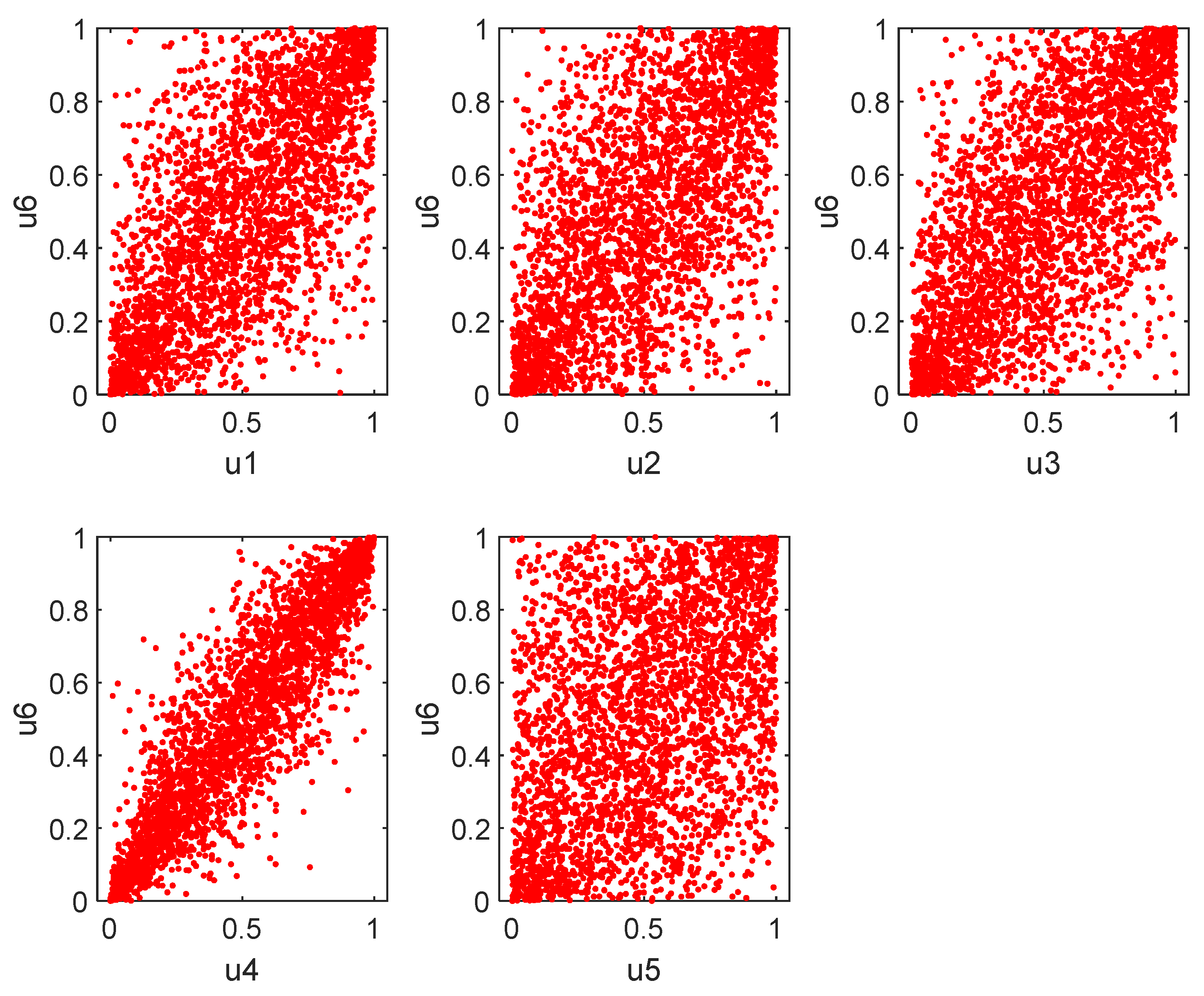
3.2. Marginal Distributions

We considered a group of GARCH models as candidates and find that the AR(1)-GJRGARCH(1,1) model developed by Glosten et al. (1993) is a suitable model for the marginal returns distributions based on the diagnostic tests for model adequacy (ARCH LM test and Ljung–Box test). Moreover, given the presence of large kurtosis in tails, we model the shock dynamics in both tails of each conditional distribution with a skewed student’s t distribution introduced by Hansen (1994). Thus, our choice is justified as the skewed Student’s t distribution can capture skewness and high kurtosis of series.
Table 3 below exhibits the results for the diagnostic tests for model adequacy.
Table 3 shows that the null hypothesis of no autocorrelation for the Ljung–Box test up to lag 30 is not rejected at 5% statistical level of significance because the p-values are greater than 0.05. As for the ARCH LM test up to lag 10, the null hypothesis of no heteroscedasticity is not rejected at 5% statistical level of significance because the p-values are greater than 0.05. Thus, the AR(1) GJR-GARCH (1,1) is a suitable model for our data.
Table 4 reports the parameters estimates from the AR(1) GJR-GARCH (1,1) model. We find that the sum of the GJR-GARCH parameters α 1 and β 1 is close to unity for all insurers indicating highly persistent volatilities. Moreover, we can see from the table that the leverage effect parameter γ is significant and positive at 5% confidence level for Discovery, Liberty, Sanlam, and Santam, except for Momentum, where it is negative and significant at 10%. A positive leverage effect implies that a negative return on the series increases volatility more than a positive return with the same magnitude.
Overall, the diagnostic test confirms that the marginal distribution used for this study is well-specified. Therefore, we can use the AR(1) GJR-GARCH (1,1) and the skewed t distribution alongside copulas to model the dependence structure.

3.3. Estimation of the Copula Models

This section focuses on the dependence between the market and the insurers. We first plot the scatter plots of the marginals between the market and each of the insurers. Figure 1 displays the joint behavior of extreme values between the marginals.
From the figure, there seems to be lower and upper tail dependence between the marginals. Hence, copula models that can account for both upper and lower tail dependence may be appropriate for the data.
In what follows, we estimate the dynamic mixture copula, namely the Rotated Clayton and Clayton (RC&C) and the Rotated Gumbel and Gumbel (RG&G), for each series, and the results of the estimations are reported in Table 5 and Table 6.
We can observe from Table 5 and Table 6 that the copula weights are between 0.392 and 0.485 for the RC&C (see Table 5) and between 0.555 and 0.696 for the RG&G (see Table 6). This provides strong evidence for an asymmetric dependence structure between insurers and the market.
Furthermore, we consider the symmetrized Joe-Clayton copula, which is a modification of the Joe-Clayton copula. Our interest in the symmetrized Joe-Clayton copula is its ability to measures the dependence in both the lower and upper tail. Hence, it possesses similar characteristics as the RC&C and RG&G copula models. Table 7 presents the estimation outputs of the bivariate time-varying Joe-Clayton copula between the market and each of the insurers.
Table 7 shows that the coefficient of the lower tail dependence ω L is significantly higher than the one of upper tail dependence ω U for three insurers except for Liberty and Santam. This behavior may suggest a lower tail dependence between Discovery, Momentum, Sanlam, and the market and an upper tail dependence between Liberty, Santam, and the market. Overall, the results display a dynamic and asymmetric dependence between the market and insurers.
Table 8 below shows the results of the log-likelihood function to select the best copula model.
Table 8 reports the estimated likelihood values for the tvSJC copula, the RC&C, and the RG&G. We can see that the mixture of the RG&G model has the lowest log-likelihood estimates for all insurers. Hence, it is a suitable copula model for the series than the other two copula models. Therefore, we use the RG&G to estimate the marginal expected shortfall of the five insurers.

3.4. Estimation of the DMC-MES

In this section, we use the estimates of the DMC-MES to establish a ranking for the contribution to systemic risk of the five insurers.
Table 9 provides the ranking of the five insurers based on the average DMC-MES. At the top of the list is Sanlam, the biggest insurer in South Africa, whose systemic risk measure is as high as 1.942, making Sanlam the systemically riskiest insurer in the South African insurance sector. Discovery which is among the biggest insurers in South Africa is the second-largest contributor to systemic risk with an average DMC-MES of 0.983. According to the literature, this might imply that Sanlam and Discovery are engaged in non-traditional business activities such as the issuance of Credit Default Swaps and securities lending, etc. In addition, our results indicate that financial institutions tend to be as systemically important as they are large.
Momentum Metropolitan and Liberty are next in the ranking, with an average DMC-MES of 0.805 and 0.583, respectively. On the other hand, Santam is the least systemically risky insurer in South Africa, with an average DMC-MES being negative −0.007. This implies that Santam is relatively resilient when the insurance market is in distress. This might indicate that Santam is still probably involved in traditional insurance business activities.

3.5. Robustness Test

3.5.1. Bivariate Copula

After filtering the data using AR(1)-GJRGARCH(1,1) models, the obtained pair of innovations (standardized residuals) was transformed to uniforms using the estimated skew Student-t distributions. The uniform series will be used as input for the bivariate Clayton and Gumbel copula to get an insight into the dependence structure between the largest contributor to systemic risk, Sanlam, and the market, and the other insurers.
The estimated parameters corresponding to each copula, the confidence interval (CI), the Akaike Information Criteria (AIC), and the Bayesian Information Criteria (BIC) values are reported in Table 10.
First, we can notice from the table that the Gumbel copula provides the best fit to the data between Sanlam, and Discovery, and Sanlam and Santam, since it has the lowest values for the AIC criteria. This indicates a greater dependence in the positive tail than in the negative. In other words, large gains from Sanlam and Discover; and Sanlam and Santam are more likely to occur simultaneously than large losses.
On the other hand, according to the AIC criteria, Table 10 tells us that the Clayton copula provides the best fit to the data between Sanlam and Liberty, Sanlam and Momentum Metropolitan, and Sanlam and the market, exhibiting greater dependence in the negative tail than in the positive. This means that large losses from Sanlam and Liberty, Sanlam and Momentum Metropolitan, and Sanlam and the market are more likely to happen simultaneously than a large gain. This finding is in line with our previous results as we expect a left tail dependence between Sanlam and the market.

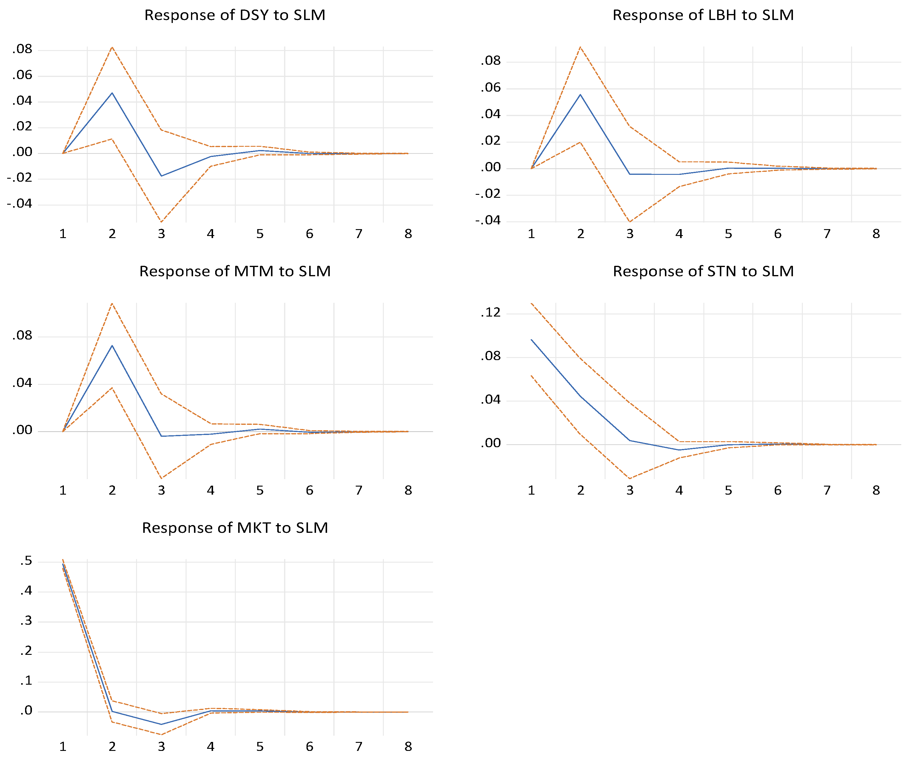
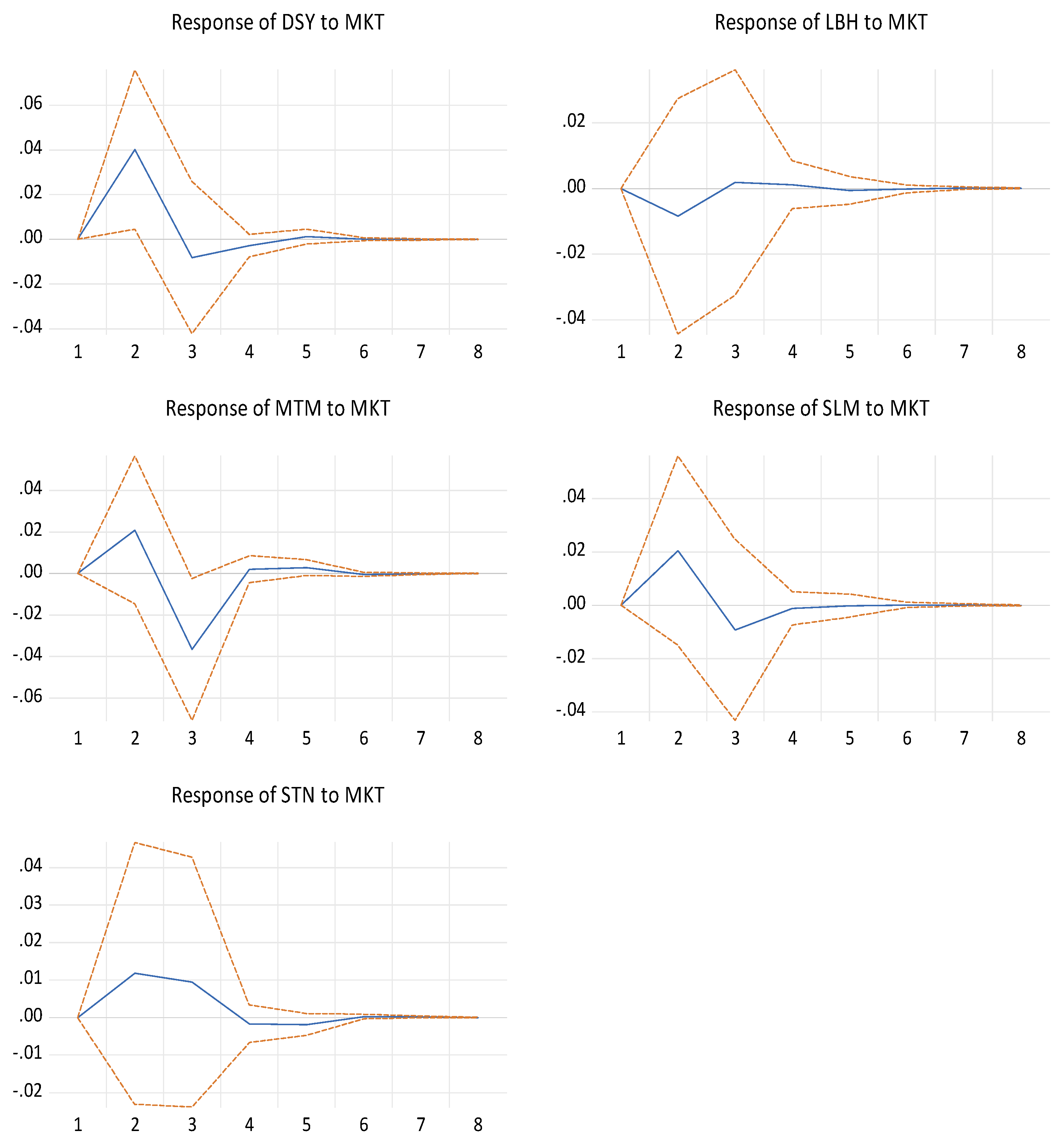
3.5.2. Impulse Response Function

In this section, we estimate a bivariate VAR model to determine the effect of a shock to Sanlam on the market and the other insurers; and to also determine the effect of a shock to the market on the five insurers. We use the Cholesky decomposition to orthogonalize the innovation shocks.
Figure 2 exhibits the impulse response of Sanlam to the market and the other insurers, while Figure 3 shows the impulse response of the market to the five insurers.
From Figure 2, we can first notice an initial increase from periods 1 to 2 of Discovery, Liberty, and Momentum Metropolitan to a one standard deviation shock (innovation) to Sanlam. Afterward, between periods 2 and 3, there is a sharp decline in their responses; they become negative and increase from the negative region to the positive region until they hit the steady-state. Conversely, we can see a sharp decline of Santam and market to a one standard deviation shock (innovation) to Sanlam. They become negative and increase gradually until they reach the steady-state.
In conclusion, this result confirms our previous findings as we expect a shock to Sanlam to have an adverse effect on the market and the insurers in the short run.
From Figure 3, we can first observe an initial increase from periods 1 to 2 of Discovery, Momentum Metropolitan, Sanlam, and Santam to a one standard deviation shock (innovation) to the market. Afterward, between period 2 and 3, there is a sharp decline in their responses, they become negative and increases from the negative region to the positive region until they hit their steady-state, except for Santam, where, between period 2 to 3, there is a slight decline in the positive region and from period 3 to 4 it declines into the negative region. Afterward, it reaches the steady-state between period 4 and 5, and gradually increases and hit again the steady-state in the long run. Finally, we can see a decline of Liberty to the negative region from periods 1 to 2 to a one standard deviation shock (innovation) to the market. It gradually increases between periods 2 and 3 until the positive region where it reaches the steady-state in the long run.
In conclusion, our result support our previous findings as we expect a shock to the market to have a negative impact on the insurance companies in the short run except for Santam.

4. Conclusions

In this paper, a Dynamic Mixture Copula Marginal Expected Shortfall (DMC-MES) is applied to measure systemic risk for five insurance companies in South Africa. Many studies argue that a primary factor causing systemic risk is the dynamic and asymmetric dependence between financial institutions. For this reason, we employed three copula models that can measure dynamic and asymmetric dependence. We used two dynamic mixture copula models, namely the Rotated Clayton and Clayton and the Rotated Gumbel and Gumbel, and the time-varying Symmetrized Joe-Clayton copula. Then, we compared the goodness of fit of the different copula models based on their log-likelihood estimates. We found that the Rotated Gumbel and Gumbel had the lowest log-likelihood estimates for all the pair of series, making it a suitable copula model for our data.
Finally, we used the Rotated Gumbel and Gumbel to estimate the marginal expected shortfall of the five insurers. The main findings showed that Sanlam is the largest contributor to systemic risk over the sample period, followed by Discovery, and Santam turns out to be the least systemically risky insurer. Our findings may imply that Sanlam and Discovery are more likely to be involved in non-traditional insurance activities such as financial securities, Credit Default Swap, derivatives, and many others.
In addition, our results revealed that the contribution of insurers to systemic risk in South Africa is linked to the size of the insurer, as Sanlam and Discovery are among the largest insurers in South Africa. This may indicate that instability in the insurance sector is more likely to occur if one of these two insurers is in financial difficulty. Thus, our results confirm the assumption that “no financial institution should be too big to fail (TBTF)”. Therefore, our findings could help South African regulators to have a better understanding of the dynamic and asymmetric dependence between insurers and the market in order to handle adequately systemic risk in the insurance sector by taking stricter regulatory measures in the form of higher capital and loss absorbency requirements for systemically risky insurers.
Due to data availability, we could not use all of the South African insurance companies listed on the Johannesburg Stock Exchange in our analysis. A possible extension of our study would be to include more copula models as well as other segments of the financial system such as the banking sector, the hedge funds market, and the real estate market so that one can have a broader picture of the systemically riskiest financial sector in South Africa.
One could also be interested in conducting more research on non-core activities of insurers in South Africa and their systemic impact.

Author Contributions

The contribution of each author is as follows: Conceptualization, J.W.M.M.; methodology, J.W.M.M., and E.S.E.F.A.; software, E.S.E.F.A.; validation, J.W.M.M.; formal analysis, E.S.E.F.A.; investigation, J.W.M.M., and E.S.E.F.A.; resources, E.S.E.F.A.; data curation, E.S.E.F.A.; writing—original draft preparation, E.S.E.F.A.; writing—review and editing, J.W.M.M.; visualization, E.S.E.F.A.; supervision, J.W.M.M.; project administration, E.S.E.F.A.; funding acquisition, Not Applicable. All authors have read and agreed to the published version of the manuscript.

Funding

This research received no external funding.

Data Availability Statement

The dataset consisting of daily stock prices is taken from the I-net BFA Database available at: http://research.mcgregorbfa.com/Default.aspx. (accessed on 15 June 2020).

Conflicts of Interest

The authors declare no conflict of interest. The authors certify that they have no affiliations with or involvement in any organization or entity with any financial or non-financial interest in the subject matter or materials discussed in this manuscript.

References

  1. Acharya, Viral V., and Matthew Richardson. 2014. Is the Insurance Industry Systemically Risky? In Modernizing Insurance Regulation. Edited by John H. Biggs and Matthew P. Richardson. New York: John Wiley & Sons, pp. 151–79. [Google Scholar]
  2. Berdin, Elia, and Matteo Sottocornola. 2015. Insurance Activities and Systemic Risk. SAFE Working Paper No.121. Frankfurt: Goethe University. [Google Scholar]
  3. Bernal, Oscar, Jean-Yves Gnabo, and Gregory Guilmin. 2014. Assessing the Contribution of Banks, Insurance, and Other Financial Services to Systemic Risk. Journal of Banking and Finance 47: 270–87. [Google Scholar] [CrossRef]
  4. Bierth, Christopher, Felix Irresberger, and Gregor N. F. Weiß. 2015. Systemic Risk of Insurers Around the Globe. Journal of Banking and Finance 55: 232–45. [Google Scholar] [CrossRef]
  5. Blasques, Francisco, Siem Jan Koopman, and Andre Lucas. 2014a. Maximum Likelihood Estimation for Generalized Autoregressive Score Models. Tinbergen Institute Discussion Paper. Amsterdam: VU University Amsterdam and Tinbergen Institute. [Google Scholar]
  6. Blasques, Francisco, Siem Jan Koopman, and Andre Lucas. 2014b. Stationarity and Ergodicity of Univariate Generalized Autoregressive Score Processes. Electronic Journal of Statistics 8: 1088–112. [Google Scholar] [CrossRef]
  7. Cerrato, Mario, John Crosby, Minjoo Kim, and Yang Zhao. 2015. Correlated Defaults of UK Banks: Dynamics and Asymmetries. Working paper 2015-24. Glasgow: Business School-Economics, University of Glasgow. [Google Scholar]
  8. Creal, Drew, Siem Jan Koopman, and Andre Lucas. 2013. Generalized Autoregressive Score Models with Applications. Journal of Applied Econometrics 28: 777–95. [Google Scholar] [CrossRef] [Green Version]
  9. Drakos, Anastassios A, and Georgios Kouretas. 2015. Bank Ownership, Financial Segments, and the Measurement of Systemic Risk: An Application of CoVaR. International Review of Economics and Finance 40: 127–40. [Google Scholar] [CrossRef]
  10. Dungey, Mardi, Matteo Luciani, and David Veredas. 2014. The Emergence of Systemically Important Insurers. Econometric Modeling: Capital Markets Risk eJournal. [Google Scholar] [CrossRef] [Green Version]
  11. Eckernkemper, Tobias. 2018. Modeling Systemic Risk: Time-Varying Tail Dependence when Forecasting Marginal Expected Shortfall. Journal of Financial Econometrics 16: 63–117. [Google Scholar] [CrossRef]
  12. Eling, Martin, and David Antonius Pankoke. 2016. Systemic Risk in the Insurance Sector: A review and Direction for Future Research. Risk Management and Insurance Review 19: 249–84. [Google Scholar] [CrossRef] [Green Version]
  13. ECB, European Central Bank. 2013. Financial Stability Review. Frankfurt: European Central Bank. [Google Scholar]
  14. Glosten, Lawrence. R., Ravi Jagannathan, and David E. Runkle. 1993. On the Relation Between the Expected Value and the Volatility of Nominal Excess Return on Stocks. Journal of Finance 48: 1779–801. [Google Scholar] [CrossRef]
  15. Grace, Martin F. 2011. The Insurance Industry and Systemic Risk: Evidence and Discussion. Working Paper. Atlanta: Georgia State University. [Google Scholar]
  16. Hansen, Bruce E. 1994. Autoregressive Conditional Density Estimation. International Economic Review 35: 705–30. [Google Scholar] [CrossRef]
  17. IMF, International Monetary Fund. 2009. Global Financial Stability Report. Washington: International Monetary Fund. [Google Scholar]
  18. IISA, Insurance Institute of South Africa. 2016. Business unusual. Paper presented at 43rd Annual Insurance Conference, Rustenburg, South Africa, July 2016. [Google Scholar]
  19. Kaserer, Christoph, and Christian Klein. 2019. Systemic Risk in Financial Markets: How Systemically Important Are Insurers? Journal of Risk and Insurance 86: 729–59. [Google Scholar] [CrossRef]
  20. National Treasury of South Africa. 2011. A Safer Financial Sector to Serve South Africa Better. Pretoria: National Treasury. [Google Scholar]
  21. Sklar, A. 1959. Fonctions de Repartition a n Dimensions et Leurs Marges. Paris: Publications de l’Institut de Statistique de l’Universite de Paris, vol. 8, pp. 229–31. [Google Scholar]
  22. Weiß, Gregor N.F, and Janina Muhlnickel. 2014. Why do Some Insurers Become Systemically Relevant? Journal of Financial Stability 13: 95–117. [Google Scholar] [CrossRef]
Figure 1. Scatter plots of the marginals. Note that the horizontal axis represents the marginal of the insurers, while the vertical axis represents the marginal of the market.
Ijfs 09 00029 g001
Figure 2. Impulse response function: Response of the market and other insurers to Sanlam shock.
Ijfs 09 00029 g002
Figure 3. Impulse response function: Response of each insurer to the market shock.
Ijfs 09 00029 g003
Table 1. List of the Five South African Insurance Companies.
CompanySymbolSector
Discovery LimitedDSYLife Insurance
Liberty Holdings LimitedLBHLife Insurance
Momentum Metropolitan HoldingsMTMLife Insurance
Sanlam LimitedSLMLife Insurance
Santam LimitedSNTNonlife Insurance
Table 2. Descriptive Statistics.
DiscoveryLibertyMomentumSanlamSantam
Mean0.041−0.0050.0050.030.026
Std.Dev.1.9571.8921.8681.9591.712
Skewness−0.5270.129−0132−0.429−0.474
Kurtosis12.69517.8537.1837.70314.13
JB test p-value0.0010.0010.0010.0010.001
Note: Table 2 reports descriptive statistics of the five insurers’ stock returns. JB test p-value is the probability that the returns are normally distributed, according to Jarque–Bera normality test. The sample period is from 13 November 2007 to 15 June 2020.
Table 3. Diagnostic Tests for Model Adequacy.
ModelLjung–Box Test Arch LM Test
DiscoveryAR(1)-GJRGARCH(1,1)Standardized residuals
Standardized squared residuals
0.4106
0.06036
0.3931
LibertyAR(1)-GJRGARCH(1,1)Standardized residuals
Standardized squared residuals
0.4117
0.2674
0.8041
MomentumAR(1)-GJRGARCH(1,1)Standardized residuals
Standardized squared residuals
0.1185
0.0823
0.6793
SanlamAR(1)-GJRGARCH(1,1)Standardized residuals
Standardized squared residuals
0.6952
0.7390
0.5538
SantamAR(1)-GJRGARCH(1,1)Standardized residuals
Standardized squared residuals
0.9213
0.7559
0.5491
MarketAR(1)-GJRGARCH(1,1)Standardized residuals
Standardized squared residuals
0.31172
0.4614
0.4527
Note: Table 3 reports insignificant Ljung—Box diagnostic test at 5% statistical significance level.
Table 4. Estimates of AR(1) GJR-GARCH (1,1) for Each Series.
AR (1)GJR-GARCH (1,1)Kurtosis Skewness
α 0 β 0 ω α 1 β 1 γ
Discovery0.0476
(0.0252)
−0.0058
(0.0183)
0.0385 ***
(0.0115)
0.0517 ***
(0.0126)
0.9058 ***
(0.0133)
0.0669 ***
(0.0182)
4.9419 ***
(1.571)
−0.2145 ***
(0.0259)
Liberty0.0159
(0.0251)
−0.0664 ***
(0.0165)
0.0366 ***
(0.0054)
0.0001
(0.0036)
0.9573 ***
(0.0024)
0.0603 ***
(0.0024)
12.32 ***
(0.330)
−0.0801 ***
(0.0246)
Momentum0.0321
(0.0263)
−0.0683 ***
(0.0181)
0.0567 ***
(0.0214)
0.0564 ***
(0.0173)
0.9138 ***
(0.0191)
−0.0318 *
(0.0171)
8.3628 ***
(0.9165)
0.0101 ***
(0.0027)
Sanlam0.0221
(0.0259)
−0.0690 ***
(0.0180)
0.0526 ***
(0.0154)
0.0353 ***
(0.0123)
0.9098 ***
(0.0138)
0.0849 ***
(0.0182)
4.7317 ***
(1.3719)
−0.1677 ***
(0.0153)
Santam0.0299
(0.0242)
−0.1172 ***
(0.0182)
0.4707 ***
(0.1510)
0.2065 ***
(0.0048)
0.6849 ***
(0.0737)
0.0292***
(0.0046)
16.038 ***
(2.195)
−0.6265 **
(0.249)
Note: Table 4 reports the estimated coefficients of the univariate AR (1) and GJR-GARCH (1,1) model. *, **, and *** represents statistical significance at 10%, 5%, and 1% respectively. standard errors are reported in ().
Table 5. Estimation Results of the Dynamic Mixture Copula of the Rotated Clayton and Clayton (RC&C): Between Market and Insurers.
WeightGAS (1,1)
w ˜ w 1 w 2 A 11 A 22 B 11 B 22
Discovery0.392 ***
(0.031)
0.109 ***
(0.078)
0.002 ***
(0.0001)
0.233 **
(0.118)
0.012 ***
(0.004)
0.849 ***
(0.107)
0.998 ***
(0.002)
Liberty0.485 ***
(0.039)
0.0005 ***
(0.00001)
0.0206
(0.021)
0.036 ***
(0.009)
0.136
(0.097)
0.998 ***
(0.004)
0.959 ***
(0.045)
Momentum0.463 ***
(0.065)
−0.003 ***
(0.0001)
0.007 ***
(0.0001)
0.067
(0.104)
0.023 ***
(0.0012)
1.003 ***
(0.0001)
0.989 ***
(0.0004)
Sanlam0.347 ***
(0.029)
−0.002 ***
(0.0001)
−0.001 ***
(0.0005)
0.011
(0.012)
0.044 ***
(0.008)
1.0014 ***
(0.0001)
1.0013 ***
(0.0003)
Santam0.423 ***
(0.057)
−0.002(
0.004)
0.0001
(0.0004)
0.094
(0.09)
0.034
(0.041)
0.995 ***
(0.011)
0.998 ***
(0.003)
Note: Table 5 reports the estimated dynamic mixture copula weights for the rotated Clayton and Clayton copula models (RC&C). **, and *** represents statistical significance at 5%, and 1% significance level respectively. Standard errors are reported in ().
Table 6. Estimation Results of Dynamic Mixture Copula of the Rotated Gumbel and Gumbel (RG&G): Between Markets and Insurers.
WeightGAS (1,1)
w ˜ w 1 w 2 A 11 A 22 B 11 B 22
Discovery0.639 ***
(0.044)
−0.006
(0.026)
0.082
(0.113)
0.144 ***
(0.093)
0.175
(0.235)
0.659 ***
(0.221)
0.539
(0.606)
Liberty0.555 ***
(0.049)
−0.132
(0.105)
−0.327
(0.241)
0.229
(0.159)
−0.175
(0.227)
0.497
(0.329)
0.394
(0.641)
Momentum0.567 ***
(0.0009)
−0.0006 ***
(0.00001)
−0.002 **
(0.0001)
−0.017 ***
(0.0001)
0.048 **
(0.003)
1.0004 ***
(0.0001)
0.991 ***
(0.0004)
Sanlam0.696 ***
(0.045)
0.019 ***
(0.009)
0.039
(0.029)
0.032 **
(0.012)
−0.154
(0.114)
0.982 ***
(0.009)
0.961 ***
(0.029)
Santam0.643 ***
(0.086)
−0.003
(0.006)
−1.212 **
(0.524)
0.042
(0.047)
2.159
(1.528)
0.996 ***
(0.007)
0.948 ***
(0.316)
Note: Table 6 reports the estimated dynamic mixture copula weights for the rotated Gumbel and Gumbel copula models (RG&G). **, and *** represents statistical significance level at 5%, and 1% respectively. Standard errors are reported in ().
Table 7. Estimation Output of the Time-Varying SJC copula.
Time-Varying SJC Copula
DiscoveryLibertyMomentumSanlamSantam
ω U 1.958
(1.58)
2.032 **
(0.96)
0.094 *
(0.05)
8.707
(23.14)
−0.040
(0.37)
α U −9.999
(8.21)
−9.969 **
(4.99)
−0.493 *
(0.28)
9.761 ***
(1.24)
−0.733
(0.84)
β U 0.431
(0.62)
−0.424
(0.64)
0.976 ***
(0.02)
4.477
(39.03)
0.832 ***
(0.25)
ω L 2.849 **
(1.41)
0.111 ***
(0.03)
2.944 ***
(0.48)
9.984 ***
(0.99)
−0.094
(0.39)
α L −9.999
(9.79)
−0.526 ***
(0.17)
−9.997 ***
(2.45)
9.889
(92.22)
−1.546
(1.95)
β L −0.040
(0.33)
0.974 ***
(0.01)
−0.647 ***
(0.13)
−9.796 ***
(2.15)
0.143
(0.34)
Note: Table 7 reports the estimated coefficients of the time-varying SJC copula model. *, **, and *** represents statistical significance at 10%, 5%, and 1% respectively. Standard errors are reported in ().
Table 8. Log-Likelihood Estimates.
CopulastvSJCRC&CRG&G
Copula Likelihood
Discovery−1115.9−1093.4−1117.8
Liberty−768.0−762.9−778.4
Momentum−910.7−903.3−925.6
Sanlam−2344.0−2693.7−2774.4
Santam−304.1−305.9−307.5
Table 9. Summary Statistics for DMC-MES for All Insurers Based on RG&G.
MeanStd.DevMinMaxRanking
Discovery0.9837.7090.0551334.39862
Liberty0.5835.7480.0375216.43424
Momentum0.8055.5800.0618223.89663
Sanlam1.94218.1320.1128894.16381
Santam−0.0070.100−2.34904.30395
Table 10. Parameters for the Copulas and Their 95% Confidence Intervals between Sanlam and the Market, and Sanlam and the Other Insurers.
CopulaParameters95% CIAICBIC
Gumbel(MKT)3.431[3.343, 3.519]5160.05170.0
Clayton(MKT)3.568[3.462, 3.673]4510.04520.0
Gumbel(DSY)1.450[1.412, 1.487]780.4786.4
Clayton(DSY)0.781[0.726, 0.837]802.1808.1
Gumbel(LBH)1.384[1.349, 1.419]617.6623.7
Clayton(LBH)0.636[0.582, 0.689]594.0600.1
Gumbel(MTM)1.455[1.418, 1.492]791.2797.2
Clayton(MTM)0.753[0.697, 0.808]765.3771.3
Gumbel(STN)1.775[1.149, 1.206]175.5181.6
Clayton(STN)0.354[0.305, 0.403]233.9240.0
Publisher’s Note: MDPI stays neutral with regard to jurisdictional claims in published maps and institutional affiliations.

