Hardware Implementation of a Softmax-Like Function for Deep Learning †


Electrical and Computer Engineering Department, University of Patras, 26 504 Patras, Greece
*
Author to whom correspondence should be addressed.
†
This paper is an extended version of our paper published in Proceedings of the 8th International Conference on Modern Circuits and Systems Technologies (MOCAST), Thessaloniki, Greece, 13–15 May 2019.
Technologies 2020, 8(3), 46; https://0-doi-org.brum.beds.ac.uk/10.3390/technologies8030046
Submission received: 28 April 2020
/
Revised: 14 August 2020
/
Accepted: 25 August 2020
/
Published: 28 August 2020
(This article belongs to the Special Issue MOCAST 2019: Modern Circuits and Systems Technologies on Electronics)
Abstract
:In this paper a simplified hardware implementation of a CNN softmax-like layer is proposed. Initially the softmax activation function is analyzed in terms of required numerical accuracy and certain optimizations are proposed. A proposed adaptable hardware architecture is evaluated in terms of the introduced error due to the proposed softmax-like function. The proposed architecture can be adopted to the accuracy required by the application by retaining or eliminating certain terms of the approximation thus allowing to explore accuracy for complexity trade-offs. Furthermore, the proposed circuits are synthesized in a 90 nm 1.0 V CMOS standard-cell library using Synopsys Design Compiler. Comparisons reveal that significant reduction is achieved in area × delay and power × delay products for certain cases, respectively, over prior art. Area and power savings are achieved with respect to performance and accuracy.
1. Introduction
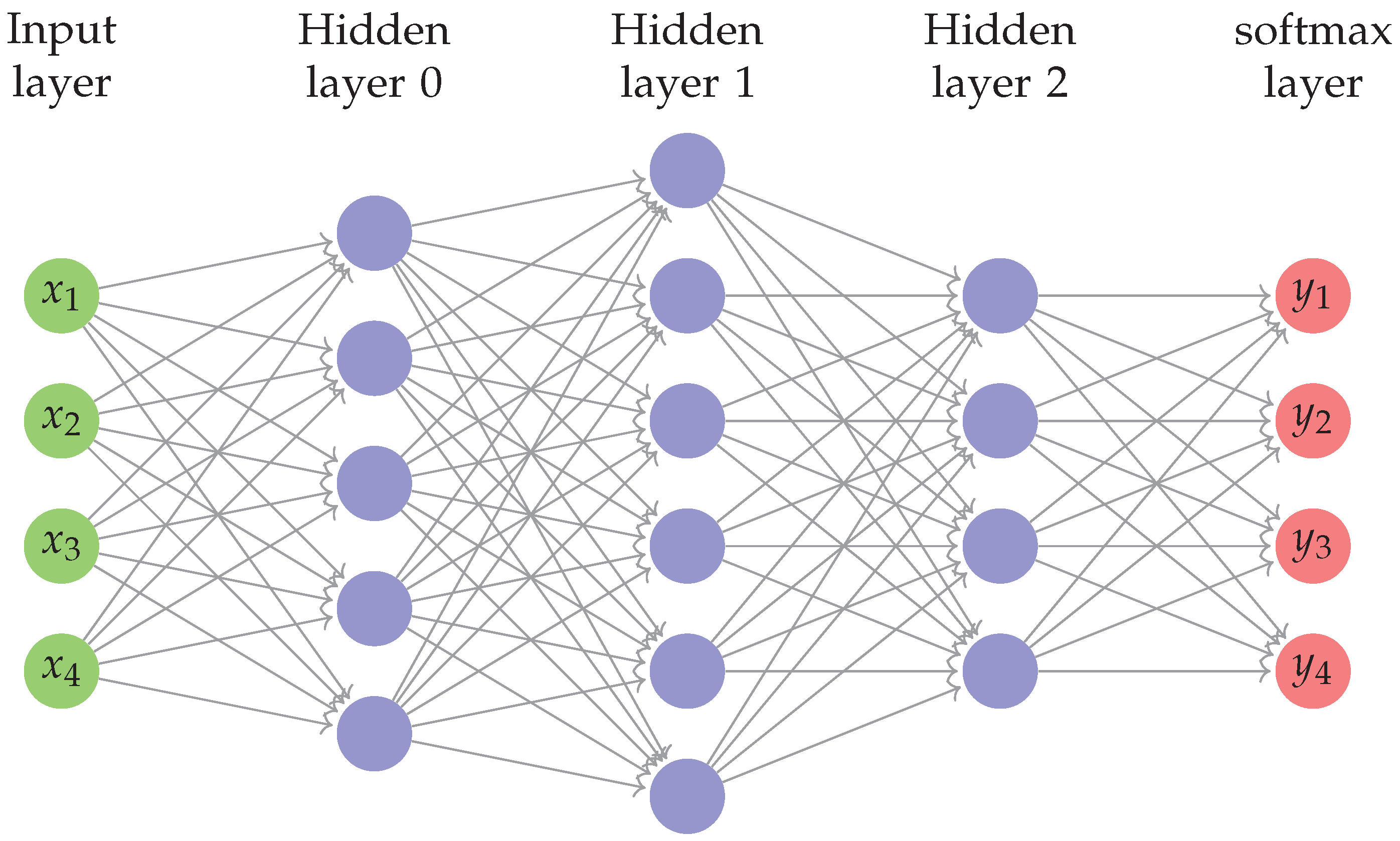
Deep neural networks (DNN) have emerged as a means to tackle complex problems such as image classification and speech recognition. The success of DNNs is attributed to the big data availability, the easy access to enormous computational power and the introduction of novel algorithms that have substantially improved the effectiveness of the training and inference [1]. A DNN is defined as a neural network (NN) which contains more than one hidden layer. In the literature, a graph is used to represent a DNN, with a set of nodes in each layer, as shown in Figure 1. The nodes at each layer are connected to the nodes of the subsequent layer. Each node performs processing including the computation of an activation function [2]. The extremely large number of nodes at each layer impels the training procedure to require extensive computational resources.
A class of DNNs are the convolutional neural networks (CNNs) [2]. CNNs offer high accuracy in computer-vision problems such as face recognition and video processing [3] and have been adopted in many modern applications. A typical CNN consists of several layers, each one of which can be convolutional, pooling, or normalization with the last one to be a non-linear activation function. A common choice for normalization layers is usually the softmax function as shown in Figure 1. To cope with increased computational load, several FPGA accelerators have been proposed and have demonstrated that convolutional layers exhibit the largest hardware complexity in a CNN [4,5,6,7,8,9,10,11,12,13,14,15]. In addition to CNNs, hardware accelerators for RNNs and LSTMs have also been investigated [16,17,18]. In order to implement a CNN in hardware, the softmax layer should also be implemented with low complexity. Furthermore, the hidden layers of a DNN can use the softmax function when the model is designed to choose one among several different options for some internal variable [2]. In particular, neural turing machines (NTM) [19] and differentiable neural computer (DNC) [20] use softmax layers within the neural network. Moreover, softmax is incorporated in attention mechanisms, an application of which is machine translation [21]. Furthermore, both hardware [22,23,24,25,26,27,28] and memory-optimized software [29,30] implementations of the softmax function have been proposed. This paper, extending previous work published in MOCAST2019 [31], proposes a simplified architecture for a softmax-like function, the hardware implementation of which is based on a proposed approximation which exploits the statistical structure of the vectors processed by the softmax layers in various CNNs. Compared to the previous work [31], this paper uses a large set of known CNNs, and performs extensive and fair experiments to study the impact of the applied optimizations in terms of the achieved accuracy. Moreover the architecture in [31] is further elaborated and generalized by taking into account the requirements of the targeted application. Finally, the proposed architecture is compared with various softmax hardware implementations. In order for the softmax-like function to be implemented efficiently in hardware, the approximation requirements are relaxed.
The remainder of the paper is organized as follows. Section 2 revisits the softmax activation function. Section 3 describes the proposed algorithm and Section 4 offers a quantitative analysis of the proposed architecture. Section 5 discusses the hardware complexity of the proposed scheme based on synthesis results. Finally, conclusions are summarized in Section 6.
2. Softmax Layer Review
CNNs consist of a number of stages each of which contains several layers. The final layer is usually fully-connected using ReLU as an activation function and drives a softmax layer before the final output of the CNN. The classification performed by the CNNs is accomplished at the final layer of the network. In particular, for a CNN which consists of layers, the softmax function is used to transform the real values generated by the th CNN layer to possibilities, according to
where is an arbitrary vector with real values , , generated at the th layer of the CNN and is the size of the vector. The ()st layer is called the softmax layer. By applying the logarithm function to both sides of (1), it follows that
The next section presents the proposed simplifications for (16) and the derivative architecture for the softmax-like hardware implementation.
3. Proposed Softmax Architecture
Equation (15) involves the distance of the maximum component from the remainder of the components of a vector. As , the differences in s increase and . On the contrary, as the differences in s are eliminated. Based on this observation, a simplifying approximation can be obtained, as follows. The third term in the right hand side of (16), , can be roughly approximated by 0. Hence, (16) is approximated by
Furthermore, this simplification substantially reduces hardware complexity as described below. From (17), it follows that
Proof.
Due to the softmax definition, it holds that
Corollary 1.
It holds that
Proof.
Proof is trivial and is omitted. □
Theorem 1 states that the proposed softmax-like function and the actual softmax function always derive the same decisions. The proposed softmax-like approximation is based on the idea that the softmax function is used during training to target an output by using maximum-log likelihood [2]. Hence, if the correct answer has already the maximum input value to the softmax function then will roughly alter the output decision due to the exponent function used in term . In general, , since the sequence cannot be denoted as a probability density function. For models where the normalization function is required to be a pdf, a modified approach can be followed, as detailed below.
According to the second approach, from (11) and (12) it follows:
with , where are chosen to be the top maximum values of . For the quantity , it holds , with being the remainder values of the vector , i.e., .
Equation (30) uses parameter which defines the number of additional terms used. By properly selecting , then it holds that and (30) approximates pdf better than (18). This is derived from the fact that in a real life CNN, the maximum values are those that contribute to the computation of the softmax since all the remainder values are close to zero.
Lemma 1.
It holds when
Proof.
By definition, it holds that when then , since the maximum value is identified as the maximum . Hence, by substituting in (30), it derives that
□
From a hardware perspective, (18) and (30) can be performed by the same circuit which implements the exponential function. The contributions of the paper are as follows. Firstly, the quantity is eliminated from (16), implying that the target application requires decision making. Secondly, further mathematical manipulations are proposed to be applied to (30), in order to approximate the outputs as pdf i.e., probabilities that sum to one. Thirdly, the circuit for the evaluation of is simplified, since
and
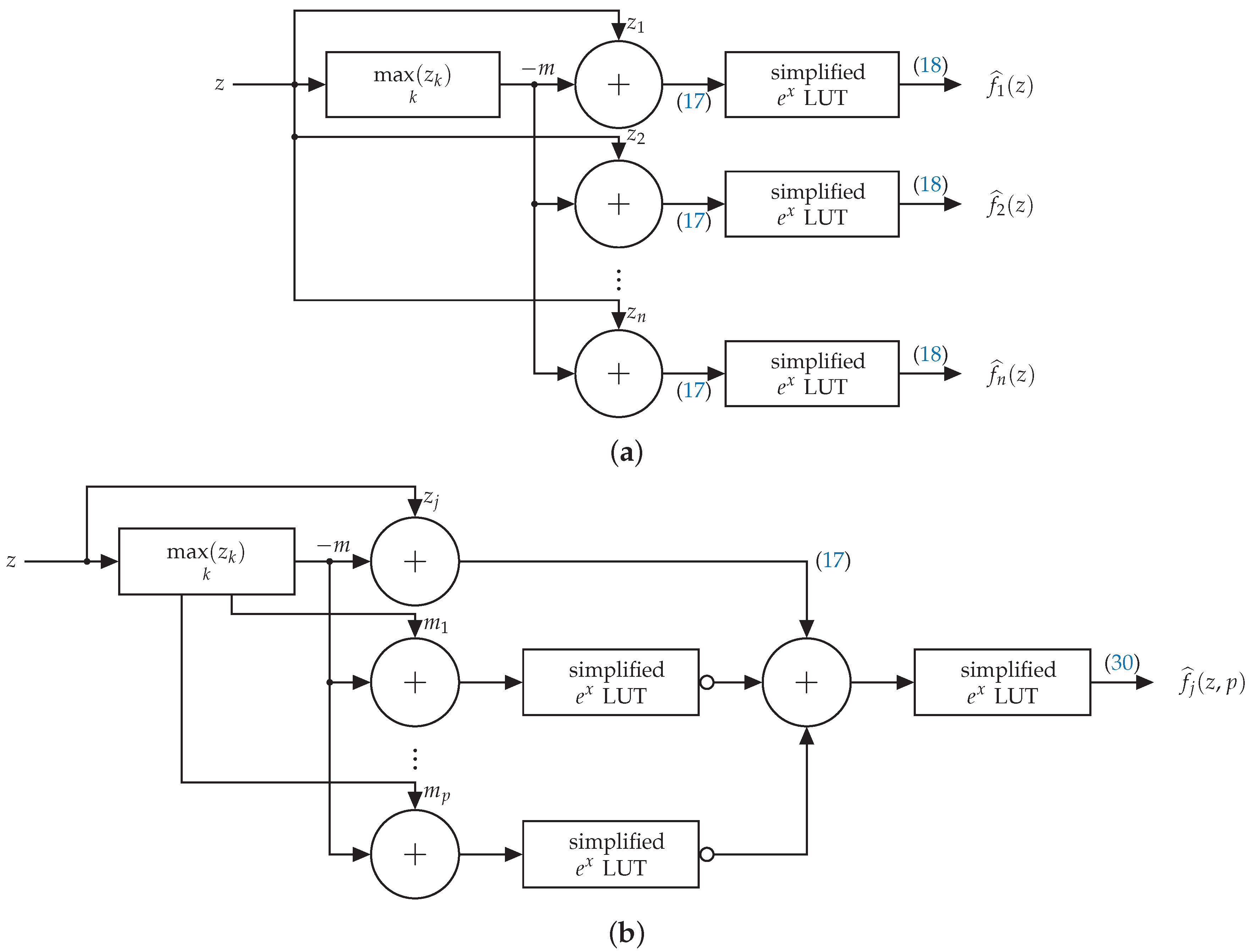
Figure 2 depicts the various building blocks of the proposed architecture. More specifically, the proposed architecture is comprised of the block which computes the maximum , i.e., . The particular computation is performed by a tree which generates the maximum by comparing the elements by two, as shown in Figure 3. The depicted tree structure generates , . Notation denotes the maximum of and , while denotes the maximum of and . The same architecture is used to compute the top maximum values of s. For example, , , and are the top four maximum values and is the maximum.
Subsequently, is subtracted from all the component values as dictated by (17). The subtraction is performed through adders, denoted as in Figure 2, using two’s complement representation for the input negative values . The obtained differences, also represented in two’s complement, are used as inputs to a LUT, which performs the proposed simplified operation of (18), to compute the final vector as shown in Figure 2a. Additional terms are added and subsequently each output through (30) generates the final value for the softmax-like layer output as shown in Figure 2b. For the hardware implementation of the function, an LUT is adopted the input of which is . The LUT size increases on the larger range of . Our proposed hardware implementation is simpler than other exponential implementations which propose CORDIC transformations [32], use floating-point representation [33], or LUTs [34]. In (33), the values are restricted to the range and the derived LUT size significantly diminishes and leads to simplified hardware implementation. Furthermore, no conversion from the logarithmic to the linear domain is required, since represents the final classification layer.
The next section quantitatively investigates the validity and usefulness of employing , in terms of the approximation error.
4. Quantitative Analysis of Introduced Error
This section quantitatively verifies the applicability of the approximation introduced in Section 2, for certain applications, by means of a series of Examples.
In order to quantify the error introduced by the proposed architecture, the mean square error (MSE) is evaluated as
where and are the expected and the actually evaluated softmax output, respectively.
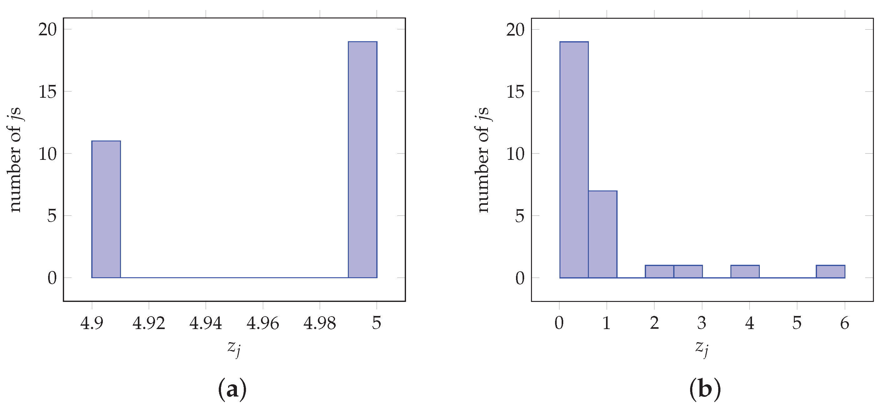
As an illustrative example, denoted as Example 1, Figure 4 depicts the histograms of component values in test vectors used as inputs to the proposed architecture, selected to have specific properties detailed below. The corresponding parameters are evaluated by using the proposed architecture for the case of a 10-bit fixed-point representation, where 5 bits are used for the integer and 5 bits are allocated to the fractional part. More specifically, the vector in Figure 4a contains values, for which it holds that , and . For this case the softmax values obtained by (1) are
From a CNN perspective, the softmax layer output generates similar values, where possibilities are all around 3%, and hence classification or decision cannot be made with high confidence. By using (18), the modified softmax values are
The statistical structure of the vector is characterized by the quantity of (15). The estimated dictates that the particular vector is not suitable as an alternative to softmax input in terms of CNN performance, i.e., the obtained classification is performed with low confidence. Hence although the proposed approximation in (18) demonstrates large differences when compared to (1), neither is applicable in CNN terms.
Consider the following Example 2. The component values for vector in Example 2 are
the histogram of which is shown in Figure 4b. In this case, the statistical structure of the vector demonstrates and . The feature of vector in Example 2 is that it contains three large different component values close to each other, namely and all other components are smaller than 1. The softmax output in (1) for the values in the particular are
By using the proposed approximation (18), the obtained modified softmax values are
Equations (41) and (42) show that the proposed architecture chooses component with value 1 while the actual probability is 0.7675. This means that the introduced error of can be negligible depending on the application, dictated by .
In the following, tests using vectors obtained from real CNN applications are considered. More specifically, in an example shown in Figure 5, the vectors are obtained from image and digit classification applications. In particular, Figure 5a,b depict the values used as input to the final softmax layer, generated during a single inference for a VGG-16 imagenet image classification network for 1000 classes and a custom net for MNIST digit classification for 10 classes. Quantity can be used to determine whether the proposed architecture is appropriate for application on vector before evaluating the MSE. It is noted that for the example of Figure 5a and for the example of Figure 5b are of the orders of and , respectively which renders them as negligible.
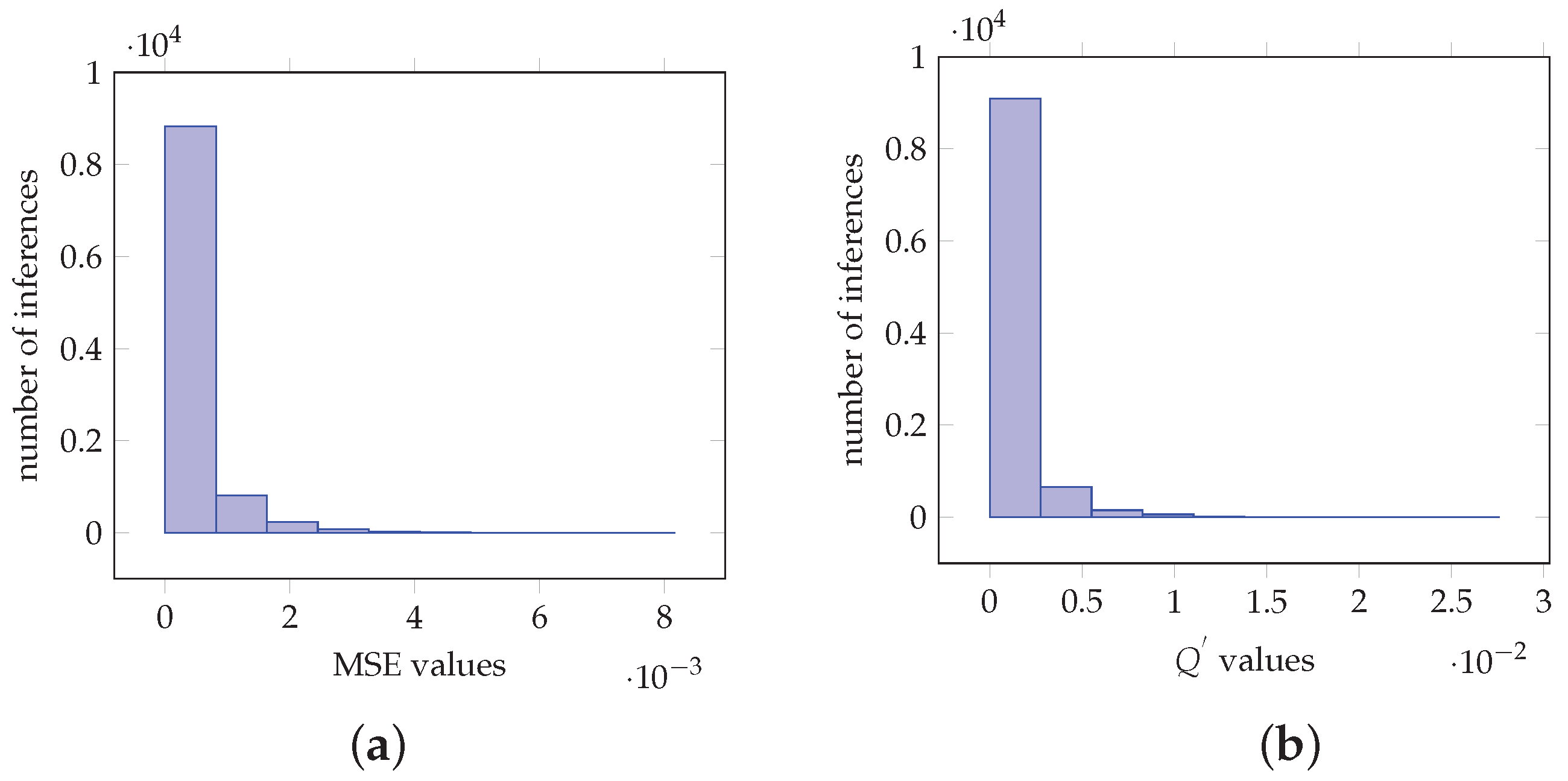
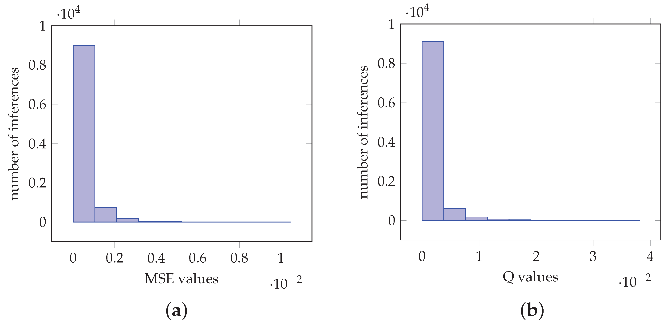
Subsequently, the proposed method is applied on the ResNet-50 [35], VGG-16, VGG-19 [36], InceptionV3 [37] and MobileNetV2 [38] CNNs, for 1000 classes with 10000 inferences of a custom image data set. In particular, for the case of ResNet-50, Figure 6a,b depict the histograms of the MSE and values, respectively. More specifically, Figure 6a demonstrates that the MSE values are of magnitude with 8828 of the values be in the interval. Furthermore, Figure 6b shows that the values are of magnitude with 9096 of them be in the interval . Furthermore, Table 1a–e depict actual softmax and the proposed method softmax-like values obtained by executing inference on the CNN models for six custom images. The values are sorted from left to right with the maximum value on the left side. Furthermore, the inferences and denote the same custom image as input to the model. More specifically, Table 1a demonstrates values from six inferences for the ResNet-50 model. It is shown that for the case of inference the maximum obtained values are and , for and , respectively. Other values are , , , and , , , , respectively. Hence, as shown by colorally 1, the maximum takes the value ‘1’ and the remainder of the values follow the values obtained by the actual softmax function. Similar analysis can be obtained for all the inferences and for each one of the CNNs. Furthermore, the same class is outputted from the CNN in both cases for each inference.
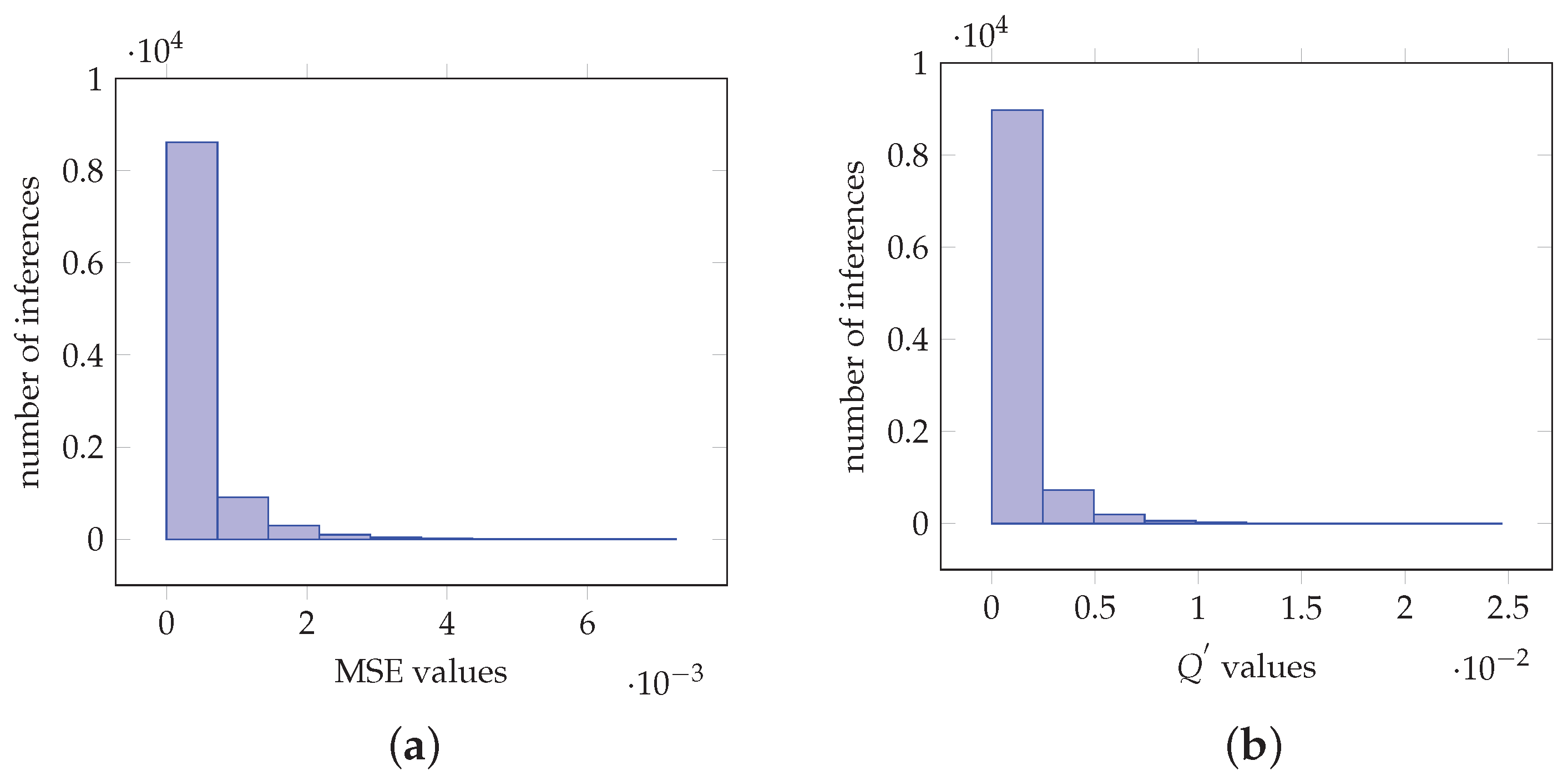
For the case of VGG-16, Figure 7a depicts the histogram of the MSE values. It is shown that the values are of magnitude and 8616 are in the interval . Figure 7b demonstrates histogram for the values with magnitude of and more than 8978 values are in the interval . Table 1b demonstrates that in the case of the and inference the top values are 0.51182884 and 1, respectively. The second top values are 0.18920843 and 0.369140625, respectively. In this case, the decision is made with a confidence of 0.51182884 for the actual softmax value and 1 for the softmax-like value. Furthermore, the second top value is 0.369140625 which is not negligible when compared to 1 and hence denotes that the selected class is of low confidence. The same conclusion derives for the case of the actual softmax value. Furthermore, for the case of and inferences, the values obtained by Figure 8b are close to the actual pdf softmax outputs. In particular, for the and cases, the top 5 values are 0.747070313, 0.10941570, 0.065981410, 0.018329350, 0.012467328 and 0.747070313, 0.110351563, 0.06640625, 0.017578125, 0.01171875, respectively. It is shown that values are similar. Hence, depending the application, an alternative architecture, as shown in Figure 2b can be used to generate pdf softmax values as outputs.
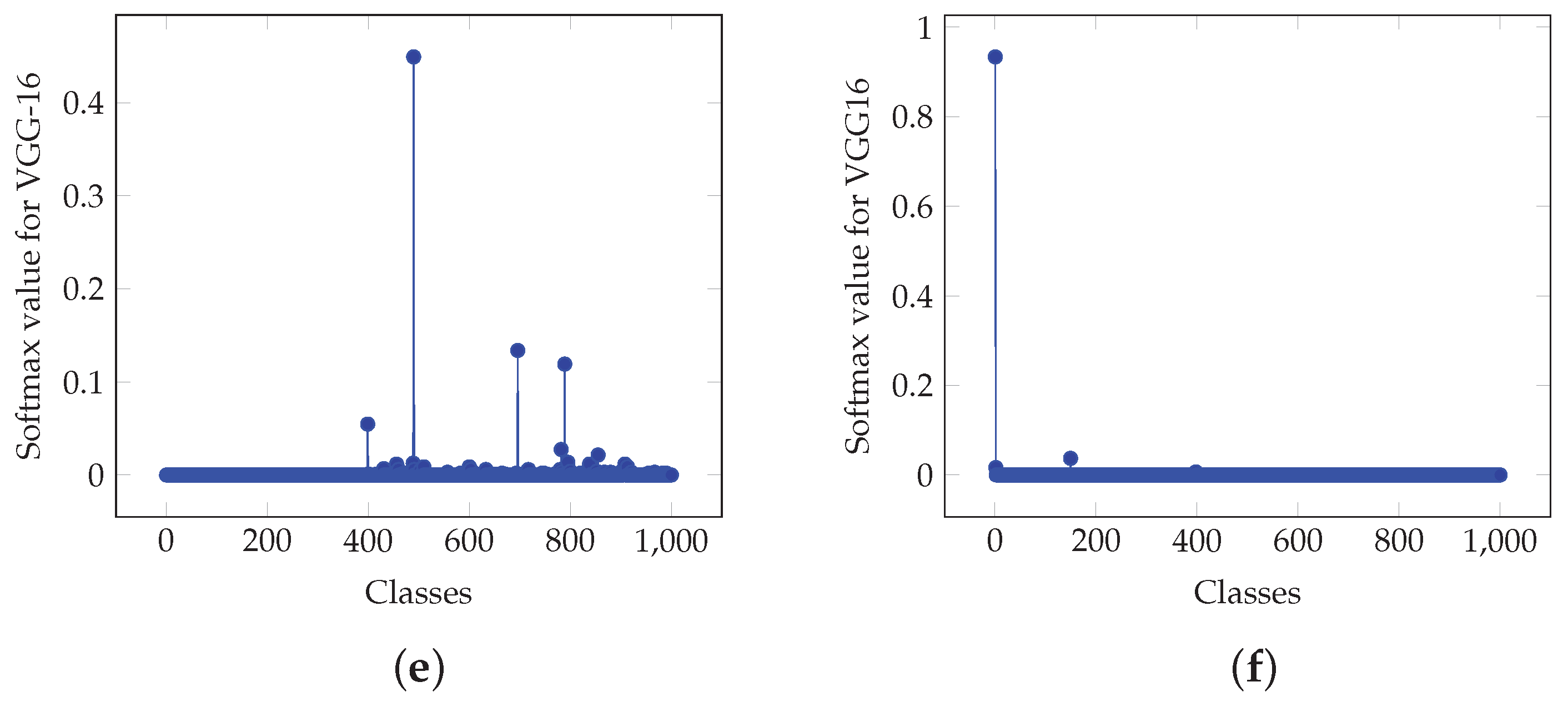
Moreover, Figure 8a,b depict graphically the values for the actual softmax and the proposed softmax-like output for inferences A and B, respectively, for the case of the VGG-16 CNN for the output classification. Furthermore, Figure 8c–f depict values for the architectures in Figure 2a,b, respectively. It is shown that in the case of Figure 2a, the values demonstrate a similar structure. In case of Figure 2b, values are similar to the actual softmax outputs.
Similar analysis can be performed for the case of VGG-19. In particular, Figure 9a demonstrates that MSE is of magnitude and 8351 of which are in the interval . In Figure 9b 8380 values are in the interval . For the case of InceptionV3, histograms in Figure 10a,b demonstrate MSE and values the 9194 and 9463 of which are in the intervals and , respectively. For the MobileNetV2 network, Figure 11a,b demonstrate MSE and values the 8990 and 9103 of which are in the intervals and , respectively. Furthermore, Table 1c–e derive similar conclusions as in the case of VGG-16.
In general, in all cases identical output decisions are obtained for the actual softmax and the softmax-like output layer for each one of the CNNs.
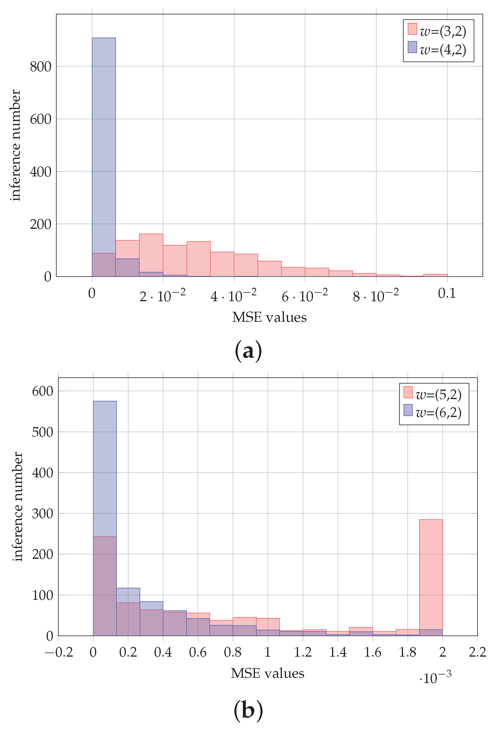
Considering the impact of the data wordlegth representation, let denote the fixed-point representation of a number with integral and fractional bits. Figure 12a,b depict histograms for the MSE values obtained for the case of 1000 inferences by the VGG-16 CNN. It is shown that the case demonstrates the smaller MSE values. The reason for this is that the maximum value of the inputs in the softmax layer is 56 for all the 1000 inferences, and hence the value of 6 for the integral part is sufficient.
Summarizing, it is shown that the proposed architecture suits well for the final stage of a CNN network as an alternative to implementing the softmax layer stage, since the MSE is negligible. Next, the proposed architecture is implemented in hardware and compared with published counterparts.
5. Hardware Implementation Results
This section describes implementation results obtained by synthesizing the proposed architecture outlined in Figure 2. Among several authors reporting results on CNN accelerators, [22,23,24] have recently published works focusing on hardware implementation of the softmax function. In particular, in [23], a study based on stochastic computation is presented. Geng et al. provide a framework for the design and optimization of softmax implementation in hardware [26]. They also discuss operand bit-width minimization, taking into account application accuracy constraints. Du et al. propose a hardware architecture that derives the softmax function without a divider [25]. The appproach relies on an equivalent softmax expression which requires natural logarithms and exponentials. They provide detailed evaluation of the impact of the particular implementation on several benchmarks. Li et al. describe a 16-bit fixed-point hardware implementation of the softmax function [27]. They use a combination of look-up tables and multi-segment linear approximations for the approximation of exponentials and a radix-4 Booth–Wallace-based 6-stage pipeline multiplier and modified shift-compare divider.
In [24], the architecture demonstrates LUT-based computations that add complexity and exhibits 444,858 m area complexity by using 65-nm standard-cell library. For the same library the architecture in [25] reports 640,000 m area complexity with 0.8 w power consumption at a 500 MHz clock frequency. The architecture in [28] reports 104,526 m area complexity with 4.24 w power consumption at a 1 GHz clock frequency. The proposed architecture in [26] demonstrates power consumption and area complexity of 1.8 w and 3000 m, respectively at a 500 MHz clock frequency with UMC 65 nm standard cell library. In [27], it is reported 3.3 GHz and 34,348 m frequency and area complexity at 45 nm technology node. Yuan [22] presented an architecture for implementing the softmax layer. Nevertheless there is no discussion of the implementation of the LUTs and there are no synthesis results. Our proposed softmax-like function differs from the actual softmax function due to the approximation of the quantity , as discussed in Section 3. In particular, (18) approximates the softmax output as a decision making application and not as a pdf function. The proposed softmax-like function in (30) approximates outputs as pdf function, depending on the number of terms used. As , (30) actual softmax function. The hardware complexity reduction derives from the fact that a limited number, , of s contribute to the computation of the softmax function. Summarizing, we compare both architectures depicted in Figure 2a,b with [22] to quantify the impact of on the hardware complexity. Section 4 shows that the softmax-like function suits well in a CNN. For a fair comparison we have implemented and synthesized both architectures, our proposed and [22], by using a 90 nm 1.0 V CMOS standard-cell library with Synopsys Design Compiler [39].
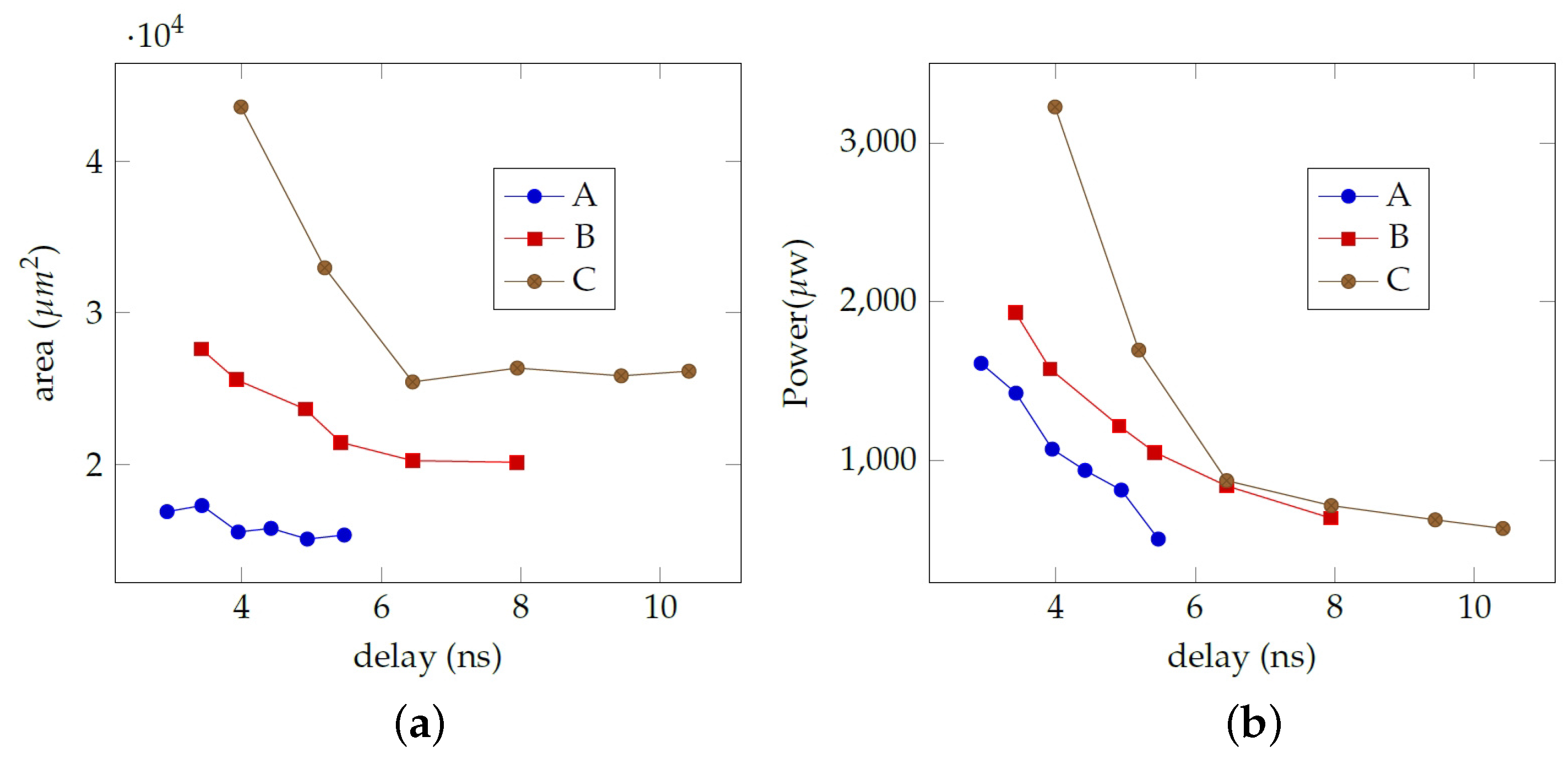
Figure 13 depicts the architecture obtained from synthesis where the various building blocks, namely maximum evaluation, subtractor and the simplified exponential LUTs that perform in parallel, are shown. Furthermore registers have been added at the circuits inputs and outputs for applying the delay constraints. Detailed results are depicted in Table 2a–c for the proposed softmax-like of Figure 2a, the [22] and the proposed softmax-like of Figure 2b layer with size 10, respectively. Furthermore, results are plotted graphically in Figure 14a,b where area vs. delay and power vs. delay are depicted, respectively. Results demonstrate that substantially area savings are achieved with no delay penalty. More specifically, for a 4 ns delay constraint the area complexity is 25,597 m and 43,576 m in case of architectures in Figure 2b and [22], respectively. For the case where the pdf output is not significant, the area complexity reduction can be 17,293 m for the architecture on Figure 2a. Summarizing, depending on the application and the design constraints there is a trade-off between the additional terms used for the evaluation of the softmax output. As we increase the value of the parameter , then the actual softmax value is better approximated while hardware complexity increases. When , then the hardware complexity is minimized while softmax output approximation diverges.
6. Conclusions
This paper proposes hardware architectures for implementing the softmax layer in a CNN with substantially reduced reduction in and product, respectively, for certain cases. A family of architectures that can approximate the softmax function have been introduced and evaluated, each member of which is obtained through a design parameter , which controls the number of terms employed for the approximation. It is found that a very simple approximation using , suffices to deliver accurate results in certain cases, even though the derived approximation is not a pdf. Furthermore, it has been demonstrated that for image and digit classification applications, the proposed architecture suits ideally as it achieves MSEs of the order of and , respectively, which are considered low.
Author Contributions
All authors contributed equally. All authors have read and agreed to the published verion of the manuscript.
Funding
This research received no external funding.
Conflicts of Interest
The authors declare no conflict of interest.
References
- LeCun, Y.; Bengio, Y.; Hinton, G. Deep learning. Nature 2015, 521, 436–444. [Google Scholar] [CrossRef] [PubMed]
- Goodfellow, I.; Bengio, Y.; Courville, A. Deep Learning; MIT Press: Cambridge, MA, USA, 2016; Available online: http://www.deeplearningbook.org (accessed on 27 August 2020).
- Girshick, R.B.; Donahue, J.; Darrell, T.; Malik, J. Rich feature hierarchies for accurate object detection and semantic segmentation. In Proceedings of the IEEE Conference on Computer Vision and Pattern Recognition, Columbus, OH, USA, 23–28 June 2014. [Google Scholar]
- Carreras, M.; Deriu, G.; Meloni, P. Flexible Acceleration of Convolutions on FPGAs: NEURAghe 2.0; Ph.D. Workshop; CPS Summer School: Alghero, Italy, 23 September 2019. [Google Scholar]
- Zainab, M.; Usmani, A.R.; Mehrban, S.; Hussain, M. FPGA Based Implementations of RNN and CNN: A Brief Analysis. In Proceedings of the 2019 International Conference on Innovative Computing (ICIC), Lahore, Pakistan, 1–2 November 2019; pp. 1–8. [Google Scholar] [CrossRef]
- Sim, J.; Lee, S.; Kim, L. An Energy-Efficient Deep Convolutional Neural Network Inference Processor With Enhanced Output Stationary Dataflow in 65-nm CMOS. IEEE Trans. Very Large Scale Integr. (VLSI) Syst. 2020, 28, 87–100. [Google Scholar] [CrossRef]
- Hareth, S.; Mostafa, H.; Shehata, K.A. Low power CNN hardware FPGA implementation. In Proceedings of the 2019 31st International Conference on Microelectronics (ICM), Cairo, Egypt, 15–18 December 2019; pp. 162–165. [Google Scholar] [CrossRef]
- Zhang, S.; Cao, J.; Zhang, Q.; Zhang, Q.; Zhang, Y.; Wang, Y. An FPGA-Based Reconfigurable CNN Accelerator for YOLO. In Proceedings of the 2020 IEEE 3rd International Conference on Electronics Technology (ICET), Chengdu, China, 8–12 May 2020; pp. 74–78. [Google Scholar]
- Tian, T.; Jin, X.; Zhao, L.; Wang, X.; Wang, J.; Wu, W. Exploration of Memory Access Optimization for FPGA-based 3D CNN Accelerator. In Proceedings of the 2020 Design, Automation Test in Europe Conference Exhibition (DATE), Grenoble, France, 9–13 March 2020; pp. 1650–1655. [Google Scholar]
- Nakahara, H.; Que, Z.; Luk, W. High-Throughput Convolutional Neural Network on an FPGA by Customized JPEG Compression. In Proceedings of the 2020 IEEE 28th Annual International Symposium on Field-Programmable Custom Computing Machines (FCCM), Fayetteville, AR, USA, 3–6 May 2020; pp. 1–9. [Google Scholar]
- Shahan, K.A.; Sheeba Rani, J. FPGA based convolution and memory architecture for Convolutional Neural Network. In Proceedings of the 2020 33rd International Conference on VLSI Design and 2020 19th International Conference on Embedded Systems (VLSID), Bangalore, India, 4–8 January 2020; pp. 183–188. [Google Scholar]
- Shan, J.; Lazarescu, M.T.; Cortadella, J.; Lavagno, L.; Casu, M.R. Power-Optimal Mapping of CNN Applications to Cloud-Based Multi-FPGA Platforms. IEEE Trans. Circuits Syst. II Express Briefs 2020, 1. [Google Scholar] [CrossRef]
- Zhang, W.; Liao, X.; Jin, H. Fine-grained Scheduling in FPGA-Based Convolutional Neural Networks. In Proceedings of the 2020 IEEE 5th International Conference on Cloud Computing and Big Data Analytics (ICCCBDA), Chengdu, China, 10–13 April 2020; pp. 120–128. [Google Scholar]
- Zhang, M.; Li, L.; Wang, H.; Liu, Y.; Qin, H.; Zhao, W. Optimized Compression for Implementing Convolutional Neural Networks on FPGA. Electronics 2019, 8, 295. [Google Scholar] [CrossRef] [Green Version]
- Wang, D.; Shen, J.; Wen, M.; Zhang, C. Efficient Implementation of 2D and 3D Sparse Deconvolutional Neural Networks with a Uniform Architecture on FPGAs. Electronics 2019, 8, 803. [Google Scholar] [CrossRef] [Green Version]
- Bank-Tavakoli, E.; Ghasemzadeh, S.A.; Kamal, M.; Afzali-Kusha, A.; Pedram, M. POLAR: A Pipelined/ Overlapped FPGA-Based LSTM Accelerator. IEEE Trans. Very Large Scale Integr. (VLSI) Syst. 2020, 28, 838–842. [Google Scholar] [CrossRef]
- Xiang, L.; Lu, S.; Wang, X.; Liu, H.; Pang, W.; Yu, H. Implementation of LSTM Accelerator for Speech Keywords Recognition. In Proceedings of the 2019 IEEE 4th International Conference on Integrated Circuits and Microsystems (ICICM), Beijing, China, 25–27 October 2019; pp. 195–198. [Google Scholar] [CrossRef]
- Azari, E.; Vrudhula, S. An Energy-Efficient Reconfigurable LSTM Accelerator for Natural Language Processing. In Proceedings of the 2019 IEEE International Conference on Big Data (Big Data), Los Angeles, CA, USA, 9–12 December 2019; pp. 4450–4459. [Google Scholar] [CrossRef]
- Graves, A.; Wayne, G.; Reynolds, M.; Harley, T.; Danihelka, I.; Grabska-Barwinska, A.; Colmenarejo, S.G.; Grefenstette, E.; Ramalho, T.; Agapiou, J.; et al. Hybrid computing using a neural network with dynamic external memory. Nature 2016, 538, 471–476. [Google Scholar] [CrossRef] [PubMed]
- Graves, A.; Wayne, G.; Danihelka, I. Neural Turing Machines. arXiv 2014, arXiv:1410.5401. [Google Scholar]
- Olah, C.; Carter, S. Attention and Augmented Recurrent Neural Networks. Distill 2016. [Google Scholar] [CrossRef]
- Yuan, B. Efficient hardware architecture of softmax layer in deep neural network. In Proceedings of the 2016 29th IEEE International System-on-Chip Conference (SOCC), Seattle, WA, USA, 6–9 September 2016; pp. 323–326. [Google Scholar] [CrossRef]
- Hu, R.; Tian, B.; Yin, S.; Wei, S. Efficient Hardware Architecture of Softmax Layer in Deep Neural Network. In Proceedings of the 2018 IEEE 23rd International Conference on Digital Signal Processing (DSP), Shanghai, China, 19–21 November 2018; pp. 1–5. [Google Scholar] [CrossRef]
- Sun, Q.; Di, Z.; Lv, Z.; Song, F.; Xiang, Q.; Feng, Q.; Fan, Y.; Yu, X.; Wang, W. A High Speed SoftMax VLSI Architecture Based on Basic-Split. In Proceedings of the 2018 14th IEEE International Conference on Solid-State and Integrated Circuit Technology (ICSICT), Qingdao, China, 31 October–3 November 2018; pp. 1–3. [Google Scholar] [CrossRef]
- Du, G.; Tian, C.; Li, Z.; Zhang, D.; Yin, Y.; Ouyang, Y. Efficient Softmax Hardware Architecture for Deep Neural Networks. In Proceedings of the 2019 on Great Lakes Symposium on VLSI, Tysons Corner, VA, USA, 9–11 May 2019; Association for Computing Machinery: New York, NY, USA, 2019; pp. 75–80. [Google Scholar] [CrossRef]
- Geng, X.; Lin, J.; Zhao, B.; Kong, A.; Aly, M.M.S.; Chandrasekhar, V. Hardware-Aware Softmax Approximation for Deep Neural Networks. In Lecture Notes in Computer Science, Proceedings of the Efficient Hardware Architecture of Softmax Layer in Deep Neural NetworkComputer Vision-ACCV 2018-14th Asian Conference on Computer Vision, Perth, Australia, 2–6 December 2018; Revised Selected Papers, Part IV; Jawahar, C.V., Li, H., Mori, G., Schindler, K., Eds.; Springer: Cham, Switzerland, 2018; Volume 11364, pp. 107–122. [Google Scholar] [CrossRef]
- Li, Z.; Li, H.; Jiang, X.; Chen, B.; Zhang, Y.; Du, G. Efficient FPGA Implementation of Softmax Function for DNN Applications. In Proceedings of the 2018 12th IEEE International Conference on Anti-counterfeiting, Security, and Identification (ASID), Xiamen, China, 9–11 November 2018; pp. 212–216. [Google Scholar]
- Alabassy, B.; Safar, M.; El-Kharashi, M.W. A High-Accuracy Implementation for Softmax Layer in Deep Neural Networks. In Proceedings of the 2020 15th Design Technology of Integrated Systems in Nanoscale Era (DTIS), Marrakech, Morocco, 1–3 April 2020; pp. 1–6. [Google Scholar]
- Dukhan, M.; Ablavatski, A. The Two-Pass Softmax Algorithm. arXiv 2020, arXiv:2001.04438. [Google Scholar]
- Wei, Z.; Arora, A.; Patel, P.; John, L.K. Design Space Exploration for Softmax Implementations. In Proceedings of the 31st IEEE International Conference on Application-specific Systems, Architectures and Processors (ASAP), Manchester, UK, 6–8 July 2020. [Google Scholar]
- Kouretas, I.; Paliouras, V. Simplified Hardware Implementation of the Softmax Activation Function. In Proceedings of the 2019 8th International Conference on Modern Circuits and Systems Technologies (MOCAST), Thessaloniki, Greece, 13–15 May 2019; pp. 1–4. [Google Scholar] [CrossRef]
- Hertz, E.; Nilsson, P. Parabolic synthesis methodology implemented on the sine function. In Proceedings of the 2009 IEEE International Symposium on Circuits and Systems, Taipei, Taiwan, 24–27 May 2009; pp. 253–256. [Google Scholar] [CrossRef] [Green Version]
- Yuan, W.; Xu, Z. FPGA based implementation of low-latency floating-point exponential function. In Proceedings of the IET International Conference on Smart and Sustainable City 2013 (ICSSC 2013), Shanghai, China, 19–20 August 2013; pp. 226–229. [Google Scholar] [CrossRef]
- Tang, P.T.P. Table-lookup algorithms for elementary functions and their error analysis. In Proceedings of the 10th IEEE Symposium on Computer Arithmetic, Grenoble, France, 26–28 June 1991; pp. 232–236. [Google Scholar] [CrossRef] [Green Version]
- He, K.; Zhang, X.; Ren, S.; Sun, J. Deep Residual Learning for Image Recognition. In Proceedings of the IEEE Conference on Computer Vision and Pattern Recognition (CVPR), Las Vegas, NV, USA, 27–30 June 2016. [Google Scholar]
- Simonyan, K.; Zisserman, A. Very Deep Convolutional Networks for Large-Scale Image Recognition. arXiv 2014, arXiv:1409.1556. [Google Scholar]
- Szegedy, C.; Vanhoucke, V.; Ioffe, S.; Shlens, J.; Wojna, Z. Rethinking the Inception Architecture for Computer Vision. In Proceedings of the IEEE Conference on Computer Vision and Pattern Recognition (CVPR), Las Vegas, NV, USA, 27–30 June 2016. [Google Scholar]
- Sandler, M.; Howard, A.; Zhu, M.; Zhmoginov, A.; Chen, L. MobileNetV2: Inverted Residuals and Linear Bottlenecks. In Proceedings of the 2018 IEEE/CVF Conference on Computer Vision and Pattern Recognition, Salt Lake City, UT, USA, 18–23 June 2018; pp. 4510–4520. [Google Scholar] [CrossRef] [Green Version]
- Synopsys. Available online: https://www.synopsys.com (accessed on 27 August 2020).
Figure 1.
A typical deep learning network.

Figure 2.
Proposed softmax-like layer architecture. The circuit , computes the maximum value of the input vector . Next is subtracted by each , as described in (17). (a) Proposed softmax-like architecture with . Each output through (18) generates the final value for the softmax-like layer output. (b) Proposed softmax-like architecture. The notation denotes negation. Additional terms are added and subsequently each output through (30) generates the final value for the softmax-like layer output.

Figure 3.
Tree structure for the computation of , . Notation denotes the maximum of and while denotes the maximum of and .
Figure 3.
Tree structure for the computation of , . Notation denotes the maximum of and while denotes the maximum of and .
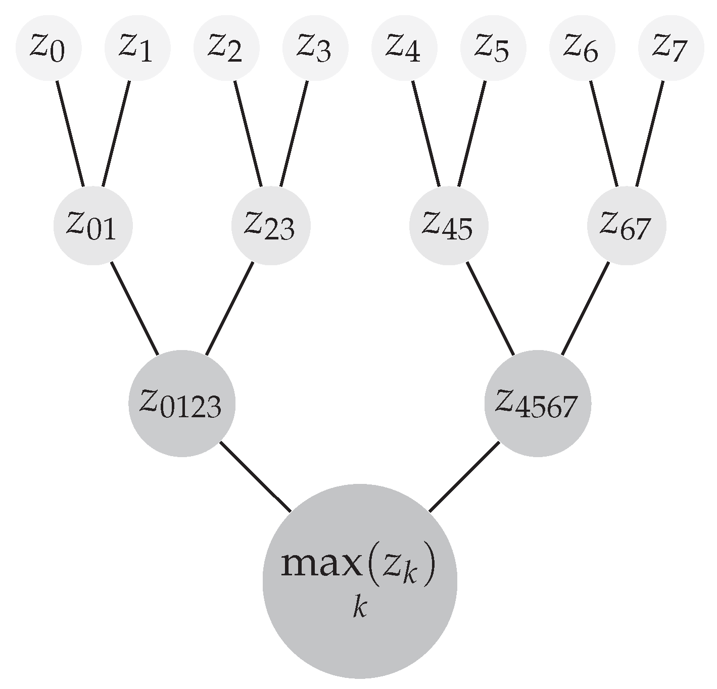
Figure 4.
Values obtained from Examples 1 and 2. (a) = 0.9946, MSE = 0.8502. (b) = 0.0449, MSE = 0.0018
Figure 4.
Values obtained from Examples 1 and 2. (a) = 0.9946, MSE = 0.8502. (b) = 0.0449, MSE = 0.0018

Figure 5.
Values obtained from imagenet image classification for 1000 classes and a custom net for MNIST digit classification for 10 classes. (a) = 0.001, MSE = 1.5205 × 10⁻⁵. (b) = 0.1111, MSE = 6.0841
Figure 5.
Values obtained from imagenet image classification for 1000 classes and a custom net for MNIST digit classification for 10 classes. (a) = 0.001, MSE = 1.5205 × 10⁻⁵. (b) = 0.1111, MSE = 6.0841
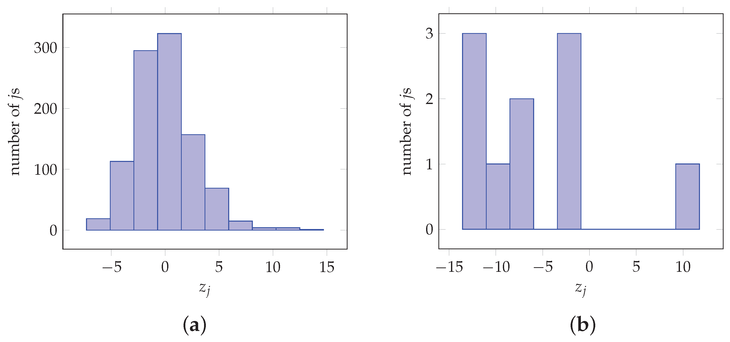
Figure 6.
Values obtained from imagenet image ResNet-50 net classification for 1000 classes. (a) Histogram of the MSE values. (b) Histogram of the values
Figure 6.
Values obtained from imagenet image ResNet-50 net classification for 1000 classes. (a) Histogram of the MSE values. (b) Histogram of the values

Figure 7.
Values obtained from imagenet image VGG-16 net classification for 1000 classes. (a) Histogram of the MSE values. (b) Histogram of the values.
Figure 7.
Values obtained from imagenet image VGG-16 net classification for 1000 classes. (a) Histogram of the MSE values. (b) Histogram of the values.

Figure 8.
Actual and proposed approximation softmax values for two inferences, namely A and B, for the VGG-16 CNN. (a) Actual softmax values for inference A. (b) Actual softmax values for inference B. (c) Proposed approximation softmax values for inference A based on architecture of Figure 2a and (18). (d) Proposed approximation softmax values for inference B based on architecture of Figure 2a and (18). (e) Proposed approximation softmax values for inference A based on architecture of Figure 2b and (30) with . (f) Proposed approximation softmax values for inference B based on architecture of Figure 2b and (30) with .
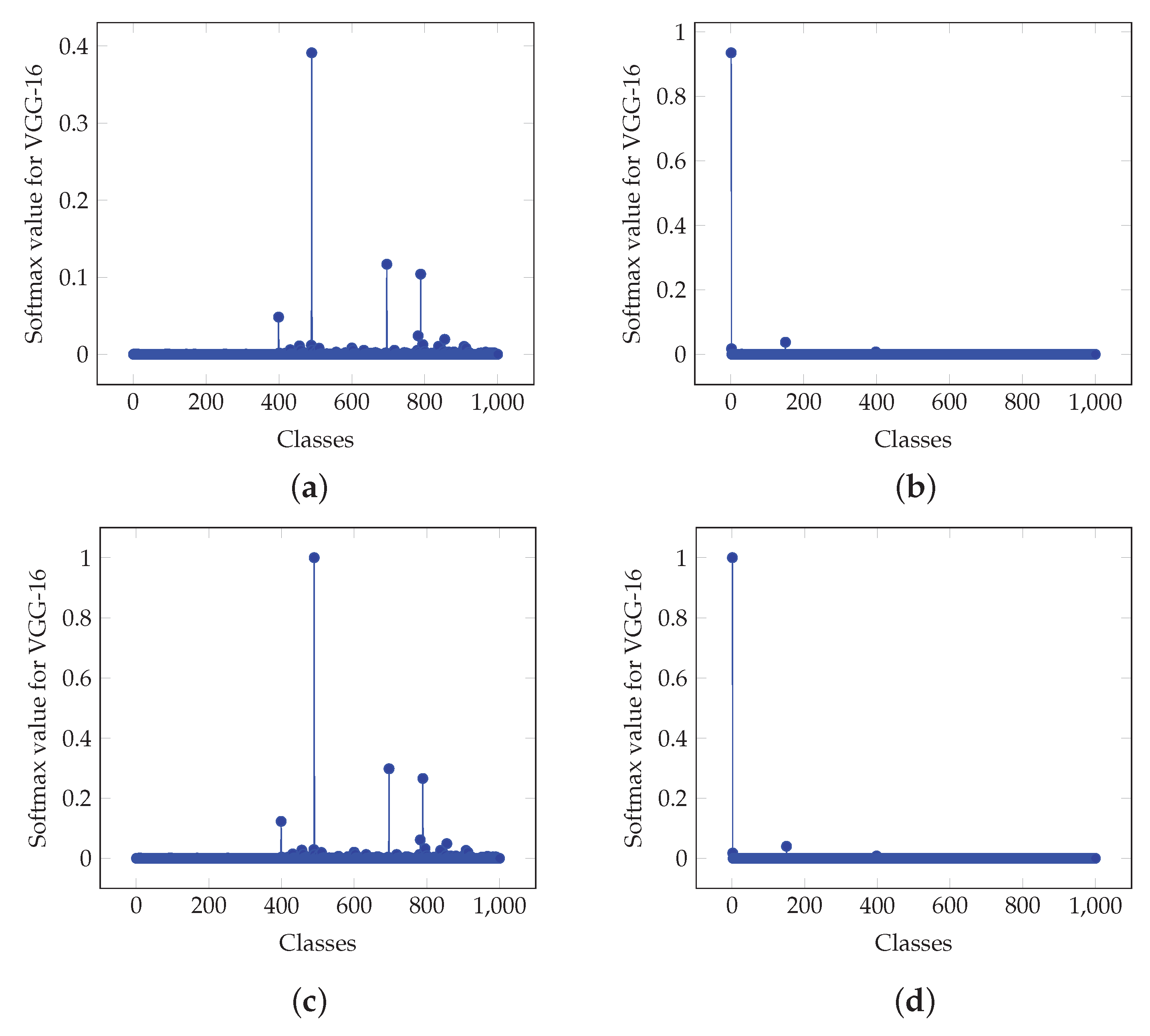

Figure 9.
Values obtained from imagenet image VGG-19 net classification for 1000 classes. (a) Histogram of the MSE values. (b) Histogram of the values.
Figure 9.
Values obtained from imagenet image VGG-19 net classification for 1000 classes. (a) Histogram of the MSE values. (b) Histogram of the values.
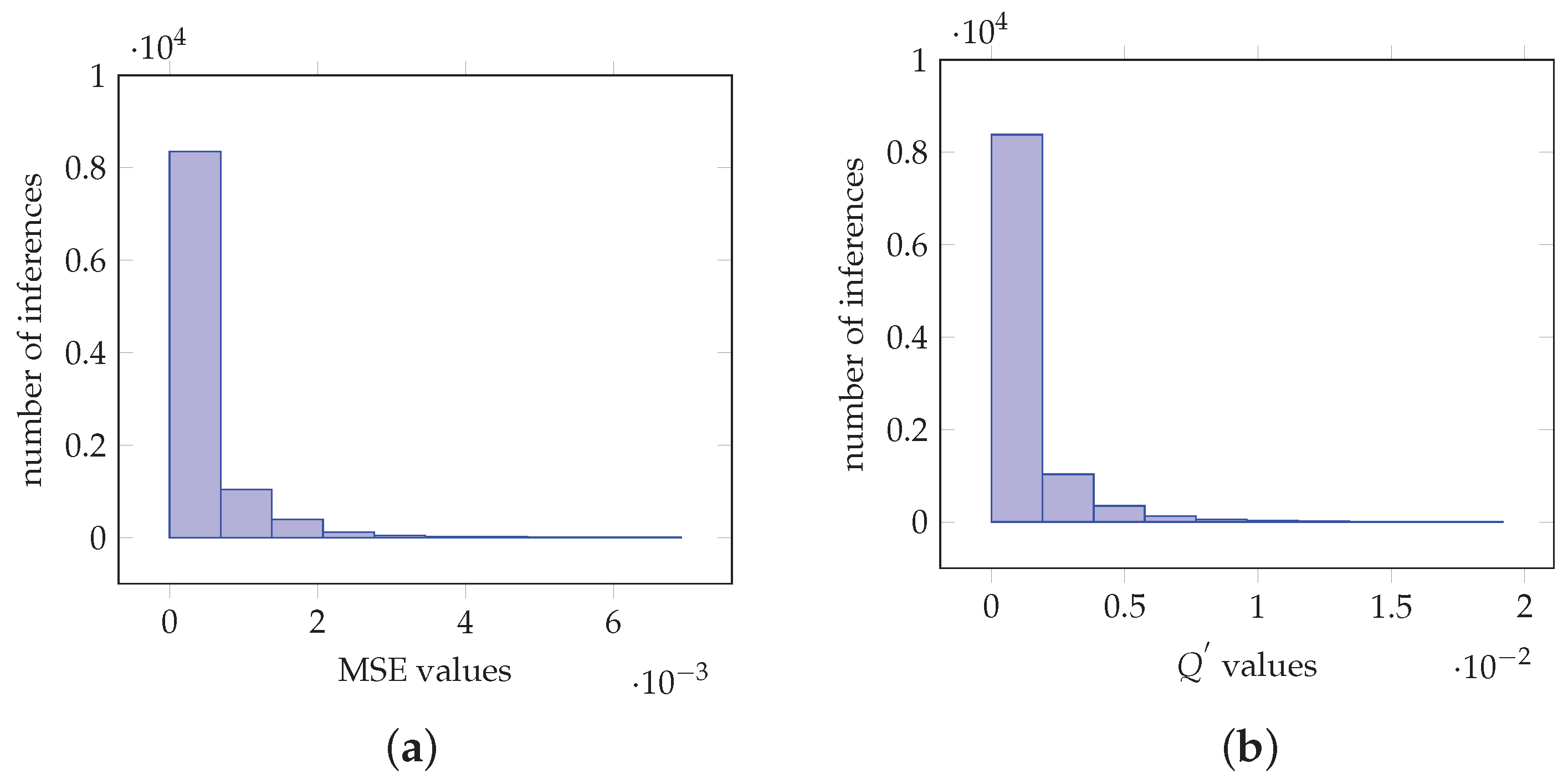
Figure 10.
Values obtained from imagenet image inceptionV3 net classification for 1000 classes. (a) Histogram of the MSE values. (b) Histogram of the values.
Figure 10.
Values obtained from imagenet image inceptionV3 net classification for 1000 classes. (a) Histogram of the MSE values. (b) Histogram of the values.
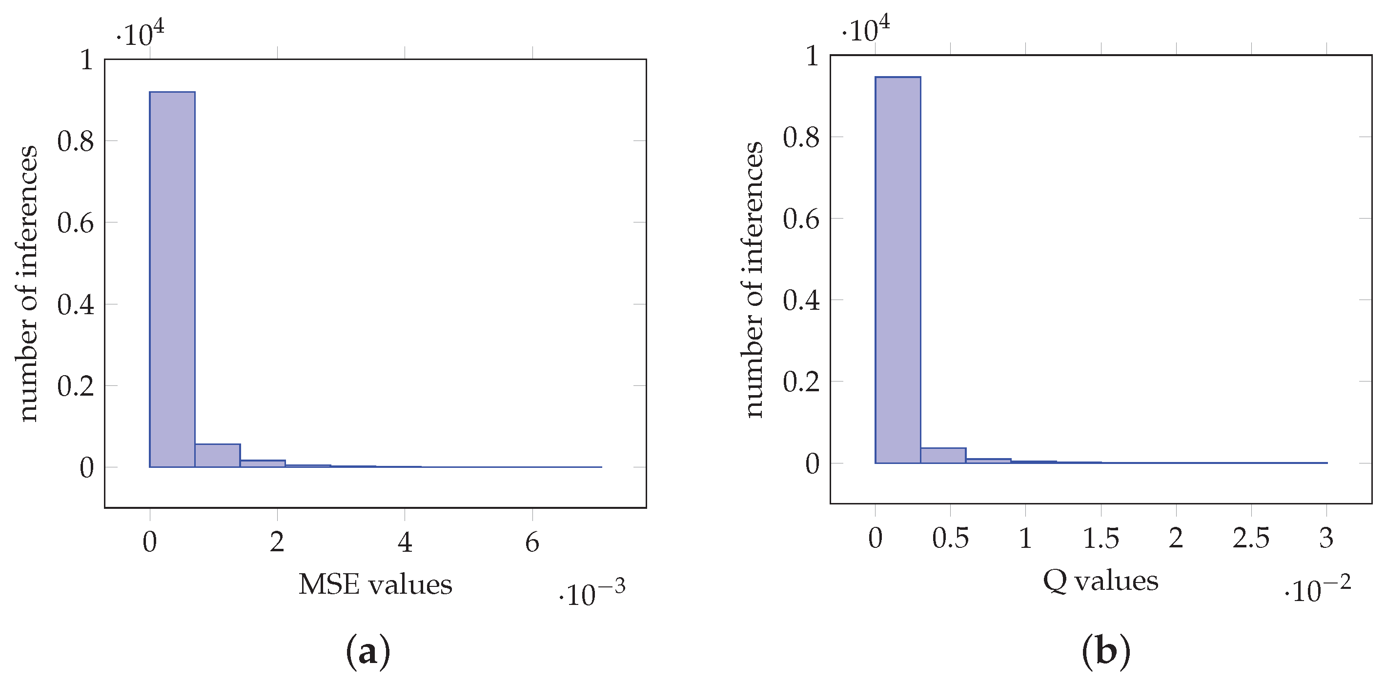
Figure 11.
Values obtained from imagenet image MobileNetV2 net classification for 1000 classes. (a) Histogram of the MSE values. (b) Histogram of the values.
Figure 11.
Values obtained from imagenet image MobileNetV2 net classification for 1000 classes. (a) Histogram of the MSE values. (b) Histogram of the values.

Figure 12.
Histograms for the MSE values for various data wordlengths for the case of 1000 inferences in the VGG-16 CNN. (a) Histograms for the MSE values for (3, 2) and (4, 2) data wordlength. (b) Histograms for the MSE values for (5, 2) and (6, 2) data wordlength.
Figure 12.
Histograms for the MSE values for various data wordlengths for the case of 1000 inferences in the VGG-16 CNN. (a) Histograms for the MSE values for (3, 2) and (4, 2) data wordlength. (b) Histograms for the MSE values for (5, 2) and (6, 2) data wordlength.

Figure 13.
Proposed architecture obtained by synthesis.
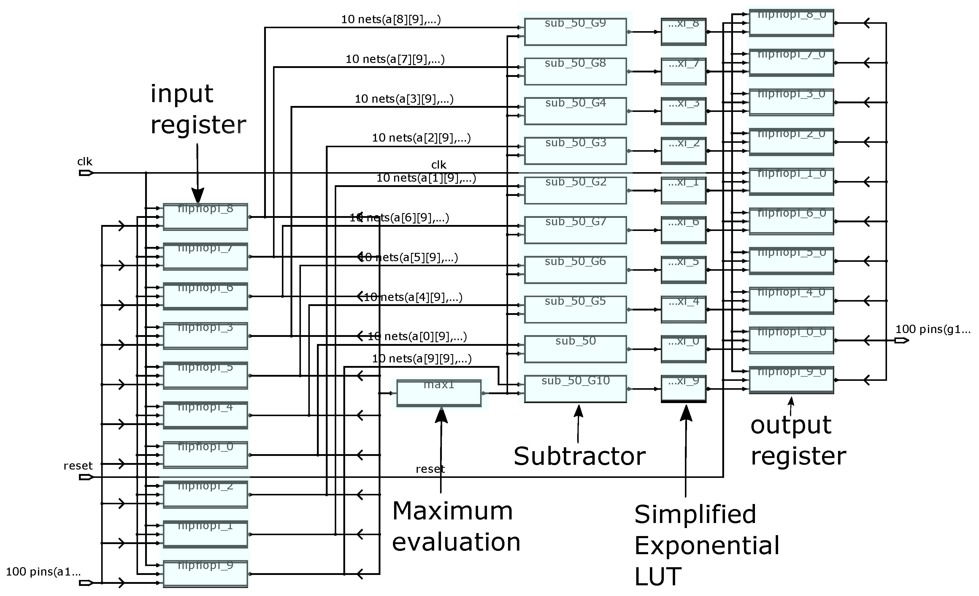
Figure 14.
Area, delay and power complexity plots for a softmax layer of size 10, for the proposed and [22] circuits in the case of -bit wordlength implemented in a standard-cell library. A, B and C in the legends denote architectures in Figure 2a, Figure 2b and [22], respectively. (a) Area vs. delay plot. (b) Power vs. delay plot.

Table 1.
Top-5 softmax values for six indicative inferences for each model. The actual softmax values and the proposed method values are obtained by (1) and (18), respectively. For the VGG-16 CNN, values obtained by (30) are also presented.

(a) ResNet-50.
| Inference | Top-5 Softmax Values | ||||
|---|---|---|---|---|---|
| (1) | |||||
| 0.75371140 | 0.027212996 | 0.018001331 | 0.014599146 | 0.014546203 | |
| 0.99992204 | 4.0420113 × 10⁻⁵ | 8.1600538 × 10⁻⁶ | 5.8431901 × 10⁻⁶ | 2.5279753 × 10⁻⁶ | |
| 0.36263093 | 0.13568024 | 0.090758167 | 0.063106202 | 0.061747193 | |
| 0.93937486 | 0.011548955 | 0.010892190 | 0.0068663955 | 0.0043140189 | |
| 0.98696542 | 0.0090351542 | 0.0010830049 | 0.00068612932 | 0.00025251327 | |
| f | 0.99833566 | 0.0015795525 | 4.6098357 × 10⁻⁵ | 2.2146454 × 10⁻⁵ | 1.0724646 × 10⁻⁵ |
| (18) | |||||
| 1 | 0.03515625 | 0.0234375 | 0.0185546875 | 0.0185546875 | |
| 1 | 0 | 0 | 0 | 0 | |
| 1 | 0.3740234375 | 0.25 | 0.173828125 | 0.169921875 | |
| 1 | 0.01171875 | 0.0107421875 | 0.0068359375 | 0.00390625 | |
| 1 | 0.0087890625 | 0.0009765625 | 0 | 0 | |
| 1 | 0.0009765625 | 0 | 0 | 0 | |
(b) VGG-16.
| Inference | Top-5 Softmax Values | ||||
|---|---|---|---|---|---|
| (1) | |||||
| 0.99999309 | 2.3484120 × 10⁻⁶ | 9.8677640 × 10⁻⁷ | 4.2830493 × 10⁻⁷ | 3.1285174 × 10⁻⁷ | |
| 0.99389344 | 0.0014656042 | 0.00072381413 | 0.00062438881 | 0.00028156079 | |
| 0.94363135 | 0.022138771 | 0.0087750498 | 0.0048798379 | 0.0047590565 | |
| 0.73901427 | 0.10941570 | 0.065981410 | 0.018329350 | 0.012467328 | |
| 0.51182884 | 0.18920843 | 0.10042682 | 0.055410255 | 0.030226296 | |
| 0.59114474 | 0.40821150 | 0.00043615574 | 0.00017272410 | 1.3683101 × 10⁻⁵ | |
| (18) | |||||
| 1 | 0 | 0 | 0 | 0 | |
| 1 | 0.0009765625 | 0 | 0 | 0 | |
| 1 | 0.0234375 | 0.0087890625 | 0.0048828125 | 0.0048828125 | |
| 1 | 0.1474609375 | 0.0888671875 | 0.0244140625 | 0.0166015625 | |
| 1 | 0.369140625 | 0.1962890625 | 0.107421875 | 0.05859375 | |
| 1 | 0.6904296875 | 0 | 0 | 0 | |
| (30) | |||||
| 0.999023438 | 0 | 0 | 0 | 0 | |
| 0.99609375 | 0.000976563 | 0 | 0 | 0 | |
| 0.954101563 | 0.021484375 | 0.008789063 | 0.004882813 | 0.00390625 | |
| 0.747070313 | 0.110351563 | 0.06640625 | 0.017578125 | 0.01171875 | |
| 0.456054688 | 0.16796875 | 0.088867188 | 0.048828125 | 0.026367188 | |
| 0.5 | 0.345703125 | 0 | 0 | 0 | |
(c) VGG-19.
| Inference | Top-5 Softmax Values | ||||
|---|---|---|---|---|---|
| (1) | |||||
| 0.99204987 | 0.0035423702 | 0.0018605839 | 0.00044701522 | 0.00035935538 | |
| 0.99999964 | 2.9884677 × 10⁻⁷ | 1.5874324 × 10⁻¹¹ | 1.5047866 × 10⁻¹¹ | 9.9192204 × 10⁻¹³ | |
| 0.99405837 | 0.0013178071 | 0.00071631809 | 0.00040839455 | 0.00027133274 | |
| 0.19257018 | 0.12952097 | 0.12107860 | 0.10589719 | 0.074582554 | |
| 0.99603385 | 0.0014963613 | 0.0010812994 | 0.00024322474 | 0.00015848021 | |
| f | 0.74559504 | 0.15503055 | 0.010651816 | 0.0081892628 | 0.0075844983 |
| (18) | |||||
| 1 | 0.0029296875 | 0.0009765625 | 0 | 0 | |
| 1 | 0 | 0 | 0 | 0 | |
| 1 | 0.0009765625 | 0 | 0 | 0 | |
| 1 | 0.671875 | 0.6279296875 | 0.548828125 | 0.38671875 | |
| 1 | 0.0009765625 | 0.0009765625 | 0 | 0 | |
| 1 | 0.20703125 | 0.013671875 | 0.0107421875 | 0.009765625 | |
(d) InceptionV3.
| Inference | Top-5 Softmax Values | ||||
|---|---|---|---|---|---|
| (1) | |||||
| 0.98136926 | 0.00067191740 | 0.00022632803 | 0.00020886297 | 0.00018680355 | |
| 0.52392030 | 0.17270486 | 0.12838276 | 0.0024479097 | 0.0017230138 | |
| 0.61721277 | 0.042022489 | 0.038270507 | 0.011870607 | 0.0036431390 | |
| 0.96187764 | 0.0011140818 | 0.00084153039 | 0.00069097377 | 0.00045776321 | |
| 0.99643219 | 0.00058087677 | 0.00015713122 | 5.3965716 × 10⁻⁵ | 4.0285959 × 10⁻⁵ | |
| f | 0.45723280 | 0.41415739 | 0.00078048115 | 0.00071852183 | 0.00068869896 |
| (18) | |||||
| 1 | 0 | 0 | 0 | 0 | |
| 1 | 0.3291015625 | 0.244140625 | 0.00390625 | 0.0029296875 | |
| 1 | 0.0673828125 | 0.0615234375 | 0.0185546875 | 0.005859375 | |
| 1 | 0.0009765625 | 0 | 0 | 0 | |
| 1 | 0 | 0 | 0 | 0 | |
| 1 | 0.9052734375 | 0.0009765625 | 0.0009765625 | 0.0009765625 | |
(e) MobileNetV2.
| Inference | Top-5 Softmax Values | ||||
|---|---|---|---|---|---|
| (1) | |||||
| 0.81305408 | 0.014405688 | 0.012406061 | 0.0091119893 | 0.0077789603 | |
| 0.95702046 | 0.0042284634 | 0.0040278519 | 0.0020813416 | 0.00098748843 | |
| 0.49231452 | 0.022776684 | 0.020905942 | 0.018753875 | 0.018386556 | |
| 0.60401917 | 0.29827181 | 0.015593613 | 0.010511264 | 0.0038427035 | |
| 0.97501647 | 0.0032496843 | 0.0014790110 | 0.0008857667 | 0.00076536590 | |
| f | 0.87092900 | 0.022609057 | 0.0044059716 | 0.0023696721 | 0.0014177967 |
| (18) | |||||
| 1 | 0.017578125 | 0.0146484375 | 0.0107421875 | 0.0087890625 | |
| 1 | 0.00390625 | 0.00390625 | 0.001953125 | 0.0009765625 | |
| 1 | 0.0458984375 | 0.0419921875 | 0.0380859375 | 0.037109375 | |
| 1 | 0.4931640625 | 0.025390625 | 0.0166015625 | 0.005859375 | |
| 1 | 0.0029296875 | 0.0009765625 | 0 | 0 | |
| 1 | 0.025390625 | 0.0048828125 | 0.001953125 | 0.0009765625 | |
Table 2.
Area, delay and power consumption for the 10-class softmax layer output of a convolutional neural network (CNN).
(a) Architecture of Figure 2a.
(a) Architecture of Figure 2a.
| Delay (ns) | Area (m) | Power (w) |
|---|---|---|
| 2.93 | 16,891 | 1611.6 |
| 3.43 | 17,293 | 1423.7 |
| 3.95 | 15,550 | 1070.5 |
| 4.42 | 15,788 | 936.8 |
| 4.94 | 15,084 | 812.4 |
| 5.47 | 15,349 | 503.5 |
(b) Architecture in [22].
(b) Architecture in [22].
| Delay (ns) | Area (m) | Power (w) |
|---|---|---|
| 3.99 | 43,576 | 3228.2 |
| 5.19 | 32,968 | 1695.1 |
| 6.45 | 25,445 | 871.8 |
| 7.95 | 26,358 | 714.4 |
| 9.44 | 25,846 | 624.9 |
| 10.41 | 26,154 | 570.2 |
(c) Architecture of Figure 2b with p = 5.
(c) Architecture of Figure 2b with p = 5.
| Delay (ns) | Area (m) | Power (w) |
|---|---|---|
| 3.42 | 27,615 | 1933.2 |
| 3.92 | 25,597 | 1576.3 |
| 4.91 | 23,654 | 1216.4 |
| 5.42 | 21,458 | 1050.6 |
| 6.45 | 20,251 | 838.6 |
| 7.94 | 20,147 | 636.1 |
© 2020 by the authors. Licensee MDPI, Basel, Switzerland. This article is an open access article distributed under the terms and conditions of the Creative Commons Attribution (CC BY) license (http://creativecommons.org/licenses/by/4.0/).
Share and Cite
MDPI and ACS Style
Kouretas, I.; Paliouras, V. Hardware Implementation of a Softmax-Like Function for Deep Learning. Technologies 2020, 8, 46. https://0-doi-org.brum.beds.ac.uk/10.3390/technologies8030046
AMA Style
Kouretas I, Paliouras V. Hardware Implementation of a Softmax-Like Function for Deep Learning. Technologies. 2020; 8(3):46. https://0-doi-org.brum.beds.ac.uk/10.3390/technologies8030046
Chicago/Turabian StyleKouretas, Ioannis, and Vassilis Paliouras. 2020. "Hardware Implementation of a Softmax-Like Function for Deep Learning" Technologies 8, no. 3: 46. https://0-doi-org.brum.beds.ac.uk/10.3390/technologies8030046
Note that from the first issue of 2016, this journal uses article numbers instead of page numbers. See further details here.