Modelling Trade Durations Using Dynamic Logarithmic Component ACD Model with Extended Generalised Inverse Gaussian Distribution

Abstract

This paper proposes a logarithmic version of the two-component ACD (LogCACD) model with no restrictions on the sign of the model parameters while allowing the expected durations to be decomposed into the long- and short-run components to capture the dynamics of these durations. The extended generalised inverse Gaussian (EGIG) distribution is used for the error distribution as its hazard function consists of a roller-coaster shape for certain parameters’ values. An empirical application from the trade durations of International Business Machines stock index has been carried out to investigate this proposed model. Extensive comparisons are carried out to evaluate the modelling and forecasting performances of the proposed model with several benchmark models and different specifications of error distributions. The result reveals that the LogCACD_EGIG(1,1) model gives the best in-sample fit based on the Akaike information criterion and other criteria. Furthermore, the estimated parameters obtained through the maximum likelihood estimation confirm the existence of the roller-coaster-shaped hazard function. The examination of LogCACD_EGIG(1,1) model also provides the best out-of-sample forecasts evaluated based on the mean square forecast error using the Hansen’s model confidence set. Lastly, different levels of time-at-risk forecasts are provided and tested with Kupiec likelihood ratio test.

1. Introduction

In finance, duration is defined as the time interval between two consecutive events. For example, duration data that have been studied by researchers are trade, quote, price, transaction, and volume. As discussed by [1], financial durations played an important role in understanding and processing of private and public information in a financial market. With the advancement of technology, high frequency financial duration data can be recorded and are collected in irregular time intervals. In general, they show a strong autocorrelation which can be used to study the intraday market behaviours and dynamic of trades.

The duration models originated from the family of autoregressive conditional duration (ACD) model introduced by [2] and treated the transaction arrival time as a random variable in the dependent point process where its conditional intensity depends on the past duration. In the early stage, ACD models have been expressed in a linear model specification consisting of non-negative model parameters and non-negative error distributions such as the exponential (Exp) and Weibull (Wei) distributions [2] and the generalised gamma (GG) distribution [3]. The limitation of these models is whenever some other variables having negative coefficients are assigned to the linear autoregressive equation, the durations might become negative. Meanwhile, it is quite frequent that these ACD models will impose an exponential decay pattern on the autocorrelation function and, in general, will not account for the long-range dependence in durations. Therefore, the logarithmic ACD (LogACD) model of [4] was introduced with no restrictions on the sign of the parameters to guarantee the positiveness of the process and the fractionally integrated ACD (FIACD) model of [5] was introduced to capture the long-range dependence in durations, which is shown to be more flexible than the linear ACD model. Recently, several nonlinear ACD models have been developed to better delineate the trade duration process, see for example the threshold ACD model [6], the asymmetric ACD and asymmetric LogACD models [7], and the augmented ACD model [8]. An informative review on the various ACD models with its applications can be obtained in [9,10,11].

It being the case that most of the ACD models belong to the family of one-component models, [12] introduced the two-component ACD (CACD) model to fit the International Business Machines (IBM) trade durations to measure the impact of durations on the price volatility. The main feature of this duration model is that it consists of a long-run (trend) component and a short-run (transitory) component, and the sum of these two components establishes a long-range dependence in the duration process, which helps in capturing the complexity of duration dynamics in contrast to the one-component ACD models. To this end, [13] developed an alternative way of capturing long-range dependence in the trade duration series by extending the component multiplicative error model. However, little is known about the extension of the CACD model with no restrictions on the sign of the parameters, and hence we are keen to answer the research question of whether the extended CACD model with no sign restrictions will provide a better fit to the data as compared to the one-component models as well as the CACD model.

The choice of error distributions plays an important role in ACD modelling. [2] introduced the basic ACD model by considering the Exp and Wei as the error distributions. The Exp distribution with a constant hazard function and the Wei distribution with monotonically increasing or decreasing hazard function, however, are too restrictive, and thus, various error distributions have been considered to provide greater flexibility to the constructed models. Some examples include the GG distribution [3], the Burr type XII (Burr) distribution [14], the generalised F distribution [15], the Pareto distribution [16], the Lognormal distribution [17], the extended Weibull distribution [18], the Fréchet distribution [19], the generalised beta of type 2 (GB2) distribution [20] and the mixture of GB2 distribution [21]. Comparison of the ACD modelling performance using various distributions was addressed by [22,23,24], providing distributions either monotonically increasing, decreasing or non-monotonic shapes such as bathtub or upside-down-bathtub shape of the hazard function constituting of, at most, a single turning point. To the best of our knowledge, there has thus far been relatively little research into this area where most of the ACD models with error distributions have only a single turning point hazard function. In this aspect, we are interested to study this to see if the hazard function of the error distribution consisting of more than one turning point with a roller-coaster shape would help to increase the flexibility of the model.

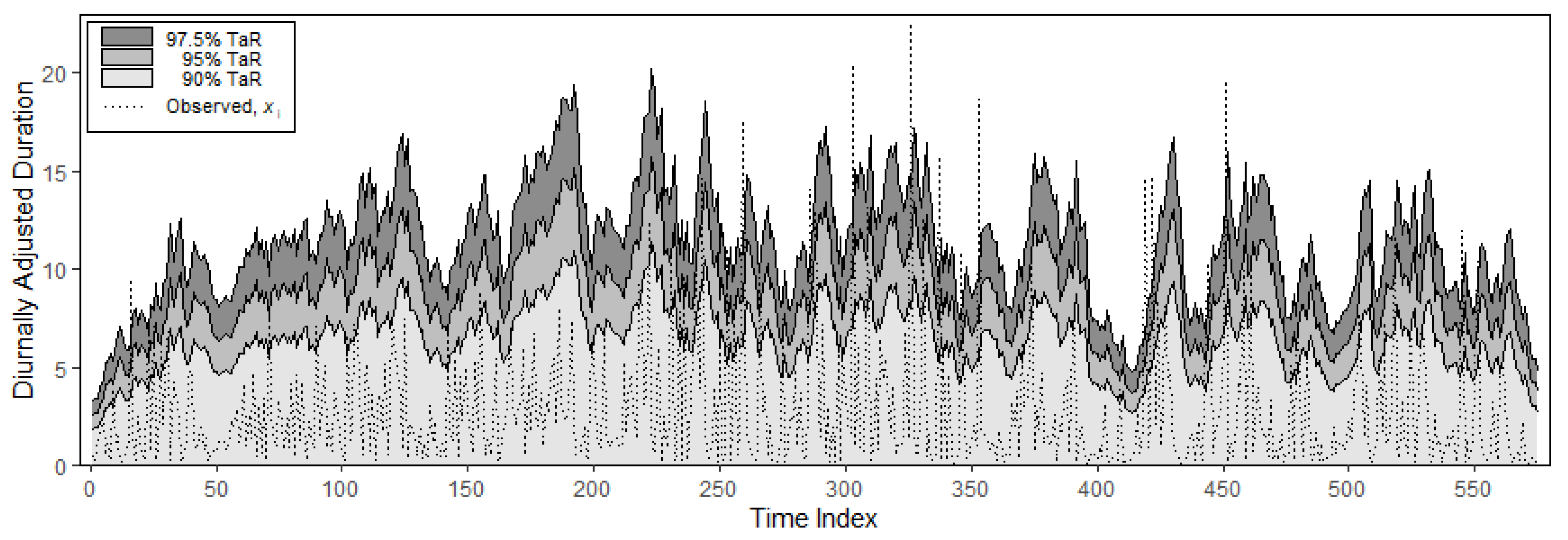
The liquidity risk such as the minimal time without any trade occurring is valuable for market makers and traders and is analogous to the value-at-risk introduced in volatility literature. Time-at-risk (TaR) is defined as the extreme risk of time between two consecutive transactions at a certain risk level. [25] showed that the TaR can be calculated from the product of the conditional expectation of durations and the inverse of the cumulative distribution associated with the error term. In the meantime, [21] used the basic ACD models with mixed distribution to compute the TaR and conditional TaR (CTaR) forecasts of trade durations, and the TaR performance was then evaluated using violation rate and quantile loss function. The performances of TaR and CTaR were further tested by employing some other common backtests as illustrated by [26,27] to confirm the accuracy of their forecasts.

The contribution of this paper is threefold. Firstly, we propose the logarithmic CACD (LogCACD) model, which allows for no restrictions on the sign of the parameters while the conditional expectation of durations is decomposed into the long- and short-run components. As the error distribution is a crucial factor in constructing a model, our second aim is to model the duration data using the LogCACD model with flexible extended generalised inverse Gaussian (EGIG) distribution having the roller-coaster-shaped hazard function. The effects of model specification and error distribution on the performances of various ACD models are then examined by comparing the in-sample model fits and out-of-sample forecasts. Subsequently, the in-sample model fitting performance is evaluated using several criteria and loss functions while the out-of-sample forecasts are tested using the model confidence set (MCS) procedure of [28] to acquire a superior set of models (SSM). Lastly, the empirical study of IBM trade durations is investigated with the detailed illustration of the model fitting and forecasts of TaR under various risk levels. It follows that the SSM are computed and the accuracy of the TaR forecasts is tested by the Kupiec likelihood ratio (KLR) test [26].

The remainder of this paper is organised as follows. Section 2 reviews several existing ACD models including the CACD model and the motivation of the LogCACD model, while Section 3 introduces the EGIG distribution and other error distributions adopted for these duration models. Section 4 describes the empirical data used in the preliminary analysis, and Section 5 reports the model fitting and forecasting results as well as the forecast of TaR. Finally, Section 6 concludes the paper.

2. The General Class of ACD Models

Let $x_i^{\ast }$ be the $i$-th duration between two consecutive transactions occurring at random times $t_i$ and $t_{i-1}$ such that

$$x_i^{\ast }=t_i-t_{i-1}, i=1,2,\dots ,N,$$

and a sequence of diurnally adjusted durations, $x_i$ is calculated by

$$x_i=\frac{x_i^{\ast }}{\mathsf{\Phi }\left(t_i\right)},$$

(1)

where $\mathsf{\Phi }\left(t_i\right)$ is the deterministic function used to remove the diurnal effect of $x_i^{\ast }$ (see [29]).

2.1. Basic ACD and CACD Models

Let ${\psi }_i$ be the conditional expectation of $x_i$ which is defined as

$${\psi }_i=\mathrm{E}\left(x_i|x_{i-1},x_{i-2},\dots ,x_1\right)=\mathrm{E}\left(x_i|F_{i-1}\right),$$

where $F_{i-1}=\left\{x_{i-1},x_{i-2},\dots ,x_1\right\}$ is the information set available up to $t_{i-1}$. Then, the diurnally adjusted duration $x_i$ at time $t_i$ can be modelled as

$$x_i={\psi }_i{\epsilon }_i,$$

(2)

where ${\epsilon }_i$ is a sequence of independent and identically distributed non-negative random variables with a known probability density function (pdf) $f(·)$ such that $\mathrm{E}\left({\epsilon }_i\right)=1$ and ${\epsilon }_i$ is independent of $F_{i-1}$.

(a)

Basic ACD model

The basic ACD ($𝒫$,$𝒬$) model specification of orders $𝒫$ and $\mathcal{Q}$ is given by

$${\psi }_i=\vartheta +{{\displaystyle \sum }}_{j=1}^{𝒫}{\alpha }_j{x}_{i-j}+{{\displaystyle \sum }}_{k=1}^{𝒬}{\beta }_k{\psi }_{i-k}$$

(3)

where the parameters $\vartheta >0$, ${\alpha }_j\ge 0$ and ${\beta }_k\ge 0$ are restricted to be non-negative to ensure the positivity of ${\psi }_i.$ The unconditional expectation of $x_i$ can be calculated from

$$\mu =\mathrm{E}\left(x_i\right)=\frac{\vartheta }{1-{{\displaystyle \sum }}_{j=1}^{𝒫}{\alpha }_j-{{\displaystyle \sum }}_{k=1}^{𝒫}{\beta }_k}$$

(4)

if ${{\displaystyle \sum }}_{j=1}^{𝒫}{\alpha }_j+{{\displaystyle \sum }}_{k=1}^{𝒫}{\beta }_k<1$

(b)

CACD model

Using the Equations (3) and (4), a dynamic structure of ${\psi }_i$ under the basic ACD(1,1) model can be written as

$$\begin{gathered} {\psi }_i=\mu \left(1-{\alpha }_1-{\beta }_1\right)+{\alpha }_1{x}_{i-1}+{\beta }_1{\psi }_{i-1} \\ =\mu +{\alpha }_1\left(x_{i-1}-\mu \right)+{\beta }_1\left({\psi }_{i-1}-\mu \right), \end{gathered}$$

(5)

where$\mu$ is the constant trend of ${\psi }_i$ and $\left(x_{i-1}-\mu \right)$ is the shock of duration.

For a more general specification, the constant trend $\mu$ can be modelled in a dynamic structure (denoted as ${\psi }_{i,1}$), which will be allowed to evolve slowly in an autoregressive manner. More specifically, the dynamic trend of the conditional expectation of $x_i$, ${\psi }_{i,1}$ can be defined as

$${\psi }_{i,1}={\omega }_{\mu }+{\rho }_{\mu }{\psi }_{i-1,1}+{\alpha }_{\mu }\left(x_{i-1}-{\psi }_{i-1}\right),$$

(6)

which is called the long-run component. On the other hand, a short-run component, ${\psi }_{i,2}$, is defined as the difference between ${\psi }_i$ and the long-run component, ${\psi }_{i,1}$. To be more specific, the short-run component, ${\psi }_{i,2}$, is

$${\psi }_{i,2}={\psi }_i-{\psi }_{i,1}={\alpha }_1\left(x_{i-1}-{\psi }_{i-1,1}\right)+{\beta }_1\left({\psi }_{i-1}-{\psi }_{i-1,1}\right).$$

(7)

Hence, the CACD(1,1) model specification can be written as

$${\psi }_i={\psi }_{i,1}+{\psi }_{i,2},$$

(8)

$${\psi }_{i,1}={\omega }_{\mu }+{\rho }_{\mu }{\psi }_{i-1,1}+{\alpha }_{\mu }\left(x_{i-1}-{\psi }_{i-1}\right),$$

and

$${\psi }_{i,2}=\left({\alpha }_1+{\beta }_1\right){\psi }_{i-1,2}+{\alpha }_1\left(x_{i-1}-{\psi }_{i-1}\right).$$

Note that the duration innovation $\left(x_{i-1}-{\psi }_{i-1}\right)$ will drive both the long- and short-run components at the rate of ${\alpha }_{\mu }$ and ${\alpha }_1$, respectively. The long- and short-run components have the respective unconditional mean of $\mathrm{E}\left({\psi }_{i,1}\right)={\omega }_{\mu }/\left(1-{\rho }_{\mu }\right)$ and $\mathrm{E}\left({\psi }_{i,2}\right)=0$ which leads to the long-run component converging into a constant level at ${\omega }_{\mu }/\left(1-{\rho }_{\mu }\right)$ and the short-run component mean-reverting to zero at a geometric rate of $\left({\alpha }_1+{\beta }_1\right)$ when $0<\left({\alpha }_1+{\beta }_1\right)<1.$ If $0<\left({\alpha }_1+{\beta }_1\right)<{\rho }_{\mu }<1$, then the long-run component has much slower mean-reverting rate or more persistent than the short-run component. For CACD(1,1) model, the following non-negativity constraints are needed to ensure the positivity of the conditional expectation of durations:

$${\omega }_{\mu }>0, {\rho }_{\mu }>0,{\alpha }_{\mu }>0,{\alpha }_1>0, {\beta }_1>0\mathrm{and}0<{\alpha }_{\mu }<{\alpha }_1,$$

which are compatible with the stationarity conditions of $\left({\alpha }_1+{\beta }_1\right)<1$ and ${\rho }_{\mu }<1$. Principally, the CACD model resembles the component generalised autoregressive conditional heteroskedasticity (CGARCH) model, hence the constraints’ development of the CACD(1,1) model is in analogous to the CGARCH(1,1) model and the details of the illustrations can be found in the appendix of [30].

Essentially, the conditional expectation of diurnally adjusted duration for the CACD(1,1) model in Equation (8) can be written as the basic ACD(2,2) model as follows:

$$\begin{gathered} {\psi }_i=\left(1-{\alpha }_1-{\beta }_1\right){\omega }_{\mu }+\left({\alpha }_{\mu }+{\alpha }_1\right)x_{i-1}+\left[-{\alpha }_{\mu }\left({\alpha }_1+{\beta }_1\right)-{\alpha }_1{\rho }_{\mu }\right]x_{i-2} \\ +\left({\rho }_{\mu }+{\beta }_1-{\alpha }_{\mu }\right){\psi }_{i-1}+\left[{\alpha }_{\mu }\left({\alpha }_1+{\beta }_1\right)-{\beta }_1{\rho }_{\mu }\right]{\psi }_{i-2}. \end{gathered}$$

The above can be reduced to the basic ACD(1,1) model by setting ${\alpha }_1={\beta }_1=0$ and ${\rho }_{\mu }={\alpha }_{\mu }+{\beta }_{\mu }$. This indicates that the CACD(1,1) model encompasses higher order of the basic ACD model as discussed by [12].

2.2. LogACD and LogCACD Models

To ensure the positiveness of the conditional expectation of durations with no restrictions on the sign of the parameters of the ACD model specification, [4] defined ${\psi }_i$ as the logarithmic of the conditional expectation of $x_i$, so that:

$${\psi }_i=\ln \left[\mathrm{E}\left(x_i|x_{i-1},x_{i-2},\dots ,x_1\right)\right]=\ln \left[\mathrm{E}\left(x_i|F_{i-1}\right)\right].$$

Consequently, the diurnally adjusted duration, $x_i$, can be modelled as

$$x_i=e^{{\psi }_i}{\epsilon }_i.$$

(9)

(a)

LogACD model

The LogACD($𝒫$,$𝒬$) model specification of orders $𝒫$ and $\mathcal{𝒬}$ is given by

$${\psi }_i=\vartheta +{{\displaystyle \sum }}_{j=1}^{𝒫}{\alpha }_j\mathrm{l}\mathrm{n}\left(x_{i-j}\right)+{{\displaystyle \sum }}_{k=1}^{𝒬}{\beta }_k{\psi }_{i-k}$$

(10)

where ${\alpha }_j$ and ${\beta }_k$ are parameters without positivity constraints. For the process to be weakly stationary, the constraint $|{{\displaystyle \sum }}_{j=1}^{𝒫}{\alpha }_j+{{\displaystyle \sum }}_{k=1}^{𝒫}{\beta }_k|<1$ is required.

(b)

LogCACD(1,1) model

Motivated by the flexibility of CACD(1,1) model specification and imposing no restrictions on the sign of the parameters of LogACD model, we propose the logarithmic version of the CACD(1,1) called LogCACD(1,1) model, which shares the similar structure with the CACD(1,1) model defined as

$${\psi }_i={\psi }_{i,1}+{\psi }_{i,2},$$

(11)

$${\psi }_{i,1}={\omega }_{\mu }+{\rho }_{\mu }{\psi }_{i-1,1}+{\alpha }_{\mu }\left[\ln \left(x_{i-1}\right)-{\psi }_{i-1}\right],$$

and

$${\psi }_{i,2}=\left({\alpha }_1+{\beta }_1\right){\psi }_{i-1,2}+{\alpha }_1\left[\ln (x_{i-1})-{\psi }_{i-1}\right],$$

where ${\psi }_{i,1}$ and ${\psi }_{i,2}$ are, respectively, the long- and short-run components. With no restrictions on the sign of the parameters, LogCACD model requires fewer restrictions on the model parameters as compared with CACD model. To avoid interchangeable between the two components, we impose the restriction $\left|{\alpha }_1+{\beta }_1\right|<\left|{\rho }_{\mu }\right|<1$, which is also the stationarity condition of $\ln (x_i)$.

Analogous to the CACD(1,1) model, the logarithmic of the conditional expectation of diurnally adjusted duration for LogCACD(1,1) model in Equation (11) can be rewritten as the LogACD(2,2) stated as

$$\begin{gathered} {\psi }_i=\left(1-{\alpha }_1-{\beta }_1\right){\omega }_{\mu }+\left({\alpha }_{\mu }+{\alpha }_1\right)\ln (x_{i-1})+\left[-{\alpha }_{\mu }\left({\alpha }_1+{\beta }_1\right)-{\alpha }_1{\rho }_{\mu }\right]\ln (x_{i-2}) \\ +\left({\rho }_{\mu }+{\beta }_1-{\alpha }_{\mu }\right){\psi }_{i-1}+\left[{\alpha }_{\mu }\left({\alpha }_1+{\beta }_1\right)-{\beta }_1{\rho }_{\mu }\right]{\psi }_{i-2}. \end{gathered}$$

It can be reduced to the LogACD(1,1) model by assigning ${\alpha }_1={\beta }_1=0$ and ${\rho }_{\mu }={\alpha }_{\mu }+{\beta }_{\mu }$.

3. Error Distributions for ACD Models and Estimation

To improve the flexibility of hazard function in ACD models, we use the EGIG distribution proposed by [31], which contains more than one turning point in the hazard function. Further details of the EGIG distribution, its statistical properties, inferences and applications are available in [32,33,34]. To facilitate the comparison, several error distributions such as Wei, GG, Burr and GB2 are also considered.

Let $y_i$ be a EGIG distributed random variable, such that $y_i~\mathrm{EGIG}\left(\lambda ,\delta ,v,w\right)$. The pdf, cumulative density function (cdf) and hazard function of $y_i$, are, respectively, given by

$$f\left(y_i\right)=\frac{\delta y_i^{\lambda -1}}{2v^{\lambda /\delta } K_{\lambda /\delta }\left(w\right)}\exp \left[-\frac{w}{2}\left(v^{-1}{y}_i^{\delta }+v{y}_i^{-\delta }\right)\right],y_i>0,$$

(12)

$$F\left(y_i\right)=\frac{\gamma \left(\frac{\lambda }{\delta } , \frac{w{y}_i^{\delta }}{2v}, \frac{w^2}{4}\right)}{2^{1-\lambda /\delta } \left(w^{\lambda /\delta }\right) K_{\lambda /\delta }\left(w\right)},$$

(13)

and

$$h\left(y_i\right)=\frac{\delta y_i^{\lambda -1}}{v^{ \lambda /\delta }\left[2K_{\lambda /\delta }\left(w\right)-2^{\lambda /\delta } w^{-\lambda /\delta } \gamma \left(\frac{\lambda }{\delta } , \frac{w{y}_i^{\delta }}{2v}, \frac{w^2}{4}\right)\right]}\exp \left[-\frac{w}{2}\left(v^{-1}{y}_i^{\delta }+v{y}_i^{-\delta }\right)\right],$$

(14)

where$\lambda \in ℝ$, $\delta >0$, $w>0$, $v>0$, $K_{\lambda /\delta }\left(w\right)$ is the modified Bessel function of the third kind with index $\frac{\lambda }{\delta }$ and $\gamma \left(\frac{\lambda }{\delta }, \frac{w{y}_i^{\delta }}{2v}, \frac{w^2}{4}\right)$ is the generalised incomplete gamma function, which can be defined as the power series expansion in its general form of $\exp \left(-c{t}^{-1}\right)$ given by

$$\gamma \left(\eta ,z,c\right)={{\displaystyle \int }}_0^z{t}^{\eta -1}\exp \left(-t-c{t}^{-1}\right)dt={{\displaystyle \sum }}_{k=0}^{\infty }\frac{{\left(-c\right)}^k}{k!}\gamma \left(\eta -k,z\right),$$

with $\gamma \left(\eta -k,z\right)={{\displaystyle \int }}_0^z{t}^{\eta -k-1}\exp \left(-t\right)dt$ is the ordinary incomplete gamma function.

Let ${\epsilon }_i$ be a standardised EGIG distributed random variable such that

$$\mathrm{E}\left({\epsilon }_i\right)=\frac{v^{1/\delta }{K}_{\left(\lambda +1\right)/\delta }\left(w\right)}{K_{\lambda /\delta }\left(w\right)}=1.$$

Then, the scale parameter $v$ can be reparametrised as

$$v={\left[\frac{K_{\lambda /\delta }\left(w\right)}{K_{\left(\lambda +1\right)/\delta }\left(w\right)}\right]}^{\delta }.$$

By substituting the $v$ into Equations (12)–(14), the corresponding pdf, cdf and hazard function of ${\epsilon }_i~\mathrm{EGIG}\left(\lambda ,\delta ,{\left[\frac{K_{\lambda /\delta }\left(w\right)}{K_{\left(\lambda +1\right)/\delta }\left(w\right)}\right]}^{\delta },w\right)$are expressed as

$$f\left({\epsilon }_i\right)=\frac{\delta {\epsilon }_i^{\lambda -1}{\left[K_{\left(\lambda +1\right)/\delta }\left(w\right)\right]}^{\lambda }}{2{\left[K_{\lambda /\delta }\left(w\right)\right]}^{\lambda +1}}\exp \left\{-\frac{w}{2}\left[{\left(\frac{{\epsilon }_i K_{\left(\lambda +1\right)/\delta }\left(w\right)}{K_{\lambda /\delta }\left(w\right)}\right)}^{\delta }+{\left(\frac{{\epsilon }_i K_{\left(\lambda +1\right)/\delta }\left(w\right)}{K_{\lambda /\delta }\left(w\right)}\right)}^{-\delta }\right]\right\},$$

(15)

$$F\left({\epsilon }_i\right)=\frac{\gamma \left(\frac{\lambda }{\delta } , \frac{w }{2}{\left[\frac{{\epsilon }_i K_{\left(\lambda +1\right)/\delta }\left(w\right)}{K_{\lambda /\delta }\left(w\right)}\right]}^{\delta }, \frac{w^2}{4}\right)}{2^{1-\lambda /\delta } w^{\lambda /\delta } K_{\lambda /\delta }\left(w\right)},$$

(16)

and

$$h\left({\epsilon }_i\right)=\frac{\delta {\epsilon }_i^{\lambda -1}{\left(K_{\left(\lambda +1\right)/\delta }\left(w\right)\right)}^{\mathsf{\lambda }}\exp \left\{-\frac{w}{2}\left[{\left(\frac{{\epsilon }_i K_{\left(\lambda +1\right)/\delta }\left(w\right)}{K_{\lambda /\delta }\left(w\right)}\right)}^{\delta }+{\left(\frac{{\epsilon }_i K_{\left(\lambda +1\right)/\delta }\left(w\right)}{K_{\lambda /\delta }\left(w\right)}\right)}^{-\delta }\right]\right\}}{{\left(K_{\lambda /\delta }\left(w\right)\right)}^{\mathsf{\lambda }}\left[2K_{\lambda /\delta }\left(w\right)-2^{\lambda /\delta } w^{-\lambda /\delta } \gamma \left(\frac{\lambda }{\delta }, \frac{w }{2}{\left[\frac{{\epsilon }_i K_{\left(\lambda +1\right)/\delta }\left(w\right)}{K_{\lambda /\delta }\left(w\right)}\right]}^{\delta }, \frac{w^2}{4}\right)\right]}.$$

(17)

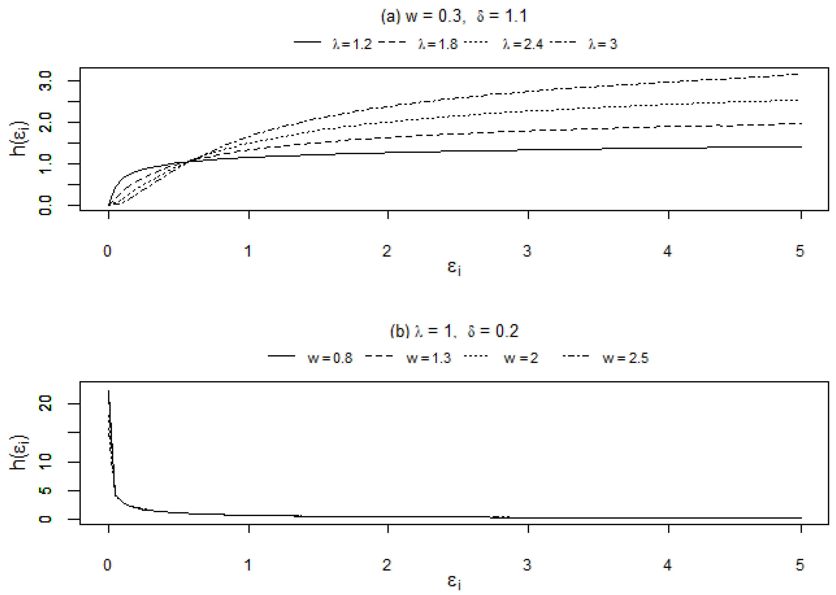
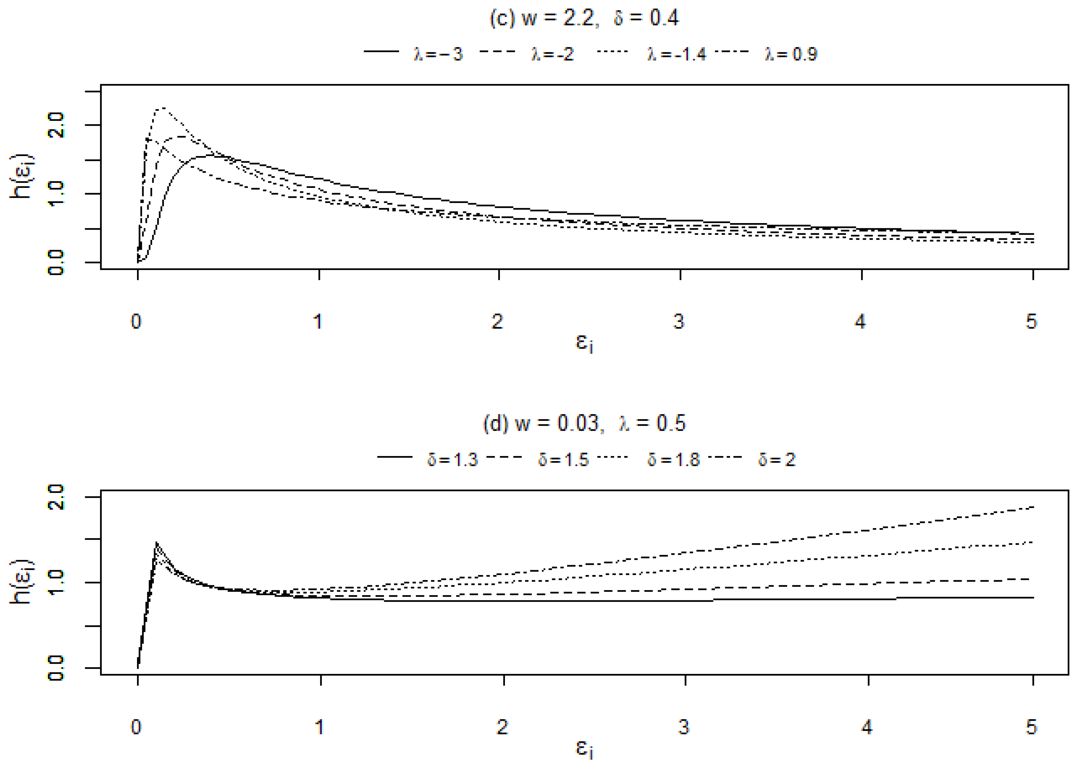
The hazard functions of the standardised EGIG distribution will allow for various shapes such as monotonically increasing (I), monotonically decreasing (D), upside-down bathtub (UB) and upside-down bathtub then bathtub (UBB). Different shapes of the standardised EGIG hazard function can be acquired and subjected to the constraint, $\Delta$, that is

$$\Delta =\{\begin{array}{c}-1, \mathrm{i}\mathrm{f} {\left(\lambda – 1\right)}^2<{\delta }^2\left({\delta }^2-1\right)w^2\\ 0, \mathrm{i}\mathrm{f} {\left(\lambda – 1\right)}^2={\delta }^2\left({\delta }^2-1\right)w^2\\ 1, \mathrm{i}\mathrm{f} {\left(\lambda – 1\right)}^2>{\delta }^2\left({\delta }^2-1\right)w^2\end{array},$$

and other constraints on the distribution parameters as presented in

Table 1. Shapes of hazard function for the standardised EGIG distribution.

Shape	$\Delta$	Other Constraints
I	–1
	0	$\lambda =1$	$\delta >1$
	1	$\lambda <1$	$\delta >1$
	1	$\lambda >1$	$\delta >1$
D	0	$\lambda =1$	$0<\delta <1$
UB	1	$\lambda <1$	$0<\delta <1$
	1	$\lambda >1$	$0<\delta <1$
	1	$\lambda =1$
UBB	1	$\lambda <1$	$\delta >1$

(see [33] for further details). Figure 1 shows the plots for hazard shapes using different sets of parameters with (a) monotonically increasing (I), (b) monotonically decreasing (D), (c) upside-down bathtub (UB) and (d) upside-down bathtub then bathtub (UBB) which consists of more than one turning point.

For illustration purposes, other standardised error distributions were also considered in ACD models, with their respective pdfs and standardisation constraints reflected in

Table 2. Error distributions for ACD models.

Distribution	$\mathbf{pdf},\mathit{f}\left({\mathit{\epsilon }}_{\mathit{i}}\right)$	Mean	Standardisation Constraint
$\mathrm{Wei}(a$$,b$)	$f\left({\epsilon }_i\right)=\frac{a}{b^a}{\epsilon }_i^{a-1}\exp \left[-{\left(\frac{{\epsilon }_i}{b}\right)}^a\right]$	$\mathrm{E}\left({\epsilon }_i\right)=b\mathsf{\Gamma }\left(1+1/a\right)$	$b=\frac{1}{\mathsf{\Gamma }\left(1+1/a\right)}$
$\mathrm{GG}(a$$,b$$,p$)	$f\left({\epsilon }_i\right)=\frac{a}{b^{ap}\mathsf{\Gamma }\left(p\right)}{\epsilon }_i^{ap-1}\exp \left[-{\left(\frac{{\epsilon }_i}{b}\right)}^a\right]$	$\mathrm{E}\left({\epsilon }_i\right)=b\frac{\mathsf{\Gamma }\left(p+1/a\right)}{\mathsf{\Gamma }\left(p\right)}$	$b=\frac{\mathsf{\Gamma }\left(p\right)}{\mathsf{\Gamma }\left(p+1/a\right)}$
$\mathrm{Burr}(a$$,q$$,b$)	$f\left({\epsilon }_i\right)=\frac{aq}{b^a {\left(1+b^{-a}{\epsilon }_i^a\right)}^{1+q}}{\epsilon }_i^{a-1}$	$\mathrm{E}\left({\epsilon }_i\right)=qb\mathrm{B}\left(1+1/a, q-1/a\right)$	$b=\frac{1}{q \mathrm{B}\left(1+1/a, q-1/a\right)}$
$\mathrm{GB}2(a$$,b$$,p$$,q$)	$f\left({\epsilon }_i\right)=\frac{a}{b^{ap}\mathrm{B}\left(p,q\right){\left[1+{\left(\frac{{\epsilon }_i}{b}\right)}^a\right]}^{p+q}}{\epsilon }_i^{ap-1}$	$\mathrm{E}\left({\epsilon }_i\right)=\frac{b\mathrm{B}\left(p+1/a,q-1/a\right)}{\mathrm{B}\left(p,q\right)}$	$b=\frac{\mathrm{B}\left(p,q\right)}{\mathrm{B}\left(p+1/a,q-1/a\right)}$

Remark: $\mathrm{B}\left(·, ·\right)$denotes the beta function and $\mathsf{\Gamma }(·)$ denotes the gamma function.

. Henceforth, the ACD model with any distribution D will be notated as ACD_D.

From Equation (2), the conditional pdf of $x_i$ for the ACD_EGIG(1,1) and CACD_EGIG(1,1) models can be written as

$$f\left(x_i|F_{i-1}\right)=\frac{\delta x_i^{\lambda -1}{\left[K_{\left(\lambda +1\right)/\delta }\left(w\right)\right]}^{\lambda }}{2{\psi }_i^{\lambda } {\left[K_{\lambda /\delta }\left(w\right)\right]}^{\lambda +1}}\exp \left\{-\frac{w}{2}\left[{\left(\frac{x_i K_{\left(\lambda +1\right)/\delta }\left(w\right)}{{\psi }_i K_{\lambda /\delta }\left(w\right)}\right)}^{\delta }+{\left(\frac{x_i K_{\left(\lambda +1\right)/\delta }\left(w\right)}{{\psi }_i K_{\lambda /\delta }\left(w\right)}\right)}^{-\delta }\right]\right\},$$

(18)

i.e., $x_i|F_{i-1}~\mathrm{EGIG}\left(\lambda ,\delta ,{\left[\frac{{\psi }_i{K}_{\lambda /\delta }\left(w\right)}{K_{\left(\lambda +1\right)/\delta }\left(w\right)}\right]}^{\delta },w\right)$.

The corresponding conditional log-likelihood (LL) function is given by

$$\begin{gathered} \mathrm{LL}={{\displaystyle \sum }}_{i=2}^N\ln \left[f\left(x_i|F_{i-1}\right)\right] \\ ={{\displaystyle \sum }}_{i=2}^N\{\ln \left(\delta \right)+\left(\lambda -1\right)\ln \left(x_i\right)+\lambda \ln \left[K_{\left(\lambda +1\right)/\delta }\left(w\right)\right]-\ln \left(2\right)-\lambda \ln \left({\psi }_i\right) \\ -\left(\lambda +1\right)\ln \left[K_{\lambda /\delta }\left(w\right)\right]-\frac{w}{2}\left[{\left(\frac{x_i K_{\left(\lambda +1\right)/\delta }\left(w\right)}{{\psi }_i K_{\lambda /\delta }\left(w\right)}\right)}^{\delta }+{\left(\frac{x_i K_{\left(\lambda +1\right)/\delta }\left(w\right)}{{\psi }_i K_{\lambda /\delta }\left(w\right)}\right)}^{-\delta }\right]\}. \end{gathered}$$

(19)

However, since the initial ${\psi }_1$ is unknown, we set ${\psi }_1=\overline{x}$, where $\overline{x}$ is the sample mean of $x_i.$

From Equation (9), the conditional pdf of $x_i$ for the LogACD_EGIG(1,1) and LogCACD_EGIG(1,1) models can be written as

$$f\left(x_i|F_{i-1}\right)=\frac{\delta x_i^{\lambda -1}{\left[K_{\left(\lambda +1\right)/\delta }\left(w\right)\right]}^{\lambda }}{2e^{\lambda {\psi }_i} {\left[K_{\lambda /\delta }\left(w\right)\right]}^{\lambda +1}}\exp \left\{-\frac{w}{2}\left[{\left(\frac{x_i{K}_{\left(\lambda +1\right)/\delta }\left(w\right)}{e^{{\psi }_i} K_{\lambda /\delta }\left(w\right)}\right)}^{\delta }+{\left(\frac{x_i{K}_{\left(\lambda +1\right)/\delta }\left(w\right)}{e^{{\psi }_i} K_{\lambda /\delta }\left(w\right)}\right)}^{-\delta }\right]\right\},$$

(20)

i.e., $x_i|F_{i-1}~\mathrm{EGIG}\left(\lambda ,\delta ,{\left[\frac{e^{{\psi }_i}{K}_{\lambda /\delta }\left(w\right)}{K_{\left(\lambda +1\right)/\delta }\left(w\right)}\right]}^{\delta },w\right)$.

The corresponding conditional LL function is given by

$$\begin{gathered} \mathrm{LL}={{\displaystyle \sum }}_{i=2}^N\ln \left[f\left(x_i|F_{i-1}\right)\right] \\ ={{\displaystyle \sum }}_{i=2}^N\{\ln \left(\delta \right)+\left(\lambda -1\right)\ln \left(x_i\right)+\lambda \ln \left[K_{\left(\lambda +1\right)/\delta }\left(w\right)\right]-\ln \left(2\right)-\lambda {\psi }_i \\ -\left(\lambda +1\right)\ln \left[K_{\lambda /\delta }\left(w\right)\right]-\frac{w}{2}\left[{\left(\frac{x_i{K}_{\left(\lambda +1\right)/\delta }\left(w\right)}{e^{{\psi }_i} K_{\lambda /\delta }\left(w\right)}\right)}^{\delta }+{\left(\frac{x_i{K}_{\left(\lambda +1\right)/\delta }\left(w\right)}{e^{{\psi }_i} K_{\lambda /\delta }\left(w\right)}\right)}^{-\delta }\right]\}, \end{gathered}$$

(21)

with that ${\psi }_1=\ln \left(\overline{x}\right)$.

For the estimation parts, the maximum likelihood estimates are obtained by maximising the LL functions given by Equations (19) and (21) using the R functions such as gosolnp and optim, where the gosolnp is to find some suitable initial values of the parameters and the optim is utilised in optimisation process. The standard errors of the estimates can then be acquired via the R function such as numericHessian.

4. Data Description

The intra-daily trading times and prices from 3–16 December 2019 in the IBM stock listed on the New York Stock Exchange (NYSE) were retrieved from the Bloomberg Terminal. By removing the data recorded outside the regular operating hours of NYSE, a total of 125,658 transactions were collected from 9:30:00 a.m. to 4:00:00 p.m. and these transactions were treated consecutively from day to day for the calculation of the duration between two consecutive transactions. After filtering out the zero-valued durations and the durations between two consecutive days, a series of 46,288 transactions is obtained. For the given series, we define an event as the IBM stock price changes being greater than or equal to $0.02, which is a similar procedure to that demonstrated by [35]. To be more concrete, we first calculated the duration of each event that occurred and removed the durations between two consecutive days to obtain a series of 7208 durations. The first N = 6633 durations from 3–13 December 2019 were then used for in-sample model fitting, and the one-step-ahead rolling-window technique was used to forecast the out-of-sample duration for h = 575 durations on the next trading day of 16 December 2019.

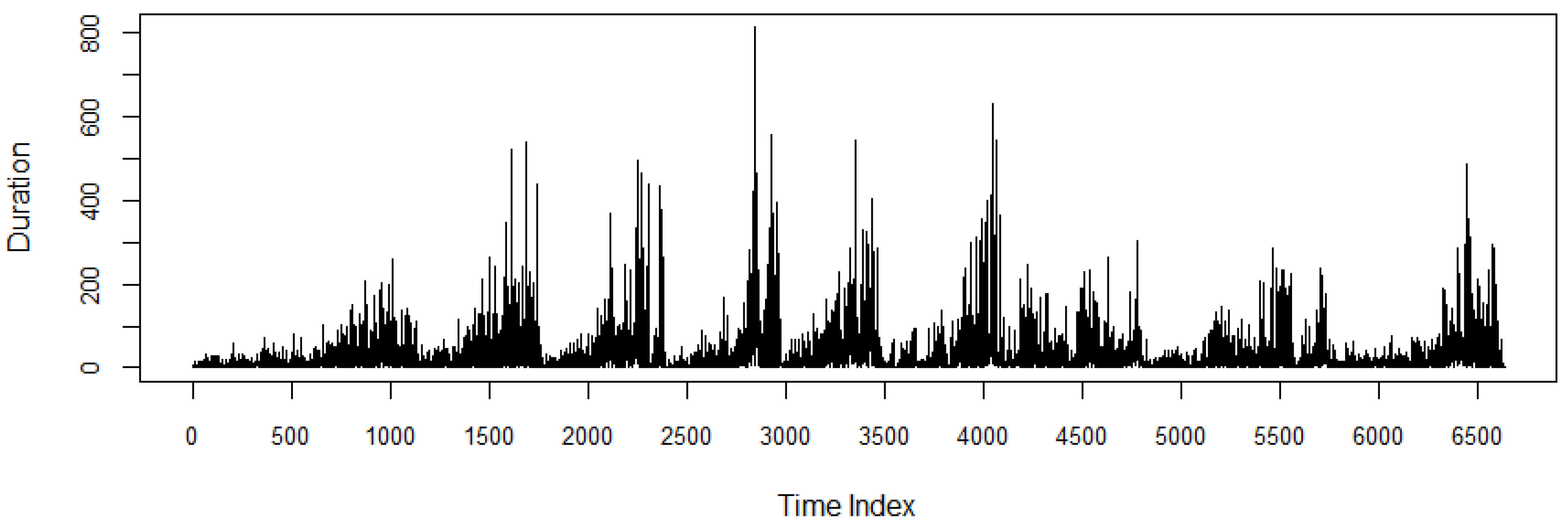
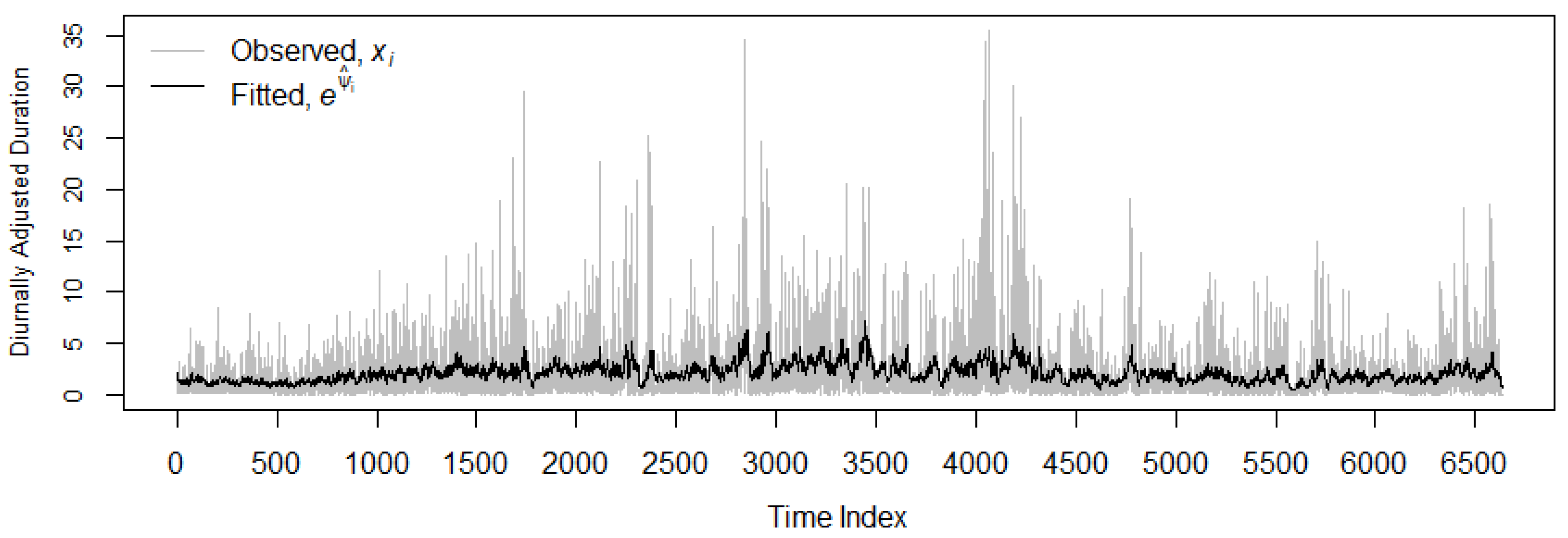
The time series plot of the duration series for the period 3–13 December 2019 is depicted in Figure 2. The graph clearly illustrates that the durations consist of a diurnal pattern, with high trading activities (short duration) at the start and end of each trading day, and low trading activities (long duration) in the middle parts. 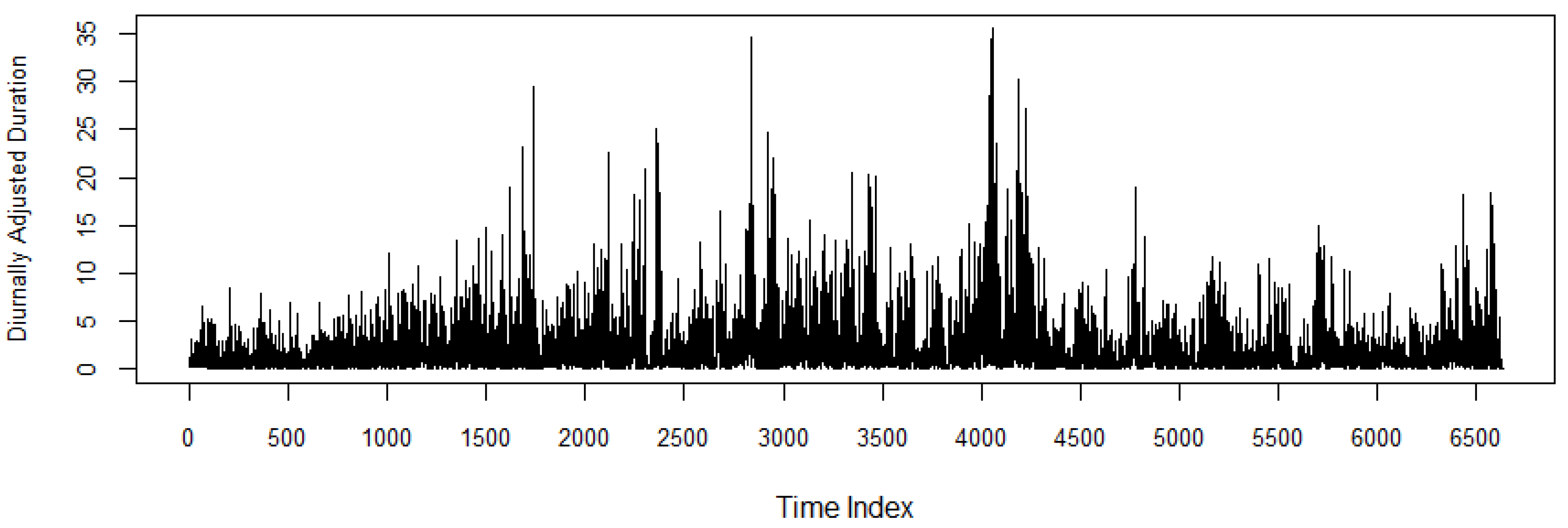By employing the approach that uses the deterministic function (see [29], pp. 253–254) to remove the diurnal effect and obtain the diurnally adjusted duration series by dividing the duration with the fitted deterministic function (see Equation (1)). Figure 3 shows the diurnally adjusted duration series; the summary statistics of the series are reported in

Table 3. Summary statistics of the diurnal adjusted durations from 3–13 December 2019.

Mean	Median	Variance	Skewness	Kurtosis	Min	Max	$\mathit{Q} \left(10\right)$	$\mathit{Q} \left(20\right)$
2.1294	1.1201	8.5131	3.5687	20.4377	0.0361	35.5459	1018.452 *	1591.317 *

* Significance at 1% level.

. The data shows that the durations have an average of 2.1294, with 50% of the diurnally adjusted durations above 1.1201. The skewness of 3.5687 and kurtosis of 20.4377 indicates that the data is positively skewed and has a leptokurtic distribution. Both Ljung-Box (LB) test statistics $Q\left(10\right)$ and $Q\left(20\right)$ at lags 10 and 20, respectively, are significant at 1% significance level, implying a strong autocorrelation in the series.

5. Results and Discussions

5.1. In-Sample Model Fit

The diurnally adjusted durations series using the variations of basic ACD(1,1) models were first modelled as demonstrated by ACD_Wei(1,1), ACD_GG(1,1), ACD_Burr(1,1), ACD_GB2(1,1) and ACD_EGIG(1,1). The results are presented in columns 2 to 6 in

Table 4. Parameter estimates, standard errors (in italic), LL, AIC, BIC, Q_r(10) and Q_r(20) for in-sample estimation of various fitted ACD models.

Parameter	Model
	ACDWei(1,1)	ACDGG(1,1)	ACDBurr(1,1)	ACDGB2(1,1)	ACDEGIG(1,1)	LogACDEGIG(1,1)	CACDEGIG(1,1)	LogCACDEGIG(1,1)
$\vartheta$	0.0487 ***	0.0772 ***	0.0651 ***	0.0772 ***	0.0746 ***	0.0618 ***	-	-
	0.0089	0.0133	0.0116	0.0133	0.0123	0.0069	-	-
${\alpha }_1$	0.0805 ***	0.1010 ***	0.0969 ***	0.1012 ***	0.0791 ***	0.0597 ***	0.0723 ***	0.0710 ***
	0.0071	0.0094	0.0089	0.0094	0.0077	0.0055	0.0083	0.0074
${\beta }_1$	0.8968 ***	0.8652 ***	0.8749 ***	0.8652 ***	0.8852 ***	0.9104 ***	0.8738 ***	0.8750 ***
	0.0095	0.0127	0.0117	0.0127	0.0115	0.0097	0.0147	0.0136
${\omega }_{\mu }$	-	-	-	-	-	-	0.0058 ***	0.0053 ***
	-	-	-	-	-	-	0.0013	0.0003
${\rho }_{\mu }$	-	-	-	-	-	-	0.9972 ***	0.9998 ***
	-	-	-	-	-	-	0.0007	0.0004
${\alpha }_{\mu }$	-	-	-	-	-	-	0.0076 *	0.0072 ***
	-	-	-	-	-	-	0.0038	0.0023
$a$	0.8839 ***	0.3801 ***	1.0157 ***	0.3979 ***	-	-	-	-
	0.0083	0.0308	0.0181	0.0323	-	-	-	-
$p$	-	4.6389 ***	-	4.3432 ***	-	-	-	-
	-	0.7062	-	0.6507	-	-	-	-
$q$	-	-	4.1292 ***	200.0000 **	-	-	-	-
	-	-	0.0181	143.4178	-	-	-	-
$\lambda$	-	-	-	-	0.4040 ***	0.3633 ***	0.4007 ***	0.3592 ***
	-	-	-	-	0.0303	0.0305	0.0297	0.0270
$\delta$	-	-	-	-	1.0604 ***	1.0399 ***	1.0833 ***	1.0849 ***
	-	-	-	-	0.0544	0.0544	0.0552	0.0446
$w$	-	-	-	-	0.2328 ***	0.2595 ***	0.2169 ***	0.2230 ***
	-	-	-	-	0.0395	0.0441	0.0372	0.0309
LL	−11,083.35	−10,973.99	−11,037.85	−10,975.21	−10,895.97	−10,890.23	−10,889.74	−10,878.35
AIC	22,174.71	21,957.97	22,085.70	21,962.43	21,803.94	21,792.45	21,795.49	21,772.69
BIC	22,201.91	21,991.97	22,119.70	22,003.23	21,844.74	21,833.25	21,849.89	21,827.09
Qr(10)	12.1400	16.6061 *	16.1375 *	16.6614 *	11.5349	49.5479 ***	12.2383	18.2597 *
Qr(20)	19.1207	23.6021	23.0540	23.6568	19.0005	67.7134 ***	20.5359	27.2273

Note: Q_r(m) is the LB test statistic at lag m of the standardised residuals. *** Significance at 1% level; ** Significance at 5% level; * Significance at 10% level.

. Among those basic ACD(1,1) models, the ACD_EGIG(1,1) model is chosen as the best-fitted model with the largest LL of −10895.97, and the smallest Akaike information criterion (AIC) and Bayesian information criteria (BIC) of 21803.94 and 21844.74, respectively. We further examine the estimated parameters of the models, we observe that (i) the ACD_Wei(1,1) model with $\widehat{a}<1$ indicates a monotonically decreasing (D) hazard function, (ii) the ACD_GG(1,1) model with $\left(\widehat{a}\widehat{p} –1\right)>0$ and $\widehat{a}<1$ has a upside-down-bathtub (UB) hazard function, (iii) the ACD_Burr(1,1) model with $\widehat{a}>1$ and $\left(\widehat{a}\widehat{p} –1\right)>0$gives a UB hazard function, and (iv) the ACD_GB2(1,1) model with $\left(\widehat{a}\widehat{p} –1\right)>0$, $\widehat{a}<1$ and $\widehat{p}<\frac{2}{\widehat{a}\left(\widehat{a}+1\right)}-\frac{\left(\widehat{a}-1\right)\widehat{q}}{\left(\widehat{a}+1\right)}$ implies a UB hazard function. However, the ACD_EGIG(1,1) model with $\widehat{\lambda }<1$, $\widehat{\delta }>1$, $\widehat{w}>0$ and ${\left(\widehat{\lambda } – 1\right)}^2>{\widehat{\delta }}^2\left({\widehat{\delta }}^2-1\right){\widehat{w}}^2$ indicates that the hazard function has more than one turning point with upside-down bathtub then bathtub (UBB) shape. In addition, the estimates of ${\widehat{\alpha }}_1+{\widehat{\beta }}_1$ = 0.9643 from the ACD_EGIG(1,1) model possesses the greatest distance from one as compared to other basic ACD(1,1) models, which indicates the EGIG distribution indeed helps to capture the persistency of duration. The LB test statistics of the standardised residuals for all basic ACD(1,1) models are not significant at lags 10 and 20 at 5% significance level. Meanwhile, the autocorrelation function (ACF) plots of these models are presented in Figure 4a–e, which confirm that the standardised residuals of the fitted models have no (weak) serial correlations.

Subsequently, the modelling performance of the ACD model with linear mean specification, ACD_EGIG(1,1) and the ACD models with nonlinear mean specifications, LogACD_EGIG(1,1) and CACD_EGIG(1,1) models (refer to columns 7 and 8 in Table 4) were compared. It can be noted that the nonlinear models tend to produce a better model fit than the linear model, in which case the LogACD_EGIG(1,1) model gives the smallest AIC and BIC. However, the LB test statistics of the standardised residuals for the LogACD_EGIG(1,1) model are significant at lags 10 and 20 at 1% significance level which indicate that the series is highly autocorrelated. The corresponding ACF plot is illustrated in Figure 4f. This result is in line with the finding of [4] that the LogACD model is unable to capture the long memory effect of IBM trade duration series.

Lastly, in overall comparison among all the models, the LogCACD_EGIG(1,1) model offers the best fit with the largest LL and smallest AIC and BIC as highlighted in boldface in Table 4. Figure 5 demonstrates the fitted duration series of the LogCACD_EGIG(1,1) model superimposed on the observed series while Figure 6 plots the fitted $e^{{\widehat{\psi }}_i}$, $e^{{\widehat{\psi }}_{i,1}}$ and $e^{{\widehat{\psi }}_{i,2}}$ series of the LogCACD_EGIG(1,1) model. It is worth noting that the estimated model parameters also satisfy the UBB constraints, which confirm the presence of the UBB-shaped hazard function. Moreover, ${\widehat{\rho }}_{\mu }$ and ${\widehat{\alpha }}_1+{\widehat{\beta }}_1$ of the model suggests that the decay rates of the short-run component and long-run component are well-separated, with the short-run component having a faster mean-reverting rate than the long-run component. To put it simply, the long-run component is more persistent than the short-run component with $0<\left({\widehat{\alpha }}_1+{\widehat{\beta }}_1\right)<{\widehat{\rho }}_{\mu }<1$. With ${\widehat{\alpha }}_1>{\widehat{\alpha }}_{\mu }$, the model establishes a greater immediate impact on the short-run component than on the long-run component. To ease depiction, Figure 4g,h display the ACF plots of standardised residuals for the CACD_EGIG(1,1) and LogCACD_EGIG(1,1) models, respectively, with the LB tests at lags 10 and 20 showing they are not significant at 5% significance level. This implies that the component LogCACD_EGIG(1,1) model has managed to remove the autocorrelation in the IBM trade duration series as compared to the LogACD_EGIG(1,1) model.

5.2. Out-of-Sample Forecasts

Essentially, the ability to generate accurate forecasts of trade durations is of utmost importance in practice. Thus, we implement the one-step ahead rolling window technique to forecast $h=575$ points on 16 December 2019. To remove the diurnal effect, for each window, we fit the duration series to a deterministic function and calculate the diurnally adjusted durations series using Equation (1). The resulting adjusted series was then fitted with the ACD models to obtain the one-step ahead forecast while the one-step ahead “observed” adjusted duration was acquired by dividing the observed duration with the fitted deterministic function.

For assessing the forecasting ability among competing duration models, the forecast errors were computed based on several loss functions.

Table 5. Comparison of forecast errors using MSFE and QLIKE.

Model	MSFE	QLIKE
ACDWei(1,1)	10.8131	0.7378
ACDGG(1,1)	10.8663	0.7375
ACDBurr(1,1)	10.8601	0.7377
ACDGB2(1,1)	10.8674	0.7375
ACDEGIG(1,1)	10.7880	0.7366
LogACDEGIG(1,1)	10.7842	0.7408
CACDEGIG(1,1)	10.7583	0.7324
LogCACDEGIG(1,1)	10.7522	0.7330

Note: MSFE = $\frac{1}{h}{\displaystyle \sum }_{i=N+1}^{N+h}{\left(x_i-{\widehat{x}}_i\right)}^2$ and QLIKE = $\frac{1}{h}{\displaystyle \sum }_{i=N+1}^{N+h}\left[\frac{x_i}{{\widehat{x}}_i}-\ln \left(\frac{x_i}{{\widehat{x}}_i}\right)-1\right]$.

reports the results of mean square forecast error (MSFE) and quasi-likelihood (QLIKE) for eight ACD models. On the basis of MSFE, the LogCACD_EGIG(1,1) model appears to be the best forecasting model among those considered models. However, the CACD_EGIG(1,1) model is the most favourable by means of QLIKE estimate and the LogCACD_EGIG(1,1) model is still the second best.

Meanwhile, the MCS procedure was employed to test the equal predictive ability among all the models at a certain fixed confidence level, and the SSM was then generated. The MCS procedure was implemented via the R function of MCSprocedure() and evaluated using 5000 bootstrap replications tested at a 95% confidence level (see [36]). The rank and p-values of the MCS procedure using the loss functions, MSFE and QLIKE, are listed in

Table 6. Comparison of forecasting performance based on MCS procedure with MSFE as loss function.

Model	Rank	p-value
LogCACDEGIG(1,1)	1	1.0000
CACDEGIG(1,1)	2	1.0000
LogACDEGIG(1,1)	3	0.8916
ACDEGIG(1,1)	4	0.2906
ACDWei(1,1)	5	0.1236

Models eliminated: ACD_GG(1,1), ACD_Burr(1,1) and ACD_GB2(1,1).

and

Table 7. Comparison of forecasting performance based on MCS procedure with QLIKE as loss function.

Model	Rank	p-value
CACDEGIG(1,1)	1	1.0000
LogCACDEGIG(1,1)	2	1.0000
ACDWei(1,1)	3	0.6244
ACDGB2(1,1)	4	0.5318
ACDBurr(1,1)	5	0.5304
ACDGG(1,1)	6	0.5258
ACDEGIG(1,1)	7	0.5248
LogACDEGIG(1,1)	8	0.4742

Models eliminated: None.

. Results in Table 6 reveal that all ACD models with EGIG distribution are not eliminated during the process, implying that the EGIG distribution is capable of describing the shape and the dynamics of the IBM trade durations. Among these models, nonlinear ACD models are ranked first through third with the LogCACD_EGIG(1,1) model having the highest rank. On the other hand, none of the models are eliminated through the MCS procedure using QLIKE loss function (see Table 7). The CACD_EGIG(1,1) and LogCACD_EGIG(1,1) models are ranked first and second, respectively, in SSM. Hence, we are of the view that the two-component ACD models seem to have a better predicting power than the one-component ACD models.

5.3. TaR Forecasts

As for the risk analysis part, the one-step ahead forecast of TaR is used to evaluate the liquidity risk of trade duration. The $100\left(1-u\right)\%$ upper limit i-th TaR forecast of the ACD_EGIG(1,1) and CACD_EGIG(1,1) models is given by

$${\mathrm{TaR}}_{i,1-u}={\psi }_i{\left(\frac{2z}{w}\right)}^{1/\delta }\frac{K_{\lambda /\delta }\left(w\right)}{K_{\left(\lambda +1\right)/\delta }\left(w\right)},i=N+1,N+2, \dots ,N+h,$$

(22)

where $u$ is the upper risk level, while the $100\left(1-u\right)\%$ upper limit i-th TaR forecast for the LogACD_EGIG(1,1) and LogCACD_EGIG(1,1) models is given by

$${\mathrm{TaR}}_{i,1-u}=e^{{\psi }_i}{\left(\frac{2z}{w}\right)}^{1/\delta }\frac{K_{\lambda /\delta }\left(w\right)}{K_{\left(\lambda +1\right)/\delta }\left(w\right)},i=N+1,N+2, \dots ,N+h,$$

(23)

where the $z$ in both Equations (22) and (23) are the solution of

$${{\displaystyle \int }}_0^z{t}^{\lambda /\delta -1}\exp \left(-t-\frac{w^2}{4}{t}^{-1}\right)dt=2\left(1-u\right){\left(\frac{w}{2}\right)}^{\lambda /\delta }{K}_{\lambda /\delta }\left(w\right).$$

(24)

The derivations of ${\mathrm{TaR}}_{i,1-u}$ indicated by Equations (22) and (23) are shown in the Appendix A.

Table 8. ${\mathrm{TaR}}_{i,1-u}$ for basic ACD(1,1) model under different distributions.

Model	$\mathbf{T}\mathbf{a}{\mathbf{R}}_{\mathit{i},1-\mathit{u}}$
ACDWei(1,1)	$\frac{{\psi }_i}{\mathsf{\Gamma }\left(1+1/a\right)}{\left[-\ln \left(u\right)\right]}^{\frac{1}{a}}$
ACDGG(1,1)	$\frac{{\psi }_i\mathsf{\Gamma }\left(p\right)}{\mathsf{\Gamma }\left(p+1/a\right)}{z}^{\frac{1}{a}}$, where $z$ is the solution of ${{\displaystyle \int }}_0^z{t}^{p-1}\exp \left(-t\right)dt=\left(1-u\right)\mathsf{\Gamma }\left(p\right)$
ACDBurr(1,1)	$\frac{{\psi }_i}{q \mathrm{B}\left(1+1/a, q-1/a\right) }{\left[u^{-\frac{1}{q}}-1\right]}^{\frac{1}{a}}$
ACDGB2(1,1)	$\frac{{\psi }_i\mathrm{B}\left(p,q\right)}{\mathrm{B}\left(p+1/a,q-1/a\right)}{\left[\frac{z}{1-z}\right]}^{\frac{1}{a}}$, where $z$ is the solution of ${{\displaystyle \int }}_0^z{t}^{p-1}{\left(1-t\right)}^{q-1}dt=\left(1-u\right)\mathrm{B}\left(p,q\right)$

provides the $100\left(1-u\right)\%$ upper limit TaR forecasts for various basic ACD(1,1) models under different distributions.

In order to assess the quality of TaR forecasts, the model should always be backtested with appropriate statistical tools. Amongst these, the violation rate (VR) for the upper quantile is computed as

$${\nu }_u=\frac{n_u}{h}=\frac{1}{h}{{\displaystyle \sum }}_{i=N+1}^{N+h}\mathrm{I}\left(x_i>{\mathrm{TaR}}_{i,1-u}\right),$$

(25)

where $n_u$ is an estimate of the number of TaR violations at the upper risk level $u$ and $\mathrm{I}(·)$ represents an indicator function. The ratio of VR, ${\mathrm{RVR}}_u=\frac{{\nu }_u}{u}$, indicates an agreement between ${\nu }_u$ and $u$ in which the ratio equals one implies a complete agreement.

Table 9. Risk performance measures for one-step-ahead TaR forecasts and the p-values of KLR test at upper risk levels 0.025, 0.05 and 0.10 using various ACD models.

Model	$\mathit{u}$
	0.025			0.05			0.10
	${\mathit{\nu }}_{\mathit{u}}$	$\mathbf{R}\mathbf{V}{\mathbf{R}}_{\mathit{u}}$	p-value of KLR Test	${\mathit{\nu }}_{\mathit{u}}$	$\mathbf{R}\mathbf{V}{\mathbf{R}}_{\mathit{u}}$	p-value of KLR Test	${\mathit{\nu }}_{\mathit{u}}$	$\mathbf{R}\mathbf{V}{\mathbf{R}}_{\mathit{u}}$	p-value of KLR Test
ACDWei(1,1)	0.0313	1.2522	0.3512	0.0626	1.2522	0.1812	0.1357	1.3565	0.0066 ***
ACDGG(1,1)	0.0226	0.9043	0.7090	0.0574	1.1478	0.4264	0.1322	1.3217	0.0138 **
ACDBurr(1,1)	0.0243	0.9739	0.9199	0.0626	1.2522	0.1812	0.1426	1.4261	0.0013 ***
ACDGB2(1,1)	0.0226	0.9043	0.7090	0.0574	1.1478	0.4264	0.1322	1.3217	0.0138 **
ACDEGIG(1,1)	0.0261	1.0435	0.8683	0.0574	1.1478	0.4264	0.1270	1.2696	0.0378 **
LogACDEGIG(1,1)	0.0330	1.3217	0.2387	0.0609	1.2174	0.2468	0.1304	1.3043	0.0195 **
CACDEGIG(1,1)	0.0261	1.0435	0.8683	0.0591	1.1826	0.3283	0.1252	1.2522	0.0515 *
LogCACDEGIG(1,1)	0.0278	1.1130	0.6698	0.0557	1.1130	0.5410	0.1252	1.2522	0.0515 *

*** Significance at 1% level; ** Significance at 5% level; * Significance at 10% level.

reports the ${\nu }_u$ and ${\mathrm{RVR}}_u$ of TaR forecasts for upper risk levels of 0.025, 0.05 and 0.10. It should be noted that all the estimated ${\nu }_u$ values are in line with their respective risk levels of the models, particularly the TaR values based on the LogCACD_EGIG(1,1) model. These values have the closest ${\nu }_u$ values to its target risk levels as well as the ${\mathrm{RVR}}_u$ values having the smallest deviation from the value of one for risk levels of 0.05 and 0.10, indicating a close agreement between observed durations and TaR forecasts.

Apart from these measures, the KLR test was also carried out to evaluate the accuracy of the estimated TaR. Let the number of TaR violations $n_u$ follow a binomial distribution with $h$ trials and success probability $u$. [26] proposed a likelihood ratio (LR) test statistic as

$$\mathrm{LR}=-2\ln \left[u^{n_u}{\left(1 – u\right)}^{h-n_u}\right]+2\ln \left[{\left(n_u/h\right)}^{n_u}{\left(1 –\left(n_u/h\right)\right)}^{h-n_u}\right] \text{~} {\chi }_1^2,$$

(26)

where ${\chi }_1^2$ denotes a chi-squared distribution with one degree of freedom under the null hypothesis that TaR model is correctly specified. The p-values of the KLR test are reported in Table 9 and the findings show insufficient evidence to reject the null hypothesis for the upper risk levels 0.025 and 0.05 for all ACD models at 10% significance level. However, only the TaR forecasts based on the CACD_EGIG(1,1) and LogCACD_EGIG(1,1) at upper risk level 0.10 are not rejected at 5% significance level, implying that these two models provide more precise TaR forecasts. For the sake of illustration, Figure 7 plots the TaR upper limits at 90%, 95% and 97.5% using the LogCACD_EGIG(1,1) model together with its observed durations and it can be observed that the TaR forecasts at various levels are quite capable of capturing the trend of the observed durations well.

6. Conclusions

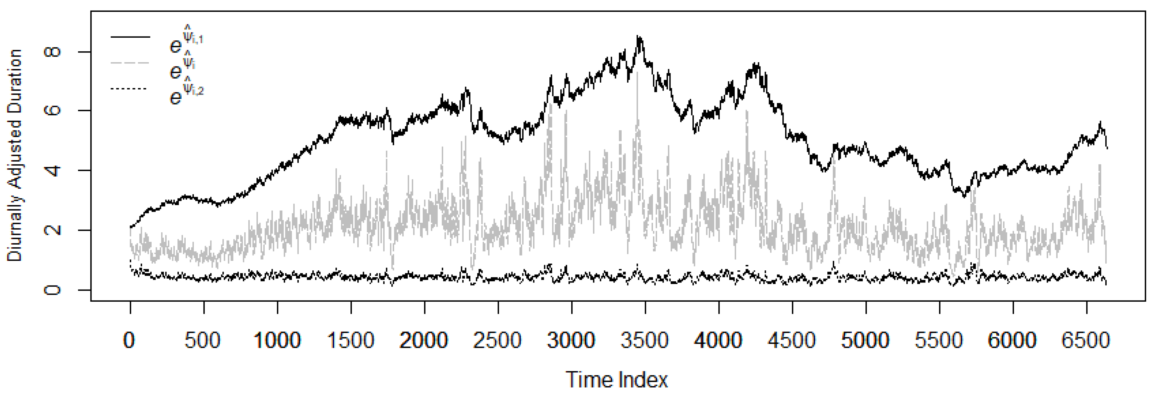
Generally, this paper proposes a novel model called the LogCACD model with no restrictions on the sign of parameters while allowing the expected durations to be decomposed into the long- and short-run components in duration modelling. The aggregation of long- and short-run components leads to a slowly decaying autocorrelation that closely resembles the one observed on trade duration data. We first analysed the goodness of fit of the proposed LogCACD model with three different linear and nonlinear benchmark models, namely ACD, LogACD and CACD for capturing the dynamics of trade durations in terms of their in-sample model-fit and out-of-sample forecast performances. It was then followed by the investigation of the effect of different distribution assumptions for these models, in which a flexible EGIG error distribution with a roller-coaster shaped hazard function was adopted and compared the performance with the Wei, GG, Burr and GB2 error distributions. Finally, for risk measure analysis, the TaR forecasts were computed and evaluated using various performance measures and backtests.

Meanwhile, an empirical application based on IBM trade durations with the preliminary comparison of the in-sample model fit was carried out using the basic linear ACD models under different error distributions. The findings reveal that the ACD_EGIG offers the best model fit and all the estimated parameters fulfil the constraints of the UBB-shaped hazard function (see Table 1) highlighting the practical advantage of the EGIG distribution as a potential error distribution for ACD modelling. In addition, the linear and nonlinear ACD models were contrasted with the EGIG distribution, and the result appears to warrant the conclusion that the LogCACD_EGIG model tends to outperform the other models, which indicates that the choices of mean specifications and error distributions turn out to be the important factors for improving modelling performance of trade duration.

To further examine the applications of nonlinear mean specifications and EGIG distribution for enhancing the duration forecasts, the forecasting performance of these models was evaluated via loss functions, namely MSFE and QLIKE and tested using the MCS test. The LogCACD_EGIG model seems to provide the smallest and the second smallest ranks based on MSFE and QLIKE, respectively, and the MCS test procedure also confirms the predictive ability of LogCACD_EGIG model in producing precise forecasts. Concurrently, the computed TaR forecasts of these models were evaluated to assess the forecast accuracy and the results appear to show that the TaR forecasts based on LogCACD_EGIG model at all risk levels are reasonably reflected in terms of the ratio of violation rates. The KLR test is also in line with the accuracy of the TaR forecasts.

As a summary, it is worth noting that the LogCACD model with nonlinear mean specification and a flexible EGIG distribution tends to improve the trade durations forecasting performance under study. For illustration purposes, assuming that there are only two types of traders in the market constituted by the uninformed and informed traders. Our proposed component model could be used to explain the trade behaviour of these traders. Both the long- and short-run components represent the uninformed and informed trader’s trade duration, respectively. The long-run component exhibits highly persistent behaviour, which supports the hypothesis that the uninformed trader acquires the delay trading information from the informed trader. This result is in line with the finding of [37], that uninformed trade responds more to past uninformed trade than it does to past informed trade. Despite the encouraging results of this study, the change of durations might also be affected by other market events such as price and volume. Hence, in future works, it would be interesting to extend our model by incorporating other exogenous variables such as transaction volume, trading intensity and spread associated with trade duration to improve the predictive ability. Moreover, it would be meaningful to consider the application of EGIG distribution in stochastic conditional duration models which can account for the structural change exhibited by the durations.

References

1. Easley, D.; Kiefer, N.M.; O’hara, M.; Paperman, J.B. Liquidity, information, and infrequently traded stocks. J. Financ. 1996, 51, 1405–1436. [Google Scholar] [CrossRef]
2. Engle, R.F.; Russell, J.R. Autoregressive conditional duration: A new model for irregularly spaced transaction data. Econometrica 1998, 66, 1127–1162. [Google Scholar] [CrossRef]
3. Lunde, A. A Generalized Gamma Autoregressive Conditional Duration Model; Working Paper; Department of Economics, Politics and Public Administration, Aalborg University: Copenhagen, Denmark, 1999. [Google Scholar]
4. Bauwens, L.; Giot, P. The logarithmic ACD model: An application to the bid-ask quote process of three NYSE stocks. Ann. D’Economie Stat. 2000, 60, 117–149. [Google Scholar] [CrossRef]
5. Jasiak, J. Persistence in Intertrade Durations. 1999. Available online: https://ssrn.com/abstract=162008 (accessed on 8 November 2021).
6. Zhang, M.Y.; Russell, J.R.; Tsay, R.S. A nonlinear autoregressive conditional duration model with applications to financial transaction data. J. Econom. 2001, 104, 179–207. [Google Scholar] [CrossRef]
7. Bauwens, L.; Giot, P. Asymmetric ACD models: Introducing price information in ACD models. Empir. Econ. 2003, 28, 709–731. [Google Scholar] [CrossRef]
8. Fernandes, M.; Grammig, J. A family of autoregressive conditional duration models. J. Econom. 2006, 130, 1–23. [Google Scholar] [CrossRef] [Green Version]
9. Pacurar, M. Autoregressive conditional duration models in finance. A survey of the theoretical and empirical literature. J. Econ. Surv. 2008, 22, 711–751. [Google Scholar] [CrossRef]
10. Hautsch, N. Econometrics of Financial High-Frequency Data, 1st ed.; Springer: New York, NY, USA, 2012. [Google Scholar]
11. Bhogal, S.K.; Variyam, R.T. Conditional duration models for high-frequency data: A review on recent developments. J. Econ. Surv. 2019, 33, 252–273. [Google Scholar] [CrossRef] [Green Version]
12. Engle, R.F. The econometrics of ultra-high-frequency data. Econometrica 2000, 68, 1–22. [Google Scholar] [CrossRef] [Green Version]
13. Huang, Z.; Han, A.; Wang, S. Component ACD model and its application in studying the price-related feedback effect in investor trading behaviors in Chinese stock market. J. Syst. Sci. Complex. 2018, 31, 677–695. [Google Scholar] [CrossRef]
14. Grammig, J.; Maurer, K.O. Non-monotonic hazard functions and the autoregressive conditional duration model. Econom. J. 2000, 3, 16–38. [Google Scholar] [CrossRef]
15. Hautsch, N. Assessing the risk of liquidity suppliers on the basis of excess demand intensities. J. Financ. Econom. 2003, 1, 189–215. [Google Scholar] [CrossRef]
16. De Luca, G.; Zuccolotto, P. Regime-switching Pareto distributions for ACD models. Comput. Stat. Data Anal. 2006, 51, 2179–2191. [Google Scholar] [CrossRef]
17. Xu, Y. The Lognormal Autoregressive Conditional Duration (LNACD) Model and a Comparison with an Alternative ACD Models. 2013. Available online: https://ssrn.com/abstract=2382159 (accessed on 7 October 2021).
18. Yatigammana, R.P.; Choy, S.T.B.; Chan, J.S.K. Autoregressive conditional duration model with an extended Weibull error distribution. In Causal Inference in Econometrics; Springer: Berlin/Heidelberg, Germany, 2016; pp. 83–107. [Google Scholar]
19. Zheng, Y.; Li, Y.; Li, G. On Fréchet autoregressive conditional duration models. J. Stat. Plan. Inference 2016, 175, 51–66. [Google Scholar] [CrossRef] [Green Version]
20. Bień-Barkowska, K. Extension and verification of the asymmetric autoregressive conditional duration models. Int. J. Comput. Math. 2017, 94, 2223–2238. [Google Scholar] [CrossRef]
21. Yatigammana, R.P.; Chan, J.S.K.; Gerlach, R.H. Forecasting trade durations via ACD models with mixture distributions. Quant. Financ. 2019, 19, 2051–2067. [Google Scholar] [CrossRef]
22. Allen, D.; Chan, F.; McAleer, M.; Peiris, S. Finite sample properties of the QMLE for the Log-ACD model: Application to Australian stocks. J. Econom. 2008, 147, 163–185. [Google Scholar] [CrossRef] [Green Version]
23. Bień-Barkowska, K. Distribution choice for the asymmetric ACD models. Dyn. Econom. Models 2011, 11, 55–72. [Google Scholar] [CrossRef] [Green Version]
24. Ng, K.H.; Shelton, P. Modelling high frequency transaction data in financial economics: A comparative study based on simulations. Econ. Comput. Econ. Cybern. Stud. Res. 2013, 47, 189–201. [Google Scholar]
25. Ghysels, E.; Gouriéroux, C.; Jasiak, J. Stochastic volatility duration models. J. Econom. 2004, 119, 413–433. [Google Scholar] [CrossRef]
26. Kupiec, P.H. Techniques for verifying the accuracy of risk measurement models. J. Deriv. 1995, 3, 73–84. [Google Scholar] [CrossRef]
27. Christoffersen, P.F. Evaluating interval forecasts. Int. Econ. Rev. 1998, 39, 841–862. [Google Scholar] [CrossRef]
28. Hansen, P.R.; Lunde, A.; Nason, J.M. The model confidence set. Econometrica 2011, 79, 453–497. [Google Scholar] [CrossRef] [Green Version]
29. Tsay, R.S. Analysis of Financial Time Series, 3rd ed.; John Wiley & Sons: Hoboken, NJ, USA, 2010. [Google Scholar]
30. Engle, R.F.; Lee, G.G.J. A long-run and short-run component model of stock return volatility. In Cointegration, Causality and Forecasting: A Festschrift in Honor of Clive W. J. Granger; Engle, R.F., White, H., Eds.; Oxford University Press: Oxford, UK, 1999; pp. 475–497. [Google Scholar]
31. Silva, R.S.; Lopes, H.F.; Migon, H.S. The extended generalized inverse Gaussian distribution for log-linear and stochastic volatility models. Braz. J. Probab. Stat. 2006, 20, 67–91. [Google Scholar]
32. Shakil, M.; Kibria, B.M.G.; Singh, J.N. A new family of distributions based on the generalized Pearson differential equation with some applications. Austrian J. Stat. 2010, 39, 259–278. [Google Scholar] [CrossRef]
33. Gupta, R.C.; Viles, W. Roller-coaster failure rates and mean residual life functions with application to the extended generalized inverse Gaussian model. Probab. Eng. Inf. Sci. 2011, 25, 103–118. [Google Scholar] [CrossRef]
34. Gupta, R.C.; Viles, W. Statistical inference for the extended generalized inverse Gaussian model. J. Stat. Comput. Simul. 2012, 82, 1855–1872. [Google Scholar] [CrossRef]
35. Cheung, L. High Frequency Data: Modeling Durations via the ACD and Log ACD Models. Honours Scholar Theses, University of Connecticut, Storrs, CT, USA, 2014; p. 394. [Google Scholar]
36. Bernardi, M.; Catania, L. The model confidence set package for R. Int. J. Comput. Econ. Econom. 2018, 8, 144–158. [Google Scholar] [CrossRef]
37. Easley, D.; Engle, R.F.; O’Hara, M.; Wu, L. Time-varying arrival rates of informed and uninformed trades. J. Financ. Econom. 2008, 6, 171–207. [Google Scholar]
Figure 1. Hazard functions of the standardised EGIG distribution with different sets of distribution parameters.
Mathematics 10 01621 g001aMathematics 10 01621 g001b
Figure 2. Time series plot of the durations after demarcated IBM stock price change greater or equal to $0.02.
Mathematics 10 01621 g002
Figure 3. Time series plot of the diurnally adjusted durations from 3–13 December 2019.
Mathematics 10 01621 g003
Figure 4. ACF plots for the standardised residuals of the fitted models.
Mathematics 10 01621 g004
Figure 5. Observed and fitted series using LogCACDEGIG(1,1) model from 3–13 December 2019.
Mathematics 10 01621 g005
Figure 6. Fitted e ψ ^ i , e ψ ^ i , 1 and e ψ ^ i , 2 series using LogCACDEGIG(1,1) model from 3–13 December 2019.
Mathematics 10 01621 g006
Figure 7. Observed values and TaR forecasts for different upper levels of 90%, 95% and 97.5% using the LogCACDEGIG(1,1) model.
Mathematics 10 01621 g007