Predicting Time SeriesUsing an Automatic New Algorithm of the Kalman Filter

Abstract

Time series forecasting is one of the main venues followed by researchers in all areas. For this reason, we develop a new Kalman filter approach, which we call the alternative Kalman filter. The search conditions associated with the standard deviation of the time series determined by the alternative Kalman filter were suggested as a generalization that is supposed to improve the classical Kalman filter. We studied three different time series and found that in all three cases, the alternative Kalman filter is more accurate than the classical Kalman filter. The algorithm could be generalized to time series of a different length and nature. Therefore, the developed approach can be used to predict any time series of data with large variance in the model error that causes convergence problems in the prediction.

1. Introduction

Forecasting has become one of the main objectives on which many researchers around the world focus their efforts. Advances in computing and the ease of collecting and storing large time series contribute to the development of predictive models in countless areas. This is because good forecast accuracy can improve decision making and planning in each of these areas.

The approaches to time series forecasting are basically divided into single-factor and multi-factor time series models. The former considers time as the unique independent variable and builds mathematical models to produce predictions about the future; the latter also takes into account other factors that influence the system.

External factors, such as prices, costs, crop management, consumer behavior or weather conditions, often require economic and demographic data that may not be available or that are difficult to obtain, in addition to the need to make predictions regarding how these factors will affect the accuracy of the production predictions. Therefore, it is worth considering, in the first instance, whether single-factor models offer sufficiently accurate predictions.

One of the most applied methods for forecasting, especially in the field of time series, is ARIMA (autoregressive integrated moving average), which consists of a linear predictive system that is applied to time series, offering, so far, good predictive results in the short term in different areas [1,2,3,4,5,6,7]. Thus, our first objective is to generate fast and reliable forecasts produced only from the time series, with time considered as the unique independent variable, developing an algorithm that automatically identifies the optimal ARIMA components.

Another method widely used in predictive models is the Kalman filter, which is applied to dynamic systems in the state space to predict the state of a system from previous states. This algorithm is based on an the a priori prediction of the state of a system at an instant t from its previous states, to make a subsequent correction that refines the result. As with other time series models, the Kalman filter includes a stochastic component that is responsible for the dispersion of the prediction but, in this case, the stochastic component does not act only as a summation element, but rather forms part of the algorithm, and its value must be computationally simulated for the instant we want to predict. Therefore, a large variance in the model error would cause a large distortion in the prediction. However, for stable time series without large variability, we can find some recent examples in which the Kalman filter is used to predict [8,9,10,11,12,13,14]. Moreover, it usually appears combined with ARIMA, as can be seen in recent studies applied to different areas [15,16,17,18].

The situation described above about the convergence problems of the Kalman filter due to the excessively large standard deviation of the noise associated with the process have been systematically avoided by several authors. Our second and relevant contribution in this work is to propose a possible solution that solves the convergence problems of the classical Kalman filter. Therefore, following the hypotheses of the classical Kalman filter and, in order to increase the predictive reliability of time series in different fields, we develop a new hybrid process with the Kalman filter, which we will call the alternative Kalman filter, to include the ARIMA model in the state space.

We can find similar approaches to this in autoregression (AR) processes [19,20,21,22], but the main advantage of AR is that it uses only the time series and the system error. In this paper, we try to prove that we can obtain a good prediction without the need for other variables or complex algorithms, such as machine learning process or neural networks, and also improve the results obtained by the classical Kalman filter.

The performance of the new algorithm is evaluated in accordance with usual error metrics commonly employed to assess forecasting models [1,4,5,8,10,14,23], such as root mean squared error (RMSE), mean absolute error (MAE), symmetric mean absolute percentage error (sMAPE), mean absolute scaled error (MASE), and some other metrics, such as the Akaike information criteria (AIC) and Bayesian information criteria (BIC), as well as the goodness of fit of the model through the $R_{\mathrm{adjusted}}^2$.

In addition to the descriptive criteria, the modified Diebold and Mariano test [24,25], abbreviated M-DM, is used to compare the results of both methods.

Therefore, our paper is organized as follows: a methodology section, where we will describe the classical and alternative version of the Kalman filter and an exhaustive description of the datasets used for our study; a results section, where the findings obtained by both variants of the Kalman filter are compared; and a final discussion and conclusions section with an analysis of the advantages and disadvantages of using our models, and recommendations for future lines of research.

2. Materials and Methods

2.1. Methods

Integrated autoregressive moving average processes are a type of linear model that is frequently used as a time series predictive system. In order to use an ARIMA process, the time series that is used must be stationary. Usually, time series are not stationary and we need to transform them through operations, such as a differencing or the use of continuous and increasing functions that do not change the trend of the series, such as the square root or natural logarithm. Consequently, considering $Z_t$ a time series, and taking $Y_t$ as $Z_t$ after applying some function of the above and $d\in \mathbb{N}$ differencings, a stationary series with zero mean, a process $\mathrm{ARIMA}(p,d,q)$ is defined on $Z_t$ by the expression

$${\displaystyle Y_t=\sum _{i=1}^p{\varphi }_i{Y}_{t-i}+\sum _{j=1}^q{\theta }_j{ϵ}_{t-j}+{ϵ}_t,}$$

(1)

where ${ϵ}_t\sim \mathcal{N}(0,{\sigma }_{ϵ}^2)$ is the system error term that follows a white noise distribution and ${\varphi }_i,and{\theta }_j\in \mathbb{R}$ are the process coefficients.

As opposed to other studies, where a comparative method is applied to calculate the lags p and q in (1), in this work, we program our algorithm in R [26] and automate the process by taking the autocorrelation (ACF) and partial autocorrelation (PACF) functions according to the Box–Jenkins methodology [27].

Based on previous research [28,29], the procedure automatically finds ARIMA coefficients. To do this, we set a significant value as zero, usually

$${\displaystyle \beta =\frac{1.96}{\sqrt{n}},}$$

(2)

with $n\in \mathbb{N}$ being the number of elements in the series.

Then, we calculate $p\in \mathbb{N}$ as a value such that

$$\left|\mathrm{pacf}\right(p\left)\right|>\beta \mathrm{and}\left|\mathrm{pacf}\right(p+1\left)\right|\le \beta ,$$

(3)

and $q\in \mathbb{N}$ as a value such that

$$\left|\mathrm{acf}\right(q\left)\right|>\beta \mathrm{and}\left|\mathrm{acf}\right(q+1\left)\right|\le \beta .$$

(4)

To calculate the coefficients ${\varphi }_i$ and ${\theta }_j$, we implement the Hannan–Rissanen method, which consists of first calculating the coefficients ${\pi }_i\in \mathbb{R}$ of an AR$\left(m\right)$ system with $m>p+q$ by the least squares method in order to generate a noise process target associated with the system, $a_t$. Subsequently, we recalculate the definitive coefficients again by the least squares method, using the error $a_t$ generated in the first step. Finally, we validate the residuals and apply the resulting system on the time series.

In our work, we use ARIMA models as the basis of a well-known and widely used algorithm, the Kalman filter. The Kalman filter, which has been applied to linear dynamical systems described in the state space, is an algorithm that allows the establishment of the state of a dynamical system at time t using the previous state. We define the following dynamical system as

$$\begin{array}{ccc}\hfill x_t& =& A{x}_{t-1}+G{\omega }_t,\hfill \end{array}$$

(5)

$$\begin{array}{ccc}\hfill y_t& =& H{x}_t+{\nu }_t,\hfill \end{array}$$

(6)

where $x_t\in {\mathbb{R}}^n$ is the state vector of the system, ${\omega }_t\sim {\mathcal{N}}_s(0,Q)$ and ${\nu }_t\sim {\mathcal{N}}_m(0,R)$ are white noise processes, $y_t\in {\mathbb{R}}^m$ is the output vector of the system, and $A\in {\mathbb{R}}^{n\times n}$, $G\in {\mathbb{R}}^{n\times s}$ and $H\in {\mathbb{R}}^{m\times n}$ are the dynamic system matrix, the noise matrix, and the output matrix, respectively, which in this work are considered constant. For its part, (5) is known as the equation of state of the system and (6) as the observation or output equation of the system.

The Kalman filter is applied to systems (5) and (6) and is divided into a first prediction phase followed by a correction phase.

The prediction phase consists of a priori estimation based on the prediction of the previous state.

$$\begin{array}{ccc}\hfill {\widehat{x}}_{t|t-1}& =& A{\widehat{x}}_{t-1},\hfill \end{array}$$

(7)

$$\begin{array}{ccc}\hfill P_{t|t-1}& =& A{P}_{t-1}{A}^{\prime }+GQ{G}^{\prime }.\hfill \end{array}$$

(8)

In (7), ${\widehat{x}}_{t|t-1}$ represents the a priori estimation of the vector of states at instant t, knowing the previous state. On the other hand, (8) is the covariance matrix of the prior error; that is, of the difference between the equation of state (5) and the prior estimation (7).

The second phase consists of correcting the a priori estimation.

$$\begin{array}{ccc}\hfill K_t& =& P_{t|t-1}{H}^{\prime }{(H{P}_{t|t-1}{H}^{\prime }+R)}^{-1},\hfill \end{array}$$

(9)

$$\begin{array}{ccc}\hfill {\widehat{x}}_t& =& {\widehat{x}}_{t|t-1}+K_t(y_t-H{\widehat{x}}_{t|t-1}),\hfill \end{array}$$

(10)

$$\begin{array}{ccc}\hfill P_t& =& P_{t|t-1}-K_{t}H{P}_{t|t-1}.\hfill \end{array}$$

(11)

where H’ is the transpose of H defined in the observation equation of the Kalman filter, and R is the variance of the observation error ${\nu }_t$, both from Equation (6).

Equation (9) is known as the Kalman gain. Likewise, in (10) the definitive prediction that will be the starting point for the new iteration is calculated, and in (11) the covariance of the a posteriori error is updated. To start the algorithm, we need some initial conditions, $x_0,P_0$, which are not decisive for the result, as the filter depends minimally on the choice of conditions.

Once the different methods that we use as a basis have been described, we combine them to obtain a better predictive result.

The main novelty introduced in current paper is the method of introducing the system obtained in the $\mathrm{ARIMA}(p,d,q)$ process into the state space so that the Kalman filter can be implemented on it.

Therefore, we propose a new method that can serve as a solution to the convergence problems of the Kalman filter caused by the singularities of the studied dynamic system.

To do this, we take $m=max\{p,q+1\}$ and use ${\displaystyle {\alpha }_t={\left({\alpha }_{t,1},...,{\alpha }_{t,m}\right)}^{\prime }}$ as the states of the variable at time t defined according to [30]. The equation of state, also according to Harvey’s method [30], is defined as

$$\left(\begin{array}{c}{\alpha }_{t,1}\\ {\alpha }_{t,2}\\ ⋮\\ {\alpha }_{t,m-1}\\ {\alpha }_{t,m}\end{array}\right)=\left(\begin{array}{cccc}{\varphi }_1& 1& \cdots & 0\\ {\varphi }_2& 0& \cdots & 0\\ ⋮& ⋮& \ddots & ⋮\\ {\varphi }_{m-1}& 0& \cdots & 1\\ {\varphi }_m& 0& \cdots & 0\end{array}\right)\left(\begin{array}{c}{\alpha }_{t-1,1}\\ {\alpha }_{t-1,2}\\ ⋮\\ {\alpha }_{t-1,m-1}\\ {\alpha }_{t-1,m}\end{array}\right)+\left(\begin{array}{c}1\\ {\theta }_1\\ ⋮\\ {\theta }_{m-2}\\ {\theta }_{m-1}\end{array}\right){ϵ}_t,$$

(12)

where ${ϵ}_t\sim \mathcal{N}(0,{\sigma }_{ϵ}^2)$ is the error term of the $\mathrm{ARIMA}(p,d,q)$ process, and ${\varphi }_i$ and ${\theta }_i$ are the parameters associated with (1), with the condition that ${\varphi }_i=0$ if $i>p$ and ${\theta }_i=0$ if $i>q$.

On the other hand, the observation equation is

$${\displaystyle Z_t=\left(1\cdots 0\right)\left(\begin{array}{c}{\alpha }_{t,1}\\ {\alpha }_{t,2}\\ ⋮\\ {\alpha }_{t,m-1}\\ {\alpha }_{t,m}\end{array}\right)\mathrm{with}{\nu }_t=0.}$$

(13)

The identification between (5)–(6) and (12)–(13) is immediate. It is easy to verify that, if we consider

$$G=I\mathrm{and}{\omega }_t=\left(\begin{array}{c}1\\ {\theta }_1\\ ⋮\\ {\theta }_{m-2}\\ {\theta }_{m-1}\end{array}\right){ϵ}_t,$$

(14)

we have

$${\displaystyle Q=\left(\begin{array}{c}1\\ {\theta }_1\\ ⋮\\ {\theta }_{m-1}\end{array}\right)\left(1{\theta }_1\cdots {\theta }_{m-1}\right){\sigma }_{ϵ}^2,}$$

(15)

which makes it simple to implement if the data of the associated $\mathrm{ARIMA}(p,d,q)$ process. To obtain these data, we consider

$${\alpha }_{t,1}={\varphi }_1{\alpha }_{t-1,1}+{\alpha }_{t-1,2}+{ϵ}_t.$$

(16)

Substituting ${\alpha }_{t-1,2}$ in (16),

$${\alpha }_{t,1}={\varphi }_1{\alpha }_{t-1,1}+{\varphi }_2{\alpha }_{t-2,1}+{\alpha }_{t-2,3}+{\theta }_1{ϵ}_{t-1}+{ϵ}_t.$$

(17)

repeating the procedure in (17) and proceeding recursively, we can see how the $\mathrm{ARIMA}(p,d,q)$ reappears.

If we focus attention on (12), we can observe that ${ϵ}_t$ is the value of the system error in step t, and because we cannot know that value, we must model it as white noise.

Computationally, we need to simulate this value by calculating a random value and, although this method is easy to implement, we can find two main problems which occur because the white noise that models the system error has a too large value of the standard deviation.

The first problem is that the large deviation causes the results to vary greatly each time the program is executed, meaning that the error becomes unstable, preventing clear conclusions about the validity of the method.

On the other hand, the second issue is that, if we consider a short time prediction, such as 24 hours, it is possible that we cannot find computational problems of convergence. However, if we want to make a prediction with a broader horizon, i.e., 7 or 15 days, we must simulate more random values over a large standard deviation whose values are accumulated step by step, and it could cause an instability in the numerical method; consequently, points of divergence may appear, making it impossible to obtain results.

Therefore, in this work, we develop a new approach to include the $\mathrm{ARIMA}(p,d,q)$ process in the state space, making use of the characteristics of the $\mathrm{ARIMA}(p,d,q)$ and the theoretical framework necessary to be able to apply the Kalman filter [31] and eliminating the simulation of random values of the error in the algorithm, based on the history of the already known system error.

Thus, let us consider $m=max\{p,q\}$, let $Y_t$ be a stationary time series, and take ${\varphi }_i$ ${\theta }_i$ to be the parameters associated with the $\mathrm{ARIMA}(p,d,q)$ process. In addition, consider ${\displaystyle ϵ={\left({ϵ}_{t-1},...,{ϵ}_{t-m-1}\right)}^{\prime }\sim {\mathcal{N}}_m(0,{\sigma }_{ϵ}^2)}$ to be the noise of the $\mathrm{ARIMA}(p,d,q)$ up to time $t-1$, as defined in (1). We can therefore consider the new equation of state:

$$\left(\begin{array}{c}{Y}_t\\ Y_{t-1}\\ ⋮\\ Y_{t-m}\end{array}\right)=\left(\begin{array}{cccc}{\varphi }_1& \cdots & {\varphi }_{m-1}& {\varphi }_m\\ 1& \cdots & 0& 0\\ ⋮& \ddots & ⋮& ⋮\\ 0& \cdots & 1& 0\end{array}\right)\left(\begin{array}{c}{Y}_{t-1}\\ Y_{t-2}\\ ⋮\\ Y_{t-m-1}\end{array}\right)+\left(\begin{array}{ccc}{\theta }_1& \cdots & {\theta }_m\\ 0& \cdots & 0\\ ⋮& ⋮& ⋮\\ 0& \cdots & 0\end{array}\right)\left(\begin{array}{c}{ϵ}_{t-1}\\ {ϵ}_{t-2}\\ ⋮\\ {ϵ}_{t-m-1}\end{array}\right),$$

(18)

where ${\varphi }_i$ and ${\theta }_i=0$ if $i>p$ or $i>q$. Therefore, the state vector will be made up of the previous data in the series, while the error will be modeled by the system error, which will have been validated as white noise in the $\mathrm{ARIMA}(p,d,q)$ process. Given the nature of $ϵ$, we have

$$Q=Var\left(ϵ\right)=\left(\begin{array}{cccc}{\sigma }_{ϵ}^2& 0& \cdots & 0\\ 0& {\sigma }_{ϵ}^2& \cdots & 0\\ ⋮& ⋮& \ddots & ⋮\\ 0& 0& \cdots & {\sigma }_{ϵ}^2\end{array}\right).$$

(19)

As an observation equation, we use

$${\displaystyle Z_t=\left(1\cdots 0\right)\left(\begin{array}{c}{Y}_t\\ Y_{t-1}\\ ⋮\\ Y_{t-m}\end{array}\right)\mathrm{with}{\nu }_t=0,}$$

(20)

with which we are left with the first component of the vector of states as the output of the system. System (18)–(20) fulfills the hypotheses of the Kalman filter, so we can apply the algorithm collected in (6)–(11).

In this work, we test the system which we name the alternative Kalman filter and we check its reliability against the $\mathrm{ARIMA}(p,d,q)$ process and Kalman filter with system (12)–(13), which we call the classical Kalman filter to distinguish it from our variation represented in Equations (18) and (20).

2.2. Data Analysis

To validate our algorithm, the selected time series must contain a large variability in its values, showing many peaks and structural changes in its graphs. For this reason, we focus our comparative between the classical Kalman filter and alternative Kalman filter in three time series: berry production, Bitoin price and SARS-COV-2 cases. The choice of these time series is due to a perfect fit in the conditions that we demand for our test. In addition, when studying time series of different sectors and different lengths, it can help us to generalize the result so that any time series that meets the conditions of high variability can be well adapted to this model regardless of its origin.

We work with the datasets as time series to which we apply a logarithmic transformation to make them smoother, implementing the algorithms in the R software.

In all cases, we have time series with daily data ending on 31 March 2021. We split the datasets into two parts, where the first part was used to build the models with the parameters of an ARIMA model and the second part was used to test the models. In all three cases, as the predictive system is built on an ARIMA model, and the accuracy of these long-term models is limited, the model was tested in a short-term forecast of 90 days, framed in the first quarter of 2021.

In what follows in this section, we focus on describing each dataset separately in more detail.

In 2009, Bitcoin was created by a developer known only with the pseudonym Satoshi Nakamoto. Since this date, the relevance of Bitcoin and other cryptocurrencies has not stopped growing day by day, achieving a greater impact on the economy and modern society, as might be read in the recent literature [32,33,34,35].

Due to the security and confidentiality that blockchain technology confers, Bitcoin has also become one of the best options for doing business in the online world, and for this reason, Bitcoin has appreciated in recent years, and its price has increased. It becomes one of the main targets to be predicted by economists using all possible models [36,37,38,39].

We use the closing price dataset from https://coinmarketcap.com/ (accessed on 30 October 2021) in daily dates from 19 September 2014 to 31 March 2021 and we split the dataset into two parts: the period between 19 September 2014 and 31 December 2020 to adjust the model, and the remaining data to test the model.

Secondly, we are going to talk about SARS-COV-2 case time series data. The world stopped in February 2020 for a new unknown virus called SARS-COV-2. Its strong impact on health systems around the world caused countless cases of death and serious illness.

For this reason, the forecast of new cases has become the main obsession of governments and researchers around the world, in order to keep control and make the right decisions that help reduce the impact of the virus on our society. Therefore, it is possible to find recent literature in this way since the first case was detected [40,41,42,43].

We focus our study on the dataset of new cases in Italy, since the first case in Europe was detected in this country, and for this reason, this dataset is the most extensive of all those that can be found in Europe in this sense. We use daily data from https://ourworldindata.org (accessed on 30 October 2021), which has free data.

Exactly like in the previous time series, we split the dataset into two parts: first from 31th of January 2020 to 31 th of December 2020 to build the model, and the data remaining to test the model.

Finally, we analyze the berry production time series. The global fresh berry industry handles a highly perishable product that requires high levels of coordination among food value chain agents due to the great complexity of the transactions between producers and retailers [44]. In this context of a globalized market, large-scale retailers have the greatest bargaining power, setting prices for future sales programs. A deviation from the quantity set in these programs can entail very great economic damage for the producer, whether it offers a lower quantity than what was contractually agreed upon (penalties for non-compliance) or it has a greater offer (sale at lower price). For this reason, the berry production data series is a good area to implement our model in order to assist farmers in harvest planning.

The dataset is made up of the daily production data of five large companies in the berry sector in Huelva (Spain) corresponding to the last three harvesting campaigns.

To homogenize the data and equalize the size of all seasons, since the campaigns do not have the same duration, we choose a start date and an end date of the season, taking as the start date the first harvest date of all campaigns and the last date as the end date. Finally, we fill the days without data with zeros, since if there are no data on a specific date, it is because there was no production that day.

We split the dataset into two parts: one which contains the first two thirds of the data (2018–2019 and 2019–2020 campaigns), which was used for training, and the second which contains the remaining data (first quarter of 2021), which served to test the system.

3. Results

AIC, BIC, $R_{\mathrm{adjusted}}^2$, MAE, RMSE, sMAPE and MASE are the criteria to evaluate and choose the best model.

In addition, the modified Diebold and Mariano test [24,25], abbreviated M-DM, is used to compare the results of both methods. Concretely, we use the hypotheses $H_0$ and $H_1$ contrast

$$\left\{\begin{array}{cccc}{H}_0:& S& \le & 0,\\ H_1:& S& >& 0,\end{array}\right.$$

implemented in R through the dm.test function. In this context, when the value of our statistic is in the positive critical region or the p-value is less than $0.1$, we can reject $H_0$ and accept that the second method (alternative Kalman filter) is better than the first (classical Kalman filter).

The model for bitcoin prices, SARS-COV-2 cases and berry production were built on an ARIMA$(1,1,1)$, ARIMA$(2,1,1)$ and ARIMA$(2,1,1)$ respectively, on which the classical Kalman filter and the alternative Kalman filter were applied.

The results based on descriptive criteria are shown in

Table 1. Results for different time series predictions in the first quarter of 2021.

Bitcoin price
MODEL	AIC	BIC	$R_{\mathrm{adjusted}}^2$	MAE	RMSE	sMAPE	MASE
Naïve	$1379.43$	$1384.43$	$0.95$	$1574.70$	$2082.42$	$0.04$	$0.99$
ARIMA$(1,1,1)$	$1379.48$	$1384.48$	$0.95$	$2082.94$	$1575.26$	$0.04$	$0.99$
Classical Kalman	$1556.79$	$1561.79$	$0.65$	$4245.83$	$5578.01$	$0.09$	$2.67$
Alternative Kalman	$1381.02$	$1386.02$	$0.95$	$1590.81$	$2100.83$	$0.04$	$1.00$
SARS-COV-2 cases
MODEL	AIC	BIC	$R_{\mathrm{adjusted}}^2$	MAE	RMSE	sMAPE	MASE
Naïve	$1461.43$	$1468.93$	$0.57$	$2631.80$	$3247.74$	$0.17$	$0.99$
ARIMA$(2,1,1)$	$1472.94$	$1480.44$	$0.51$	$2757.92$	$3462.19$	$0.18$	$1.04$
Classical Kalman	$1509.28$	$1516.78$	$0.26$	$3054.33$	$4236.70$	$0.19$	$1.13$
Alternative Kalman	$1467.17$	$1474.67$	$0.54$	$2608.73$	$3353.02$	$0.16$	$0.98$
Berry production
MODEL	AIC	BIC	$R_{\mathrm{adjusted}}^2$	MAE	RMSE	sMAPE	MASE
Naïve	$1962.97$	$1970.43$	$0.59$	$32,873.87$	$59,527.62$	$0.44$	$1.19$
ARIMA$(2,1,1)$	$1954.77$	$1962.23$	$0.63$	$31,315.76$	$56,848.12$	$0.41$	$1.11$
Classical Kalman	$1958.43$	$1965.90$	$0.61$	$32,206.78$	$58,029.63$	$0.42$	$1.14$
Alternative Kalman	$1953.68$	$1961.15$	$0.65$	$31,287.77$	$56,502.33$	$0.41$	$1.11$

, where we can see that the alternative Kalman filter obtained the best results in all cases, minimizing the different criteria that are used (AIC, BIC, MAE, RMSE, SMAPE and MASE) and maximizing the goodness of fit of the curve as we can see by looking at the $R_{\mathrm{adjusted}}^2$, especially in the Bitcoin price and SARS-COV-2 cases time series. We also add in the Table 1 a comparison of our results with other simpler methods, such as ARIMA and Naïve. ARIMA was included due to its wide use in forecasting studies in recent years. Naïve forecasting, the simplest forecasting method that uses the most recent observation as the forecast for the next observation, was used only for comparison with the forecasts generated by the other more advanced techniques presented.

If we now turn our attention to the M-MD test, we can see that in the first two cases, the value of the statistic is in the positive critical region and its p-value<0.1, so we can reject $H_0$ and reaffirm that the alternative Kalman filter has better precision than the classical Kalman filter. However, if we focus on the case of berry production, we can see that their p-value >0.1 and we are not in a position to refute $H_0$. That is, we cannot affirm that the alternative Kalman filter is better than classical Kalman filter in a preliminary analysis. However, if we go to the definition of the M-MD statistic, we have evidence to affirm that the classical Kalman is not better than the alternative Kalman in this case because $S>0$. It could be that they were really just as precise, but taking into account that the value of the p-value is at the limit of significance, and that both the descriptive criteria and the statistics themselves indicate that the classical Kalman filter is not better than the alternative Kalman filter. We can also conclude by means of the M-MD statistic that the alternative Kalman filter improves the classical Kalman filter in the latter case. We show the value of the statistics and their corresponding p-values in the

Table 2. Results of M-MD test for different time series predictions in the first quarter of 2021.

Time Series	M-MD Statistic Value (S)	p-Value
Bitcoin price	$4.7586$	$3.745$×${10}^{-6}$
SARS-COV-2 cases	$2.5770$	$0.0058$
Berry production	$1.0281$	$0.1534$

.

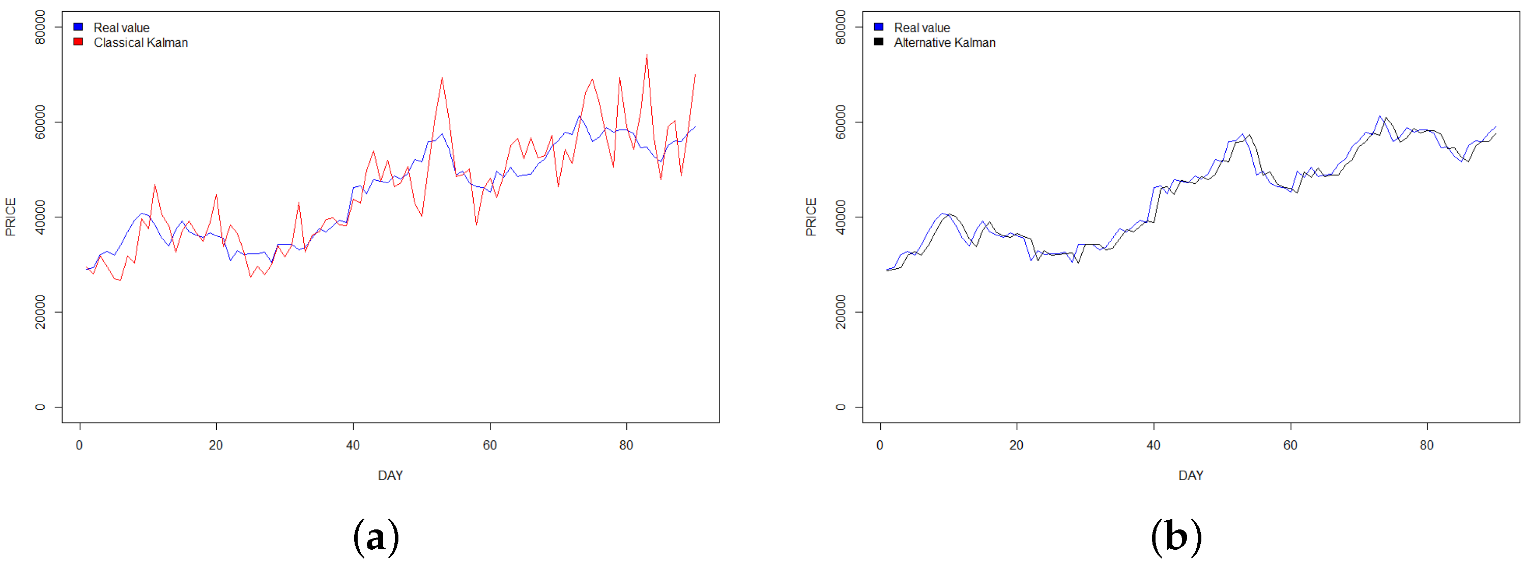
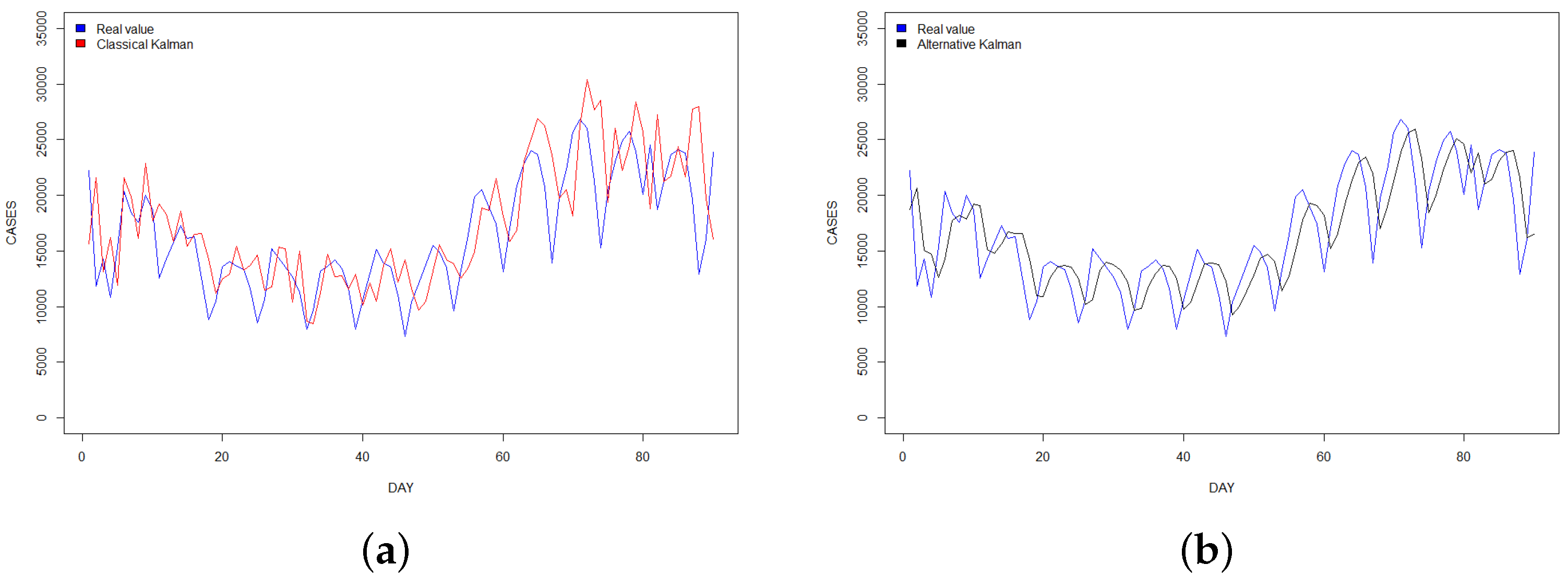
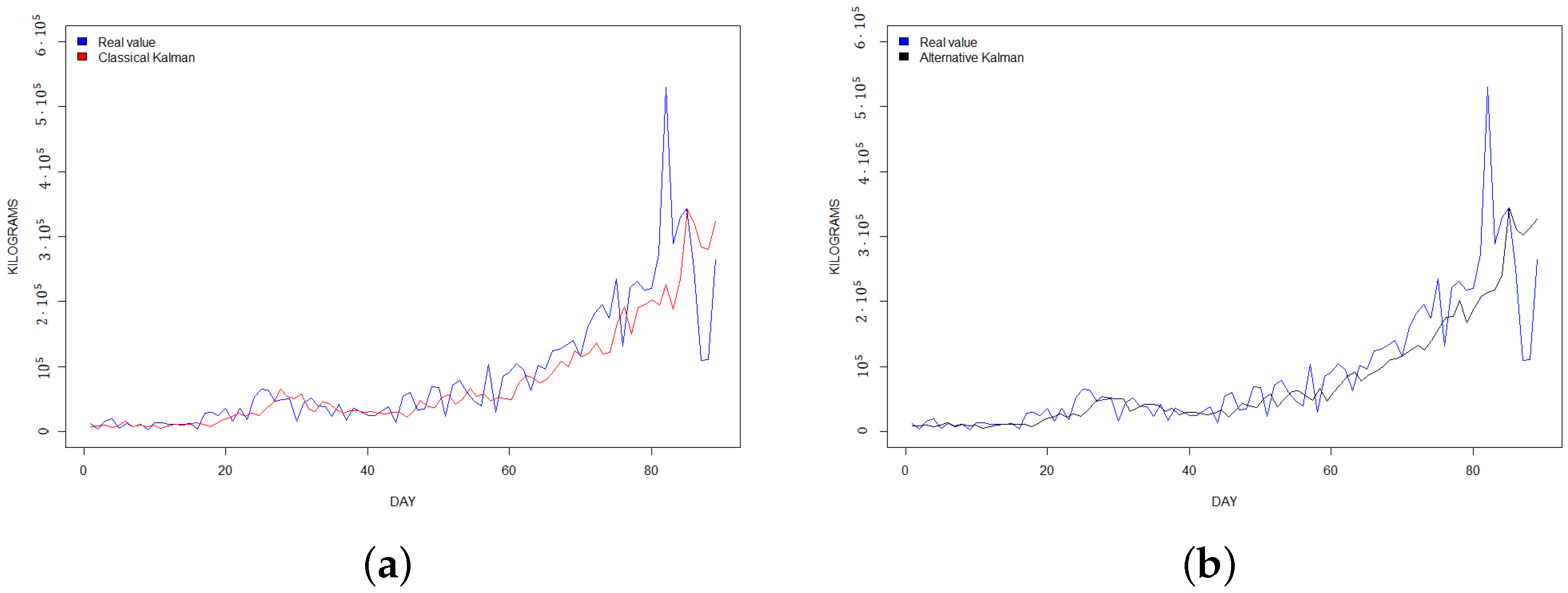
Finally, if we analyze the graphs of our predictions, we can observe that in all our study cases the alternative Kalman filter has a softer shape and contains fewer peaks than the classical Kalman filter, offering a better fit to the real values, in accord with the empirical values obtained. The graphs are shown in Figure 1, Figure 2 and Figure 3 respectively.

4. Discussion and Conclusions

The Kalman filter has traditionally been used for modeling predictive systems as a hybrid method together with the ARIMA [15,16,18] process, offering very good results. In time series where the standard deviation of the noise is large, as it happens in all the cases of our study, the Kalman filter diverges due to the simulation that must be carried out of the error as seen in the Equation (12). For high values of the standard deviation of the error, the variability that occurs in this simulation makes the method unstable. For this reason, the alternative Kalman filter developed in this work shows the best results, giving as a solution to this problem the elimination of the simulation of the error as seen in Equation (18); so we propose it as a variant of this state space anomaly for cases where the noise standard deviation is large.

The proposed model has limitations that have also been observed in research on ARIMA-based predictive systems. Firstly, our model has difficulties predicting the appearance of local maximums, so when the observations show highly variable behaviors in successive days, the model approximates more poorly than if it follows a clear increasing or decreasing trend for a longer period of time. For this reason, we appreciate that our model is better suited to Bitcoin price than the other two time series.

Another limitation of the proposed model is that it does not react very well to sudden changes in slope. If the berry yield increases very quickly in a short time period, our system detects this late, showing large errors at specific times. This problem can be observed visually in the graphs with a shift to the right of the forecasting with respect to the observed variable, which is more accentuated the greater the increase in growth. This limitation is typical of the ARIMA and ARIMA models with Kalman filter, as found in other studies [4,17,43,45]. Even more, other predictive systems based on a priori prediction show the same limitation as we can see in recent studies [46,47,48,49]. Therefore, we leave this as a limitation associated with the nature of our system that must be taken into account when using it, and we will try to solve this problem in the future with other types of models.

This work has addressed the issue of forecasting the production of fresh berries, the price of Bitcoin and the new cases of SARS-COV-2. Taking these time series, a new variant of the Kalman filter with a short-term forecast time horizon was developed, analyzed and validated.

Daily forecasts for a horizon of up to 90 days were determined by comparing the performance of the new approach with the Kalman filter. The alternative Kalman filter approach was found to be more accurate across all time series tested. The results confirm that the developed approach can be used to predict our selected time series, as well as other time series that present these same convergence problems. The search conditions associated with the standard deviation of the time series determined by the alternative Kalman filter were suggested as a generalization that improves the classical Kalman filter.

Finally, although the results of the alternative Kalman filter are similar to those obtained with the ARIMA and Naïve methods, and although it was not the aim of this work to compare the new algorithm with these simpler methods, it is important to pay attention to the type of time series data before modeling, as evidenced by the failures in SARS-COV-2 epidemic forecasting [50,51]. Among the causes of these failures, we find erroneous modeling assumptions and high sensitivity of the estimates. For example, the SARS-COV-2 pandemic death datasets (although our data refer to cases and not deaths) are fat-tailed, which makes it a mistake to use Naïve first-order methods for forecasting [51]. However, in these datasets, modeling predictive distributions rather than focusing on point estimates may be useful [50,51].

In summary, taking into account the requested limitations, we obtained a simple predictive system whose results are equal to or better than other more complex systems, thus achieving the objective of obtaining a good prediction with a simple method and information that is not sensible, and it is easy to obtain.

As the new algorithm was tested with three different time series from three different fields, the use of this algorithm can be generalized to other studies of similar conditions, such as the series presented in [23] where it would be interesting as a future line to check in what level is found with respect to the models proposed there. On the other hand, we believe that practitioners and researchers can easily improve the accuracy of their forecasts by adopting the alternative Kalman filter developed in this paper.

A final conclusion of this paper, which is often not sufficiently recognized in the literature, is that a slight variation in traditional methods is more important than it seems at first glance. For small- and medium-sized companies (SMEs), where due to the lack of large datasets, the low-quality of other independent variables or scarce computational resources, which is a real situation, accurate predictive algorithms that work without external variables and with low time consumption, are welcome.

Finally, in addition to the ARIMA models and Kalman filter, it is also recommended to compare the alternative Kalman filter approach with other types of more complex predictive models, such as ARIMAX models or neural networks, which combine different independent variables with the study variable, such as machine learning techniques [52,53,54,55,56,57,58,59].

References

- Kumar, K.A.; Spulbar, C.; Pinto, P.; Hawaldar, I.T.; Birau, R.; Joisa, J. Using Econometric Models to Manage the Price Risk of Cocoa Beans: A Case from India. Risks 2022, 10, 115. [Google Scholar] [CrossRef]
- Xu, X. Corn Cash Price Forecasting. Am. J. Agric. Econ. 2020, 102, 1297–1320. [Google Scholar] [CrossRef]
- Bórawski, P.; Bórawski, M.B.; Parzonko, A.; Wicki, L.; Rokicki, T.; Perkowska, A.; Dunn, J.W. Development of Organic Milk Production in Poland on the Background of the EU. Agriculture 2021, 11, 323. [Google Scholar] [CrossRef]
- Bo, Y.; Li, X.; Liu, K.; Wang, S.; Zhang, H.; Gao, X.; Zhang, X. Three Decades of Gross Primary Production (GPP) in China: Variations, Trends, Attributions, and Prediction Inferred from Multiple Datasets and Time Series Modeling. Remote Sens. 2022, 14, 2564. [Google Scholar] [CrossRef]
- Wang, B.; Lu, X.; Ren, Y.; Tao, S.; Gao, W. Prediction Model and Influencing Factors of CO2 Micro/Nanobubble Release Based on ARIMA-BPNN. Agriculture 2022, 12, 323. [Google Scholar] [CrossRef]
- Rathore, R.K.; Mishra, D.; Mehra, P.S.; Pal, O.; HASHIM, A.S.; Shapi’i, A.; Ciano, T.; Shutaywi, M. Real-world model for bitcoin price prediction. Inf. Process. Manag. 2022, 59, 102968. [Google Scholar] [CrossRef]
- Benvenuto, D.; Giovanetti, M.; Vassallo, L.; Angeletti, S.; Ciccozzi, M. Application of the ARIMA model on the COVID-2019 epidemic dataset. Data Brief 2020, 29, 105340. [Google Scholar] [CrossRef]
- Fliessbach, A.; Ihle, R. Cycles in cattle and hog prices in South America. Aust. J. Agric. Resour. Econ. 2020, 64, 1167–1183. [Google Scholar] [CrossRef]
- Nason, J.; Smith, G. Measuring the Slowly Evolving Trend in US Inflation with Professional Forecasts. J. Appl. Econom. 2020, 36, 1–17. [Google Scholar] [CrossRef]
- Wu, J.C.; Xia, F. Negative Interest Rate Policy and the Yield Curve. J. Appl. Econom. 2020, 35, 653–672. [Google Scholar] [CrossRef]
- Beckmann, J.; Koop, G.; Korobilis, D.; Schossler, R.A. Exchange rate predictability and dynamic Bayesian learning. J. Appl. Econom. 2020, 35, 410–421. [Google Scholar] [CrossRef]
- Seetharam, Y. Investigating the low-risk anomaly in South Africa. Rev. Behav. Financ. 2021, 14, 277–295. [Google Scholar] [CrossRef]
- Narci, R.; Delattre, M.; Larédo, C.; Vergu, E. Inference for partially observed epidemic dynamics guided by Kalman filtering techniques. Comput. Stat. Data Anal. 2021, 164, 107319. [Google Scholar] [CrossRef]
- Jutinico, A.L.; Vergara, E.; García, C.E.A.; Palencia, M.A.; non, A.D.O.C. Robust Kalman filter for Tuberculosis Incidence Time Series Forecasting. IFAC Pap. 2021, 54, 424–429. [Google Scholar] [CrossRef]
- Aamir, M.; Shabri, A. Modelling and forecasting monthly crude oil price of Pakistan: A comparative study of ARIMA, GARCH and ARIMA Kalman model. AIP Conf. Proc. 2016, 1750, 060015. [Google Scholar] [CrossRef]
- Xu, D.w.; Wang, Y.d.; Jia, L.m.; Qin, Y.; Dong, H.h. Real-time road traffic state prediction based on ARIMA and Kalman filter. Front. Inf. Technol. Electron. Eng. 2017, 18, 287–302. [Google Scholar] [CrossRef]
- Selvaraj, J.; Arunachalam, V.; Coronado-Franco, K. Time-series modeling of fishery landings in the Colombian Pacific Ocean using an ARIMA model. Reg. Stud. Mar. Sci. 2020, 39, 101477. [Google Scholar] [CrossRef]
- Muhammad, A. Using the Kalman filter with ARIMA for the COVID-19 pandemic dataset of Pakistan. Data Brief 2020, 31, 105854. [Google Scholar] [CrossRef]
- Lagos-Álvareza, B.; Padilla, L.; Mateu, J.; Ferreira, G. A Kalman filter method for estimation and prediction of space-time data with an autoregressive structure. J. Stat. Plan. Inference 2019, 203, 117–130. [Google Scholar] [CrossRef]
- Ewald, C.; Zou, Y. Analytic formulas for futures and options for a linear quadratic jump diffusion model with seasonal stochastic volatility and convenience yield: Do fish jump? Eur. J. Oper. Res. 2021, 294, 801–815. [Google Scholar] [CrossRef]
- Pedregal, D.J. New algorithms for automatic modelling and forecasting of decision support systems. Decis. Support Syst. 2021, 148, 113585. [Google Scholar] [CrossRef]
- Wai Hoh, T.; Adrian, R. Model identification for ARMA time series through convolutional neural networks. Decis. Support Syst. 2021, 146, 113544. [Google Scholar] [CrossRef]
- Makridakis, S.; Spiliotis, E.; Assimakopoulos, V. The M4 Competition: 100,000 time series and 61 forecasting methods. Int. J. Forecast. 2020, 36, 54–74. [Google Scholar] [CrossRef]
- Diebold, F.X.; Mariano, R.S. Comparing Predictive Accuracy. J. Bus. Econ. Stat. 1995, 13, 253–263. [Google Scholar] [CrossRef]
- Harvey, D.; Leybourne, S.; Newbold, P. Testing the equality of prediction mean squared errors. Int. J. Forecast. 1997, 13, 281–291. [Google Scholar] [CrossRef]
- Team, R.C. R: A Language and Environment for Statistical Computing; R Foundation for Statistical Computing: Vienna, Austria, 2013. [Google Scholar]
- Box, G.E.P.; Jenkins, G.M. Time Series Analysis: Forecasting and Control, revised ed.; Holden-Day: Cleveland, Australia, 1976. [Google Scholar]
- Hannan, E.; Rissanen, J. Recursive estimation of mixed autoregressive-moving average order. Biometrika 1982, 69, 81–94. [Google Scholar] [CrossRef]
- Monahan, J. A note on enforcing stationarity in autoregressive-moving average models. Biometrika 1984, 71, 403–404. [Google Scholar] [CrossRef]
- Harvey, A.C. Forecasting, Structural Time Series Models and the Kalman Filter; Cambridge University Press: Cambridge, UK, 1990. [Google Scholar] [CrossRef]
- Hamilton, J.D. Handbook of Econometrics. In State-Space Models, 1st ed.; Elsevier: Amsterdam, The Netherlands, 1994; Volume 4, Chapter 5; pp. 3039–3080. [Google Scholar] [CrossRef]
- Singhal, A.; Rafiuddin, A. Role of Bitcoin on Economy. Lect. Notes Eng. Comput. Sci. 2014, 2, 1028–1033. [Google Scholar]
- Seetharaman, A.; Saravanan, A.; Patwa, N.; Mehta, J. Impact of Bitcoin as a World Currency. Account. Financ. Res. 2017, 6, 230. [Google Scholar] [CrossRef]
- Holtmeier, M.; Sandner, P. The Impact of Cryptocurrencies on Developing Countries; FSBC Working Paper; Frankfurt School of Finance & Management: Frankfurt am Main, Germany, 2019. [Google Scholar]
- Yaneva, M.; The Impact of Cryptocurrencies on the Economy. CSIE Working Papers. 2020, pp. 113–118. Available online: https://csei.ase.md/wp/files/issue16/WPIssue16113-118YAN.pdf (accessed on 30 October 2021).
- Guo, H.; Zhang, D.; Liu, S.; Wang, L.; Ding, Y. Bitcoin price forecasting: A perspective of underlying blockchain transactions. Decis. Support Syst. 2021, 151, 113650. [Google Scholar] [CrossRef]
- Chen, W.; Xu, H.; Jia, L.; Gao, Y. Machine learning model for Bitcoin exchange rate prediction using economic and technology determinants. Int. J. Forecast. 2021, 37, 28–43. [Google Scholar] [CrossRef]
- Koo, E.; Kim, G. Prediction of Bitcoin price based on manipulating distribution strategy. Appl. Soft Comput. 2021, 110, 107738. [Google Scholar] [CrossRef]
- Shu, M.; Zhu, W. Real-time prediction of Bitcoin bubble crashes. Phys. A Stat. Mech. Its Appl. 2020, 548, 124477. [Google Scholar] [CrossRef]
- Saba, A.I.; Elsheikh, A.H. Forecasting the prevalence of COVID-19 outbreak in Egypt using nonlinear autoregressive artificial neural networks. Process. Saf. Environ. Prot. 2020, 141, 1–8. [Google Scholar] [CrossRef] [PubMed]
- Khan, F.M.; Gupta, R. ARIMA and NAR based prediction model for time series analysis of COVID-19 cases in India. J. Saf. Sci. Resil. 2020, 1, 12–18. [Google Scholar] [CrossRef]
- Petropoulos, F.; Makridakis, S.; Stylianou, N. COVID-19: Forecasting confirmed cases and deaths with a simple time-series model. Int. J. Forecast. 2020, 38, 439–452. [Google Scholar] [CrossRef]
- Hernandez-Matamoros, A.; Fujita, H.; Hayashi, T.; Perez-Meana, H. Forecasting of COVID19 per regions using ARIMA models and polynomial functions. Appl. Soft Comput. 2020, 96, 106610. [Google Scholar] [CrossRef]
- González-Ramírez, M.; Santoyo-Cortés, V.; Arana-Coronado, J.; Muñoz Rodríguez, M. The insertion of Mexico into the global value chain of berries. World Dev. Perspect. 2020, 20, 100240. [Google Scholar] [CrossRef]
- Yang, H.; O’Connell, J. Short-term carbon emissions forecast for aviation industry in Shanghai. J. Clean. Prod. 2020, 275, 122734. [Google Scholar] [CrossRef]
- Khiem, N.M.; Takahashi, Y.; Dong, K.T.P.; Yasuma, H.; Kimura, N. Predicting the price of Vietnamese shrimp products exported to the US market using machine learning. Soil Tillage Res. 2021, 87, 411–423. [Google Scholar] [CrossRef]
- Maldaner, L.; Corrêdo, L.; Canata, T.; Molin, J. Predicting the sugarcane yield in real-time by harvester engine parameters and machine learning approaches. Comput. Electron. Agric. 2021, 181, 105945. [Google Scholar] [CrossRef]
- Mahto, A.; Alam, M.A.; Biswas, R.; Ahmed, J.; Alam, S.I. Short-Term Forecasting of Agriculture Commodities in Context of Indian Market for Sustainable Agriculture by Using the Artificial Neural Network. J. Food Qual. 2021, 2021, 9939906. [Google Scholar] [CrossRef]
- Yin, H.; Jin, D.; Gu, Y.H.; Park, C.J.; Han, S.K.; Yoo, S.J. STL-ATTLSTM: Vegetable Price Forecasting Using STL and Attention Mechanism-Based LSTM. Agriculture 2020, 10, 2492. [Google Scholar] [CrossRef]
- Ioannidis, J.P.; Cripps, S.; Tanner, M.A. Forecasting for COVID-19 has failed. Int. J. Forecast. 2022, 38, 423–438. [Google Scholar] [CrossRef]
- Taleb, N.N.; Bar-Yam, Y.; Cirillo, P. On single point forecasts for fat-tailed variables. Int. J. Forecast. 2022, 38, 413–422. [Google Scholar] [CrossRef]
- Kongcharoen, C.; Kruangpradit, T. Autoregressive Integrated Moving Average with Explanatory Variable (ARIMAX) Model for Thailand Export. Available online: https://forecasters.org/wp-content/uploads/gravity_forms/7-2a51b93047891f1ec3608bdbd77ca58d/2013/07/Kongcharoen_Chaleampong_ISF2013.pdf (accessed on 3 July 2022).
- Yang, M.; Xie, J.; Mao, P.; Wang, C.; Ye, Z. Application of the ARIMAX Model on Forecasting Freeway Traffic Flow. In CICTP 2017: Transportation Reform and Change—Equity, Inclusiveness, Sharing, and Innovation; American Society of Civil Engineers: Reston, VA, USA, 2018; pp. 593–602. [Google Scholar]
- Wang, Q.; Li, S.; Li, R.; Ma, M. Forecasting U.S. Shale Gas Monthly Production Using a Hybrid ARIMA and Metabolic Nonlinear Grey Model. Energy 2018, 160, 378–387. [Google Scholar] [CrossRef]
- Khan, M.M.H.; Muhammad, N.S.; El-Shafie, A. Wavelet Based Hybrid ANN-ARIMA Models for Meteorological Drought Forecasting. J. Hydrol. 2020, 590, 125380. [Google Scholar] [CrossRef]
- Li, Z.; Han, J.; Song, Y. On the forecasting of high frequency financial time series based on ARIMA model improved by Deep Learning. J. Forecast. 2020, 39, 1081–1097. [Google Scholar] [CrossRef]
- Fang, Y.; Guan, B.; Wu, S.; Heravi, S. Optimal Forecast Combination Based on Ensemble Empirical Mode Decomposition for Agricultural Commodity Futures Prices. J. Forecast. 2020, 39, 877–886. [Google Scholar] [CrossRef]
- Guo, Y.; Huajian, Z.; Zhang, S.; Wang, Y.; Chow, D. Modeling and Optimization of Environment in Agricultural Greenhouses for Improving Cleaner and Sustainable Crop Production. J. Clean. Prod. 2020, 285. [Google Scholar] [CrossRef]
- Hecq, A.; Issler, J.; Telg, S. Mixed Causal? Noncausal Autoregressions with Exogenous Regressors. J. Appl. Econ. 2020, 35. [Google Scholar] [CrossRef]
Figure 1.
Bitcoin price prediction between 1 January 2021–31 March 2021. (a) Classical Kalman filter; (b) alternative Kalman filter.
Figure 2.
SARS-COV-2 cases prediction between 1 January 2021–31 March 2021. (a) Classical Kalman filter; (b) alternative Kalman filter.
Figure 3.
Berry production prediction between 1 January 2021–31 March 2021. (a) Classical Kalman filter; (b) alternative Kalman filter.