Hybrid Control Scheme for Projective Lag Synchronization of Riemann–Liouville Sense Fractional Order Memristive BAM NeuralNetworks with Mixed Delays

 , , ,
, , ,  and
and 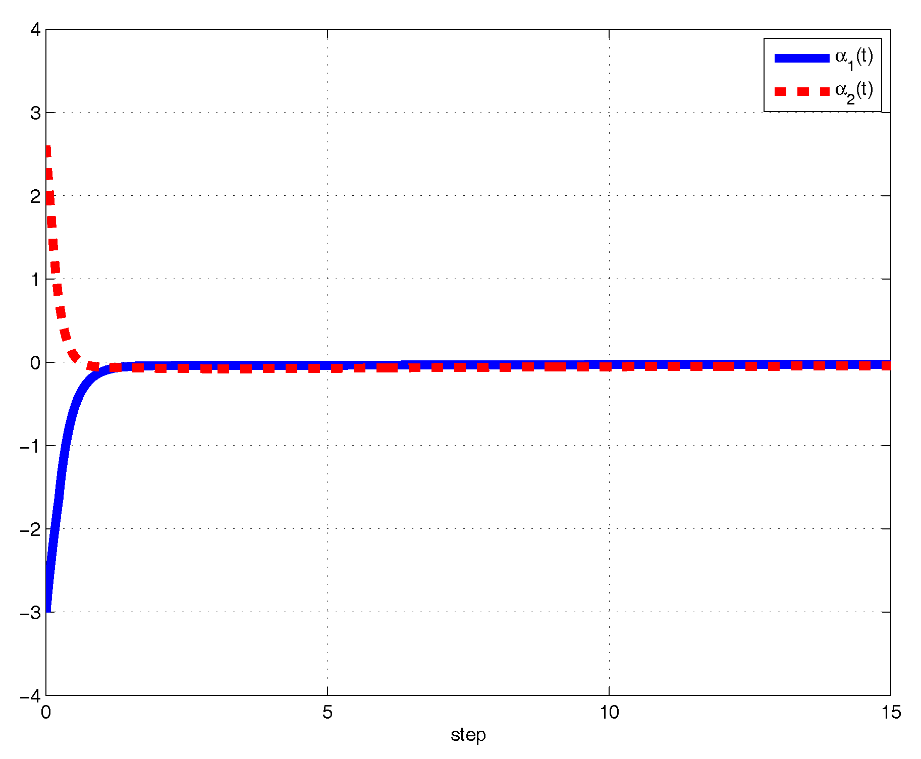
Abstract
:1. Introduction
- Based on the theory of differential inclusions and set valued map analysis, the drive-response synchronization error system is formulated.
- A novel hybrid controller, which is the combination of open loop control and adaptive state feedback control are designed to ensure the projective lag synchronization criteria for FOMBNNs with mixed time delays.
- Based on the designed hybrid controller and Barbalats lemma, the projective lag synchronization criteria for the drive-response models of the considered FOMBNNs are studied demonstrably.
- As a special case of complete synchronization, anti-synchronization and projective synchronization of FMNNs is also investigated. Hence, Corollary 3 is new and these results has not been seen in any of the literature.
- In contrast to the existing results in the literature, the hybrid control BAM type neural networks and mixed time delays have not taken into consideration; however, our proposed results make it up.
2. Preliminaries and Problem Statement
- (1)
- ;
- (2)
- ;
- (3)
- .
3. Main Results
- 1.
- Based on the hybrid control, we choose the values of and according to assumptions and system parameters.
- 2.
- Next, justify whetherWhen we adjust the above parameters of the system, then the control gains of the hybrid controller (7) can be tuned slightly to realize a projective synchronization goal.
- 3.
- Next, we choose a time lag and projective coefficient .
- 4.
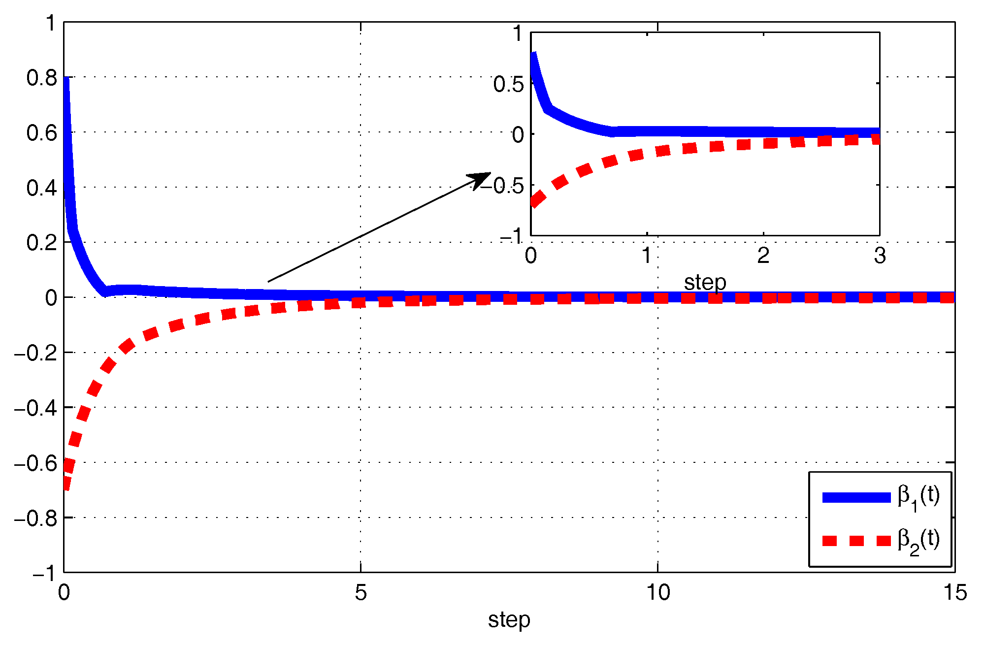
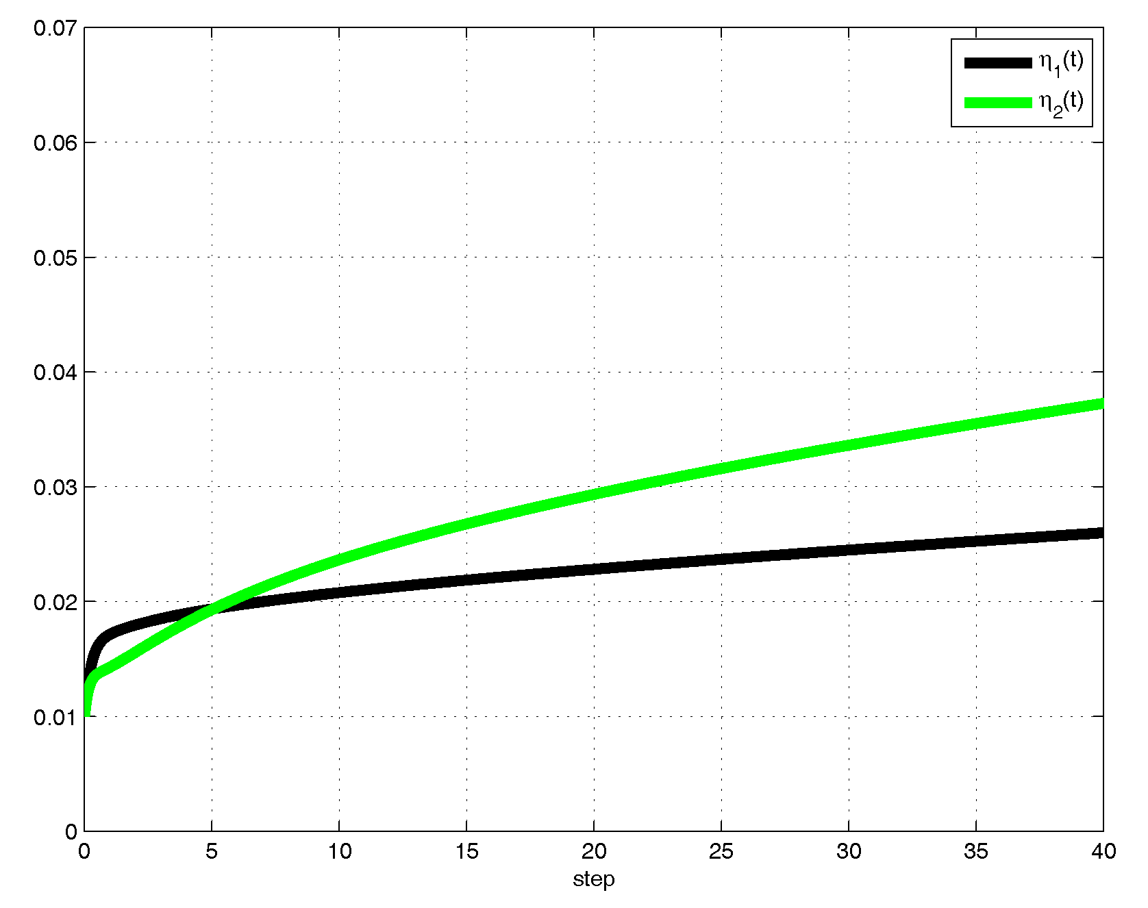
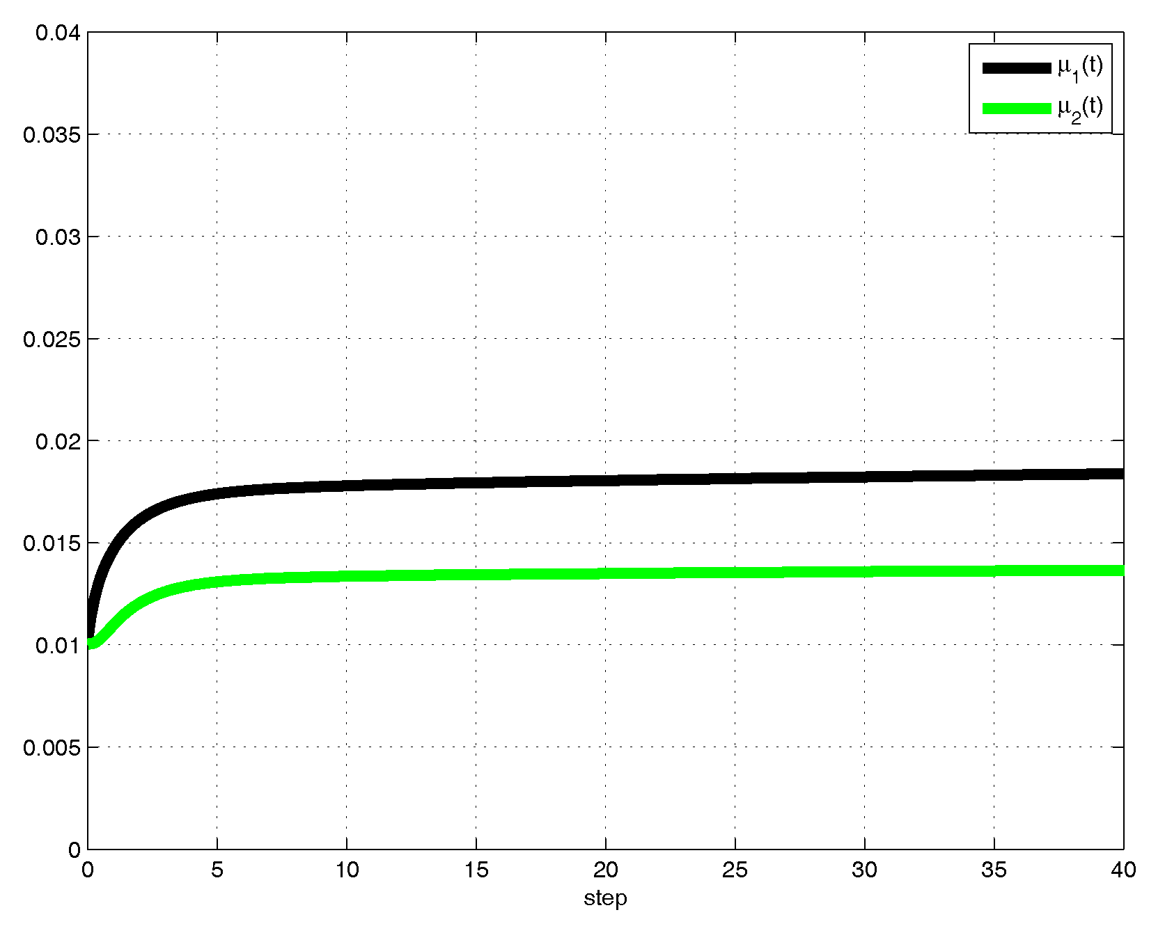
- Then, by using the dedicated simulation software tools and also selecting the simulation step size , the output trajectories confirm that the tuned control gains converge gradually to some positive constants.
4. Numerical Example
5. Conclusions
Author Contributions
Funding
Acknowledgments
Conflicts of Interest
References
- Huang, C.; Liu, B. New studies on dynamic analysis of inertial neural networks involving non-reduced order method. Neurocomputing 2019, 325, 283–287. [Google Scholar] [CrossRef]
- Wang, J.; Huang, C.; Huang, L. Discontinuity-induced limit cycles in a general planar piecewise linear system of saddle–focus type. Nonlinear Anal. Hybrid Syst. 2019, 33, 162–178. [Google Scholar] [CrossRef]
- Wang, J.; Chen, X.; Huang, L. The number and stability of limit cycles for planar piecewise linear systems of node-saddle type. J. Math. Anal. Appl. 2019, 469, 405–427. [Google Scholar] [CrossRef]
- Chen, T.; Huang, L.; Yu, P.; Huang, W. Bifurcation of limit cycles at infinity in piecewise polynomial systems. Nonlinear Anal. Real World Appl. 2018, 41, 82–106. [Google Scholar] [CrossRef]
- Cai, Z.; Huang, J.; Huang, L. Periodic orbit analysis for the delayed Filippov system. Proc. Am. Math. Soc. 2018, 146, 4667–4682. [Google Scholar] [CrossRef]
- Yang, C.; Huang, L.; Li, F. Exponential synchronization control of discontinuous nonautonomous networks and autonomous coupled networks. Complexity 2018, 2018, 6164786. [Google Scholar] [CrossRef]
- Zuo, Y.; Wang, Y.; Liu, X. Adaptive robust control strategy for rhombus-type lunar exploration wheeled mobile robot using wavelet transform and probabilistic neural network. Comput. Appl. Math. 2018, 37, 314–337. [Google Scholar] [CrossRef]
- Hu, H.; Zou, X. Existence of an extinction wave in the fisher equation with a shifting habitat. Proc. Am. Math. Soc. 2017, 145, 4763–4771. [Google Scholar] [CrossRef]
- Song, C.; Fei, S.; Cao, J.; Huang, C. Robust Synchronization of Fractional-Order Uncertain Chaotic Systems Based on Output Feedback Sliding Mode Control. Mathematics 2019, 7, 599. [Google Scholar] [CrossRef]
- Cai, Z.; Huang, J.; Huang, L. Generalized Lyapunov-Razumikhin method for retarded differential inclusions: Applications to discontinuous neural networks. Discret. Contin. Dyn. Syst. Ser. B 2017, 22, 3591–3614. [Google Scholar] [CrossRef] [Green Version]
- Tan, Y.; Zhang, M. Global exponential stability of periodic solutions in a nonsmooth model of hematopoiesis with time-varying delays. Math. Methods Appl. Sci. 2017, 40, 5986–5995. [Google Scholar] [CrossRef]
- Huang, C.; Cao, J.; Wen, F.; Yang, X. Stability Analysis of SIR Model with Distributed Delay on Complex Networks. PLoS ONE 2016, 11, e0158813. [Google Scholar] [CrossRef] [PubMed]
- Diethelm, K. The Analysis of Fractional Differential Equations; Springer: Berlin, Germany, 2010. [Google Scholar]
- Hilfer, R. Applications of Fractional Calculus in Physics; World Scientific: Singapore, 2000; Volume 128. [Google Scholar]
- Kilbas, A.; Srivastava, A.; Trujillo, J.J. Theory and Applications of Fractional Differential Equations; Elsevier Science Limited: Amsterdam, The Netherlands, 2006; Volume 204. [Google Scholar]
- Podlubny, I. Fractional Differential Equations; Academic Press: San Diego, CA, USA, 1999. [Google Scholar]
- Laskin, N. Fractional market dynamics. Phys. A Stat. Mech. Appl. 2000, 287, 482–492. [Google Scholar] [CrossRef]
- Lundstrom, B.N.; Higgs, M.H.; Spain, W.J.; Fairhall, A.L. Fractional differentiation by neocortical pyramidal neurons. Nat. Neurosci. 2008, 11, 1335–1342. [Google Scholar] [CrossRef] [PubMed]
- Petras, I. Fractional-Order Nonlinear Systems: Modeling, Analysis and Simulation; Springer: Berlin, Germany, 2011. [Google Scholar]
- Ali, S.; Narayanan, G.; Sevgen, S.; Sheher, V.; Arik, S. Global stability analysis of fractional-order fuzzy BAM neural networks with time delay and impulsive effects. Commun. Nonlinear Sci. Numer. Simul. 2019, 78, 104853. [Google Scholar]
- Wang, F.; Yang, Y.; Xu, X.; Li, L. Global asymptotic stability of impulsive fractional-order BAM neural networks with time delay. Neural Comput. Appl. 2017, 28, 345–352. [Google Scholar] [CrossRef]
- Wu, A.; Zeng, Z.; Song Global, S. Mittag–Leffler stabilization of fractionalorder bidirectional associative memory neural networks. Neurocomputing 2016, 177, 489–496. [Google Scholar] [CrossRef]
- Ye, R.; Liu, X.; Zhang, H.; Cao, J. Global Mittag–Leffler synchronization for fractional-order BAM neural networks with impulses and multiple variable delays via delayed-feedback control strategy. Neural Process. Lett. 2019, 49, 1–18. [Google Scholar] [CrossRef]
- Rajivganthi, C.; Rihan, F.; Laxshmanan, S.; Rakkiappan, R.; Muthuumar, P. Synchronization of memristor-based delayed BAM neural networks with fractional-order derivatives. Complexity 2016, 21, 412–426. [Google Scholar] [CrossRef]
- Duan, L.; Fang, X.; Huang, C. Global exponential convergence in a delayed almost periodic Nicholson’s blowflies model with discontinuous harvesting. Math. Methods Appl. Sci. 2018, 41, 1954–1965. [Google Scholar] [CrossRef]
- Huang, C.; Liu, B.; Tian, X.; Yang, L.; Zhang, X. Global convergence on asymptotically almost periodic SICNNs with nonlinear decay functions. Neural Process. Lett. 2019, 49, 625–641. [Google Scholar] [CrossRef]
- Huang, C.; Zhang, H.; Huang, L. Almost periodicity analysis for a delayed Nicholson’s blowflies model with nonlinear density-dependent mortality term. Commun. Pure Appl. Anal. 2019, 18, 3337–3349. [Google Scholar] [CrossRef]
- Yang, X.; Zhu, Q.; Huang, C. Generalized lag-synchronization of chaotic mix-delayed systems with uncertain parameters and unknown perturbations. Nonlinear Anal. Real World Appl. 2011, 12, 93–105. [Google Scholar] [CrossRef]
- Huang, C.; Qiao, Y.; Huang, L. Agarwal, Dynamical behaviors of a food-chain model with stage structure and time delays. Adv. Differ. Equ. 2018, 2018, 186. [Google Scholar] [CrossRef]
- Huang, C.; Zhang, H. Periodicity of non-autonomous inertial neural networks involving proportional delays and non-reduced order method. Int. J. Biomath. 2019, 12, 1950016. [Google Scholar] [CrossRef]
- Zhu, Q.; Huang, C.; Yang, X. Exponential stability for stochastic jumping BAM neural networks with time-varying and distributed delays. Nonlinear Anal. Hybrid Syst. 2011, 5, 52–77. [Google Scholar] [CrossRef]
- Huang, C.; Su, R.; Cao, J.; Xiao, S. Asymptotically stable high-order neutral cellular neural networks with proportional delays and D operators. Math. Comput. Simul. 2019. [Google Scholar] [CrossRef]
- Huang, C.; Zhang, H.; Cao, J.; Hu, H. Stability and Hopf bifurcation of a delayed prey-predator model with disease in the predator. Int. J. Bifurc. Chaos 2019, 29, 1950091. [Google Scholar] [CrossRef]
- Huang, C.; Yang, Z.; Yi, T.; Zou, X. On the basins of attraction for a class of delay differential equations with non-monotone bistable nonlinearities. J. Differ. Equ. 2014, 256, 2101–2114. [Google Scholar] [CrossRef]
- Wu, H.; Zhang, X.; Xue, S.; Niu, P. Quasi-uniform stability of Caputo-type fractional-order neural networks with mixed delay. Int. J. Mach. Learn. Cybern. 2017, 8, 1501–1511. [Google Scholar] [CrossRef]
- Zhang, H.; Ye, R.; Cao, J.; Alsaedi, A. Existence and globally asymptotic stability of equilibrium solution for fractional-order hybrid BAM neural networks with distributed delays and impulses. Complexity 2017, 2017, 6875874. [Google Scholar] [CrossRef]
- Chua, L.Q. Memristor-the missing circuit element. IEEE Trans. Circuit Theory 1971, 18, 507–519. [Google Scholar] [CrossRef]
- Strukov, D.; Snider, G.; Stewart, D.; Williams, R. The missing memristor found. Nature 2008, 453, 80–83. [Google Scholar] [CrossRef]
- Kim, H.; Sah, M.P.; Yang, C.; Roska, T.; Chua, L.O. Memristor bridge synapses. Proc. IEEE 2012, 100, 2061–2070. [Google Scholar] [CrossRef]
- Bao, H.B.; Cao, J.; Kurths, J. State estimation of fractional-order delayed memristive neural networks. Nonlinear Dyn. 2018, 2, 1215–1225. [Google Scholar] [CrossRef]
- Chang, W.; Zhu, S.; Li, J.; Sun, K. Global Mittag–Leffler stabilization of fractional-order complex-valued memristive neural networks. Appl. Math. Comput. 2018, 338, 346–362. [Google Scholar] [CrossRef]
- Wu, A.; Zeng, Z. Global Mittag–Leffler stabilization of fractional-Order memristive neural networks. IEEE Trans. Neural Netw. Learn. Syst. 2017, 28, 206–217. [Google Scholar] [CrossRef]
- Li, X.; Fang, J.A.; Zhang, W.; Li, H. Finite-time synchronization of fractional-order memristive recurrent neural networks with discontinuous activation functions. Neurocomputing 2018, 316, 284–293. [Google Scholar] [CrossRef]
- Pecora, L.; Carrol, T. Synchronization in chaotic systems. Phys. Rev. Lett. 1990, 64, 821–824. [Google Scholar] [CrossRef]
- Liu, X.; Jiang, N.; Cao, J. Finite-time stochastic stabilization for BAM neural networks with uncertainties. J. Frankl. Inst. 2013, 350, 2109–2123. [Google Scholar] [CrossRef]
- Abdurahman, A.; Jiang, H.; Teng, Z. Exponential lag synchronization for memristor-based neural networks with mixed time delays via hybrid switching control. J. Frankl. Inst. 2016, 353, 2859–2880. [Google Scholar] [CrossRef]
- Velmurugan, G.; Rakkiyappan, R. Hybrid projective synchronization of fractional-order memristor-based neural networks with time delays. Nonlinear Dyn. 2016, 83, 419–432. [Google Scholar] [CrossRef]
- Wu, H.; Wang, L.; Niu, P.; Wang, Y. Global projective synchronization in finite time of nonidentical fractional order neural networks based on sliding mode control strategy. Neurocomputing 2017, 235, 264–273. [Google Scholar] [CrossRef]
- Xiao, J.; Zhong, S.; Li, Y.; Xu, F. Finite-time Mittag–Leffler synchronization of fractional-order memristive BAM neural networks with time delays. Neurocomputing 2016, 219, 431–439. [Google Scholar] [CrossRef]
- Zhang, L.; Yang, Y.; Wang, F. Lag synchronization for fractional-order memristive neural networks via period intermittent control. Nonlinear Dyn. 2017, 89, 367–381. [Google Scholar] [CrossRef]
- Popov, V. Hyperstability of Control Systems; Springer: Berlin, Germany, 1973. [Google Scholar]
- Filippov, A.F. Differential Equations with Discontinuous Right-Hand Sides; Kluwer: Dordrecht, The Netherlands, 1988. [Google Scholar]
- Henderson, J.; Ouahab, A. Fractional functional differential inclusions with finite delay. Nonlinear Anal. Theory Methods Appl. 2009, 70, 2091–2105. [Google Scholar] [CrossRef]
- Li, N.; Cao, J.D. Lag synchronization of memristor-based coupled neural networks via ω-measure. IEEE Trans. Neural Netw. Learn. Syst. 2016, 27, 686–697. [Google Scholar] [CrossRef]
- Ding, S.B.; Wang, Z.S. Lag quasi-synchronization for memristive neural networks with switching jumps mismatch. Neural Comput. Appl. 2017, 28, 4011–4022. [Google Scholar] [CrossRef]
- Bao, H.B.; Cao, J. Projective synchronization of fractional-order memristor-based neural networks. Neural Netw. 2015, 63, 1–9. [Google Scholar] [CrossRef]
- Yu, J.; Hu, C.; Jiang, H.; Fan, X. Projective synchronization for fractional neural networks. Neural Netw. 2014, 49, 87–95. [Google Scholar] [CrossRef]


© 2019 by the authors. Licensee MDPI, Basel, Switzerland. This article is an open access article distributed under the terms and conditions of the Creative Commons Attribution (CC BY) license (http://creativecommons.org/licenses/by/4.0/).
Share and Cite
Rajchakit, G.; Pratap, A.; Raja, R.; Cao, J.; Alzabut, J.; Huang, C. Hybrid Control Scheme for Projective Lag Synchronization of Riemann–Liouville Sense Fractional Order Memristive BAM NeuralNetworks with Mixed Delays. Mathematics 2019, 7, 759. https://0-doi-org.brum.beds.ac.uk/10.3390/math7080759
Rajchakit G, Pratap A, Raja R, Cao J, Alzabut J, Huang C. Hybrid Control Scheme for Projective Lag Synchronization of Riemann–Liouville Sense Fractional Order Memristive BAM NeuralNetworks with Mixed Delays. Mathematics. 2019; 7(8):759. https://0-doi-org.brum.beds.ac.uk/10.3390/math7080759
Chicago/Turabian StyleRajchakit, Grienggrai, Anbalagan Pratap, Ramachandran Raja, Jinde Cao, Jehad Alzabut, and Chuangxia Huang. 2019. "Hybrid Control Scheme for Projective Lag Synchronization of Riemann–Liouville Sense Fractional Order Memristive BAM NeuralNetworks with Mixed Delays" Mathematics 7, no. 8: 759. https://0-doi-org.brum.beds.ac.uk/10.3390/math7080759