Article

Chaotic Synchronization Using a Self-Evolving Recurrent Interval Type-2 Petri Cerebellar Model Articulation Controller †

1
Faculty of Mechanical and Aerospace, Sejong University, Seoul 143-747(05006), Korea
2
Department of Electrical Electronic and Mechanical Engineering, Lac Hong University, Bien Hoa 810000, Vietnam
3
Department of Electrical Engineering, Yuan Ze University, Taoyuan 32003, Taiwan
*
Author to whom correspondence should be addressed.
This paper is an extended version of our paper published in 2019 IEEE International Conference on System Science and Engineering (ICSSE 2019), Dong Hoi, Vietnam, 20–21 July 2019; pp. 420–424.
Submission received: 2 December 2019 / Revised: 11 January 2020 / Accepted: 5 February 2020 / Published: 9 February 2020
(This article belongs to the Section Fuzzy Sets, Systems and Decision Making)

Abstract

:
In this manuscript, the synchronization of four-dimensional (4D) chaotic systems with uncertain parameters using a self-evolving recurrent interval type-2 Petri cerebellar model articulation controller is studied. The design of the synchronization control system is comprised of a recurrent interval type-2 Petri cerebellar model articulation controller and a fuzzy compensation controller. The proposed network structure can automatically generate new rules or delete unnecessary rules based on the self-evolving algorithm. Furthermore, the gradient-descent method is applied to adjust the proposed network parameters. Through Lyapunov stability analysis, bounded system stability is guaranteed. Finally, the effectiveness of the proposed controller is illustrated using numerical simulations of 4D chaotic systems.

1. Introduction

Recently, chaotic synchronization has attracted academic attention due to its nonlinear phenomena characteristic. Recent studies have demonstrated that chaotic synchronization can be applied to various disciplines, such as economics and chemistry as well as mechanical systems, information systems, and electronic and communication systems [1]. In recent years, a number of real-life applications have been studied by [2,3,4,5,6]. In 2016, Naderi and Kheiri proposed a secure-communication method using the exponential synchronization of a chaotic system [2]. In 2017, Pappu et al. presented an electronic implementation of Lorenz chaotic-oscillator synchronization for bistatic-radar applications [3]. In 2019, Jayaprasath et al. introduced secure optical communication using chaotic semiconductor lasers [4]. In addition, in 2019, Mandal and Das established chaos-based color image encryption using microcontrollers [5]. In recent decades, various control methods have been reported to synchronize master-slave chaotic systems, such as adaptive control [7], fuzzy control [8], fuzzy-brain emotional-learning networks [9], sliding-mode control [10], and cerebellar model articulation control [11]. However, the majority of these methods are complex, and the controlling performance requires improvement.
The cerebellar model articulation controller (CMAC) is a type of neural network based on a model of the mammalian cerebellum (associative memory), which was proposed by Albus [12]. Compared with other neural networks, CMAC is advantageous insofar that it has fast learning properties, simple computations, and good generalization capabilities [13]. In the past decade, CMAC has been applied to various fields, such as control systems [14,15,16,17], classification systems [18,19,20], signal processing [21,22,23], and image processing [24,25]. Due to the work of Zadeh [26], fuzzy modeling and fuzzy control have attracted many researchers since said methods can be used to convert problems into simple human terms. The recent progress of fuzzy-control systems has eventuated in many novel results [27,28,29,30,31,32,33]. Similar to the type-1 fuzzy system, the CMAC with type-1 membership functions (T1MFs) cannot effectively deal with the uncertainty associated with system internalities and externalities [34]. To address these uncertainties, type-2 membership functions (T2MFs) were introduced by Zadel [35]. Recent studies have proven the superior effectiveness of T2MFs over T1MFs [36,37,38]. To reduce the computational complexity of type-2 fuzzy logic systems (T2FLS), interval type-2 fuzzy logic systems (IT2FLS) were established in 2000 by Liang and Mendel [39]. Recently, by combining the advantages of CMAC and IT2FLS, the interval type-2 fuzzy CMAC (IT2CMAC) was developed and applied to various fields [40,41,42,43].
Due to the work of Peterson and Looney [44,45], Petri nets (PNs) and fuzzy PNs (FPNs) have been widely investigated in various fields [46,47,48,49,50]. A PN is a directed, weighted, and bipartite graph in which each node is either a place or a transition. The transition nodes are enabled when the value of the inputs connected to a transition that is greater than, or equal to, the threshold value [51]. In 2019, Rosdi et al. proposed the speech intelligibility detection of children using an FPN-based classification method [46]. In 2018, Zhu et al. presented model-based fault identification using PNs [47]. In 2018, Hansen et al. introduced a FPN for soccer-ball recognition and distance prediction [50]. As a special kind of PN, FPNs have some advantages, such as simple in computation, intuitive and easy to understand [46].
The recurrent neural network (RNN) is a special kind of neural network that naturally comprises feedback connections used as internal memories [52]. Many studies have used RNNs in their control network design [53,54,55,56,57] due to their advantages of simple architecture and dynamic characteristics. In 2018, Yen et al. proposed robust adaptive sliding-mode control using recurrent fuzzy wavelet neural networks [54]. In 2016, Lin et al. introduced a piezo-flexural nanopositioning stage using a RNN and intelligent integral backstepping sliding-mode control [55]. In 2016, Sharma et al. presented a robotic manipulator using a RNN and an adaptive controller similar to proportional–integral–derivative controllers [56]. In 2016, Wang et al. proposed a switched-reluctance motor-drive system using adaptive recurrent CMAC [57].
To improve the work of [58], this paper incorporates the advantages of CMAC, IT2FLS, RNN, and FPNs to propose a recurrent interval type-2 Petri cerebellar model articulation controller (RIT2PC). However, similar to other neural networks, it is difficult to determine a suitable network size for the RIT2PC to achieve the desired performance. The majority of studies used the trial-and-error approach to obtain network size, but this method is not time-effective, and its performance requires improvement. In the past, studies have provided self-organizing and self-evolving algorithms to construct network structures autonomously [59,60,61,62,63,64,65]. In 2017, Lin et al. introduced a self-evolving function-link interval type-2 fuzzy neural network for nonlinear system identification and control [60]. In addition, in 2017, Rong et al. proposed a self-evolving fuzzy model controller for hypersonic vehicles [63]. In 2018, Ge and Zeng provided a self-evolving fuzzy system that can independently learn dynamic threshold parameters [64]. Besides being able to automatically construct networks to achieve optimal structure, the self-evolving algorithm also has disadvantages; for instance, choosing the threshold to generate and delete rules significantly affects system performance [65]. This study applies a self-evolving algorithm to establish the RIT2PC structure. Thus, the proposed controller has the advantages of the aforementioned networks, but it has a better control performance. The main contributions of this study include the following: successful development of a self-evolving RIT2PC (SRIT2PC) control system; the online learning-parameter adaptation laws are obtained using the gradient-descent method; the Lyapunov stability function is used to prove the stability of the proposed synchronization system; the effectiveness of the proposed control method is illustrated using numerical experiments of four-dimensional (4D) chaotic systems.
This study is organized as follows: system description is given in Section 2; the architecture of the proposed SRIT2PC is provided in Section 3; the illustrative examples are given in Section 4; finally, conclusions are drawn in Section 5.

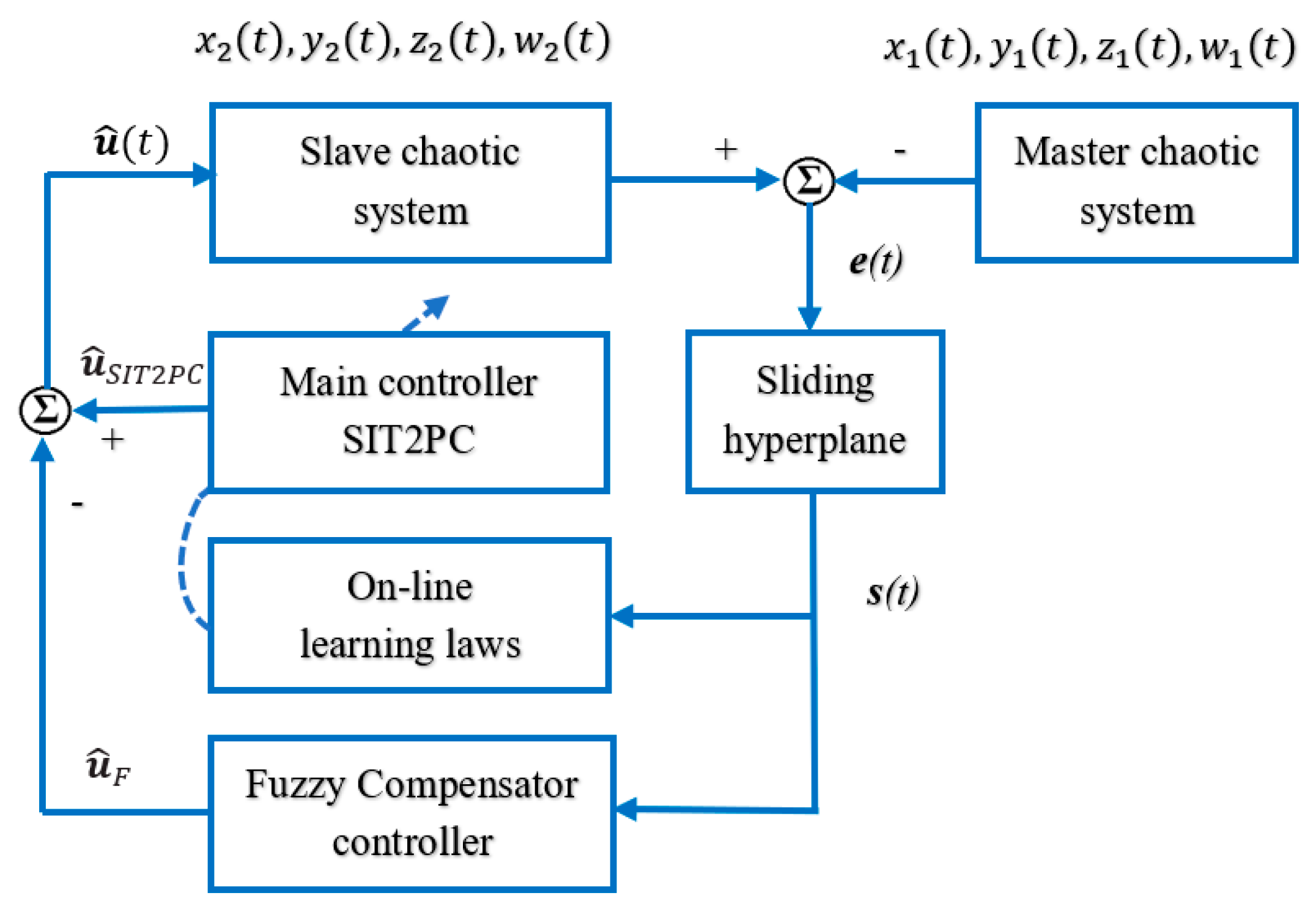
2. System Description

Consider the 4D Lorenz–Stenflo chaotic system, which was provided by Stenflo [66] as follows:
x ˙ 1 ( t ) = α ( y 1 ( t ) x 1 ( t ) ) + γ w 1 y ˙ 1 ( t ) = τ x 1 ( t ) x 1 ( t ) z 1 ( t ) λ y 1 ( t ) z ˙ 1 ( t ) = x 1 ( t ) y 1 ( t ) φ z 1 ( t ) w ˙ 1 ( t ) = x 1 ( t ) α w 1
where x 1 , y 1 , z 1 , and w 1 are the master chaotic state variables; α , τ , λ , φ , and γ are the parameters for defining the chaotic attractor:
α = ( 25 θ + 1 ) τ = ( 26 35 θ ) λ = ( 1 29 θ ) φ = ( 2.1 + θ 3 ) γ = ( θ + 1.5 )
where θ used to define the feature of the chaotic system.
When the system uncertainties, external disturbances, and control inputs are under consideration, Equation (1) can be rewritten as
x ˙ 2 ( t ) = α ( y 2 ( t ) x 2 ( t ) ) + γ w 2 + d x ( t ) + Δ f ( x 2 ) + u x ( t ) y ˙ 2 ( t ) = τ x 2 ( t ) x 2 ( t ) z 2 ( t ) λ y 2 ( t ) + d y ( t ) + Δ f ( y 2 ) + u y ( t ) z ˙ 2 ( t ) = x 2 ( t ) y 2 ( t ) φ z 2 ( t ) + d z ( t ) + Δ f ( z 2 ) + u z ( t ) w ˙ 2 ( t ) = x 2 ( t ) α w 2 + d w ( t ) + Δ f ( w 2 ) + u w ( t )
where, x 2 , y 2 , z 2 , and w 2 are the slave chaotic state variables; d x ( t ) , d y ( t ) , d z ( t ) , and d w ( t ) denote the external disturbances; Δ f ( x 2 ) , Δ f ( y 2 ) , Δ f ( z 2 ) , and Δ f ( w 2 ) denote the system uncertainties; u x ( t ) , u y ( t ) , u z ( t ) , and u w ( t ) denote the active control functions. The goal of the control system is to generate the control signal, which can force the slave system, represented by Equation (3), to synchronize with the master system, represented by Equation (1).
The tracking errors of synchronization between Equations (1) and (3) can be defined as
e x ( t ) = x 2 ( t ) x 1 ( t ) e y ( t ) = y 2 ( t ) y 1 ( t ) e z ( t ) = z 2 ( t ) z 1 ( t ) e w ( t ) = w 2 ( t ) w 1 ( t )
Thus, subtracting Equation (3) from Equation (1), yields
e ˙ x ( t ) = α ( e y ( t ) e x ( t ) ) + γ e w + d x ( t ) + Δ f ( x 2 ) + u x ( t ) e ˙ y ( t ) = τ e x ( t ) λ e y ( t ) x 2 ( t ) z 2 ( t ) + x 1 ( t ) z 1 ( t ) + d y ( t ) + Δ f ( y 2 ) + u y ( t ) e ˙ z ( t ) = x 2 ( t ) y 2 ( t ) x 1 ( t ) y 1 ( t ) φ e z ( t ) + d z ( t ) + Δ f ( z 2 ) + u z ( t ) e ˙ w ( t ) = e x ( t ) α e w ( t ) + d w ( t ) + Δ f ( w 2 ) + u w ( t )
Equation (5) can be rewritten as
e ˙ ( t ) = A e ( t ) + d ( t ) + Δ f ( t ) + u ( t )
where e ( t ) = [ e x ( t ) , e y ( t ) , e z ( t ) , e w ( t ) ] T ; A = [ α α 0 γ ( τ z 1 ( t ) ) 1 x 2 ( t ) 0 y 1 ( t ) x 2 ( t ) φ 0 1 0 0 α ]
If the system dynamics and the external disturbance can be obtained, the design of the ideal controller can be given by
u * ( t ) = A e ( t ) K e ( t ) d ( t ) Δ f ( t )
where e ˙ ( t ) = K e ( t ) and K = d i a g ( k 1 , k 2 , k 3 , k 4 ) is the feedback gain vector.
If K is selected to correspond to the coefficients of the Hurwitz polynomial, then lim t e ( t ) 0 . However, the ideal controller, which is represented by Equation (7), is generally unobtainable because the external disturbance and system dynamics cannot be precisely known in practical applications. Therefore, in this paper, an SRIT2PC is proposed to achieve the desired synchronization performance.

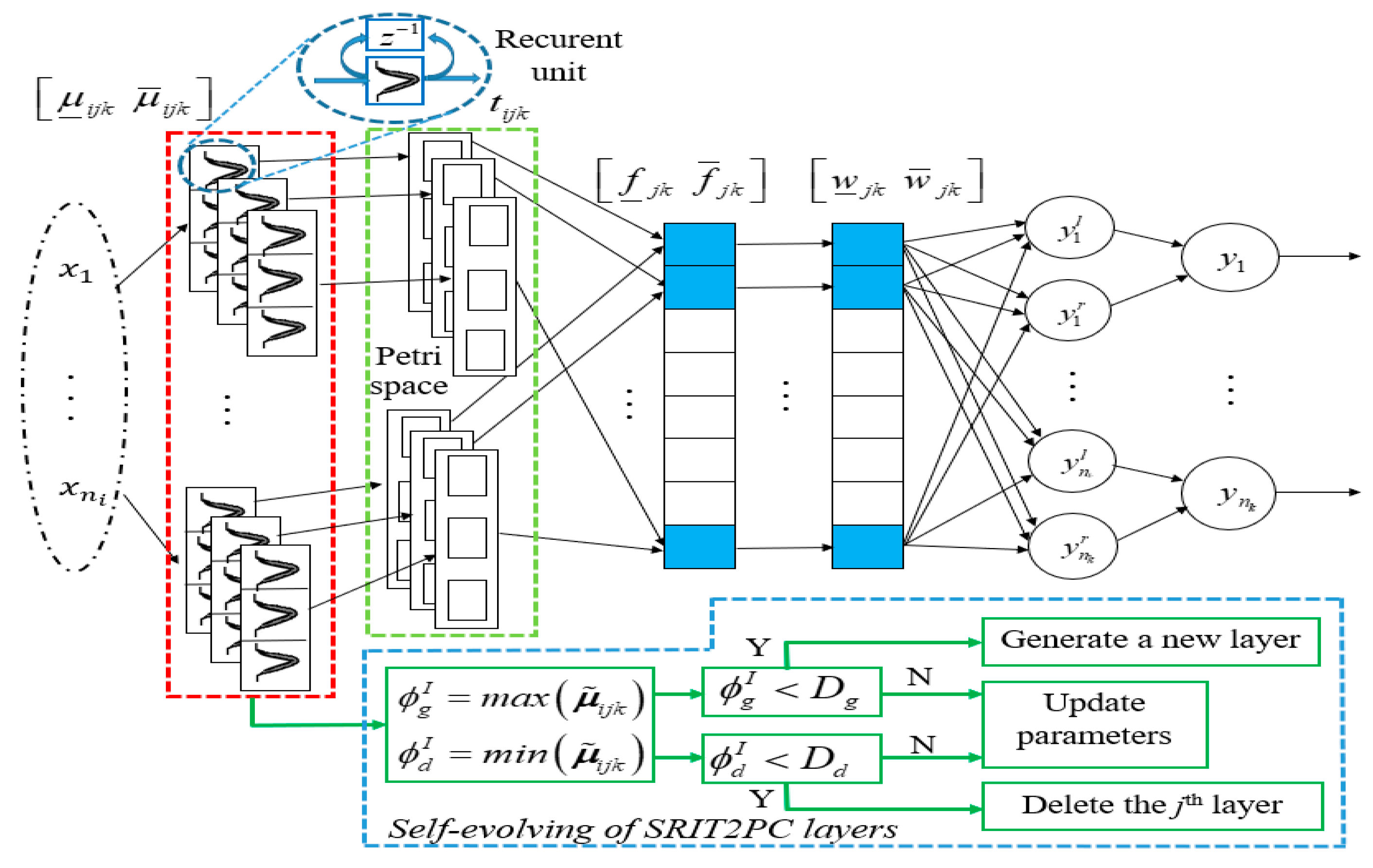
3. Architecture of SRIT2PC

The control scheme of the proposed SRIT2PC for the chaotic synchronization system is shown in Figure 1. It consists of an SRIT2PC main controller and a fuzzy compensation controller. The high-order sliding surface is applied to guarantee system stability and to achieve satisfactory control performance.

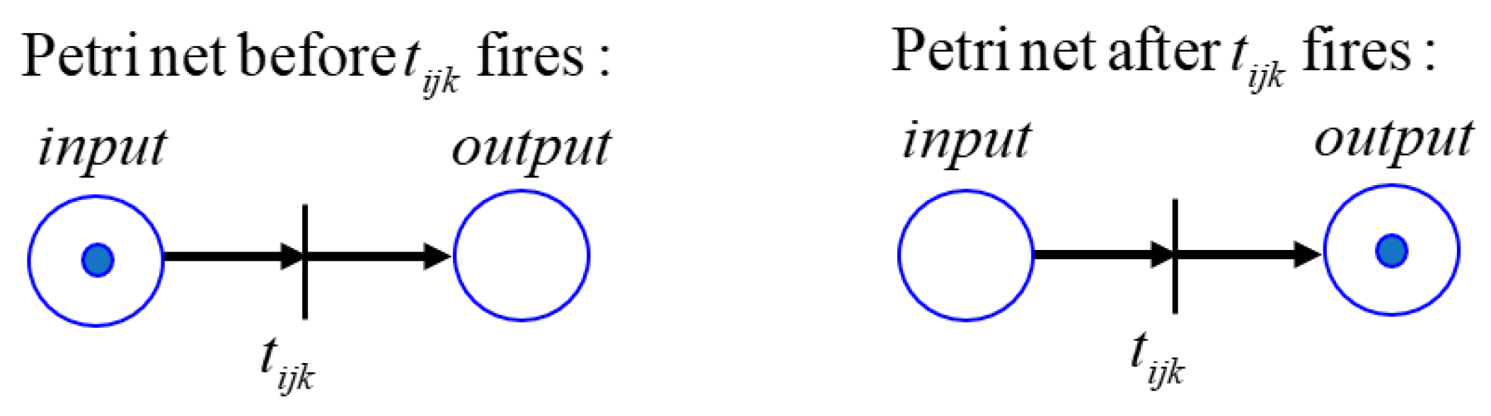
3.1. Recurrent Interval Type-2 Petri CMAC

The fuzzy inference rules of the novel SRIT2PC are given as
R u l e   λ : I F x 1 i s μ ˜ 1 j k a n d x 2 i s μ ˜ 2 j k , , a n d x n i i s μ ˜ n i j k T h e n w ˜ j k = [ w ¯ j k w ¯ j k ] f o r i = 1 , 2 , , n i ; j = 1 , 2 , , n j ; k = 1 , 2 , , n k ; λ = 1 , 2 , , n λ ;
where n i , n j and n k denote the input dimension, the number of layers, and the number of blocks in each layer, respectively; n λ denotes the total number of fuzzy rules, which is given by n λ = n j n k ; μ ˜ i j k denotes the input membership function; w ˜ j k denotes the output weight in the consequent part.
The architecture of the SRIT2PC is composed of seven spaces, shown in Figure 2. The operation in each space is outlined below.
(1). Input space: The input signal is given as X = [ x i , x i , x i , , x i ] T ϵ   n i . Herein, each input state variable, x i , is directly propagated to the association memory space.
(2). Association memory space: Several elements can be accumulated as a block, with each block performing a type-2 Gaussian membership function (T2GMF). Applying the x i signal from the input space into the T2GMF, the membership grade can be given as
μ ¯ i j k = exp { ( I ¯ r i m i j k ) 2 2 σ ¯ i j k 2 } ;   μ ¯ i j k = exp { ( I ¯ r i m i j k ) 2 2 σ ¯ i j k 2 }
I ¯ r i ( t ) = x i ( t ) + r i j k μ ¯ i j k ( t 1 ) ;   I ¯ r i ( t ) = x i ( t ) + r i j k μ ¯ i j k ( t 1 )
where μ ¯ i j k and μ ¯ i j k denote the lower and upper membership functions (MFs), respectively; the mean of the T2GMF is denoted by m i j k ; σ ¯ i j k and σ ¯ i j k denote the lower and upper variance, respectively; I ¯ r i and I ¯ r i denote the lower and upper recurrent inputs, respectively.
(3). Petri space: Each node acts as a transition operation to produce the tokens, which are then used to select suitable fuzzy laws. This can be described as
t i j k = { 1 , μ i j k g t h 0 , μ i j k < g t h
where t i j k denotes the transition nodes; μ i j k denotes the average value of μ ¯ i j k and μ ¯ i j k ; g t h denotes the dynamic threshold value, which is given as
g t h = φ exp ( ψ E ) 1 + exp ( ψ E )
where φ and ψ denote the positive constants for adjusting the Petri threshold; E denotes the energy function, which can be described as E = 1 2 e 2 , in which the tracking error is denoted by e.
As shown in Equation (11), the transition node, t i j k , is enabled when the value of μ i j k is at least equal to the dynamic threshold value, g t h . The operation of simple PN is illustrated in Figure 3.
(4). Receptive-field space: Each node acts as a t-norm operation. The illustrative mechanism for mapping two-dimensional inputs is shown in Figure 4. The multi-dimensional receptive-field function is given by
f ¯ j k = [ f ¯ 11 , f ¯ 1 n k , , f ¯ n j 1 , , f ¯ n j n k ] f ¯ j k = [ f ¯ 11 , f ¯ 1 n k , , f ¯ n j 1 , , f ¯ n j n k ]
where
f ¯ j k = i = 1 n i μ ¯ i j k   and   f ¯ j k = i = 1 n i μ ¯ i j k
(5). Weight memory space: Each location f ˜ j k = [ f ¯ j k f ¯ j k ] corresponds to a particular adjustable value in the output weight space, w ˜ j k = [ w ¯ j k w ¯ j k ] , which can be described as
w ¯ j k = [ w ¯ 11 , w ¯ 1 n k , , w ¯ n j 1 , , w ¯ n j n k ] n j n k w ¯ j k = [ w ¯ 11 , w ¯ 1 n k , , w ¯ n j 1 , , w ¯ n j n k ] n j n k
where w j k denotes the connecting weight between the pre-output space and the receptive-field space; the adaptive laws for the online adjusting of the weight memory space are given in Section 3.3.
(6). Pre-output space: Each node performs defuzzification to obtain the left and right-most point values of the type reduction for the SRIT2PC. The output of this space is given by
y k l = j = 1 n j f ¯ j k w ¯ j k j = 1 n j f ¯ j k   and   y k r = j = 1 n j f ¯ j k w ¯ j k j = 1 n j f ¯ j k
(7). Output layer: The output of this space, which is the final output of the SRIT2PC is given by the algebraic sum of the left and right most point values in the pre-output space:
u ^ S R I T 2 P C k = u k = y k l + y k r 2
The control signal, u ^ S R I T 2 P C k , is then applied to estimate the ideal controller in Equation (7).

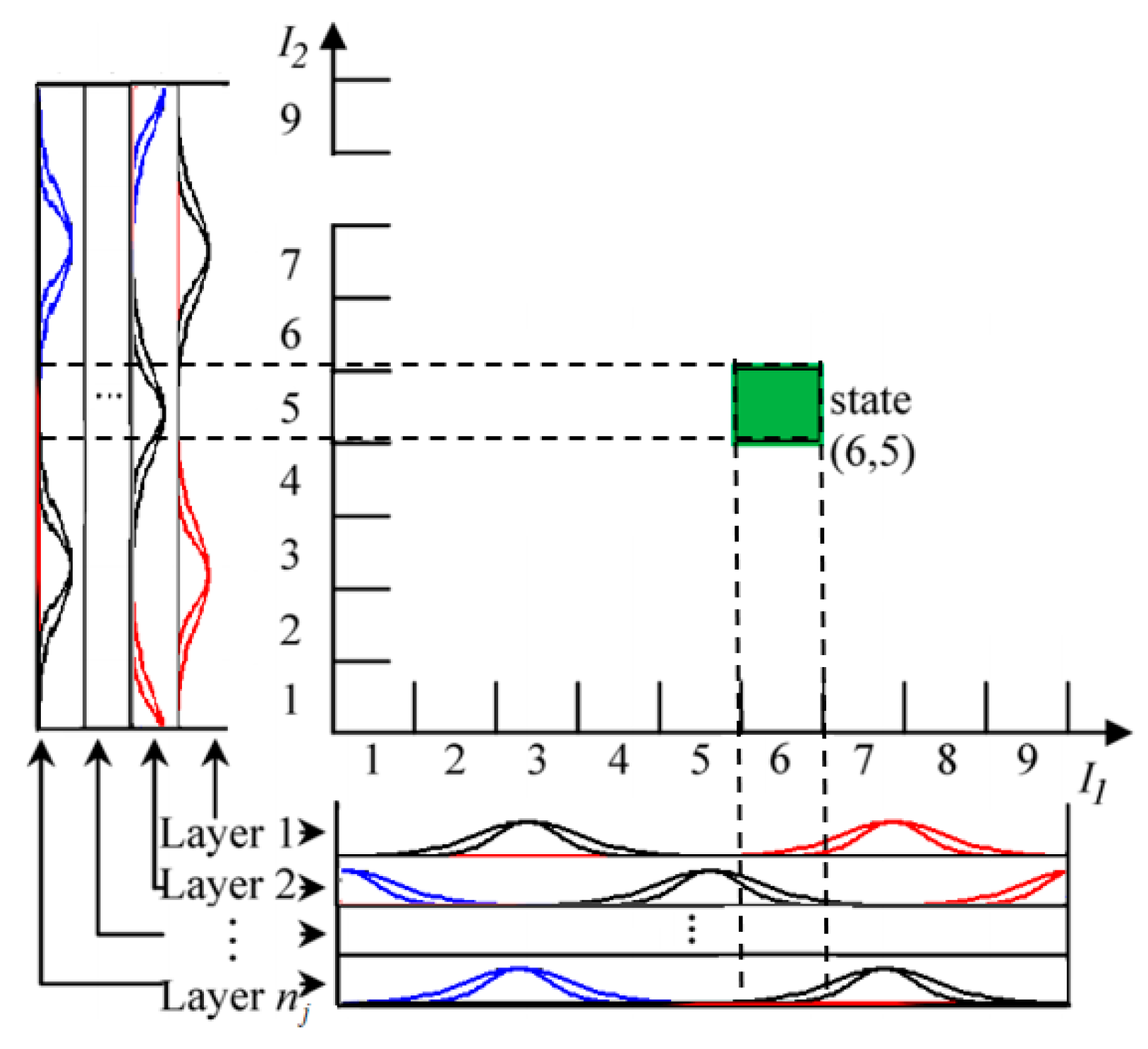
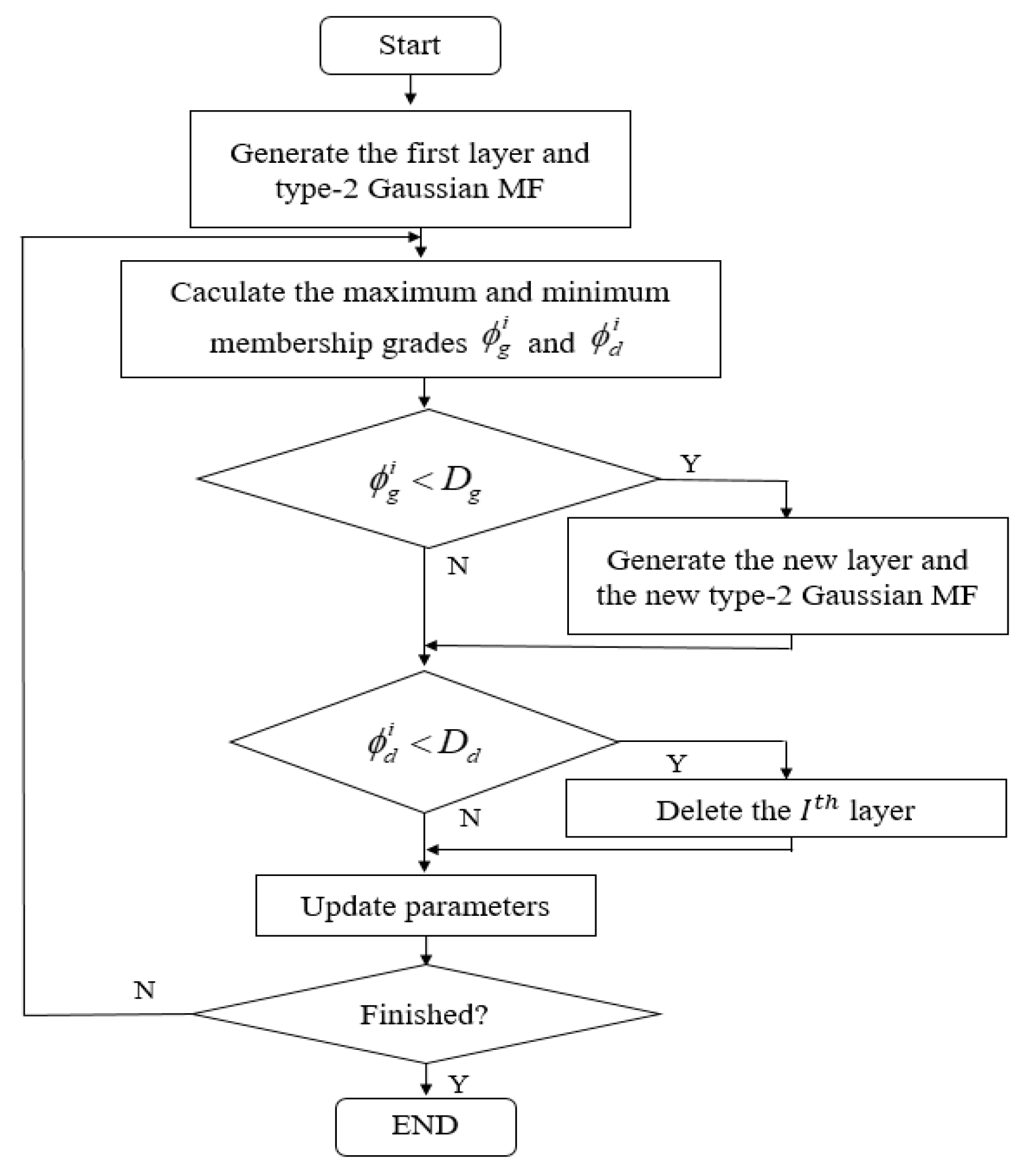
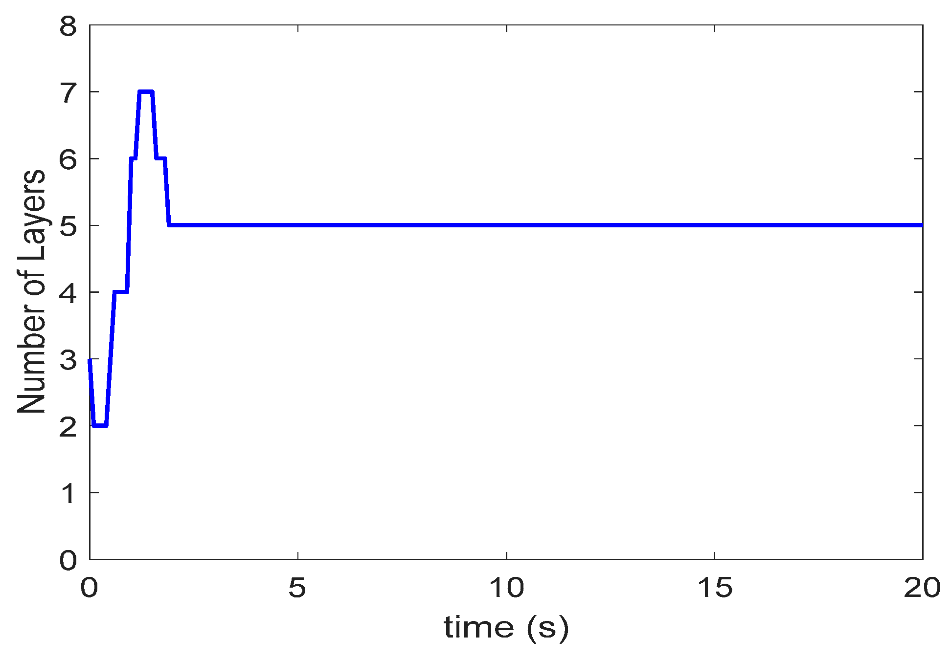
3.2. Self-Evolving Algorithm

In designing the network structure for the RIT2PC, choosing the number of layers greatly affects the control system. If the number of layers is large, huge computation times will follow; however, a few numbers of layers may not cover all cases, especially when the input changes across a wide range of values. To overcome this problem, this study presents the self-evolving algorithm to construct the layers of the proposed network autonomously. The flowchart of the self-evolving algorithm is shown in Figure 5.
The condition for generating new layers can be described as follows:
I f ( ϕ g I < D g ) T h e n           { G e n e r a t i n g a   n e w l a y e r }
ϕ g I = m a x [ μ i 11 , , μ i 1 n k , μ i 21 , , μ i 2 n k , , μ i n j 1 , , μ i n j n k ]
μ i j k = μ ¯ i j k + μ ¯ i j k 2
where ϕ g i and D g denote the maximum membership grades and the generating threshold, respectively.
The T2GMF for a new layer is given as
m i j k M ( t ) + 1 =   x i ( t )
σ ¯ i j k M ( t ) + 1 = v i n i t Δ v   and   σ ¯ i j k M ( t ) + 1 = σ i n i t + Δ σ
where M(t) denotes the number of the existing rules at time t; σ i n i t denotes the initial value of the variance; Δ σ denotes the half of the variance uncertain.
The condition for deleting unnecessary layers can be described as
I f ( ϕ d I < D d ) T h e n                     { d e l e t i n g t h e I t h l a y e r }
ϕ d I = m i n [ μ i 11 , , μ i 1 n k , μ i 21 , , μ i 2 n k , , μ i n j 1 , , μ i n j n k ]
where ϕ d i and D d denote the minimum membership grades and the deleting threshold, respectively.

3.3. Parameter Learning For SRIT2PC

Herein, we can assume there exists an optimal controller u S R I T 2 P C * such that
u * ( t ) = u S R I T 2 P C * ( w ¯ * , w ¯ * , m * , σ ¯ * , σ ¯ * , r ¯ * , r ¯ * , t ) ξ ( t )
where ξ ( t ) denotes the approximation error; w ¯ * , w ¯ * , m * , σ ¯ * , σ ¯ * , r ¯ * , r ¯ * denote the optimal parameters for w ¯ , w ¯ , m , σ ¯ , σ ¯ , r ¯ , r ¯ , respectively.
Since u S R I T 2 P C * cannot be determined, an online estimation controller, u ^ S R I T 2 P C , is used to estimate u S R I T 2 P C * . Thus, the control input is denoted as
u ^ ( t ) = u ^ S R I T 2 P C ( w ¯ ^ , w ¯ ^ , m ^ , v ^ ¯ , v ¯ ^ , r ¯ ^ , r ¯ ^ , t ) u ^ F ( t )
where w ¯ ^ , w ¯ ^ , m ^ , v ^ ¯ , v ¯ ^ , r ¯ ^ , r ¯ ^ denote the estimation of w ¯ * , w ¯ * , m * , v ¯ * , v ¯ * , r ¯ * , r ¯ * , respectively; u ^ F denotes the estimation of fuzzy compensator controller.
A high-order sliding surface can be defined as
s ( t ) = e ( n 1 ) + k 1 e ( n 2 ) + k n 0 t e ( τ ) d τ
Taking the derivative of Equation (27) and using Equation (6), the following can be obtained:
s ˙ ( t ) = e ( n ) + K T e   = A e ( t ) + d ( t ) + Δ f ( t ) + u ( t ) + K T e
The Lyapunov function can be described as
  V 1 ( s ( t ) ) = 1 2 s 2 ( t )
Taking the derivative of Equation (29) and using Equations (26) and (28), the following can be obtained:
V ˙ 1 ( t ) = s ( t ) s ˙ ( t ) = s ( t ) [ e ( n ) + K T e ] = s ( t ) [ A e ( t ) + d ( t ) + Δ f ( t ) + ( u ^ S R I T 2 P C ( w ¯ ^ , w ¯ ^ , m ^ , v ^ ¯ , v ¯ ^ , r ¯ ^ , r ¯ ^ , t ) u ^ F ( t ) ) + K T e ]
Using the gradient descent method, the parameter-updating laws for SRIT2PC can be obtained as follows:
w ¯ ^ j k ( t + 1 ) = w ¯ ^ j k ( t ) η ^ w V ˙ 1 ( t ) w ¯ ^ j k = w ¯ ^ j k ( t ) η ^ w V ˙ 1 ( t ) u ^ S R I T 2 P C k u ^ S R I T 2 P C k y k l y k l w ¯ ^ j k = w ¯ ^ j k ( t ) 1 2 η ^ w s ( t ) f ¯ j k
w ¯ ^ j k ( t + 1 ) = w ¯ ^ j k ( t ) η ^ w V ˙ 1 ( t ) w ¯ ^ j k = w ¯ ^ j k ( t ) η ^ w V ˙ 1 ( t ) u ^ S R I T 2 P C k u ^ S R I T 2 P C k y k r y k r w ¯ ^ j k = w ¯ ^ j k ( t ) 1 2 η ^ w s ( t ) f ¯ j k
m ^ i j k ( t + 1 ) = m ^ i j k ( t ) η ^ m V ˙ 1 ( t ) m ^ i j k = m ^ i j k ( t ) η ^ m V ˙ 1 ( t ) u ^ S R I T 2 P C k ( u ^ S R I T 2 P C k y k l y k l f ¯ j k f ¯ j k μ ¯ i j k μ ¯ i j k m ^ i j k + u ^ S R I T 2 P C y k r y k r ϕ ¯ j k f ¯ j k μ ¯ i j k μ ¯ i j k m ^ i j k )
σ ¯ ^ i j k ( t + 1 ) = σ ¯ ^ i j k ( t ) η ^ σ V ˙ 1 ( t ) σ ¯ ^ i j k = σ ¯ ^ i j k ( t ) η ^ σ ( V ˙ 1 ( t ) u ^ S R I T 2 P C k u ^ S R I T 2 P C k y ^ k l y ^ k l f ¯ j k f ¯ j k μ ¯ i j k μ ¯ i j k σ ¯ ^ i j k ) = σ ¯ ^ i j k ( t ) η ^ σ s ( t ) f ¯ j k w ¯ j k ( I i m ^ i j k ) 2 σ ^ ¯ i j k 3
σ ¯ ^ i j k ( t + 1 ) = σ ¯ ^ i j k ( t ) η ^ σ V ˙ 1 ( t ) σ ¯ ^ i j k = σ ¯ ^ i j k ( t ) η ^ σ ( V ˙ 1 ( t ) u ^ S R I T 2 P C k u ^ S R I T 2 P C k y ^ k r y ^ k r f ¯ j k f ¯ j k μ ¯ i j k μ ¯ i j k σ ¯ ^ i j k ) = σ ¯ ^ i j k ( t ) η ^ σ s ( t ) f ¯ j k w ¯ j k ( I i m ^ i j k ) 2 σ ¯ ^ i j k 3
r ^ ¯ i j k ( t + 1 ) = r ^ ¯ i j k ( t ) η ^ r V ˙ 1 ( t ) r ^ ¯ i j k = r ^ ¯ i j k ( t ) η ^ σ ( V ˙ 1 ( t ) u ^ S R I T 2 P C k u ^ S R I T 2 P C k y ^ k l y ^ k l f ¯ j k f ¯ j k μ ¯ i j k μ ¯ i j k I ^ ¯ r i I ^ ¯ r i r ^ ¯ i j k ) = r ^ ¯ i j k ( t ) + 1 2 η ^ r s ( t ) f ¯ j k w ¯ j k μ ¯ i j k ( I i m ^ i j k ) σ ^ ¯ i j k 2
r ¯ ^ i j k ( t + 1 ) = r ¯ ^ i j k ( t ) η ^ r V ˙ 1 ( t ) r ¯ ^ i j k = r ¯ ^ i j k ( t ) η ^ σ ( V ˙ 1 ( t ) u ^ S R I T 2 P C k u ^ S R I T 2 P C k y ^ k r y ^ k r f ¯ j k f ¯ j k μ ¯ i j k μ ¯ i j k I ¯ ^ r i I ¯ ^ r i r ¯ ^ i j k ) = r ¯ ^ i j k ( t ) + 1 2 η ^ r s ( t ) f ¯ j k w ¯ j k μ ¯ i j k ( I i m ^ i j k ) σ ¯ ^ i j k 2
where the positive learning-rates are denoted by η ^ w , η ^ m , η ^ σ , η ^ r .

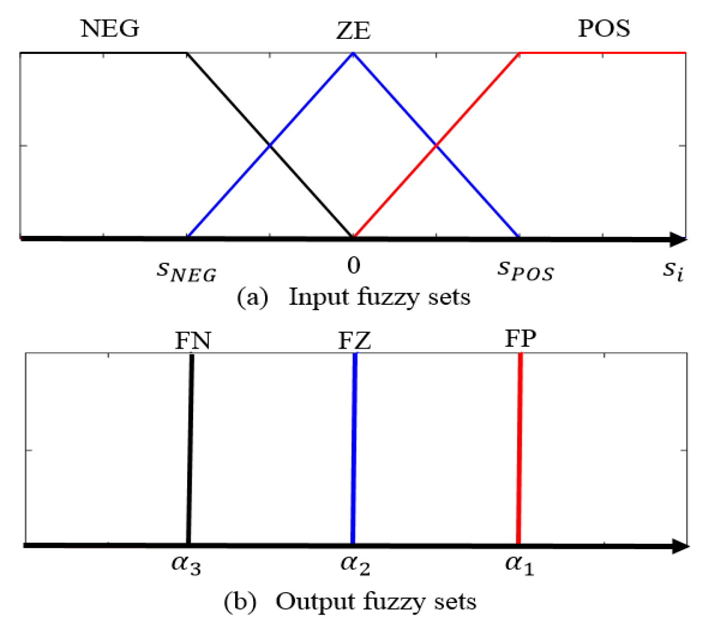
3.4. Compensator Controller

To address the approximation error, a simple fuzzy compensator controller can be proposed as follows:
R 1 : I f s i i s P O S , t h e n u F i i s F P R 2 : I f s i i s Z E , t h e n u F i i s F Z R 3 : I f s i i s N E G , t h e n u F i i s F N
where POS, ZE, and NEG denote the positive, zero, and negative inputs of the MFs, respectively; FP, FZ, and FN denote the positive, zero, and negative outputs the MFs, respectively; s i and u F i denote the control input and control output, respectively.
Figure 6 shows the input and output MFs of the fuzzy compensator controller. Using the center-of-gravity method, the control output is given by
u F i = a = 1 3 α a i β a i a = 1 3 β a i = α 1 i β 1 i + α 2 i β 2 i + α 3 i β 3 i
where α i = [ α 1 i , α 2 i , α 3 i ] denotes the weight vector of the fuzzy rules and β i = [ β 1 i , β 2 i , β 3 i ] denotes the firing-strengths vector of the fuzzy rules, which is given by
C a s e 1 : ( s i ϑ ) β 1 i = 0 ; β 2 i = 0 ; β 3 i = 1 ; C a s e 2 : ( ϑ s i 0 ) β 1 i = 0 ; β 2 i = ( s i + ϑ ) / ϑ ; β 3 i = 1 β 2 i ; C a s e 3 : ( 0 s i ϑ ) β 1 i = 1 β 2 i ; β 2 i = ( ϑ s i ) / ϑ ; β 3 i = 0 ; C a s e 4 : ( s i > ϑ ) β 1 i = 1 ; β 2 i = 0 ; β 3 i = 0 ;
where ϑ is the parameter for defining the firing strengths.
By choosing the triangular membership function for the input shown in Figure 6, we can obtain β 1 i + β 2 i + β 3 i = 1 . Using a singleton membership function for the output, letting α 1 i = α ^ i , α 2 i = 0 , α 3 i = α ^ i , and rewriting Equation (39) using α i = [ α ^ i , 0 , α ^ i ] , the following can be obtained:
u F i = α ^ i ( β 1 i β 3 i )
Rewriting Equation (30) and using Equations (25), (26), and (41), the following can be obtained:
V ˙ 1 = i = 1 m [ s i ( t ) ξ i ( t ) s i ( t ) α ^ i ( β 1 i β 3 i ) ] i = 1 m [ | s i ( t ) | . | ξ i ( t ) | s i ( t ) α ^ i ( β 1 i β 3 i ) ] = i = 1 m [ | s i ( t ) | . | ξ i ( t ) | α ^ i | s i ( t ) | . | β 1 i β 3 i | ] = i = 1 m [ | s i ( t ) | . | β 1 i β 3 i | ] ( α ^ i | ξ i ( t ) | | β 1 i β 3 i | )
where m denotes the dimension of vector s i . In Equation (42), if there exists an estimated value α ^ i > | ξ i ( t ) | | β 1 i β 3 i | , then V ˙ 0 is satisfied. An optimal value α i * can be defined to achieve a minimum value of α ^ i with the following equation:
α i * = | ξ i ( t ) | | β 1 i β 3 i | + Ω i
where Ω i denotes a positive constant.
The estimation-error vector can be described as α ˜ i = [ α ˜ 1 , , α ˜ i , , α ˜ m ] T , where α ˜ i is given as
α ˜ i = α i * α ^ i
Accordingly, the Lyapunov function can be defined as
V 2 ( s ( t ) ) = 1 2 s T ( t ) s ( t ) + 1 2 α ˜ T α ˜
Taking the derivative of Equation (45) and using Equations (7), (25), (30), and (41), the following can be obtained:
= i = 1 m [ s i ( t ) [ u i * ( t ) ] + s i ( t ) [ u ^ S R I T 2 P C i ( t ) u ^ F i ( t ) ] + α ˜ i α ˜ ˙ i ] = i = 1 m [ s i ( t ) [ ξ ( t ) u ^ S R I T 2 P C i ( t ) ] + s i ( t ) [ u ^ S R I T 2 P C i ( t ) u ^ F i ( t ) ] + α ˜ i α ˜ ˙ i ] = i = 1 m [ s i ( t ) ξ i ( t ) α ^ i s i ( t ) ( β 1 i β 3 i ) + α ˜ i α ˜ ˙ i ] i = 1 m [ | s i ( t ) | . | ξ i ( t ) | + α ˜ i s i ( t ) ( β 1 i β 3 i ) α i * | s i ( t ) | . | β 1 i β 3 i | + α ˜ i α ˜ ˙ i ] = i = 1 m [ | s i ( t ) | . | ξ i ( t ) | + α ˜ i [ s i ( t ) ( β 1 i β 3 i ) + α ˜ ˙ i ] α i * | s i ( t ) | . | β 1 i β 3 i | ]
The estimation laws can be described as
α ^ ˙ i = α ˜ ˙ i = s i ( t ) ( β 1 i β 3 i )
Accordingly, rewriting Equation (46) and using Equation (43), the following can be obtained:
V ˙ 2 ( s ( t ) ) i = 1 m [ | s i ( t ) | . | ξ i ( t ) | | s i ( t ) | | β 1 i β 3 i | ( | ξ i ( t ) | | β 1 i β 3 i | + Ω i ) ] = i = 1 m [ | s i ( t ) | . | ξ i ( t ) | | s i ( t ) | ( | ξ i ( t ) | + Ω i | β 1 i β 3 i | ) ] = i = 1 m Ω i | s i ( t ) | | β 1 i β 3 i |
Since V ˙ 2 ( s ( t ) ) is a negative semidefinite, the stability of the proposed SRIT2PC control system can be guaranteed by the Lyapunov stability theorem.

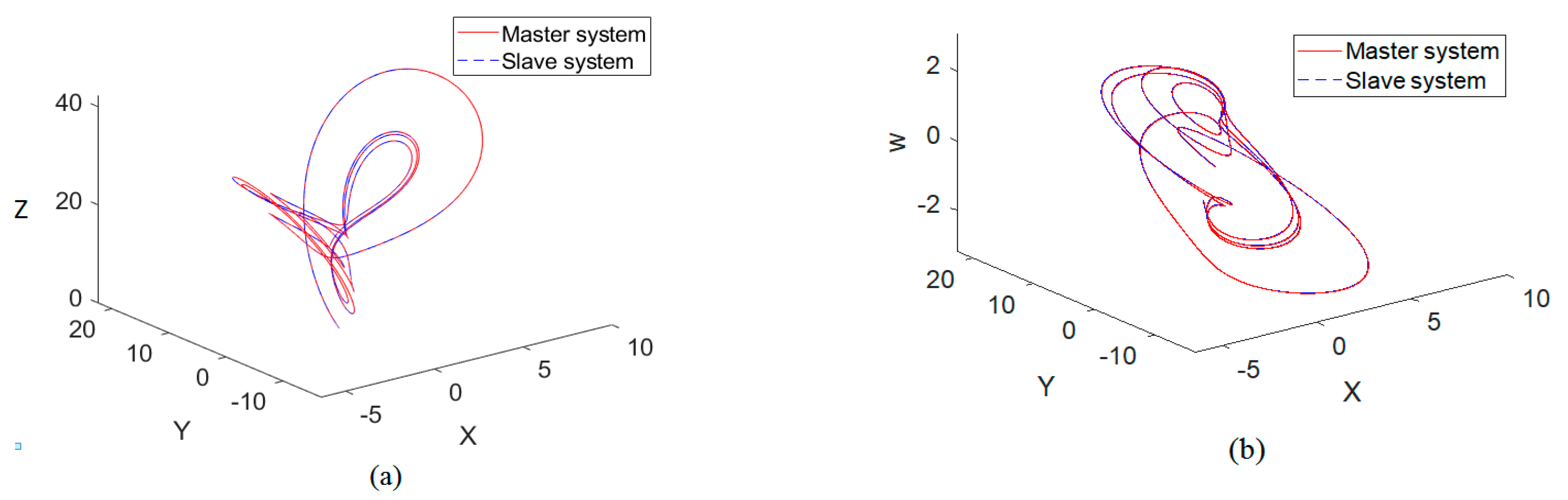
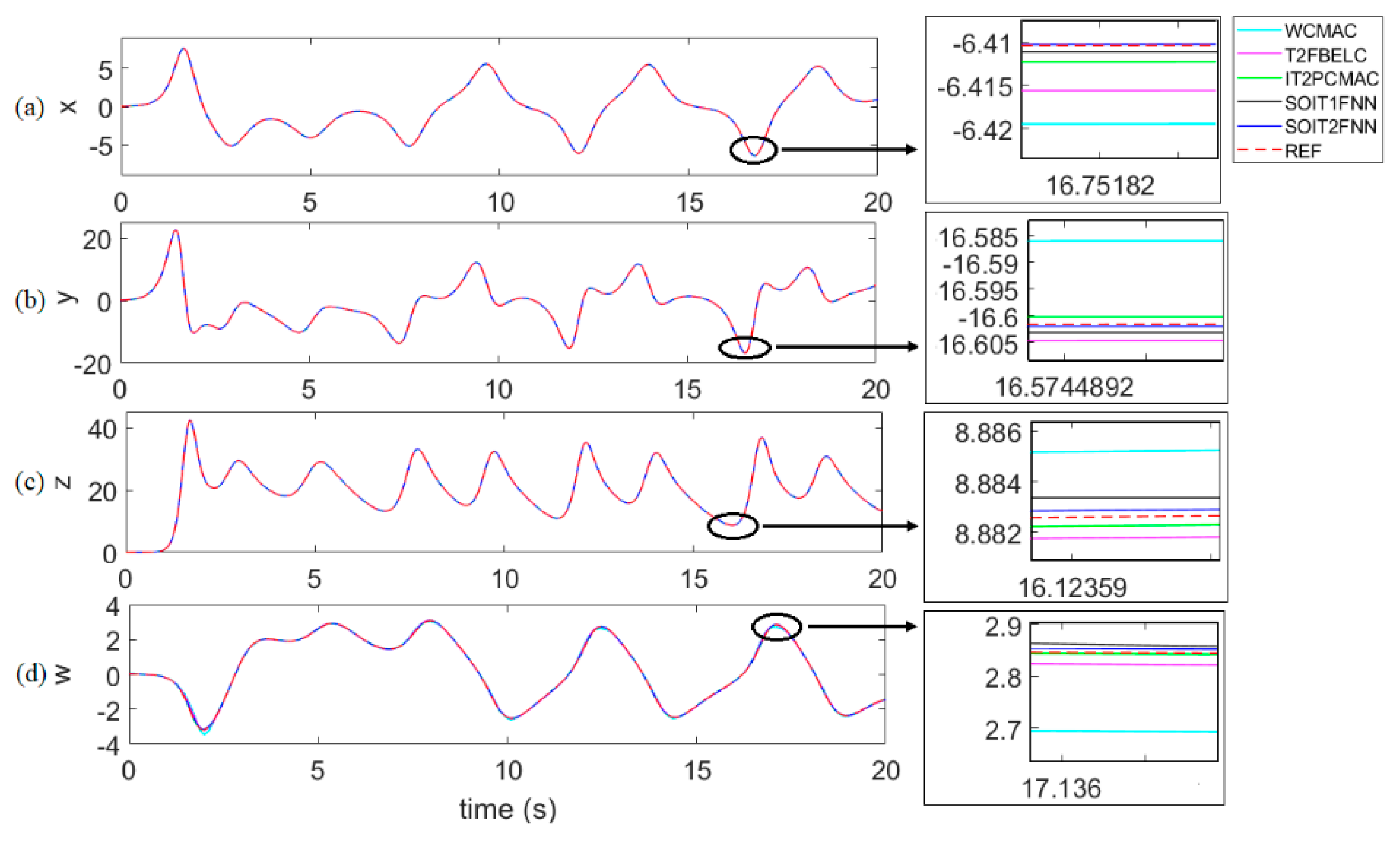
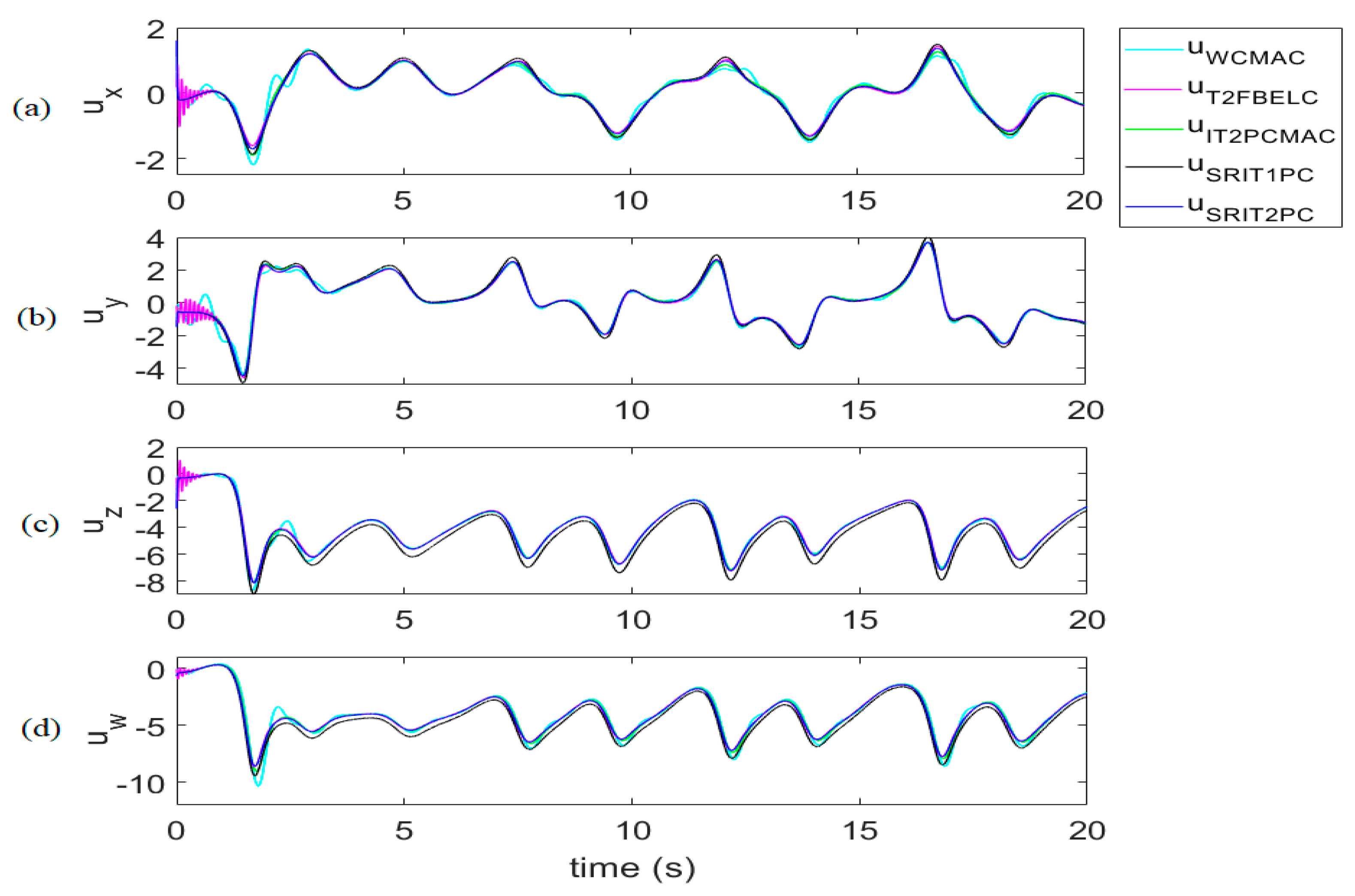
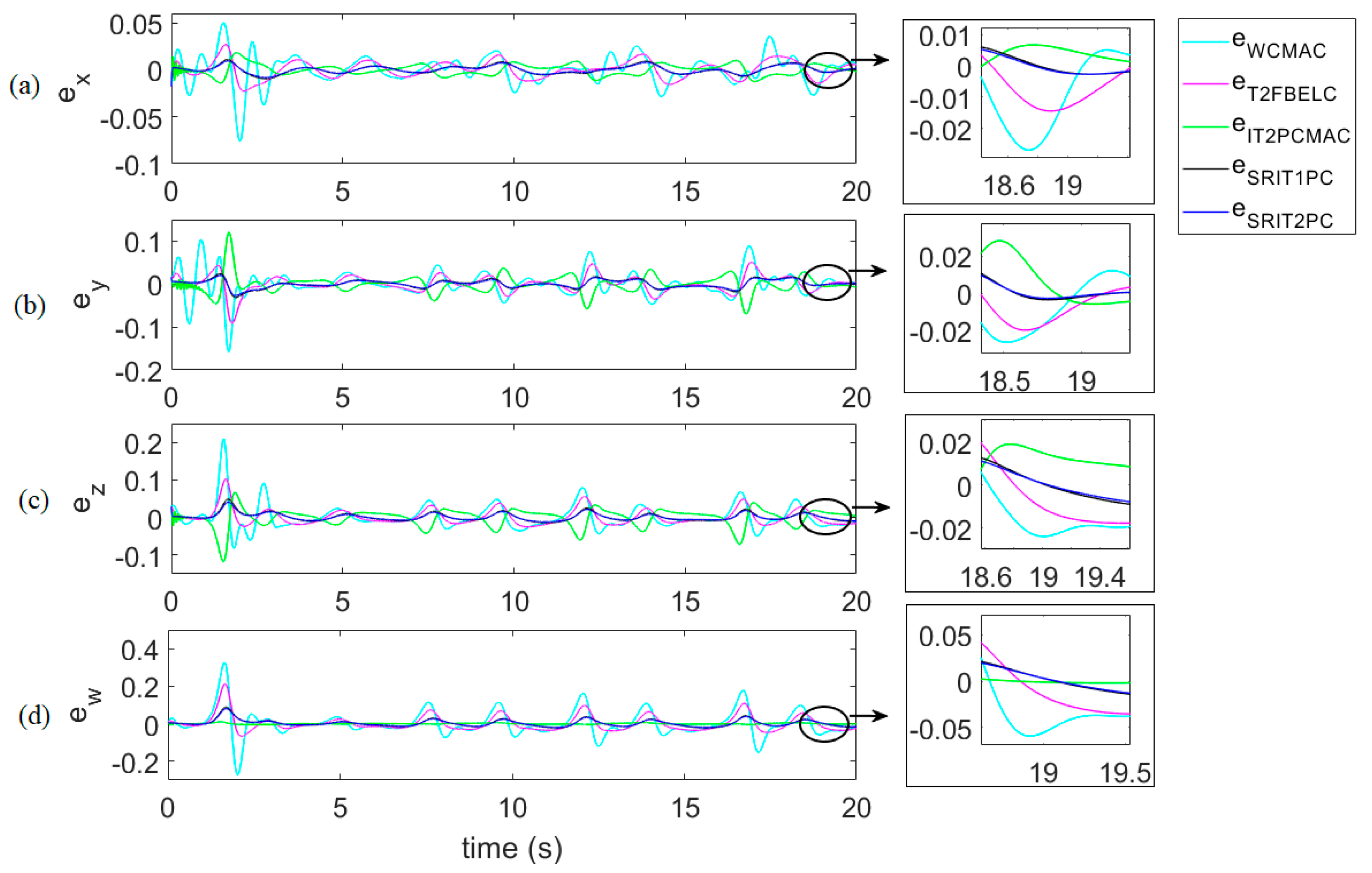
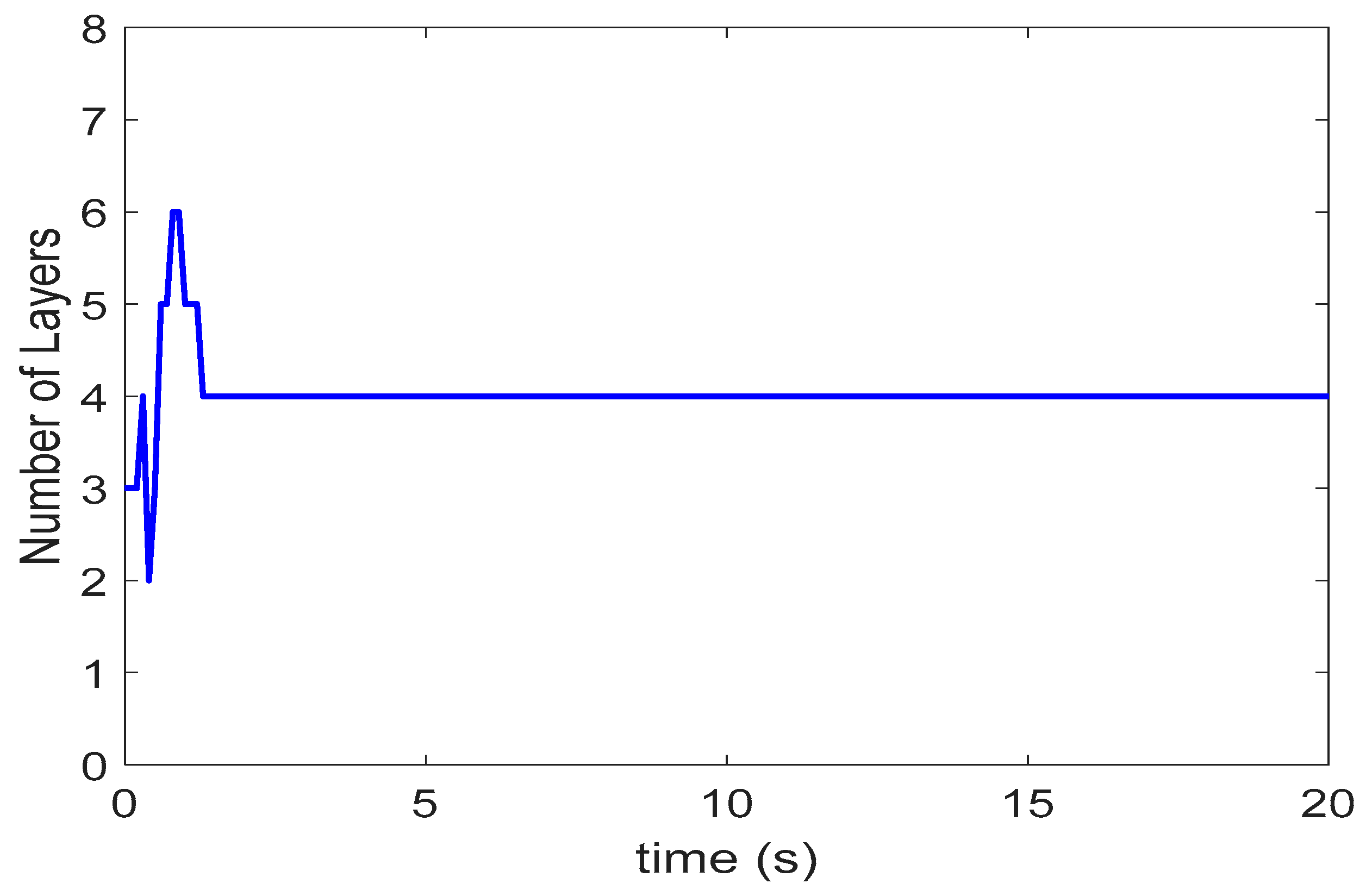
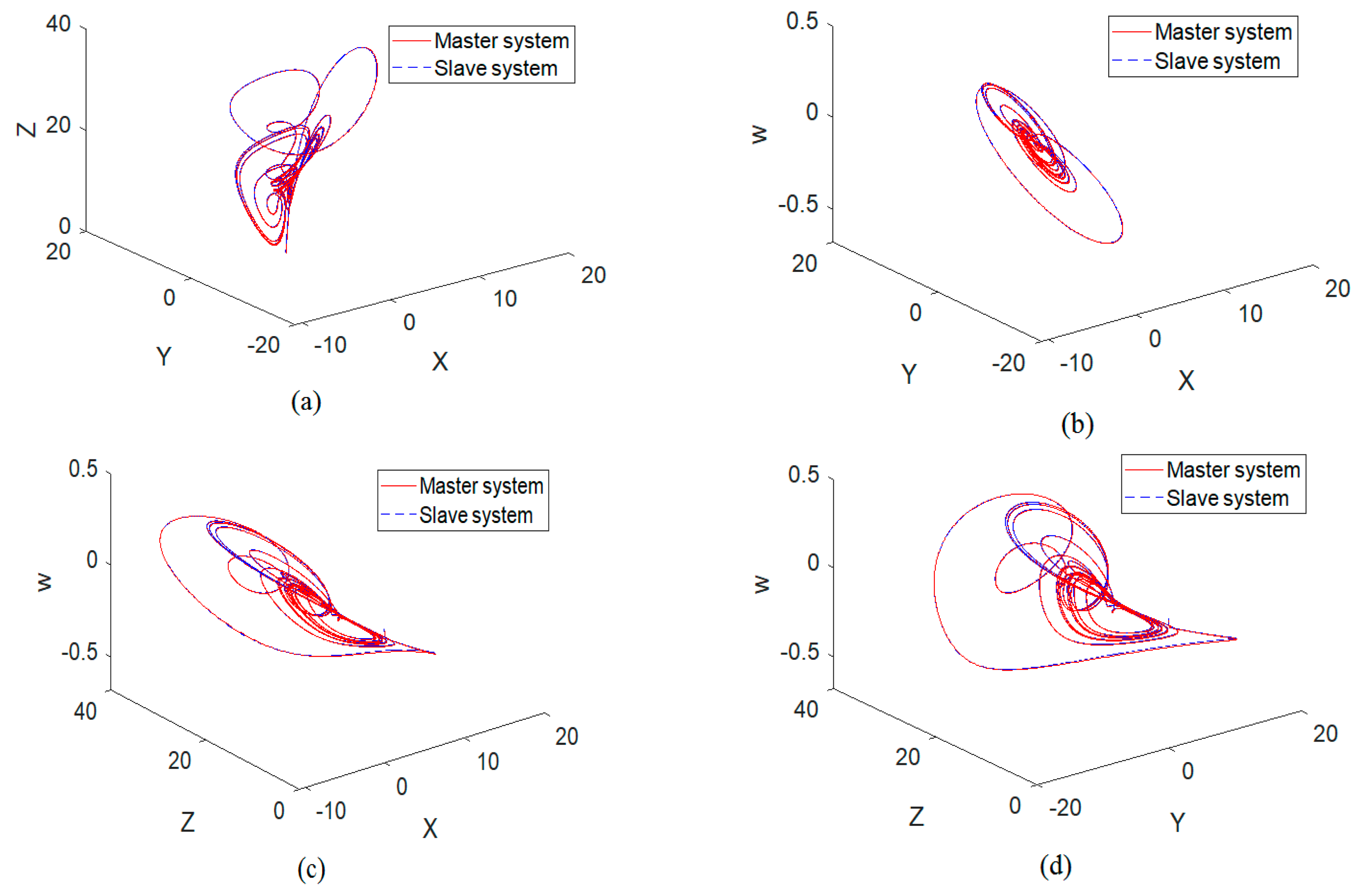
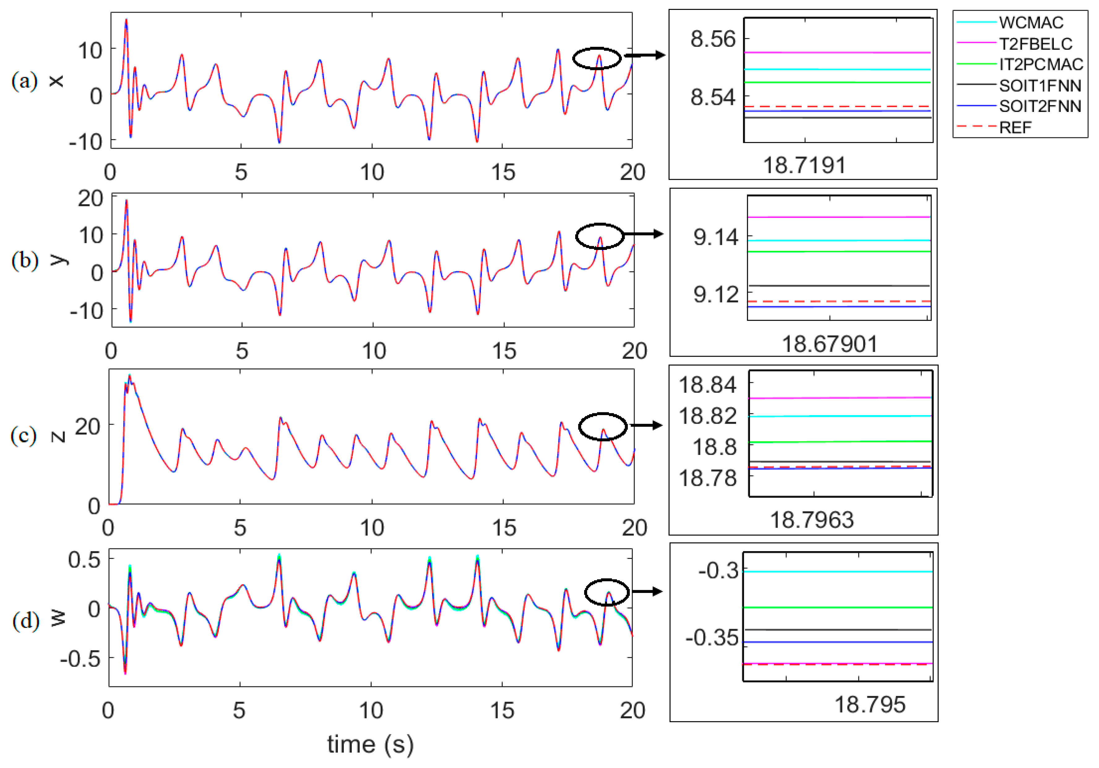
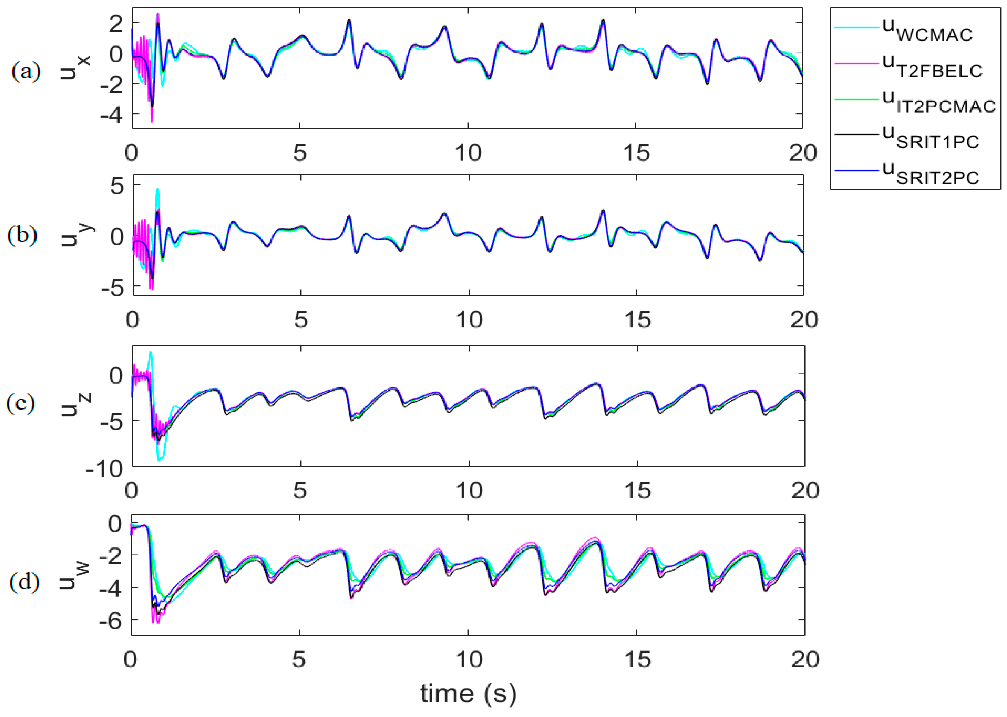
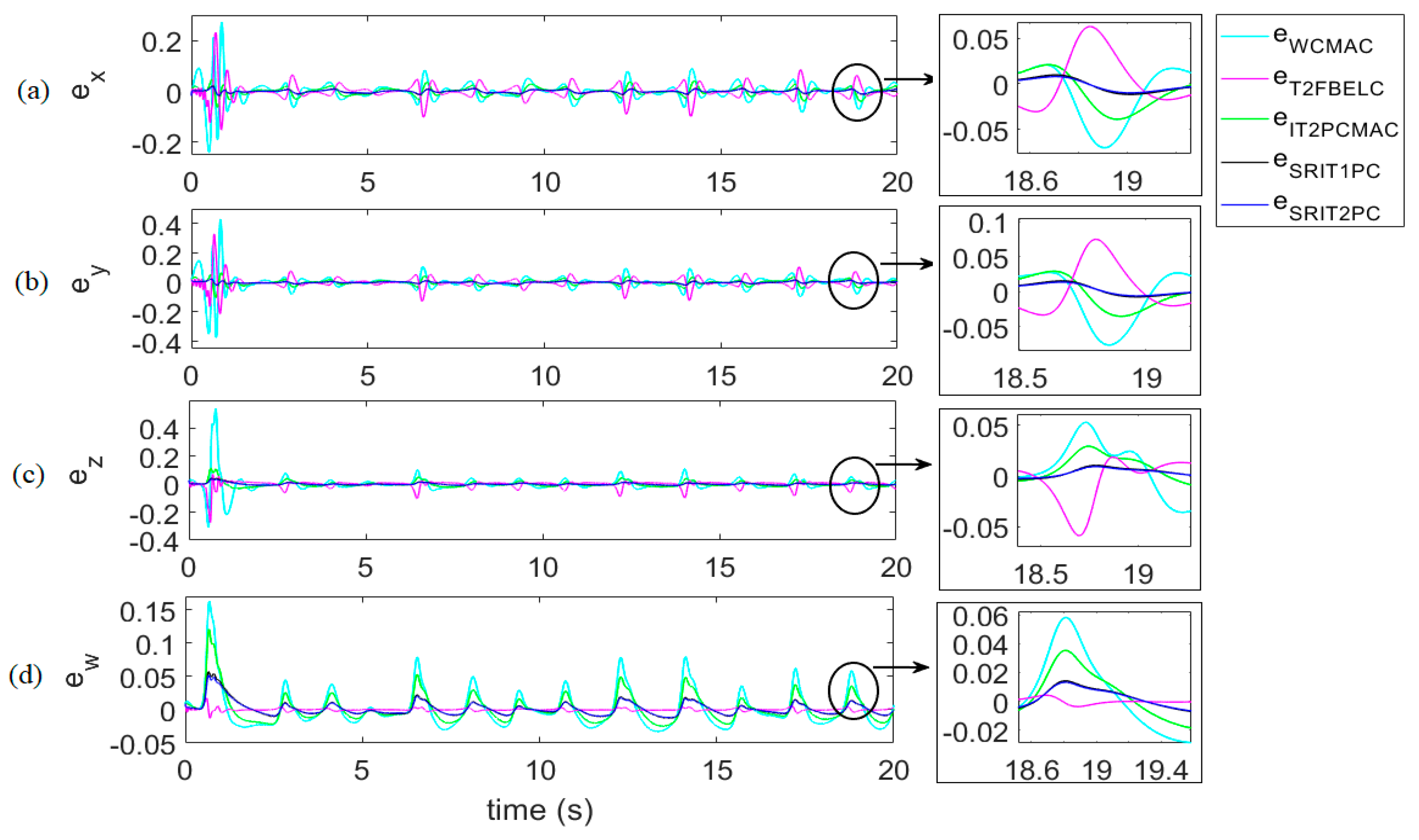
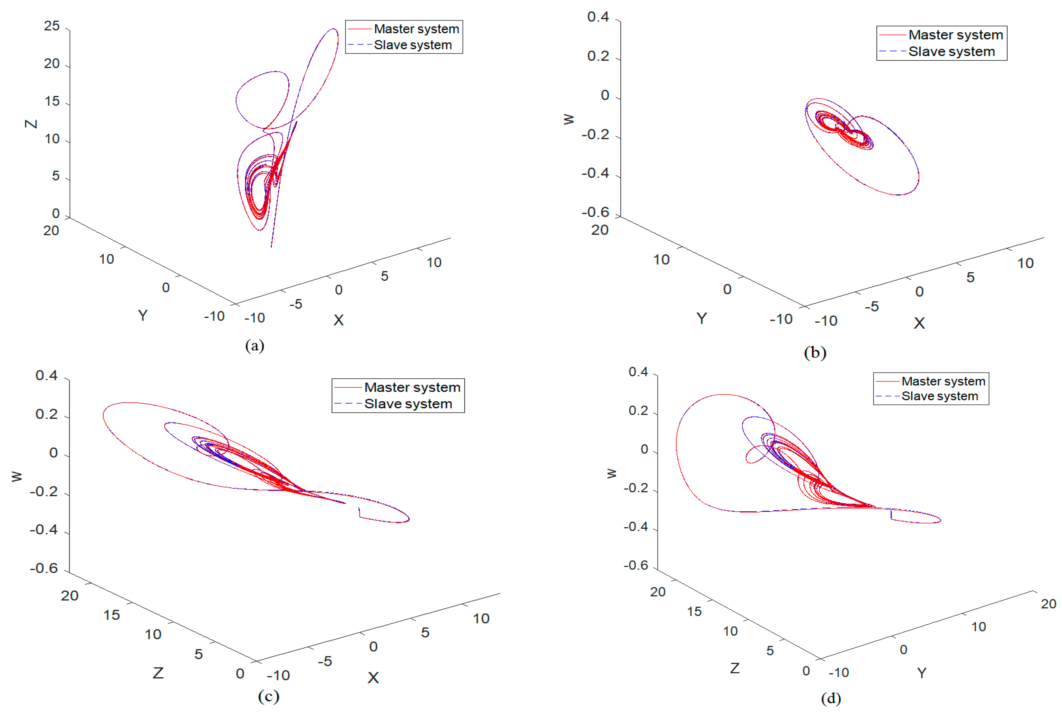
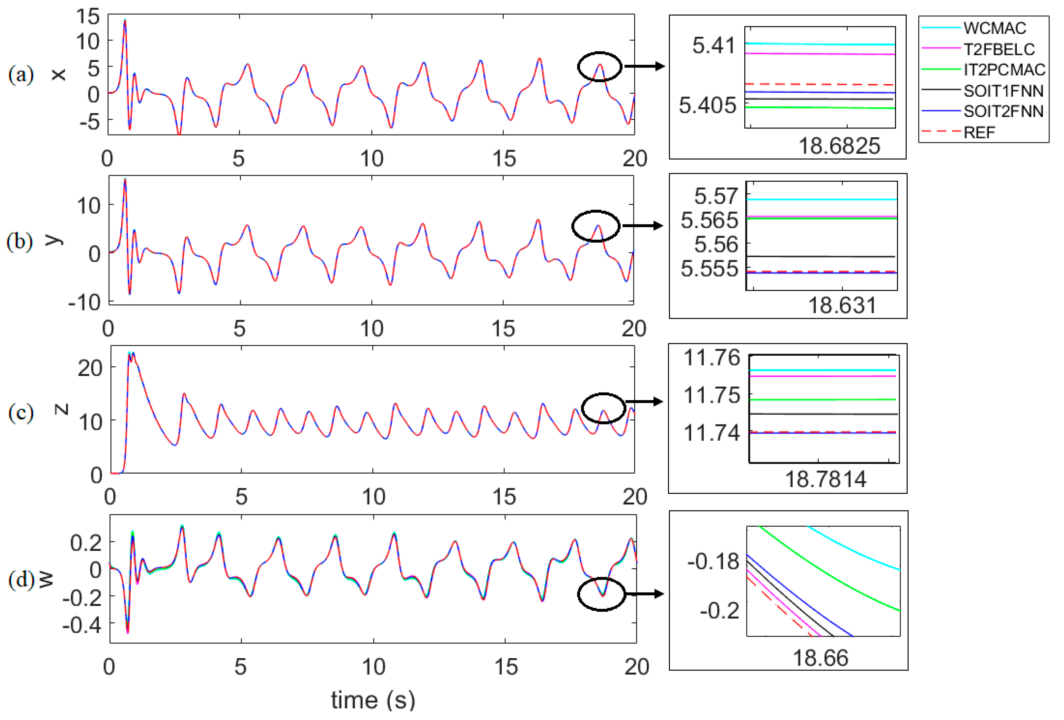
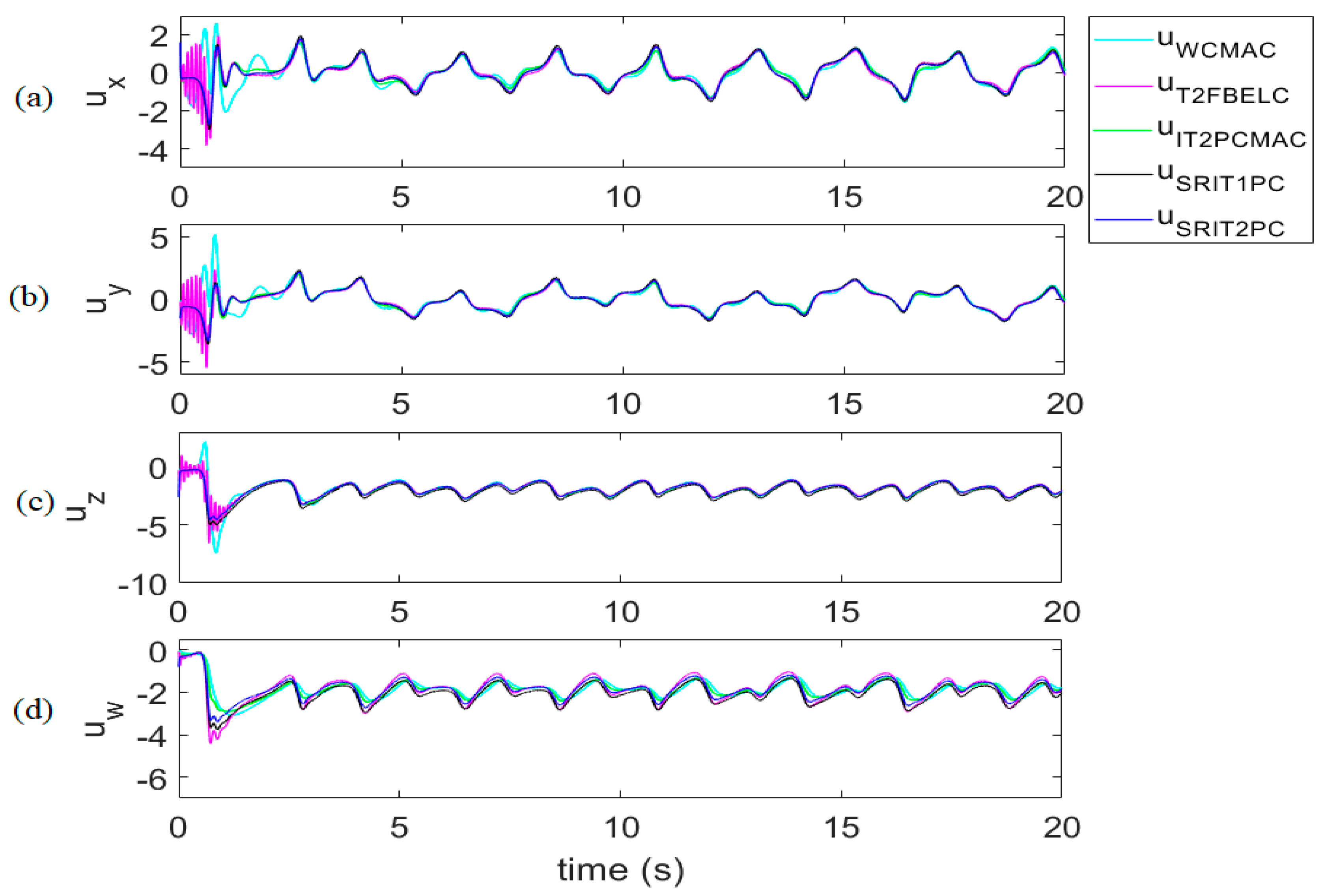
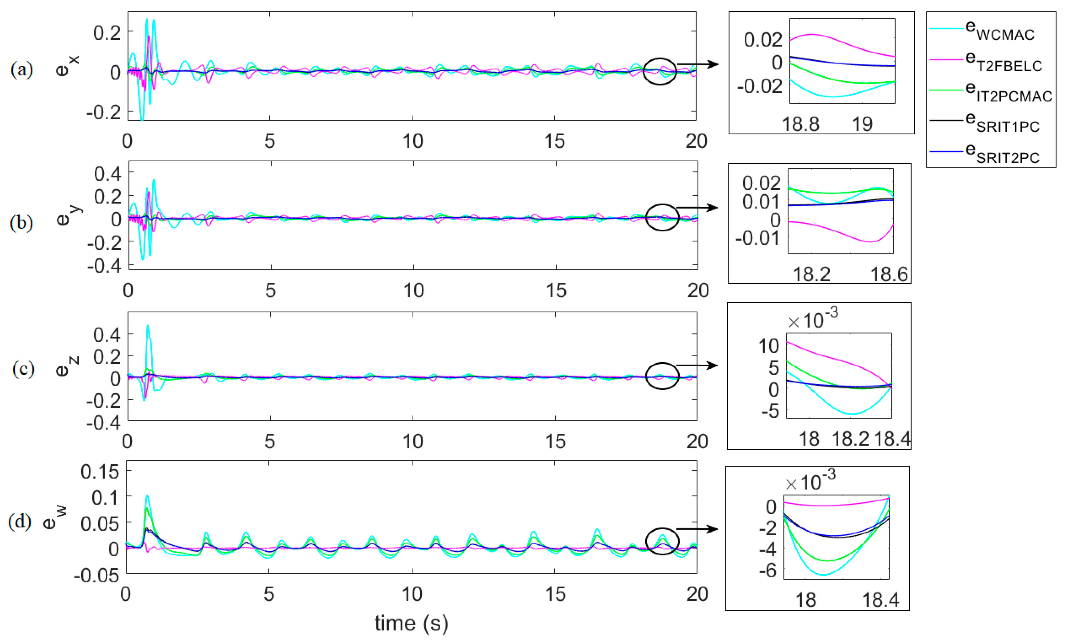
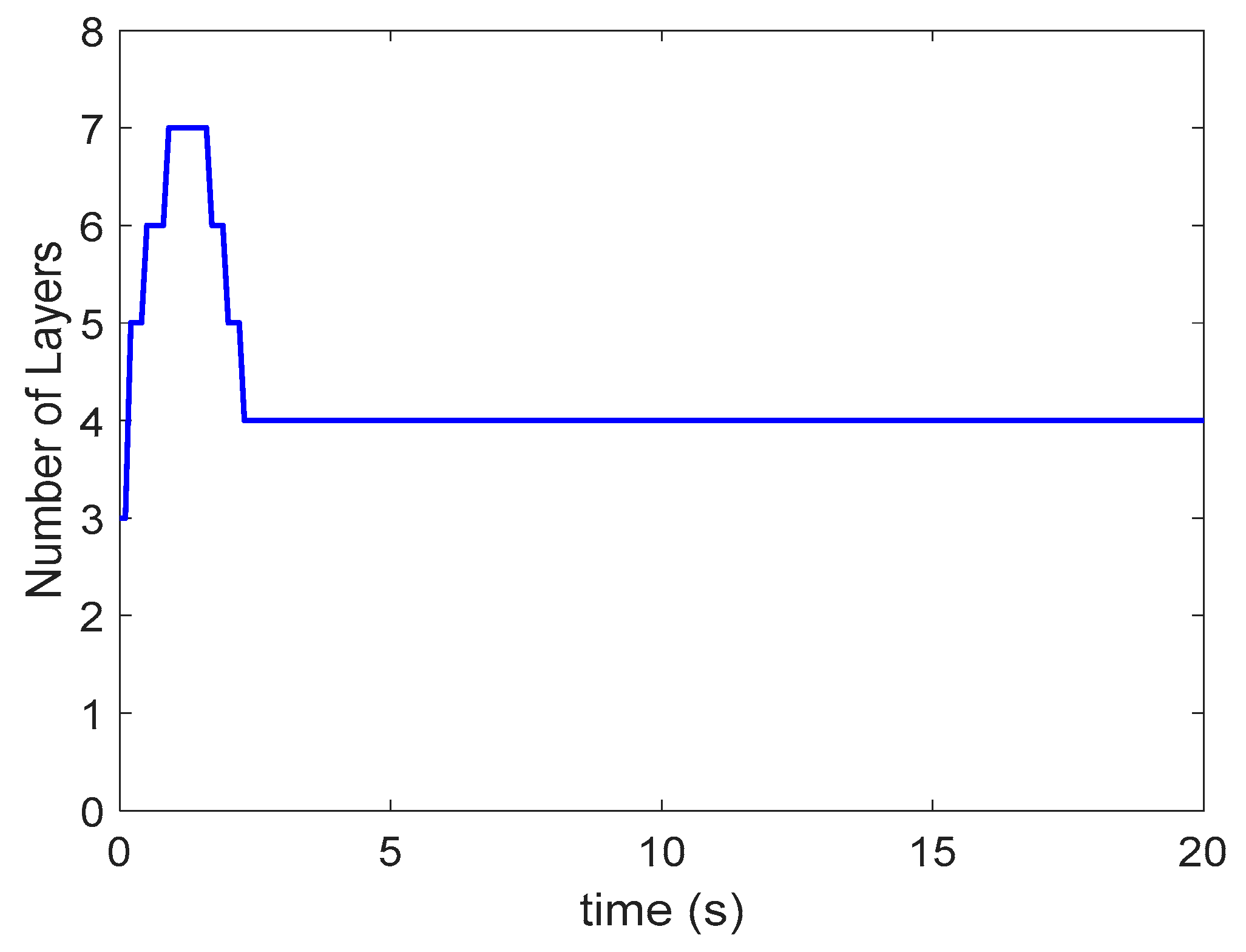
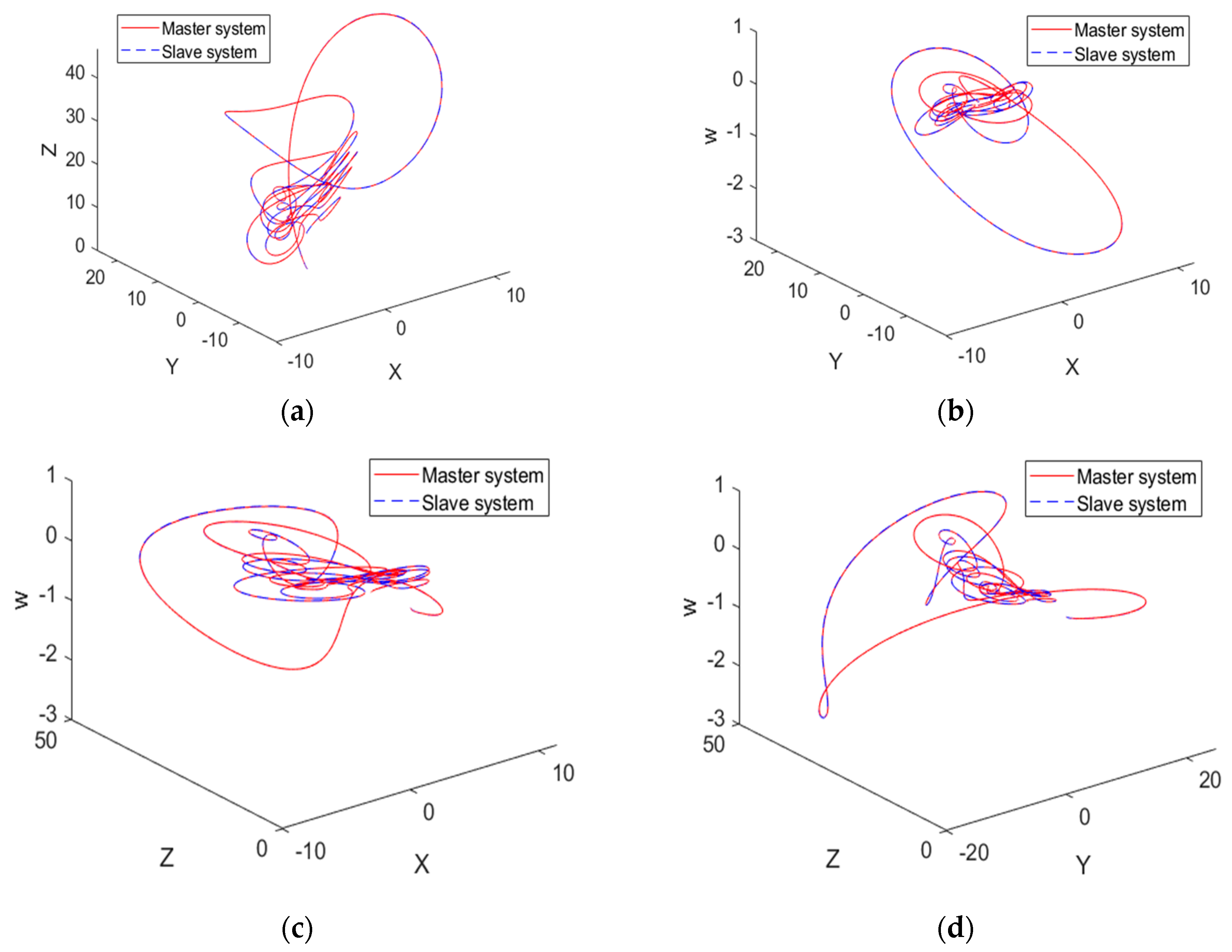
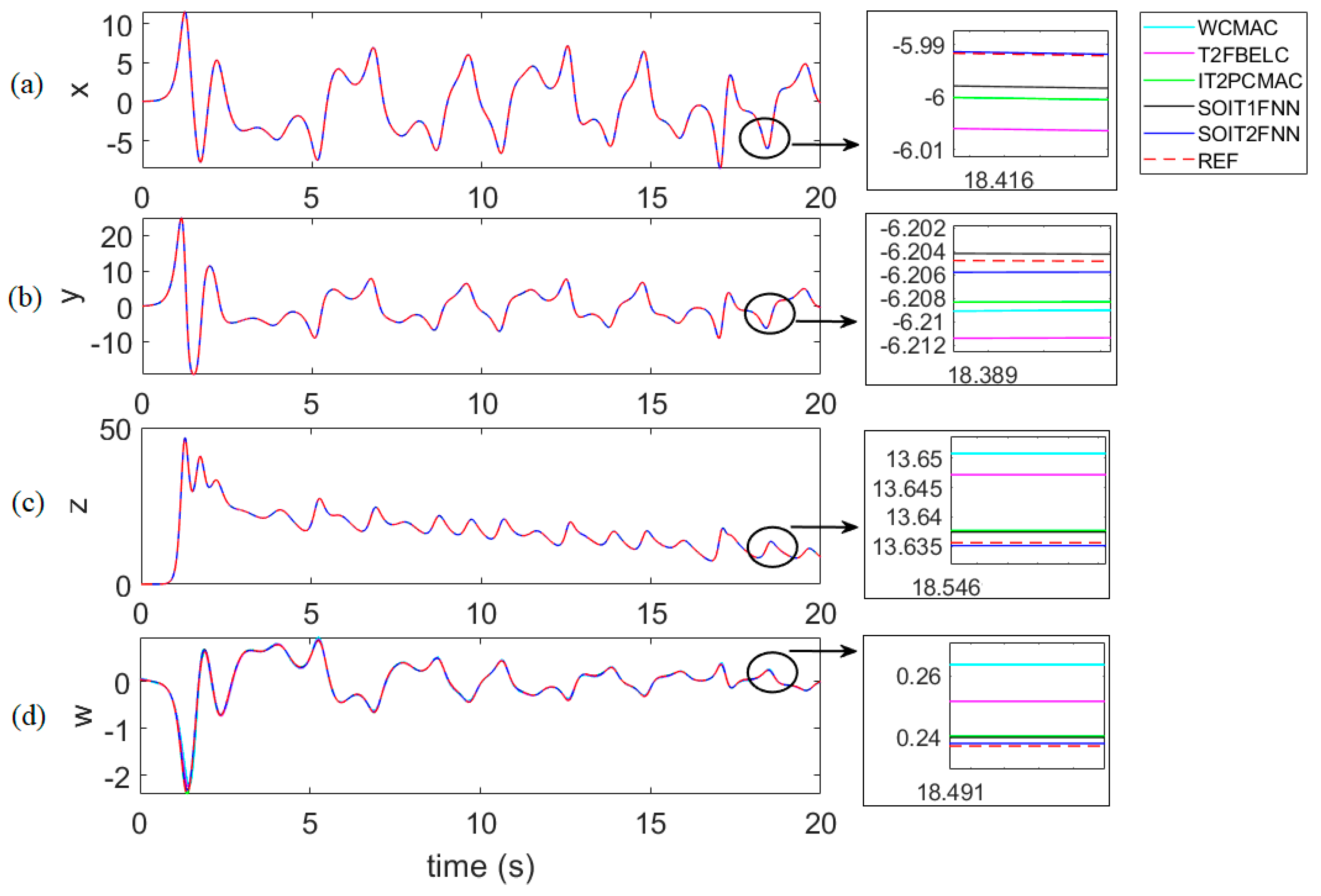
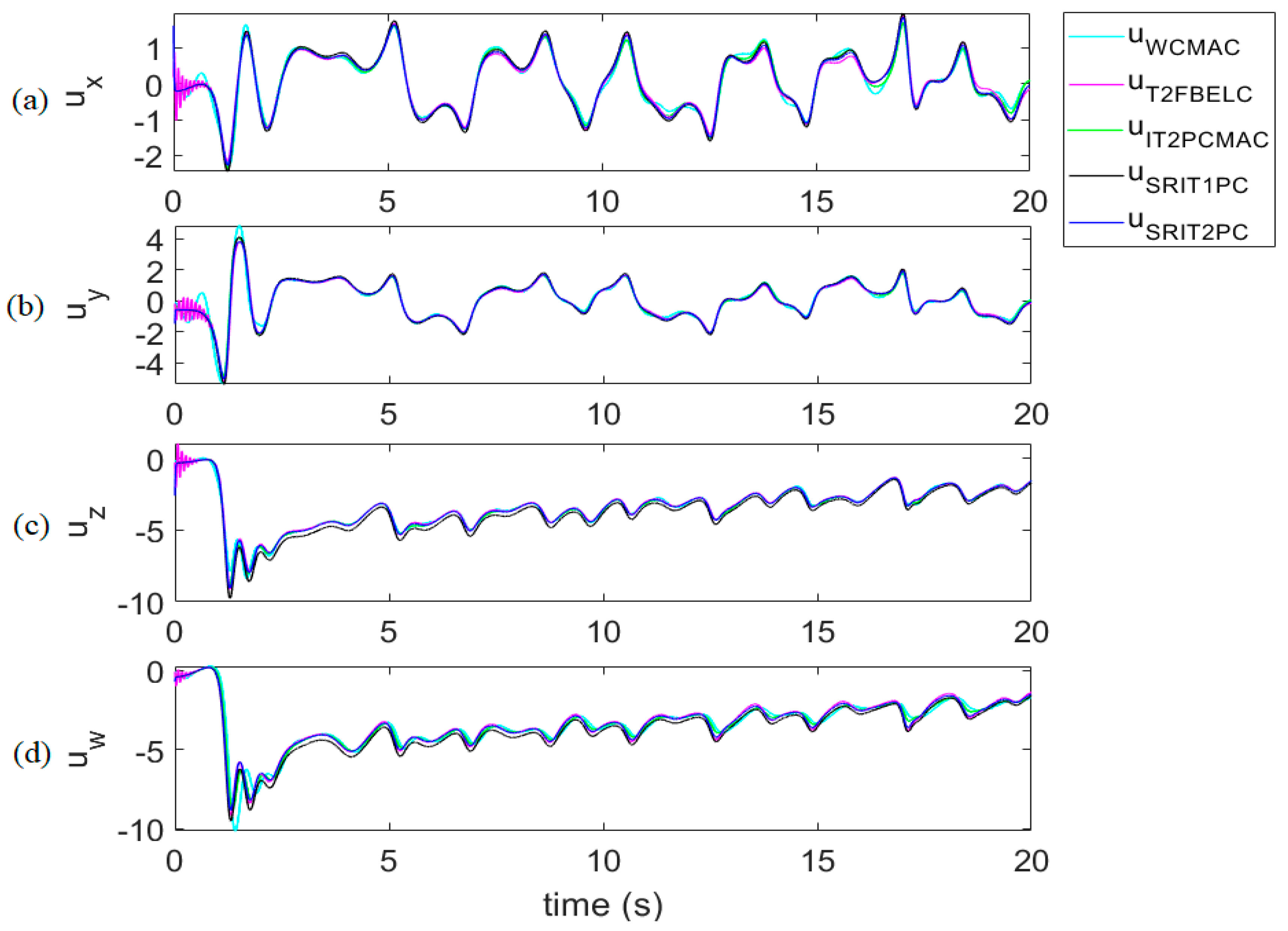
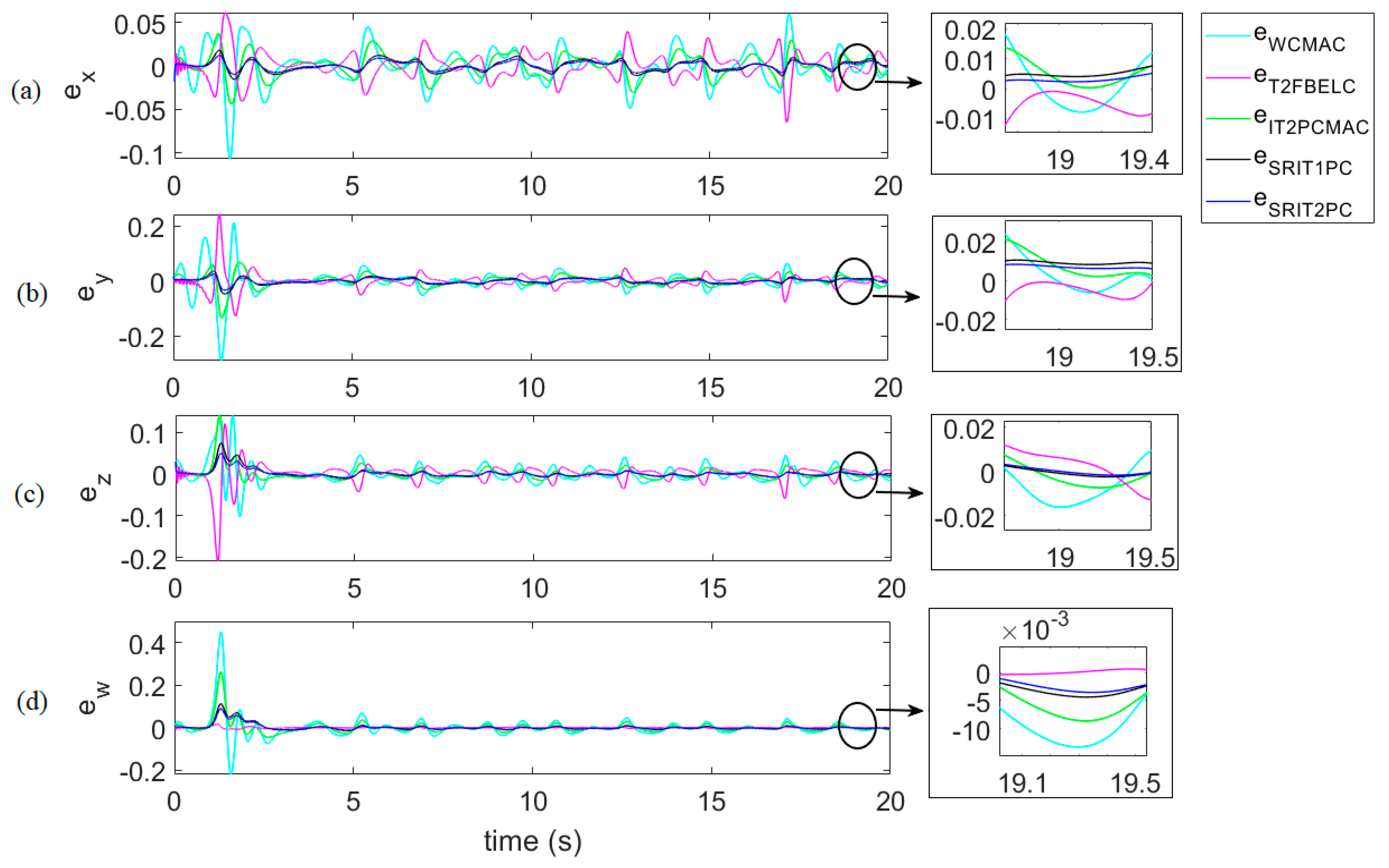
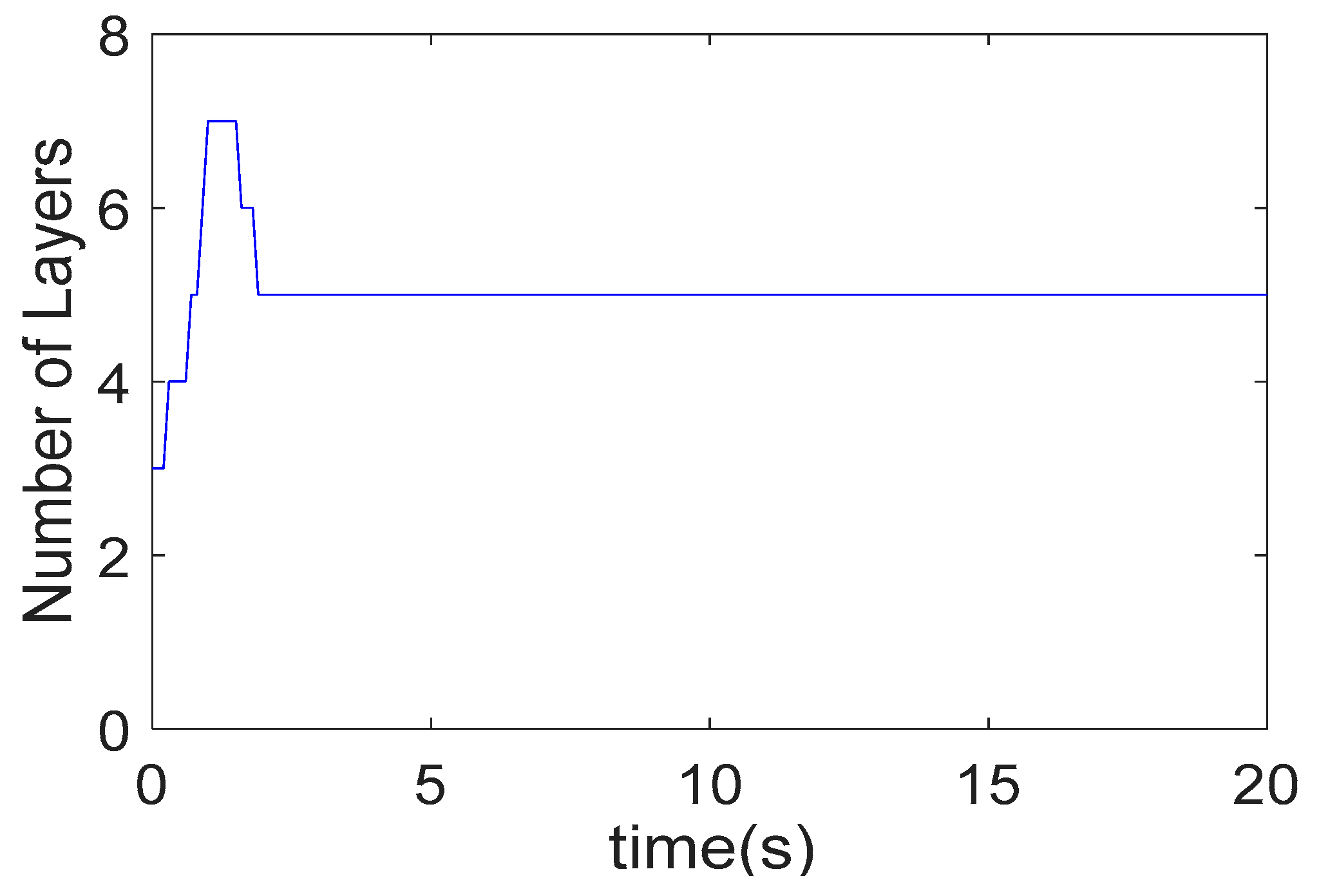
4. Illustrative Examples

To verify the feasibility and effectiveness of the proposed controller, an illustrative example is used to describe the Lorenz–Stenflo chaotic system. Using the proposed parameter-adaptive laws, the control signals, u ^ x ( t ) , u ^ y ( t ) , u ^ z ( t ) , u ^ w ( t ) , can be obtained, after which point the synchronization of the slave and the master chaotic can be obtained. The initial positions for the chaotic system are [ x 1 , y 1 , z 1 , w 1 ] = [ 0.028 , 0.02 , 0.03 , 0.048 ] T and [ x 2 , y 2 , z 2 , w 2 ] = [ 0.01 , 0.037 , 0.029 , 0.008 ] T . The system uncertainties are [ Δ f ( x 2 ) , Δ f ( y 2 ) , Δ f ( z 2 ) , Δ f ( w 2 ) ] = r d ( . ) [ 0.2 x 2 , 0.2 y 2 , 0.2 z 2 , 0.2 w 2 ] T . The external disturbances are [ d x , d y , d z , d w ] = [ 0.2 cos π t , 0.5 cos π t , 0.3 cos π t , 0.4 cos π t ] T , where r d ( . ) denotes the random values in the range [0, 1]. The performance of the synchronization system can be calculated using the root mean square error (RMSE):
R M S E = 1 n h h = 1 n h ( ( e x h ) 2 + ( e y h ) 2 + ( e z h ) 2 + ( e w h ) 2 ) f o r h = 1 , 2 , n h
where n h denotes the number of samples; e x h , e y h , e z h , e w h denote the tracking error for the h t h sample.
The parameters of the proposed controller consist of the following: σ i n i t = 0.4 , Δ σ = 0.05 , n i = 3 , n j = 4 , n k = 1 , D g = 0.2 , D d = 0.02 , and ϑ = 0.04 ; the sliding surface order is n = 2 ; the adaptive-learning rates are η ^ w   = 0.01 , η ^ m = 0.001 , η ^ σ = 0.001 , and η ^ r = 0.001 . To limit the system computation burden, the maximum number of membership functions for each input is limited to seven MFs and the minimum number of MFs in each input is limited to one MF. The comparison results in RMSE for the proposed method and the other methods are given in Table 1, from which it is evident that the proposed SRIT2PC is superior over the wavelet CMAC controller (WCMAC) [13], the interval type-2 Petri CMAC (IT2PCMAC) [58], and the type-2 fuzzy-brain emotional-learning controller (T2FBELC) [59].
Case 1: θ = 0
Using Equation (2), the parameters for defining the Lorenz–Stenflo chaotic-system attractor are α = 1 , τ = 26 , λ = 1 , φ = 0.7 , and γ = 1.5 . The synchronization results of the 4D Lorenz–Stenflo chaotic system using the SRIT2PC are depicted in Figure 7; Figure 8 shows the trajectory signals, x 1 ( t ) , y 1 ( t ) , z 1 ( t ) , and w 1 ( t ) , and the synchronization outputs, x 2 ( t ) , y 2 ( t ) , z 2 ( t ) , and w 2 ( t ) ; Figure 9 shows the control signals, u x ( t ) , u y ( t ) , u z ( t ) , and u w ( t ) ; Figure 10 shows the tracking errors, e x ( t ) , e y ( t ) , e z ( t ) , and e w ( t ) . The number of layers of the SRIT2PC using the self-evolving algorithm are shown in Figure 11. In this case, the simulation results suggest that the proposed SRIT2PC can effectively synchronize the slave chaotic system with the master system.
Case 2: θ = 0.8
Using Equation (2), the parameters for defining the Lorenz–Stenflo chaotic-system attractor are α = 21 , τ = 2 , λ = 22.2 , φ = 0.9667 , and γ = 2.3 . The synchronization results of the 4D Lorenz–Stenflo chaotic system using the SRIT2PC are depicted in Figure 12; Figure 13 shows the trajectory signals, x 1 ( t ) , y 1 ( t ) , z 1 ( t ) , and w 1 ( t ) , and the synchronization outputs, x 2 ( t ) , y 2 ( t ) , z 2 ( t ) , and w 2 ( t ) ; Figure 14 shows the control signals, u x ( t ) , u y ( t ) , u z ( t ) , and u w ( t ) ; Figure 15 shows the tracking errors, e x ( t ) , e y ( t ) , e z ( t ) , and e w ( t ) . The number of layers of the SRIT2PC using the self-evolving algorithm is shown in Figure 16. In this case, the simulation results suggest that the proposed SRIT2PC can effectively synchronize the slave chaotic system with the master system.
Case 3: θ = 1.0
Using Equation (2), the parameters for defining the Lorenz–Stenflo chaotic-system attractor are α = 26 , τ = 9 , λ = 28 , φ = 1.033 , and γ = 2.5 . The synchronization results of the 4D Lorenz–Stenflo chaotic system using the SRIT2PC are depicted in Figure 17; Figure 18 shows the trajectory signals, x 1 ( t ) , y 1 ( t ) , z 1 ( t ) , and w 1 ( t ) , and the synchronization outputs, x 2 ( t ) , y 2 ( t ) , z 2 ( t ) , and w 2 ( t ) ; Figure 19 shows the control signals, u x ( t ) , u y ( t ) , u z ( t ) , and u w ( t ) ; Figure 20 shows the tracking errors, e x ( t ) , e y ( t ) , e z ( t ) , and e w ( t ) . The number of layers of the SRIT2PC using the self-evolving algorithm is shown in Figure 21. In this case, the simulation results suggest that the proposed SRIT2PC can effectively synchronize the slave chaotic system with the master system.
Case 4:
In this case, the parameter for defining the feature of the Lorenz–Stenflo chaotic-system attractor, θ , is given as a time-varying parameter ranging from zero to one during the control process. Therefore, the parameters α , τ , λ , φ , and γ are also time-varying parameters. The synchronization results of the 4D Lorenz–Stenflo chaotic system using the SRIT2PC are depicted in Figure 22; Figure 23 shows the trajectory signals, x 1 ( t ) , y 1 ( t ) , z 1 ( t ) , and w 1 ( t ) , and the synchronization outputs, x 2 ( t ) , y 2 ( t ) , z 2 ( t ) , and w 2 ( t ) ; Figure 24 shows the control signals, u x ( t ) , u y ( t ) , u z ( t ) , and u w ( t ) ; Figure 25 shows the tracking errors, e x ( t ) , e y ( t ) , e z ( t ) , and e w ( t ) . The number of layers of the SRIT2PC using the self-evolving algorithm is shown in Figure 26. In this case, the simulation results suggest that the proposed SRIT2PC controller can effectively synchronize the slave chaotic system with the master system.
Figure 11, Figure 16, Figure 21, and Figure 26 show that, at the beginning of the control process, the structure of the proposed controller is in an adjusting period, after which point it quickly converges to a suitable number of layers. The simulation results for Case 4 suggest that, by using the online adaptive laws, the proposed controller can synchronize the chaotic systems effectively, even when θ is a time-varying parameter. In all cases studied, the proposed controller is superior for the synchronization of the 4D Lorenz–Stenflo chaotic system, since it has the fasted response and smallest RMSE tracking errors, even when faced with external disturbances and system uncertainties. Indeed, obtaining the appropriate threshold to generate and delete rules affects control-system performance. For instance, a small generating threshold generates a large number of rules and, contrarily, a large generating threshold will not generate many rules. The same can be said for the deleting threshold: if it is too small, minimal rules are removed and, contrarily, if it is too large, too many rules are removed. In this study, we used the trial-and-error method to obtain these thresholds.

5. Conclusions

In this paper, an adaptive SRIT2PC controller is proposed for the synchronization of 4D Lorenz–Stenflo chaotic systems. In doing so, we presented a new controller that can automatically update the parameters and structure based on the tracking error and the contribution of rules. The proposed controller has the following advantages: a dynamic threshold of PN, autonomous network constructing due to the self-evolving algorithm, type-2 fuzzy membership function, and recurrent-CMAC learning properties. The online adaptive laws of the control system were derived using the gradient-descent method; system stability was guaranteed using Lyapunov stability theory. Indeed, the numerical simulation results suggest that the proposed control system is highly effective. In the future, the estimation method will be applied to estimate the generating and deleting thresholds to achieve optimal control performance.

Author Contributions

Conceptualization, T.-L.L.; Data curation, T.-L.L., T.-T.H. and V.-Q.N.; Formal analysis, T.-L.L.; Investigation, T.-L.L.; Methodology, T.-L.L. and T.-T.H.; Project administration, S.-K.H.; Resources, T.-T.H.; Software, V.-Q.N.; Supervision, C.-M.L. and S.-K.H.; Validation, T.-T.H. and V.-Q.N.; Writing—original draft, T.-L.L. and T.-T.H.; Writing—review & editing, T.-L.L., C.-M.L. and S.-K.H. All authors have read and agreed to the published version of the manuscript.

Funding

This research received no external funding.

Acknowledgments

This research was supported by the Competency Development Program for Industry Specialists of the Korean Ministry of Trade, Industry and Energy (MOTIE), operated by Korea Institute for Advancement of Technology (KIAT) (No. N0002431) and the MSIT (Ministry of Science and ICT), Korea, under the ITRC (Information Technology Research Center) support program (IITP-2018-2019-0-01423) supervised by the IITP (Institute for Information and Communications Technology Promotion).

Conflicts of Interest

The authors declare no conflict of interest.

References

  1. Sadaoui, D.; Boukabou, A.; Merabtine, N.; Benslama, M. Predictive synchronization of chaotic satellites systems. Expert Syst. Appl. 2011, 38, 9041–9045. [Google Scholar] [CrossRef]
  2. Naderi, B.; Kheiri, H. Exponential synchronization of chaotic system and application in secure communication. Opt. Int. J. Light Electron Opt. 2016, 127, 2407–2412. [Google Scholar] [CrossRef]
  3. Pappu, C.S.; Flores, B.C.; Debroux, P.S.; Boehm, J.E. An electronic implementation of lorenz chaotic oscillator synchronization for bistatic radar applications. IEEE Trans. Aerosp. Electron. Syst. 2017, 53, 2001–2013. [Google Scholar] [CrossRef]
  4. Jayaprasath, E.; Wu, Z.M.; Sivaprakasam, S.; Hou, Y.S.; Tang, X.; Lin, X.D.; Deng, T.; Xia, G.Q. Investigation of the Effect of Intra-Cavity Propagation Delay in Secure Optical Communication Using Chaotic Semiconductor Lasers. Photonics 2019, 6, 49. [Google Scholar] [CrossRef] [Green Version]
  5. Mandal, M.K.; Das, A.K. Chaos-Based Colour Image Encryption Using Microcontroller ATMEGA 32. In Nanoelectronics, Circuits and Communication Systems; Lecture Notes in Electrical Engineering; Nath, V., Mandal, J., Eds.; Springer: Singapore, 2019; Volume 2019, p. 511. [Google Scholar]
  6. Ohtsubo, J. Chaos Synchronization in Semiconductor Lasers. In Semiconductor Lasers; Springer Series in Optical Sciences; Springer: Cham, Switzerland, 2017; p. 111. [Google Scholar]
  7. Xu, L.; Ma, H.; Xiao, S. Exponential Synchronization of Chaotic Lur’e Systems Using an Adaptive Event-Triggered Mechanism. IEEE Access 2018, 6, 61295–61304. [Google Scholar] [CrossRef]
  8. Boulkroune, A.; Bouzeriba, A.; Bouden, T. Fuzzy generalized projective synchronization of incommensurate fractional-order chaotic systems. Neurocomputing 2016, 173, 606–614. [Google Scholar] [CrossRef]
  9. Zhou, Q.; Chao, F.; Lin, C.M. A functional-link-based fuzzy brain emotional learning network for breast tumor classification and chaotic system synchronization. Int. J. Fuzzy Syst. 2018, 20, 349–365. [Google Scholar] [CrossRef]
  10. Mufti, M.R.; Afzal, H.; Rehman, F.U.; Butt, Q.R.; Qureshi, M.I. Synchronization and antisynchronization between two non-identical Chua oscillators via sliding mode control. IEEE Access 2018, 6, 45270–45280. [Google Scholar] [CrossRef]
  11. Mohammadzadeh, A.; Ghaemi, S. Optimal synchronization of fractional-order chaotic systems subject to unknown fractional order, input nonlinearities and uncertain dynamic using type-2 fuzzy CMAC. Nonlinear Dyn. 2017, 88, 2993–3002. [Google Scholar] [CrossRef]
  12. Albus, J.S. A new approach to manipulator control: The cerebellar model articulation controller (CMAC). J. Dyn. Syst. Meas. Control 1975, 97, 220–227. [Google Scholar] [CrossRef] [Green Version]
  13. Lin, C.M.; Le, T.L. WCMAC-based control system design for nonlinear systems using PSO. J. Intell. Fuzzy Syst. 2017, 33, 807–818. [Google Scholar] [CrossRef]
  14. Lu, H.C.; Chuang, C.Y. Robust parametric CMAC with self-generating design for uncertain nonlinear systems. Neurocomputing 2011, 74, 549–562. [Google Scholar] [CrossRef]
  15. Lin, C.M.; Li, H.Y. Self-organizing adaptive wavelet CMAC backstepping control system design for nonlinear chaotic systems. Nonlinear Anal. Real World Appl. 2013, 14, 206–223. [Google Scholar] [CrossRef]
  16. Lin, C.M.; Huynh, T.T.; Le, T.L. Adaptive TOPSIS fuzzy CMAC back-stepping control system design for nonlinear systems. Soft Comput. 2019, 23, 6947–6966. [Google Scholar] [CrossRef]
  17. Fang, W.; Chao, F.; Yang, L.; Lin, C.M.; Shang, C.; Zhou, C.; Shen, Q. A recurrent emotional CMAC neural network controller for vision-based mobile robots. Neurocomputing 2019, 334, 227–238. [Google Scholar] [CrossRef]
  18. Wang, J.G.; Tai, S.C.; Lin, C.J. Medical diagnosis applications using a novel interactively recurrent self-evolving fuzzy CMAC model. In Proceedings of the 2014 International Joint Conference on Neural Networks (IJCNN), Beijing, China, 6–11 July 2014; pp. 4092–4098. [Google Scholar]
  19. Chung, C.C.; Chen, T.S.; Lin, L.H.; Lin, Y.C.; Lin, C.M. Bankruptcy prediction using cerebellar model neural networks. Int. J. Fuzzy Syst. 2016, 18, 160–167. [Google Scholar] [CrossRef]
  20. Guan, J.S.; Lin, L.Y.; Ji, G.L.; Lin, C.M.; Le, T.L.; Rudas, I.J. Breast tumor computer-aided diagnosis using self-validating cerebellar model neural networks. Acta Polytech. Hung. 2016, 13, 39–52. [Google Scholar]
  21. Tsao, Y.; Chu, H.C.; Fang, S.H.; Lee, J.; Lin, C.M. Adaptive noise cancellation using deep cerebellar model articulation controller. IEEE Access 2018, 6, 37395–37402. [Google Scholar] [CrossRef]
  22. Zhao, J.; Lin, C.M. Wavelet-TSK-type fuzzy cerebellar model neural network for uncertain nonlinear systems. IEEE Trans. Fuzzy Syst. 2018, 27, 549–558. [Google Scholar] [CrossRef]
  23. Lin, C.M.; Yang, M.S.; Chao, F.; Hu, X.M.; Zhang, J. Adaptive filter design using type-2 fuzzy cerebellar model articulation controller. IEEE Trans. Neural Netw. Learn. Syst. 2016, 27, 2084–2094. [Google Scholar] [CrossRef]
  24. Wang, J.G.; Tai, S.C.; Lin, C.J. The application of an interactively recurrent self-evolving fuzzy CMAC classifier on face detection in color images. Neural Comput. Appl. 2018, 29, 201–213. [Google Scholar] [CrossRef]
  25. Lin, C.M.; Hou, Y.L.; Chen, T.Y.; Chen, K.H. Breast nodules computer-aided diagnostic system design using fuzzy cerebellar model neural networks. IEEE Trans. Fuzzy Syst. 2013, 22, 693–699. [Google Scholar] [CrossRef]
  26. Zadeh, L.A. Fuzzy sets. Inf. Control 1965, 8, 338–353. [Google Scholar] [CrossRef] [Green Version]
  27. Zhang, L.; Yang, G.H. Observer-based fuzzy adaptive sensor fault compensation for uncertain nonlinear strict-feedback systems. IEEE Trans. Fuzzy Syst. 2017, 26, 2301–2310. [Google Scholar] [CrossRef]
  28. Zhang, L.; Yang, G.H. Low-computation Adaptive Fuzzy Tracking Control for Nonlinear Systems via Switching-Type Adaptive Laws. IEEE Trans. Fuzzy Syst. 2019, 27, 1931–1942. [Google Scholar] [CrossRef]
  29. Wang, H.; Liu, P.X.; Zhao, X.; Liu, X. Adaptive Fuzzy Finite-Time Control of Nonlinear Systems with Actuator Faults. Available online: https://0-ieeexplore-ieee-org.brum.beds.ac.uk/abstract/document/8709959 (accessed on 2 November 2019).
  30. Zhao, X.; Wang, X.; Zhang, S.; Zong, G. Adaptive neural backstepping control design for a class of nonsmooth nonlinear systems. IEEE Trans. Syst. Man Cybern. 2019, 49, 178–183. [Google Scholar] [CrossRef]
  31. Lin, Y.C.; Wang, Y.C.; Chen, T.C.T.; Lin, H.F. Evaluating the Suitability of a Smart Technology Application for Fall Detection Using a Fuzzy Collaborative Intelligence Approach. Mathematics 2019, 7, 1097. [Google Scholar] [CrossRef] [Green Version]
  32. Djeddi, A.; Dib, D.; Azar, A.T.; Abdelmalek, S. Fractional Order Unknown Inputs Fuzzy Observer for Takagi–Sugeno Systems with Unmeasurable Premise Variables. Mathematics 2019, 7, 984. [Google Scholar] [CrossRef] [Green Version]
  33. Salamat, N.; Mustahsan, M.; Missen, M.M.S. Switching Point Solution of Second-Order Fuzzy Differential Equations Using Differential Transformation Method. Mathematics 2019, 7, 231. [Google Scholar] [CrossRef] [Green Version]
  34. Shiev, K.; Ahmed, S.; Shakev, N.; Topalov, A.V. Trajectory control of manipulators using an adaptive parametric type-2 fuzzy cmac friction and disturbance compensator. In Novel Applications of Intelligent Systems; Springer: Berlin, Germany, 2016; pp. 63–82. [Google Scholar]
  35. Zadeh, L.A. The concept of a linguistic variable and its application to approximate reasoning—I. Inf. Sci. 1975, 8, 199–249. [Google Scholar] [CrossRef]
  36. Mendel, J.M. Type-2 fuzzy sets. In Uncertain Rule-Based Fuzzy Systems; Springer: Berlin, Germany, 2017; pp. 259–306. [Google Scholar]
  37. Oh, S.K.; Jang, H.J.; Pedrycz, W. A comparative experimental study of type-1/type-2 fuzzy cascade controller based on genetic algorithms and particle swarm optimization. Expert Syst. Appl. 2011, 38, 11217–11229. [Google Scholar] [CrossRef]
  38. Castillo, O.; Marroquín, R.M.; Melin, P.; Valdez, F.; Soria, J. Comparative study of bio-inspired algorithms applied to the optimization of type-1 and type-2 fuzzy controllers for an autonomous mobile robot. Inf. Sci. 2012, 192, 19–38. [Google Scholar] [CrossRef]
  39. Liang, Q.; Mendel, J.M. Interval type-2 fuzzy logic systems: Theory and design. IEEE Trans. Fuzzy Syst. 2000, 8, 535–550. [Google Scholar] [CrossRef] [Green Version]
  40. Lee, C.H.; Chang, F.Y.; Lin, C.M. An efficient interval type-2 fuzzy CMAC for chaos time-series prediction and synchronization. IEEE Trans. Cybern. 2014, 44, 329–341. [Google Scholar] [CrossRef]
  41. Chang, C.W.; Xiao, W.R.; Hsiao, C.C.; Chen, S.S.; Tao, C.W. A simplified interval type-2 fuzzy CMAC. In Proceedings of the Joint 17th World Congress of International Fuzzy Systems Association and 9th International Conference on Soft Computing and Intelligent Systems (IFSA-SCIS), Otsu, Japan, 27–30 June 2017; pp. 1–4. [Google Scholar]
  42. Lin, C.M.; La, V.H.; Le, T.L. DC–DC converters design using a type-2 wavelet fuzzy cerebellar model articulation controller. Neural Comput. Appl. 2018. [Google Scholar] [CrossRef]
  43. Zhao, T.; Ping, L.; Cao, J. Self-organising interval type-2 fuzzy neural network with asymmetric membership functions and its application. Soft Comput. 2019, 23, 7215–7228. [Google Scholar] [CrossRef]
  44. Peterson, J.L. Petri Net Theory and the Modeling of Systems; Prentice-Hall: Upper Saddle River, NJ, USA, 1981. [Google Scholar]
  45. Looney, C.G. Fuzzy Petri nets for rule-based decisionmaking. IEEE Trans. Syst. Man Cybern. 1988, 18, 178–183. [Google Scholar] [CrossRef]
  46. Rosdi, F.S.; Salim, S.; Mustafa, M.B. An FPN-based classification method for speech intelligibility detection of children with speech impairments. Soft Comput. 2019, 23, 2391–2408. [Google Scholar] [CrossRef]
  47. Zhu, G.; Li, Z.; Wu, N. Model-based fault identification of discrete event systems using partially observed Petri nets. Automatica 2018, 96, 201–212. [Google Scholar] [CrossRef]
  48. Lin, C.M.; Li, H.Y. Dynamic petri fuzzy cerebellar model articulation controller design for a magnetic levitation system and a two-axis linear piezoelectric ceramic motor drive system. IEEE Trans. Control Syst. Technol. 2015, 23, 693–699. [Google Scholar] [CrossRef]
  49. Bibi, Y.; Bouhali, O.; Bouktir, T. Petri type 2 fuzzy neural networks approximator for adaptive control of uncertain non-linear systems. IET Control Theory Appl. 2017, 11, 3130–3136. [Google Scholar] [CrossRef]
  50. Hansen, P.; Franco, P.; Kim, S.Y. Soccer ball recognition and distance prediction using fuzzy petri nets. In Proceedings of the IEEE International Conference on Information Reuse and Integration (IRI), Salt Lake City, UT, USA, 7–9 July 2018; pp. 315–322. [Google Scholar]
  51. Mejía, G.; Niño, K.; Montoya, C.; Sánchez, M.A.; Palacios, J.; Amodeo, L. A Petri Net-based framework for realistic project management and scheduling: An application in animation and videogames. Comput. Oper. Res. 2016, 66, 190–198. [Google Scholar] [CrossRef]
  52. Juang, C.F.; Lin, C.T. A recurrent self-organizing neural fuzzy inference network. IEEE Trans. Neural Netw. 1999, 10, 828–845. [Google Scholar] [CrossRef]
  53. Hsu, C.F.; Cheng, K.H. Recurrent fuzzy-neural approach for nonlinear control using dynamic structure learning scheme. Neurocomputing 2008, 71, 3447–3459. [Google Scholar] [CrossRef]
  54. Yen, V.T.; Nan, W.Y.; Cuong, P.V. Recurrent fuzzy wavelet neural networks based on robust adaptive sliding mode control for industrial robot manipulators. Neural Comput. Appl. 2018. [Google Scholar] [CrossRef]
  55. Lin, F.J.; Lee, S.Y.; Chou, P.H. Intelligent integral backstepping sliding-mode control using recurrent neural network for piezo-flexural nanopositioning stage. Asian J. Control 2016, 18, 456–472. [Google Scholar] [CrossRef]
  56. Sharma, R.; Kumar, V.; Gaur, P.; Mittal, A. An adaptive PID like controller using mix locally recurrent neural network for robotic manipulator with variable payload. Isa Trans. 2016, 62, 258–267. [Google Scholar] [CrossRef]
  57. Wang, S.Y.; Liu, F.Y.; Chou, J.H. Applications on adaptive recurrent cerebellar model articulation controller for switched reluctance motor drive systems. In Proceedings of the International Symposium on Computer, Consumer and Control (IS3C), Xi’an, China, 4–6 July 2016; pp. 6–9. [Google Scholar]
  58. Le, T.L.; Lin, C.M.; Huynh, T.T. Interval Type-2 Petri CMAC Design for 4D Chaotic System. Available online: https://0-ieeexplore-ieee-org.brum.beds.ac.uk/abstract/document/8823251 (accessed on 2 November 2019).
  59. Le, T.L.; Lin, C.M.; Huynh, T.T. Self-evolving type-2 fuzzy brain emotional learning control design for chaotic systems using PSO. Appl. Soft Comput. 2018, 73, 418–433. [Google Scholar] [CrossRef]
  60. Lin, C.M.; Le, T.L.; Huynh, T.T. Self-evolving function-link interval type-2 fuzzy neural network for nonlinear system identification and control. Neurocomputing 2018, 275, 2239–2250. [Google Scholar] [CrossRef]
  61. Le, T.L. Self-organizing recurrent interval type-2 Petri fuzzy design for time-varying delay systems. IEEE Access 2018, 7, 10505–10514. [Google Scholar] [CrossRef]
  62. Lin, C.M.; Le, T.L. PSO-self-organizing interval type-2 fuzzy neural network for antilock braking systems. Int. J. Fuzzy Syst. 2017, 19, 1362–1374. [Google Scholar] [CrossRef]
  63. Rong, H.J.; Yang, Z.X.; Wong, P.K.; Vong, C.M.; Zhao, G.S. Self-evolving fuzzy model-based controller with online structure and parameter learning for hypersonic vehicle. Aerosp. Sci. Technol. 2017, 64, 1–15. [Google Scholar] [CrossRef]
  64. Ge, D.; Zeng, X.J. A self-evolving fuzzy system which learns dynamic threshold parameter by itself. Ieee Trans. Fuzzy Syst. 2018, 27, 1625–1637. [Google Scholar] [CrossRef] [Green Version]
  65. Le, T.L. Intelligent fuzzy controller design for antilock braking systems. J. Intell. Fuzzy Syst. 2019, 36, 3303–3315. [Google Scholar] [CrossRef]
  66. Vincent, U. Synchronization of identical and non-identical 4-D chaotic systems using active control. Chaossolitons Fractals 2008, 37, 1065–1075. [Google Scholar] [CrossRef]
Figure 1. Block diagram of self-evolving recurrent interval type-2 Petri cerebellar model articulation controller (SRIT2PC) synchronization system.
Mathematics 08 00219 g001
Figure 2. Structure of the SRIT2PC control system.
Mathematics 08 00219 g002
Figure 3. The operation of simple Petri net (PN).
Mathematics 08 00219 g003
Figure 4. Mechanism for mapping two-dimensional inputs in the association memory space.
Mathematics 08 00219 g004
Figure 5. Self-evolving flowchart for RIT2PC.
Mathematics 08 00219 g005
Figure 6. The input and output membership functions (MFs).
Mathematics 08 00219 g006
Figure 7. Synchronization of 4D Lorenz–Stenflo chaotic system using the SRIT2PC for Case 1: (a) x–y–z space, (b) x–y–w space, (c) x–z–w space, and (d) y–z–w space.
Mathematics 08 00219 g007aMathematics 08 00219 g007b
Figure 8. System outputs between the proposed SRIT2PC and other synchronization methods for Case 1: (a) x 1 , x 2 , (b) y 1 , y 2 , (c) z 1 , z 2 , and (d) w 1 , w 2 .
Mathematics 08 00219 g008
Figure 9. Control signals between the proposed SRIT2PC and other synchronization methods for Case 1: (a) u x , (b) u y , (c) u z , and (d) u w .
Mathematics 08 00219 g009
Figure 10. Tracking errors between the proposed SRIT2PC and other synchronization methods for Case 1: (a) e x , (b) e y , (c) e z , and (d) e w .
Mathematics 08 00219 g010
Figure 11. Number of layers using self-evolving algorithm for Case 1.
Mathematics 08 00219 g011
Figure 12. Synchronization of the 4D Lorenz–Stenflo chaotic system using the SRIT2PC for Case 2: (a) x–y–z space, (b) x–y–w space, (c) x–z–w space, and (d) y–z–w space.
Mathematics 08 00219 g012
Figure 13. System outputs between the proposed SRIT2PC and other synchronization methods for Case 2: (a) x 1 , x 2 , (b) y 1 , y 2 , (c) z 1 , z 2 , and (d) w 1 , w 2 .
Mathematics 08 00219 g013
Figure 14. Control signals between the proposed SRIT2PC and other synchronization methods for Case 2: (a) u x , (b) u y , (c) u z , and (d) u w .
Mathematics 08 00219 g014
Figure 15. Tracking errors between the proposed SRIT2PC and other synchronization methods for Case 2: (a) e x , (b) e y , (c) e z , and (d) e w .
Mathematics 08 00219 g015
Figure 16. Number of layers using self-evolving algorithm for Case 2.
Mathematics 08 00219 g016
Figure 17. Synchronization of the 4D Lorenz–Stenflo chaotic system using the SRIT2PC for Case 3: (a) x–y–z space, (b) x–y–w space, (c) x–z–w space, and (d) y–z–w space.
Mathematics 08 00219 g017
Figure 18. System outputs between the proposed SRIT2PC and other synchronization methods for Case 3: (a) x 1 , x 2 , (b) y 1 , y 2 , (c) z 1 , z 2 , and (d) w 1 , w 2 .
Mathematics 08 00219 g018
Figure 19. Control signals between the proposed SRIT2PC and other synchronization methods for Case 3: (a) u x , (b) u y , (c) u z , and (d) u w .
Mathematics 08 00219 g019
Figure 20. Tracking errors between the proposed SRIT2PC and other synchronization methods for Case 3: (a) e x , (b) e y , (c) e z , and (d) e w .
Mathematics 08 00219 g020
Figure 21. Number of layers using self-evolving algorithm for Case 3.
Mathematics 08 00219 g021
Figure 22. Synchronization of 4D Lorenz–Stenflo chaotic system using the SRIT2PC for Case 4 (a) x-y-z space, (b) x-y-w space, (c) x-z-w space, (d) y-z-w space.
Mathematics 08 00219 g022
Figure 23. System outputs between the proposed SRIT2PC and other synchronization methods for Case 4: (a) x 1 , x 2 , (b) y 1 , y 2 , (c) z 1 , z 2 , and (d) w 1 , w 2 .
Mathematics 08 00219 g023
Figure 24. Control signals between the proposed SRIT2PC and other synchronization methods for Case 4: (a) u x , (b) u y , (c) u z , and (d) u w .
Mathematics 08 00219 g024
Figure 25. Tracking errors between the proposed SRIT2PC and other synchronization methods for Case 4: (a) e x , (b) e y , (c) e z , and (d) e w .
Mathematics 08 00219 g025
Figure 26. Number of layers using self-evolving algorithm for Case 4.
Mathematics 08 00219 g026
Table 1. Comparison results in root mean square error (RMSE) of synchronization the 4-D Lorenz-Stenflo chaotic system.
Control MethodComputation Time (s)Case 1
θ = 0
Case 2
θ = 0.8
Case 3
θ = 1.0
Case 4
Time-Varying θ
WCMAC0.01470.14810.18040.14980.1379
T2FBELC0.01830.09020.09550.06020.0797
IT2PCMAC0.01720.05240.07160.04860.0704
SRIT1PC0.01450.05070.04220.03470.0431
SRIT2PC (proposed controller)0.01960.04760.03660.02990.0322

