Geometric Properties and Algorithms for Rational q-Bézier Curves and Surfaces

1
Departamento de Matemática Aplicada, Universidad de Zaragoza, 44003-Teruel, Spain
2
Departamento de Matemática Aplicada, Universidad de Zaragoza, 50009-Zaragoza, Spain
*
Author to whom correspondence should be addressed.
†
These authors contributed equally to this work.
Mathematics 2020, 8(4), 541; https://0-doi-org.brum.beds.ac.uk/10.3390/math8040541
Submission received: 2 March 2020
/
Revised: 30 March 2020
/
Accepted: 1 April 2020
/
Published: 7 April 2020
(This article belongs to the Special Issue Computer Aided Geometric Design)
Abstract
:In this paper, properties and algorithms of q-Bézier curves and surfaces are analyzed. It is proven that the only q-Bézier and rational q-Bézier curves satisfying the boundary tangent property are the Bézier and rational Bézier curves, respectively. Evaluation algorithms formed by steps in barycentric form for rational q-Bézier curves and surfaces are provided.
1. Introduction
The q-Bernstein basis of polynomials for some (see [1]) plays an important role in several areas, such as Approximation Theory and Computer Aided Design. Its impact is shown by many recent publications (see [2,3] and references in there). When , the basis is the Bernstein basis.
Let us now introduce some notations and definitions. Let be a vector space of real functions defined on a real interval and () a basis of . If a sequence of points in is given then we define a curve , . The points are called control points and the corresponding polygon is called the control polygon of . In Computer-Aided Geometric Design (CAGD), it is desirable that a basis U satisfies the endpoint interpolation property and also the boundary tangent property. When the curve starts at and ends at for any control polygon, it is said that the basis U satisfies the endpoint interpolation property: , . When the first segment of the control polygon, , and the last segment of the control polygon, , are tangent to the curve at the endpoints a and b, respectively, then the basis U is said to satisfy the boundary tangent property.
For curve design purposes, a basis U has to be normalized (i.e., it forms a partition of the unity: for all ) and nonnegative (i.e., for all and ). It is well known in CAGD that a curve representation presents nice properties when the corresponding normalized basis is totally positive, that is, when all its collocation matrices have nonnegative minors (see [4,5]).
The Bernstein polynomials , , of degree n are defined as
The Bernstein polynomials form a normalized totally positive basis of the space of polynomials of degree at most n, . From the Bernstein polynomials we can construct a Bézier curve as
In [1] Phillips introduced a generalization of the Bernstein polynomials based on q-integers. Given a positive real number q we define a q-integer as
Then we define a q-factorial (see [6]) as
and finally, we define the q-binomial coefficient as
for integers and as zero otherwise. The q-Bernstein polynomials of degree n for are defined as
These polynomials , as the usual Bernstein polynomials, also form a basis of . Let us observe that for the case the q-Bernstein polynomials coincide with the Bernstein polynomials. In [7] algorithms with high relative accuracy for solving some algebraic problems for the collocation matrices of q-Bernstein polynomials were devised.
It is well known that Bézier curves satisfy the endpoint interpolation property and also the boundary tangent property. In [8] it was shown that all rational q-Bernstein bases also satisfy the endpoint interpolation property. Section 2 recalls basic properties and algorithms of q-Bézier curves. In Section 3 we prove that the Bernstein basis is the unique basis among all q-Bernstein bases satisfying the geometric boundary tangent property. In Section 4 we recall some basic properties and algorithms of rational q-Bézier curves, analyzing and providing some new properties and algorithms. We prove that the Bernstein basis is the unique basis among all q-Bernstein bases satisfying the geometric boundary tangent property.
Algorithms formed by steps in barycentric form (that is, with real coefficients that sum up to 1) are very important in CAGD. In Section 4 we provide an algorithm with this property for rational q-Bézier curves and, in Theorem 4, we relate it with the algorithm provided in [8], which does not satisfy the property. Section 5 presents an evaluation algorithm also formed by steps in barycentric form for rational q-Bézier surfaces. Finally, in Section 6 we summarize the main conclusions of the paper.
2. q-Bézier Curves
Analogously to the case of Bézier curves we can define a q-Bézier curve as
where the q-Bernstein polynomials are given by (2). Observe that for we have the usual Bézier curve.
2.1. Properties of q-Bézier Curves
In this subsection we summarize some basic properties satisfied by q–Bézier curves either recalling where they were announced or mentioning a sketch of the proof.
- The q-Bernstein polynomials form a partition of unity:This property can be proved by induction by evaluating through Algorithm 2.
- The q-Bernstein polynomials are nonnegative: for all .
- Convex hull property: A q-Bézier curve is always contained inside the convex hull of its control points (see Section 2 of [8] for the case of rational q-Bézier curves; q-Bézier curves are a particular case of these curves).
- Affine invariance.
- Endpoint interpolation property: This is a consequence of the identities
- Invariance under barycentric combinations:
- Linear precision:See Proposition 5.2 of [9].
- The q-Bernstein polynomials of degree n, , form a normalized totally positive basis (see Section 2 of [10]).
- q-Bézier curves satisfy the variation diminishing property: the q-Bézier curve has no more intersections with any line than its control polygon (see Section 2 of [10]).
2.2. q-Casteljau Algorithms
Given a sequence of control points in or , the q-Bézier curve (3) can be evaluated by Algorithm 1 as pointed out in [11].
The previous algorithm is not formed by steps in barycentric form. In Section 2 of [12], a second de Casteljau type algorithm for computing the q-Bézier curves was given. We call it Algorithm 2.
We can observe that the previous algorithm is formed by steps in barycentric form. Although both algorithms, Algorithms 1 and 2, evaluate the same q-Bézier curve, the intermediate points are different and are related in the following form: (see Section 2 of [12]).
| Algorithm 1 Evaluation of a q-Bézier curve |
|
An important property of the de Casteljau algorithm in CAGD is subdivision. From Theorem 3.2 of [8] with for all i and since for , we derive the following result on subdivision of q-Bézier curves.
| Algorithm 2 Evaluation of a q-Bézier curve |
|
Theorem 1.
Let be a q-Bézier curve of degree n given by (3) and let . Then the part of the curve that corresponds to the interval , denoted by , is given by
where quantities and are computed from Algorithm 1 and Algorithm 2, respectively.
2.3. Degree Elevation of q-Bézier Curves
The q-Bézier curve (3) is a polynomial curve of degree n. If the curve does not possess sufficient flexibility to model the desired shape, the degree of the curve must be elevated. So, in [10] the following result was presented.
Theorem 2.
Remark 1.
Control points in the previous theorem can also be computed by applying the following recursive algorithm
where for .
3. Boundary Tangent Property for q-Bézier Curves
In this subsection we prove that the boundary tangent property holds for q-Bézier curves if and only if , that is, for Bézier curves.
In order to study the boundary tangent property for q-Bézier curves we first need to compute and for .
Proposition 1.
Given the q-Bernstein basis we have
Proof.
Then, as a consequence of the previous result we have the following expressions for the derivatives of a q-Bézier curve at the endpoints.
Corollary 1.
Given the q-Bézier curve defined by (3) we have
From the previous result we can conclude that the first segment of the control polygon of any q-Bézier curve, , is tangent to the curve at but, in general, the last segment, , is not tangent to the curve at . In the following result we determine the values of q such that the corresponding q-Bernstein bases satisfy the boundary tangent property.
Corollary 2.
The q-Bernstein basis satisfies the boundary tangent property if and only if , that is, if and only if it is the Bernstein basis.
Proof.
By Corollary 1 a q-Bézier curve will satisfy the boundary tangent property if and only if the last segment of the control polygon, is tangent to the curve at , that is, if there exists a value k such that for any control polygon. From Corollary 1 we deduce that a q-Bézier curve satisfies the boundary tangent property if and only if
and
These last two expressions hold if and only if and the result follows. □
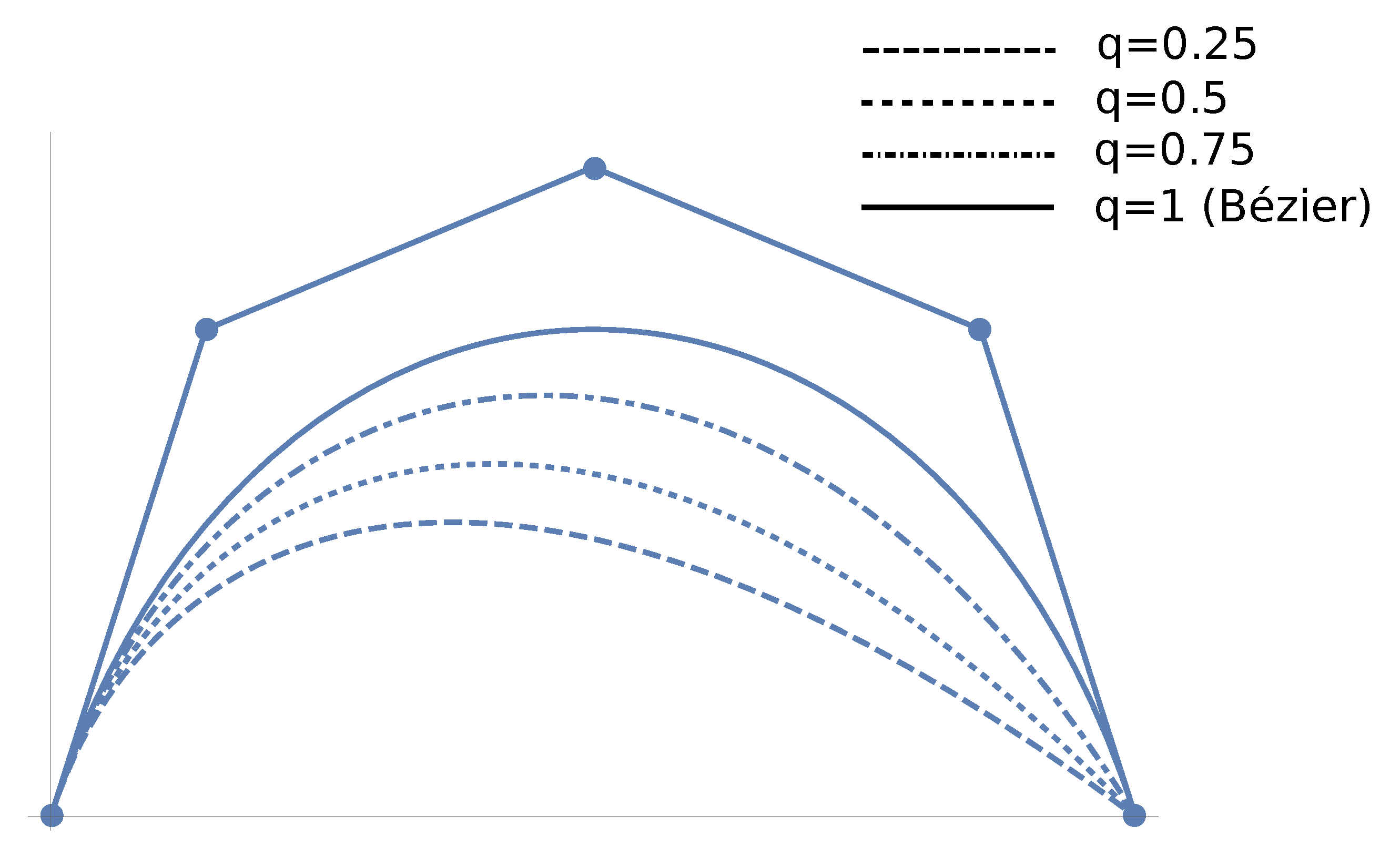
Figure 1 illustrates the boundary tangent property of q-Bernstein bases. We can observe that the theoretical results are confirmed: is tangent to all the q-Bézier curves at , whereas is only tangent to the Bézier curve at the other endpoint .
4. Rational q-Bézier Curves
In [8] rational q-Bézier curves were presented as a generalization of rational Bézier curves. Given a sequence of strictly positive weights, a rational q-Bernstein basis was defined as
and a rational q-Bézier curve as
where ( or 3) are the control points of the curve.
4.1. Properties of Rational q-Bézier Curves
We now summarize some basic properties of rational q-Bézier curves.
- The functions form a partition of unity:
- The functions are nonnegative: for all .
- Affine invariance.
- Endpoint interpolation property: This is a consequence of the identities
- Invariance under barycentric combinations:
- The rational functions form a normalized totally positive basis of the corresponding space of functions since any collocation matrix of this system of functions can be expressed as the product of three totally positive matrices and so it is totally positive. In fact, if we consider a collocation matrix of the system (5), it can be expressed as the product of the corresponding collocation matrix of the system premultiplied and post multiplied by diagonal matrices with positive diagonal entries.
- Rational q-Bézier curves satisfy the variation diminishing property: the rational q-Bézier curve has no more intersections with any line than its control polygon. This property is a consequence of the previous one.
4.2. q-Casteljau Algorithms for Rational q-Bézier Curves
In Algorithm 2.1 of [8] an algorithm for the evaluation of rational q-Bézier curves was also presented. We call it Algorithm 3.
| Algorithm 3 Evaluation of a rational q-Bézier curve |
|
Algorithm 3 arose as a generalization of Algorithm 1 for rational q-Bézier curves. In particular, in [8] the following result was provided.
Theorem 3.
Each intermediate point of Algorithm 3 can be expressed as
Analogously, we can generalize Algorithm 2 obtaining Algorithm 4.
| Algorithm 4 Evaluation of a rational q-Bézier curve |
|
We can observe that Algorithm 4 is an algorithm formed by steps in barycentric form in contrast to Algorithm 3. The following result relates both algorithms.
Theorem 4.
The intermediate values , , and of Algorithms 3 and 4 satisfy
Proof.
Let us prove it by induction on . For we have by Algortihm 4
From the previous expression, by Algorithm 3 and taking into account that we have
that is, the first equation in (7) for . Again by Algortihm 4 for we have
Substituting (8) in the previous formula, by Algorithm 3 and taking into account that and we deduce that
that is, the second equation in (7) for . Now let us assume that formulas in (7) hold for some and let us prove them for . For we have, by Algorithm 4, that
By the induction hypothesis we have that . Applying this fact in the previous formula we have
and, by Algorithm 3, we conclude
that is, the first formula in (7) for . Again by Algortihm 4 for we have
Substituting (9) in the previous formula, taking into account that and and by Algorithm 3 we deduce that
that is, the second equation in (7) for and the theorem holds. □
As a consequence of the previous theorem and Theorem 3, the following result follows.
Corollary 3.
Each intermediate point of Algorithm 4 can be expressed as
In Theorem 3.2 of [8] a result on subdivision of rational q-Bézier curves was stated. So, taking into account that result and (7) we have the following result.
Theorem 5.
Let be a rational q-Bézier curve of degree n given by (6) and let . Then the part of the curve that corresponds to the interval denoted by is given by
where quantities and , and and are computed from Algorithm 3 and Algorithm 4, respectively.
4.3. Boundary Tangent Property for Rational q-Bézier Curves
At the beginning of this section, it was recalled that rational q-Bernstein bases satisfy the endpoint interpolation property. Now let us analyze the boundary tangent property. The following result provides the derivatives of a rational q-Bézier curve at the endpoints.
Proposition 2.
Given the rational q-Bézier curve defined by (6) we have
Proof.
Differentiating (6) we get
Evaluating the previous expression at and and applying Proposition 1 and that
the result follows. □
Analogously to the nonrational case we can derive the following result.
Corollary 4.
The rational q-Bernstein basis satisfies the boundary tangent property if and only if , that is, if and only if it is the corresponding rational Bernstein basis.
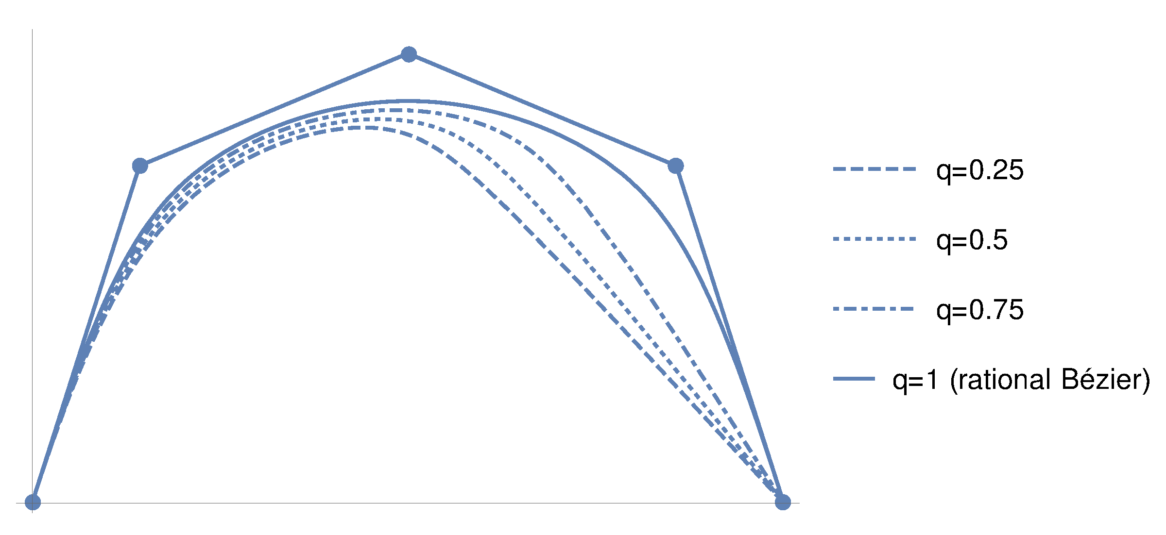
Figure 2 illustrates the boundary tangent property of rational q-Bernstein bases. For the example we have considered the same control points as in the example illustrating the boundary tangent property of q-Bernstein bases with weigths . As in that case, we can observe that the theoretical results are confirmed: is tangent to all the rational q-Bézier curves at , whereas is only tangent to the rational Bézier curve at the other endpoint .
4.4. Degree Elevation of Rational q-Bézier Curves
At the end of Section 3 in [8] it was shown briefly how to elevate by 1 the degree of rational q-Bézier curves. In the following result this procedure is generalized.
Theorem 6.
Let be the rational q-Bézier curve (6) with a sequence of control points in or and a sequence of strictly positive weights. Then
where, for ,
for , and with and for .
Proof.
Denoting by
with for , we have . Applying Theorem 2 and Remark 1 to both and we deduce that
where,
for and , with and for . Then, taking the result follows. □
Example 1.
We have considered the rational q-Bézier curve given by (6) for , , weigths and control points , , , and . Then, applying the degree elevation method for rational q-Bézier curves given in Theorem 6 for we obtain the rational q-Bézier curve given by (11) with weights and control points , , , , , , and . Figure 3 illustrates this particular example of the degree elevation of rational q-Bézier curves. The polygon with dashed line corresponds to the control polygon of the original curve, whereas the other polygon corresponds to the control polygon obtained after of the degree elevation process.
5. Rational q-Bézier Surfaces
Given a matrix of positive weights , a matrix of control points in and , we define the rational q-Bézier surface
Now let us consider the evaluation of q-Bézier rational surfaces. The rational q-Bézier surface in (12) can be written as
Taking into account the previous expression of a rational q-Bézier surface, this can be evaluated by computing the evaluation of the q-Bézier curves, rational and nonrational,
for , and, finally, by computing the evaluation of the following rational q-Bézier curve:
The evaluation of all these functions can be performed by either Algorithm 3 or Algorithm 4, obtaining Algorithm 5 and Algorithm 6, respectively.
| Algorithm 5 Evaluation of a rational q-Bézier surface |
|
| Algorithm 6 Evaluation of a rational q-Bézier surface |
|
Taking for all and in (12) a tensor product q-Bézier surface is obtained. For this particular case, Algorithms 5 and 6 are two evaluation algorithms alternative to the algorithm for the evaluation of tensor product q-Bézier surfaces proposed in [12].
As a consequence of the subdivision properties of Algorithms 3 and 4 in Theorem 5, we deduce the following subdivision properties for Algorithms 5 and 6.
Theorem 7.
Let a rational q-Bézier surface given by (12) and let . Then the part of the surface that corresponds to , denoted by , is given by
where quantities and , and and are computed from Algorithm 5 and Algorithm 6, respectively.
6. Conclusions
In this paper, it is shown that many properties and efficient algorithms for Bézier curves and surfaces can be extended to q-Bézier curves and surfaces, showing some differences. The existence of evaluation algorithms formed by steps in barycentric form for the rational q-Bézier curves and surfaces is also proved. Therefore, q-Bézier curves and surfaces can be very useful, sharing many nice properties with Bézier curves and surfaces and, in addition, providing greater flexibility. We also conclude that there are some limitations with respect to Bézier curves and surfaces. For instance, with the geometric boundary tangent property. Finally, we can use for rational q-Bézier curves and surfaces algorithms with many nice properties of rational Bézier curves and surfaces.
Author Contributions
All authors contributed equally in this research paper. All authors have read and agreed to the published version of the manuscript.
Funding
This research was partially funded by the Spanish research grant PGC2018- 096321-B-I00 (MCIU/AEI), by Gobierno de Aragón (E41-17R) and Feder 2014-2020 “Construyendo Europa desde Aragón”.
Conflicts of Interest
The authors declare no conflict of interest. The funders had no role in the design of the study; in the collection, analyses, or interpretation of data; in the writing of the manuscript, or in the decision to publish the results.
Abbreviations
The following abbreviations are used in this manuscript:
| CAGD | Computer-Aided Geometric Design |
References
- Phillips, G.M. Bernstein polynomials based on the q-integers. Ann. Numer. Math. 1997, 4, 511–518. [Google Scholar]
- Goldman, R.; Simeonov, P. Two essential properties of (q,h)-Bernstein-Bézier curves. Appl. Numer. Math. 2015, 96, 82–93. [Google Scholar] [CrossRef]
- Goldman, R.; Simeonov, P.; Simsek, Y. Generating functions for the q-Bernstein bases. SIAM J. Discrete Math. 2014, 28, 1009–1025. [Google Scholar] [CrossRef]
- Carnicer, J.M.; Peña, J.M. Shape preserving representations and optimality of the Bernstein basis. Adv. Comput. Math. 1993, 1, 173–196. [Google Scholar] [CrossRef]
- Carnicer, J.M.; Peña, J.M. Totally positive bases for shape preserving curve design and optimality of B-splines. Comput. Aided Geom. Des. 1994, 11, 633–654. [Google Scholar] [CrossRef]
- Kac, V.; Cheung, P. Quantum Calculus, Universitext; Springer: New York, NY, USA, 2002. [Google Scholar]
- Delgado, J.; Peña, J.M. Accurate computations with collocation matrices of q-Bernstein polynomials. SIAM J. Matrix Anal. Appl. 2015, 36, 880–893. [Google Scholar] [CrossRef]
- Dişibüyük, Ç.; Oruç, H. A generalization of rational Bernstein-Bézier curves. BIT Numer. Math. 2007, 47, 313–323. [Google Scholar] [CrossRef]
- Simeonov, P.; Zafiris, V.; Goldman, R. q-Blossoming A new approach to algorithms and identities for q-Bernstein bases and q-Bézier curves. J. Approx. Theory 2012, 164, 77–104. [Google Scholar] [CrossRef] [Green Version]
- Oruç, H.; Phillips, G.M. q-Bernstein polynomials and Bézier curves. J. Comput. Appl. Math. 2003, 151, 1–12. [Google Scholar] [CrossRef] [Green Version]
- Phillips, G.M. A de Casteljau algorithm for generalized Bernstein polynomials. BIT 1996, 36, 232–236. [Google Scholar] [CrossRef]
- Dişibüyük, Ç.; Oruç, H. Tensor product q-Bernstein polynomials. BIT Numer. Math. 2008, 48, 689–700. [Google Scholar]
Figure 1.
Boundary tangent property of q-Bernstein bases.

Figure 2.
Boundary tangent property of rational q-Bernstein bases

Figure 3.
Degree elevation of rational q-Bézier curves.

© 2020 by the authors. Licensee MDPI, Basel, Switzerland. This article is an open access article distributed under the terms and conditions of the Creative Commons Attribution (CC BY) license (http://creativecommons.org/licenses/by/4.0/).
Share and Cite
MDPI and ACS Style
Delgado, J.; Peña, J.M. Geometric Properties and Algorithms for Rational q-Bézier Curves and Surfaces. Mathematics 2020, 8, 541. https://0-doi-org.brum.beds.ac.uk/10.3390/math8040541
AMA Style
Delgado J, Peña JM. Geometric Properties and Algorithms for Rational q-Bézier Curves and Surfaces. Mathematics. 2020; 8(4):541. https://0-doi-org.brum.beds.ac.uk/10.3390/math8040541
Chicago/Turabian StyleDelgado, Jorge, and J. M. Peña. 2020. "Geometric Properties and Algorithms for Rational q-Bézier Curves and Surfaces" Mathematics 8, no. 4: 541. https://0-doi-org.brum.beds.ac.uk/10.3390/math8040541
Note that from the first issue of 2016, this journal uses article numbers instead of page numbers. See further details here.