A Comparative Study of Swarm Intelligence Algorithms for UCAV Path-Planning Problems


1
School of Artificial Intelligence, Jilin University, Changchun 130012, China
2
School of Computer Science and Technology, Northeast Normal University, Changchun 130117, China
*
Authors to whom correspondence should be addressed.
†
Current address: School of Artificial Intelligence, Jilin University, Changchun 130012, China.
‡
These authors contributed equally to this work.
Mathematics 2021, 9(2), 171; https://0-doi-org.brum.beds.ac.uk/10.3390/math9020171
Submission received: 11 November 2020
/
Revised: 23 December 2020
/
Accepted: 12 January 2021
/
Published: 15 January 2021
(This article belongs to the Special Issue Multivariable Optimization by Intelligent and Numerical Modelling and Simulation)
Abstract
:Path-planning for uninhabited combat air vehicles (UCAV) is a typically complicated global optimization problem. It seeks a superior flight path in a complex battlefield environment, taking into various constraints. Many swarm intelligence (SI) algorithms have recently gained remarkable attention due to their capability to address complex optimization problems. However, different SI algorithms present various performances for UCAV path-planning since each algorithm has its own strengths and weaknesses. Therefore, this study provides an overview of different SI algorithms for UCAV path-planning research. In the experiment, twelve algorithms that published in major journals and conference proceedings are surveyed and then applied to UCAV path-planning. Moreover, to demonstrate the performance of different algorithms in further, we design different scales of problem cases for those comparative algorithms. The experimental results show that UCAV can find the safe path to avoid the threats efficiently based on most SI algorithms. In particular, the Spider Monkey Optimization is more effective and robust than other algorithms in handling the UCAV path-planning problem. The analysis from different perspectives contributes to highlight trends and open issues in the field of UCAVs.
1. Introduction
Path-planning for uninhabited combat air vehicle (UCAV) task is one of the key problems in the UCAV system, which aims to find a path with the shortest distance while ensuring safety. A safe path denotes that the aircraft can reach the destination without hitting an obstacle or being detected by radar. The development of the UCAV system has been receiving increasing attention since it can accomplish difficult tasks in a complicated environment. In the previous study, many models have been taken to simulate the intelligent behavior that the aircraft might find a suitable path automatically [1,2]. Under that model, a series of methods to produce an optimal path have been proposed [3]. The angle, velocity, and height and many other factors should be involved in those methods. In [4], You et al., proposed a three-dimensional (3D) path-planning approach based on the situational space to provide the tactical requirements of UCAVs for tracking targets and avoiding collisions. In [5], a two-stage method for solving the terrain-following (TF)/terrain-avoidance (TA) path-planning problem for UCAV is presented, where the first stage of planning takes an optimization approach for generating a 2D path on a horizontal plane with no collision with the terrain, and in the second stage of planning, an optimal control approach is adopted to generate a 3D flyable path for the UCAV that is as close as possible to the terrain. In [6], the online collaborative path-planning method based on dynamic task allocation is proposed. However, they always suffer from the weakness of UCAVs’ real-time response capability due to the high complexity.
Swarm intelligence algorithms with a new simple model for the path-planning task have been widely proposed to overcome the complexity. For example, Pehlivanoglu et al. [7] proposed a multi-frequency vibrational genetic algorithm to address the path-planning of UCAV. A new mutation application strategy and diversity variety are designed. In [8], Zhang et al. used the grey wolf optimizer to deal with UCAV path-planning using the traditional cost function model. In [9], an improved bat algorithm is employed for three-dimensional UCAV path-planning by Wang et al., in which BA is combined with differential evolution. Recently, Yi et al. proposed a quantum-inspired monarch butterfly optimisation [10] for the UCAV path-planning navigation problem. The worst individuals are updated by quantum operators to prevent being trapped in local optima, enhancing the search efficiency. In [11], Pan et al. proposed CIJADE to deal with the UCAV path-planning problem. It is a hybrid differential evolution algorithm that taking advantages of the modified CIPDE (MCIPDE) and modified JADE (MJADE) with great searchability. Moreover, Huang et al. [12] applied the SI algorithms to multi-model cooperative task assignment and path-planning of multiple UCAV formation, where the task assignment model of the UCAV formation is developed based on the flight characteristics of the UCAV formation and constraints in the battlefield. Dewangan et al. [13] applied the grey wolf optimization to the multi-UCAV path-planning problem in the three-dimensional environment. It expresses the trajectory of UCAV in the real 3D battlefield more vividly. Even more, in [14], Paszkiel et al. discussed the use of brain–computer interface to control unmanned aerial vehicles. A novel method is proposed to control the UCAV with a microcomputer connected with the human brain.
All those SI algorithms in solving such complex problems have common specific characteristics [15], such as sharing information between individuals to enhance the population quality [16,17]. However, each swarm intelligence algorithm has its own strengths and weaknesses [18]; different swarm intelligence algorithms provide various performance for cases with different UCAV scales. It is hardly believed that a single swarm intelligence algorithm can address all complex problems without detailed analysis from multiple perspectives [19]. Therefore, we provide a comprehensive comparison by studying similarities and differences between the twelve SI algorithms in UCAV path-planning. Particularly, a recently swarm intelligence algorithm called Spider monkey optimization [20] is applied to address the UCAV path-planning under the self-organization and division of labor. Moreover, we design thirty UCAV path-planning cases with different scales to demonstrate the performance of each algorithm. The effectiveness and robustness of each algorithm are further analyzed from different perspectives on those thirty different cases. Experimental results demonstrate that Spider monkey optimization can provide better performance over other state-of-the-art algorithms with good robustness.
2. Problem Formulation
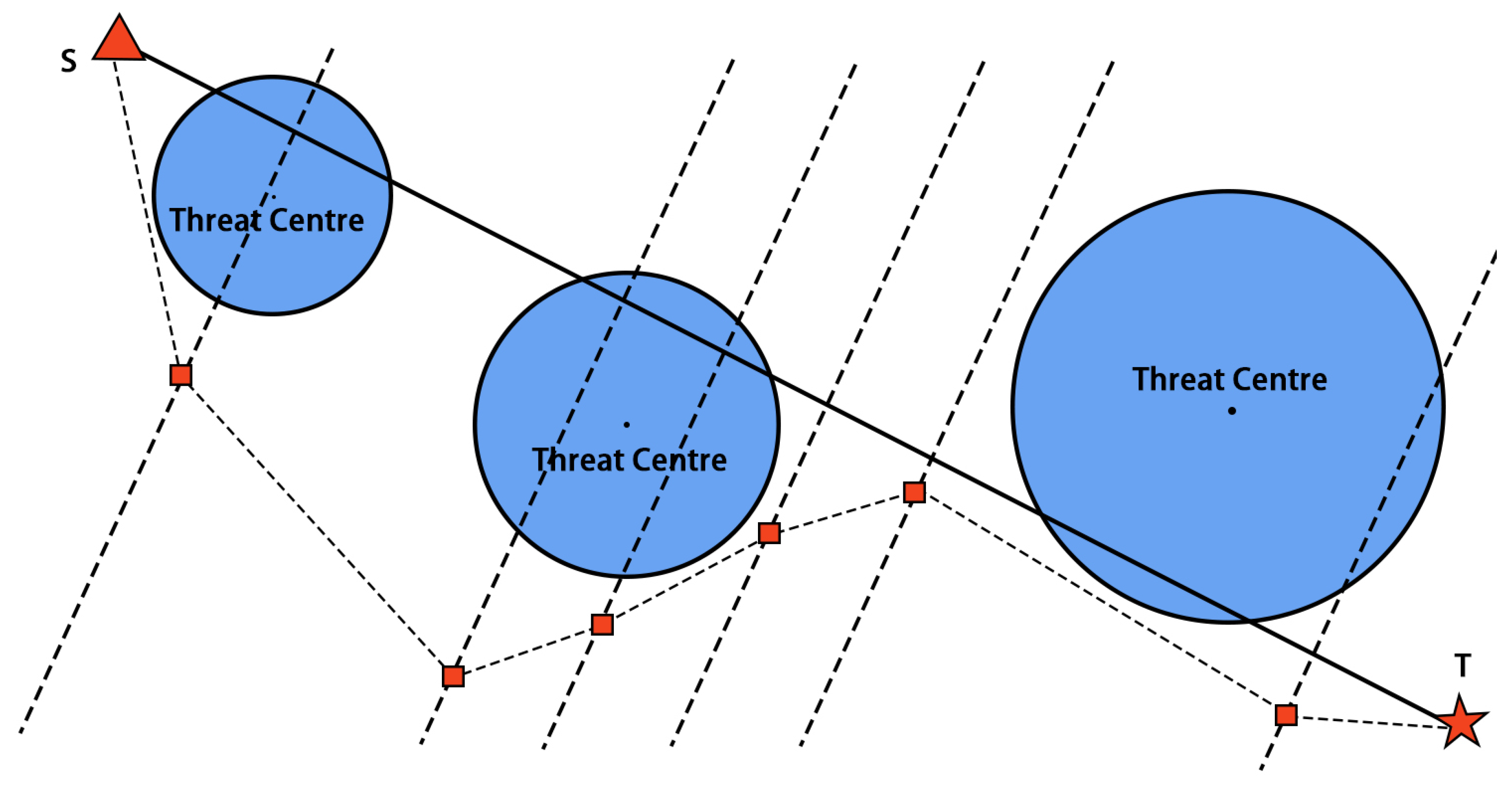
Path-planning of Uninhabited Combat Air Vehicles (UCAV) is a numerical problem where emergencies should be considered. It aims to arrive at the destination safely by finding a superior path to avoid any threat, which accounts for artificial threats and natural constraints. The UCAV path-planning problem is usually represented by the classic 2D model, as shown in Figure 1. As depicted in this figure, we can clearly see that a path can be found to link up the starting point and the terminal end, and threats presented in circles are avoided. In the first, a segment that directly connected the starting and terminal point is drawn, then it is divided into equal parts by D perpendicular lines. After that, these D lines are taken as a new axis, onto which a series of points are set and connected one by one to form a path. Under this model, the whole path is divided into steps represented by a vector , where is the dimension of the solution vector, and it indicates a discrete position of each step in the vertical axis. The way of representing the path (a solution) is using a vector in the form of . For example, considering the coordinate is the starting point and is the terminal point, then the distance between the starting and the terminal point is T. A path with D steps can be performed by that vector , thus the coordinate of the first step is , the coordinate of the second step is , and so on. With all the steps linked up, the whole path can be formed. Since the paths can not be away from the battle area, the restriction of each solution path on each case can be set manually related to the size of the battlefield.
To measure those paths, a probability density model is formulated as Equation (1). Unlike the traditional cost function model, there is no distinct boundary where the damage risk remains zero. As distance increases, the probability of being attacked by a threat regularly decreases, but it’s going to in no way be zero. indicates the distance between the step and the threat center, is a parameter to control the shape of the density function:
Indeed, the UCAV speed and the entire distance of a path should be taken into consideration. Simplify, it is assumed that the UCAV maintains a constant speed, and then the fuel consumption corresponds with the total distance of the path. Under that, the complete cost function can be described as:
where is the weighting factor ranging in [0,1], and is set to 0.5. is the length of the segment . refers to the length of the whole flight path, and is the length of the step of the solution. Since each step is connected directly as a segment, can be calculated by the pythagorean theorem:
where and are the horizontal and vertical projection of each step. In this study, Equation (2) is adopted as the objective function, a solution with smaller objective value denotes a path with better quality.
3. Methodology
Many computational methods have been proposed for addressing path-planning of UCAV [1,2,3]. Unfortunately, those computational methods often suffer from numerical instability and premature convergence due to their inefficient search capabilities and high complexity. Recently, swarm intelligence (SI) algorithms have been proven to be a competitive approach to deal with such difficult problems [21,22,23,24]. Generally speaking, SI algorithms are inspired by nature or population-based. They are heuristic methods that exchange information among the entire population iteratively. However, each swarm intelligence algorithm has its own strengths and weaknesses; different swarm intelligence algorithms provide various performance on different UCAV scales due to their algorithmic parameters based on the problem characteristics. To demonstrate the performance of different swarm intelligence algorithms in the UCAV path-planning problem, a comparison of 12 SI algorithms is studied. The mechanical characteristics and parameters of each algorithm for the UCAV path-planning problem are listed in Table 1. Moreover, four algorithms including Grey Wolf Optimizer, Firefly Algorithm, Harmony Search, Spider Monkey Optimization are introduced.
3.1. Grey Wolf Optimizer
Grey wolf optimizer was inspired by the special predatory behavior of grey wolves, which has a hierarchy system in the population and encircles their prey in a clear labor division. The leaders are called the alphas. They are mostly responsible for making decisions about hunting, sleeping place and so on. The second level in the hierarchy is beta, which helps the alpha make decisions, like the military adviser. The lowest level, omega, plays the role of the scapegoat. They submit to all the other dominant wolves. If a wolf is not an alpha, beta or omega, it’s called a delta. Delta wolves have to submit to alphas and betas, but they dominate the omega.
In GWO, it considers the best solution as the alpha (), then the second and the third best solutions are named beta () and delta () respectively. The rest individuals in the population are omegas (), which are guided by , and during the hunting process. In each iteration, each individual is updated by:
where t indicates the current iteration. and are coefficient vectors, are the three leader wolves’ vectors, and X is the position vector of a grey wolf. and are calculated as follows:
where a is linearly decreased from 2 to 0 over iterations, and are random vectors in [0,1]. Equation (4) mathematically models the behaviour of encircling and hunting.
3.2. Firefly Algorithm
Firefly algorithm is an effective swarm intelligence method based on the behavior of fireflies that brighter fireflies would attract other fireflies. As observed from the natural world, a group of fireflies would always fly towards the brightest one. Brightness measures the quality of fireflies, therefore the brightness or light intensity in the algorithm can be represented by the objective function. To simplify, all fireflies are set unisex so that one firefly is attracted to other fireflies regardless of their sex. Attractiveness is related to their distance, which can be calculated by the equation below:
where is to control the size of attractiveness, and is set to 1 for the UCAV path-planning problem. is the consumption factor and set to 0.01. is the cartesian distance of two fireflies. For firefly i, it checks every firefly in the whole group. If it finds a brighter or better firefly j, firefly i is attracted and moves towards firefly j with a random walk in all dimensions by:
where is the randomization walk for local searching. is a coefficient decreasing with iterations, is a random vector with D dimensions ranging in [0,1] and L is the difference between the upper and lower bounds.
3.3. Harmony Search
Harmony search algorithm is a heuristic algorithm derived from an artificial phenomenon found in music performance to search for better harmony. A harmony is composed of many different kinds of instruments, and only the same instruments can adjust from each other. For instance, the piano part of harmony is subpar, and the piano part can only improve itself from the experience of pianos in other similar harmonies. Aesthetic estimation measures the quality of a harmony. Practice by practice makes a fantastic harmony, just as the values for better objective function evaluation can be improved iteration by iteration.
In Harmony Search (HS), a new harmony is improvised from the population in each iteration. The way each dimension updates depends on a probability . If a random number is smaller than , the certain dimension of a randomly selected harmony is used for the newly generated harmony. Or it is generated randomly. For example, suppose there are a total of ten vectors in the population. For the dimension of the new harmony, the third vector in the population is selected randomly for the new harmony. After that, a further adjustment is executed by probability . If , the adjustment proceeds as equation below:
where is the difference between the upper and lower bounds. Or no change is made. This step guarantees the global search ability of HS. If the newly created harmony is better than the worst harmony in the population, it will replace the worst one. An overview of HS is summarized in [35].
3.4. Spider Monkey Optimization
Spider Monkey Optimization (SMO) is a novel optimization algorithm that is inspired by the fission-fusion social system of the spider monkey. These smart creatures have an impressive mechanism to find the best food source: the leader of the population, usually a female monkey, leads the group. However, if she can’t find a sufficient target for the whole group, she divides the whole group into smaller subgroups that explore respectively. Each subgroup has a leader. Communications are made among the individuals in every subgroup and with other subgroup individuals as follows:
where is a random number in the range [0,1] and is the local leader in the subgroup. is a randomly selected individual in the entire group.
If the global leader does not update herself in a certain number of iterations, namely , the whole group breaks into certain numbers of subgroups. If a local leader remains the same for a certain number of iterations, namely , the subgroup is re-generated randomly or simply attracted by the global leader by:
where is the global leader. The number of subgroups has a limitation . If is reached, all the subgroups reunion into an entire group.
3.5. Proposed Framework for UCAV Path-Planning Problem
In this study, the UCAV path-planning task is a numerical problem, where a superior path with the lowest objective value needs to be found. It has been proven that SI methods are effective approaches to deal with optimal problems. First, the population composed of some individuals is randomly initialized, and the probability density model evaluates each individual. Then the process of different search strategies proceeds to optimize the population after the iterations. The SMO algorithm is used to address the UCAV path-planning problem.
3.5.1. Initialization
In Section 2, the 2D model transforms the battlefield to the top view of the map, and a path divided by several steps is linked up from the starting point and the terminal ending. Thus, the path can be represented by a vector , where and D denotes the number of steps in each path, and indicates the position of the step of the individual in the whole population.
The population consists of a certain number of individuals (N). The initial population covers the entire battlefield as much as possible by randomizing the paths within the upper and lower bounds and of the map. Therefore, the population is initialized as follows:
3.5.2. Local Leader Phase
After initialization, each path in every subgroup updates its current position based on the experience of its local leader and local group paths in local lea, by:
where is the step of the local leader under the current subgroup. is a randomly chosen path among the subgroup and , and is a random number ranging in [a,b] that obeys uniform distribution. Algorithm 1 summarised the local leader phase of SMO for UCAV path-planning problem. is the perturbation rate which controls the frequency of perturbation in the current position. After that, the objective value is calculated by the probability density model, and the lower the objective value of a path is, the more qualified the path is. According to the greedy rule, if the newly updated path is better than the old one, the path is replaced with the new one.
| Algorithm 1 Local leader phase |
|
3.5.3. Global Leader Phase
After the local leader phase, all the paths update their positions using the experience of the global leader and local group members by . The global leader phase is summarized in Algorithm 2, from which we can see that the better paths with higher are more likely further to update themselves. If , the evolutionary search strategy proceeds and can be described as follows:
where is the step of the global leader and is a randomly chosen step. The could be calculated by:
where is the value of the path. can be calculated by anyway related to the objective value of the paths.
| Algorithm 2 Global leader phase |
|
Further, the objective of the newly generated path is compared with the old one and the better one is adopted.
3.5.4. Local Leader Decision Phase
In order to prevent stagnation, the local leader decision phase is proposed. The local leader is the best path in the current subgroup, and if any newly updated paths are found better than the local leader, the better path is maintained. If any local leader is not optimized for a threshold called , then all paths in this subgroup update their positions by either rerandom generation or by using combined information from the global leader and the local leader in this group, which depends on the probability . In this way, any paths have chances to move closer to the best path in the whole group, which guarantees the search capability. The local leader decision phase is summarized in Algorithm 3.
| Algorithm 3 Local leader decision phase |
|
3.5.5. Global Leader Decision Phase
The global leader decision phase is another method to prevent stagnation. The global leader is the best path in the entire population; thus, it has the lowest objective value and the smoothest route. Similar to the local leader decision phase, if any newly updated paths are better than the global leader, it will replace the global leader. Therefore, there might be a situation where the global leader is trapped in stagnation. The global leader decision phase is summarised in Algorithm 4. If the global leader is not updated after a certain number of iterations, namely , the global leader divides the population into smaller subgroups, or simply reunion all the subgroups into a single group and start a new round of search, which depends on the current number of subgroups . The global leader decision phase guarantees the ability of local search, which can prevent the path from trapping into local optimum, and that’s the reason why paths provided by SMO are always smoother than others’.
| Algorithm 4 Global leader decision phase |
|
3.5.6. Time Complexity Analysis
In this section, we analyze the time complexity of SMO for addressing UCAV path-planning problem. Each individual in the population needs to be traversed in local leader phase, and N of individuals are further updated, therefore the time complexity is . After that, the population needs to be evaluated with all probability density model threats, as shown in Equation (2). The time complexity of the objective function evaluation is , where K is the number of threats. To sum up, the overall time complexity is , where t is the number of iterations, N is the population size, D is the number of dimensions.
4. Experimental Results and Discussion
Twelve algorithms are used for comparison in this work, including artificial bee colony algorithm (ABC), bat algorithm (BA), cuckoo search (CS), differential evolution (DE), firefly algorithm (FA), monarch butterfly optimization with greedy strategy (GCMBO), grey wolf optimization (GWO), harmony search (HS), moth search algorithm (MSA), particle swarm optimization (PSO), spider monkey optimization (SMO), and whale optimization algorithm (WOA).
4.1. Cases Design
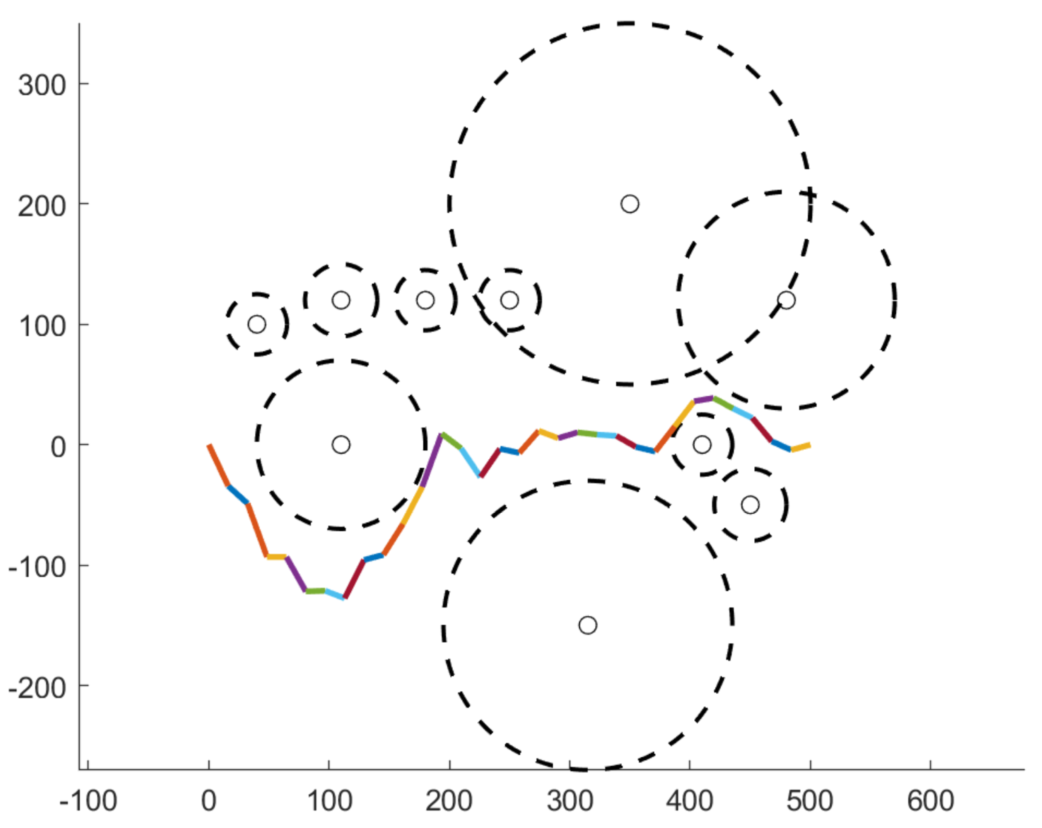
We have adopted 30 different cases including 10 small-scale (D = 20), 10 medium-scale (D = 30), and 10 large-scale cases (D = 60). Each case contains a certain number of threats represented by circles, as shown in Figure 2, and an outstanding path should avoid the threats and arrives at the terminal ending safely.
Moreover, we intentionally design some cases where some of the threats in the map are at an intersection to demonstrate the robustness of our proposed model.
4.2. Parameter Setting
The comparisons are made for thirty cases with the probability density model to optimize the objective function. For all swarm intelligence algorithms, the number of population N is set to 20 for small-scale and 30 for medium-scale and large-scale cases. Other parameters of different SI algorithms are listed in Table 1. In SMO, it can be noticed that is the perturbation rate, which controls the frequency of perturbation in the current position. If the value of is too large, the result might be converged after a certain number of iterations. Conversely, if is too small, the results can get converged after a less number of iterations with worse value. Therefore, we selected from . By conducting lots of prior experiments, the best result for SMO is obtained when . Thus we set to 0.375 in SMO. The number of fitness evaluations depends on the operators and the population update model. Different operators of the algorithms can lead to very different numbers of fitness evaluations per iteration. Therefore, the number of fitness evaluations is adopted as the stopping criteria instead of the number of iterations [22]. In our study, we set the . To make statistical analysis, each algorithm runs twenty-five times independently. The average and standard deviation results over 25 independent runs are calculated.
4.3. Performance Comparison on Small-Scale Cases
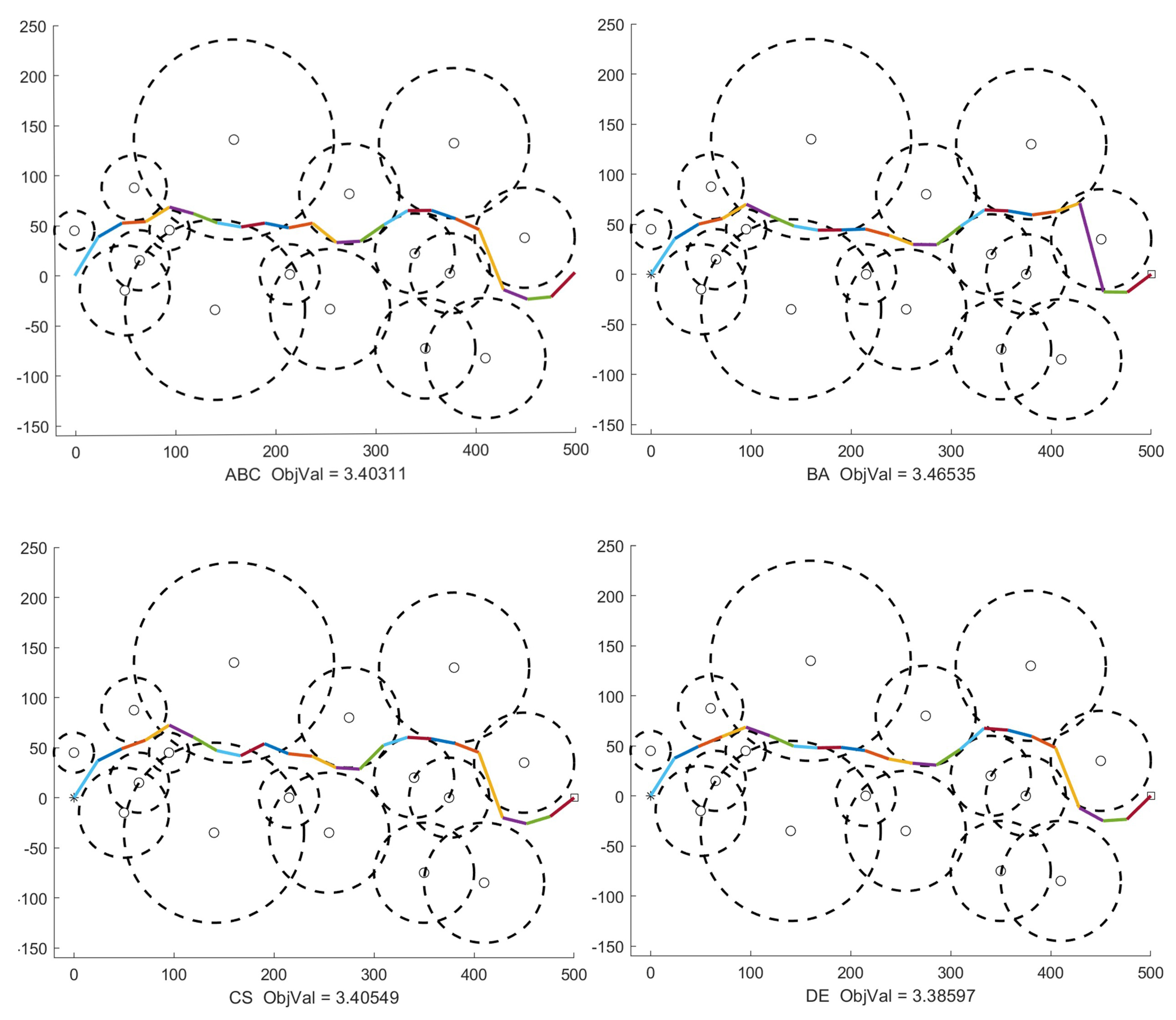
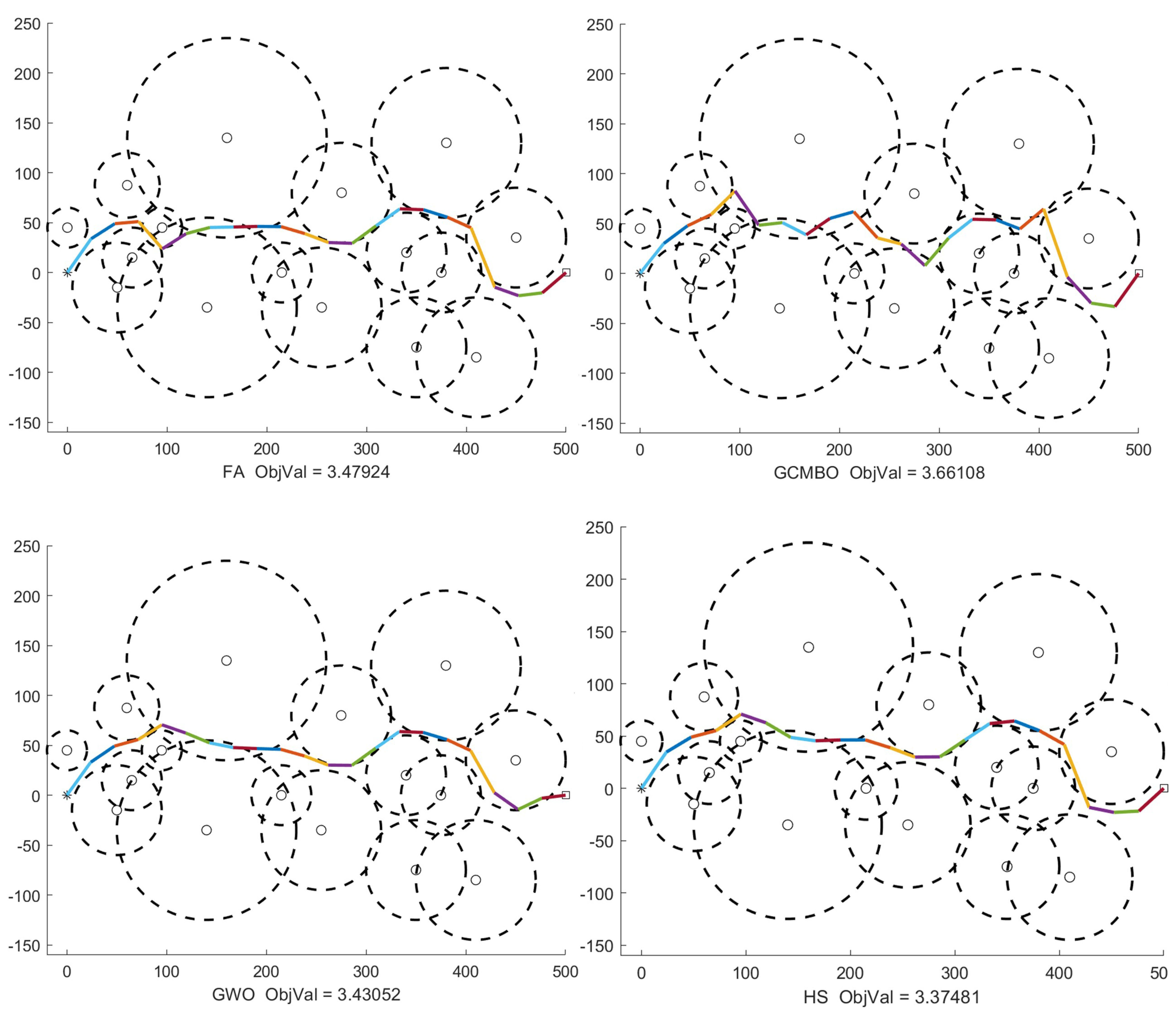
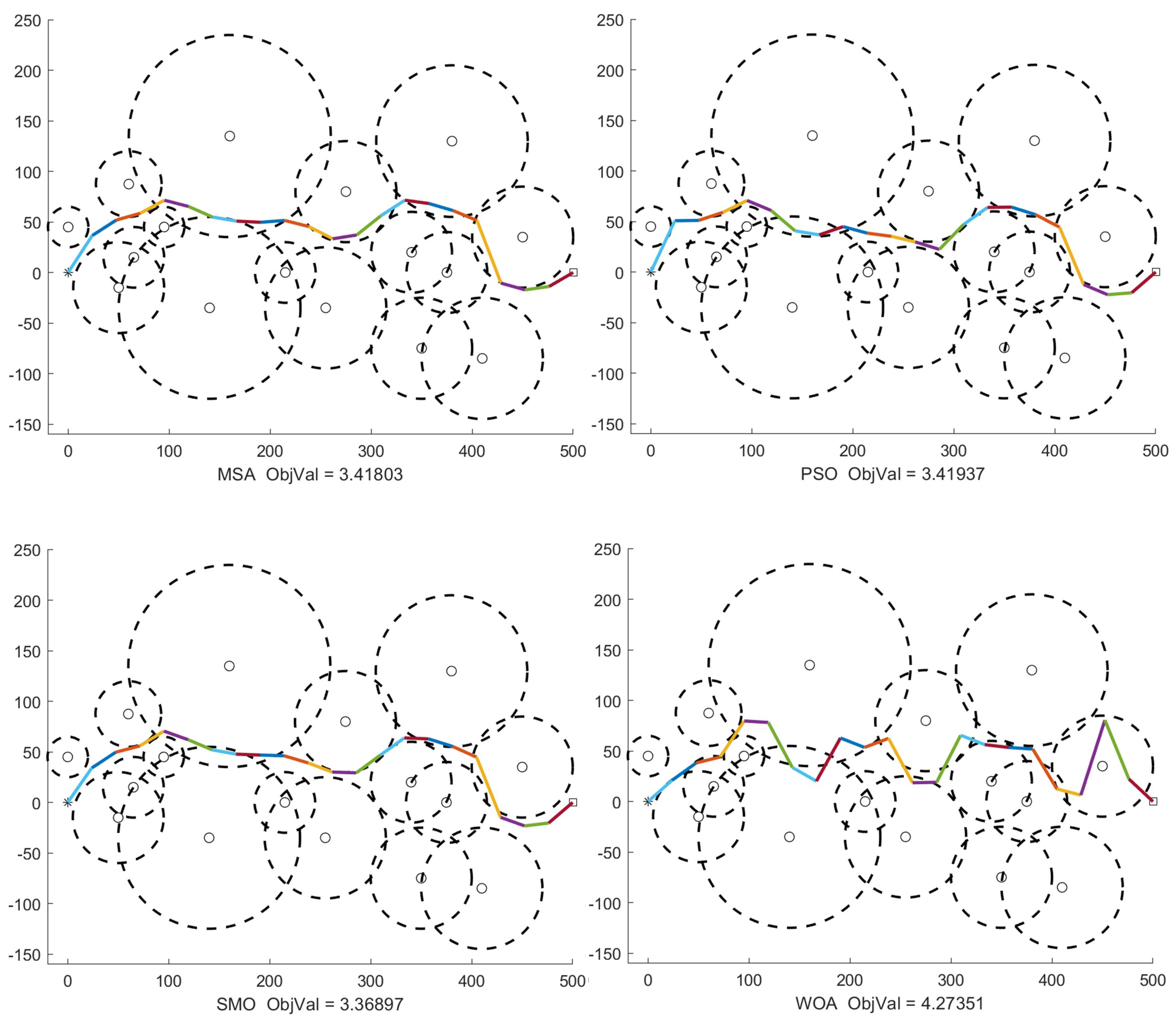
In this section, ten small-scale cases for D = 20 are employed to demonstrate the effectiveness of each SI algorithm for the UCAV path-planning problem. We take Case 8 in those cases for an example to show the best paths provided by each method over 25 independent runs. The comparative performance of each algorithm on Case 8 is visualized in Figure 3, Figure 4 and Figure 5. The horizontal axis is the length of the battlefield and the vertical axis is the width of the battlefield. The unit can be any unit that represents the length. As shown in Figure 3, Figure 4 and Figure 5, it demonstrates that most SI algorithms can successfully avoid the obstacles and reach the terminal ending safely. For each case, the best value, the worst value, average value, and standard deviation are summarized in Table 2. From Table 2, it is observed that SMO can obtain better result (on average, worst) than the other algorithms on all the cases. For Case 2, BA and FA can provide the similar best values with SMO. For Case 3, FA and SMO achieve the similar best values. In particular, SMO shows its strong robustness for four cases including Cases 3, 4, 7, and 8 since its std deviation is zero over multiple runs. For Case 9, HS can reach a slightly smaller std deviation than SMO. However, SMO performs better on best, worst, and average value than HS across 25 times. In terms of those 10 small-scale cases, SMO reaches the best average result for Case 2 and the worst average result for Case1 when multiple runs are made. Moreover, SMO can reach the best value to 1.47449 for Case 2 while WOA can only achieve to 1.73079. Based on those analysis, we can conclude that paths made by SMO have the best performance and the least standard deviation, which reflects that SMO has the best optimization stability for UCAV path-planning problems.
4.4. Performance Comparison on Medium-Scale Cases
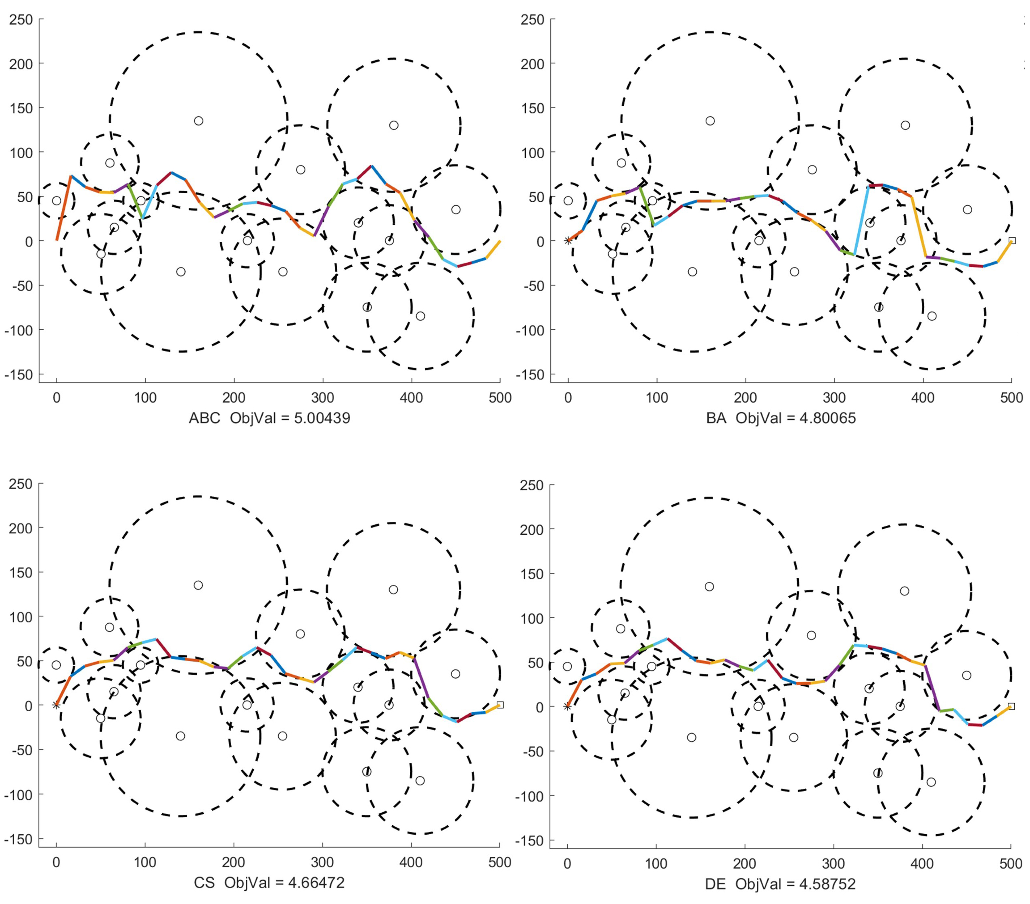
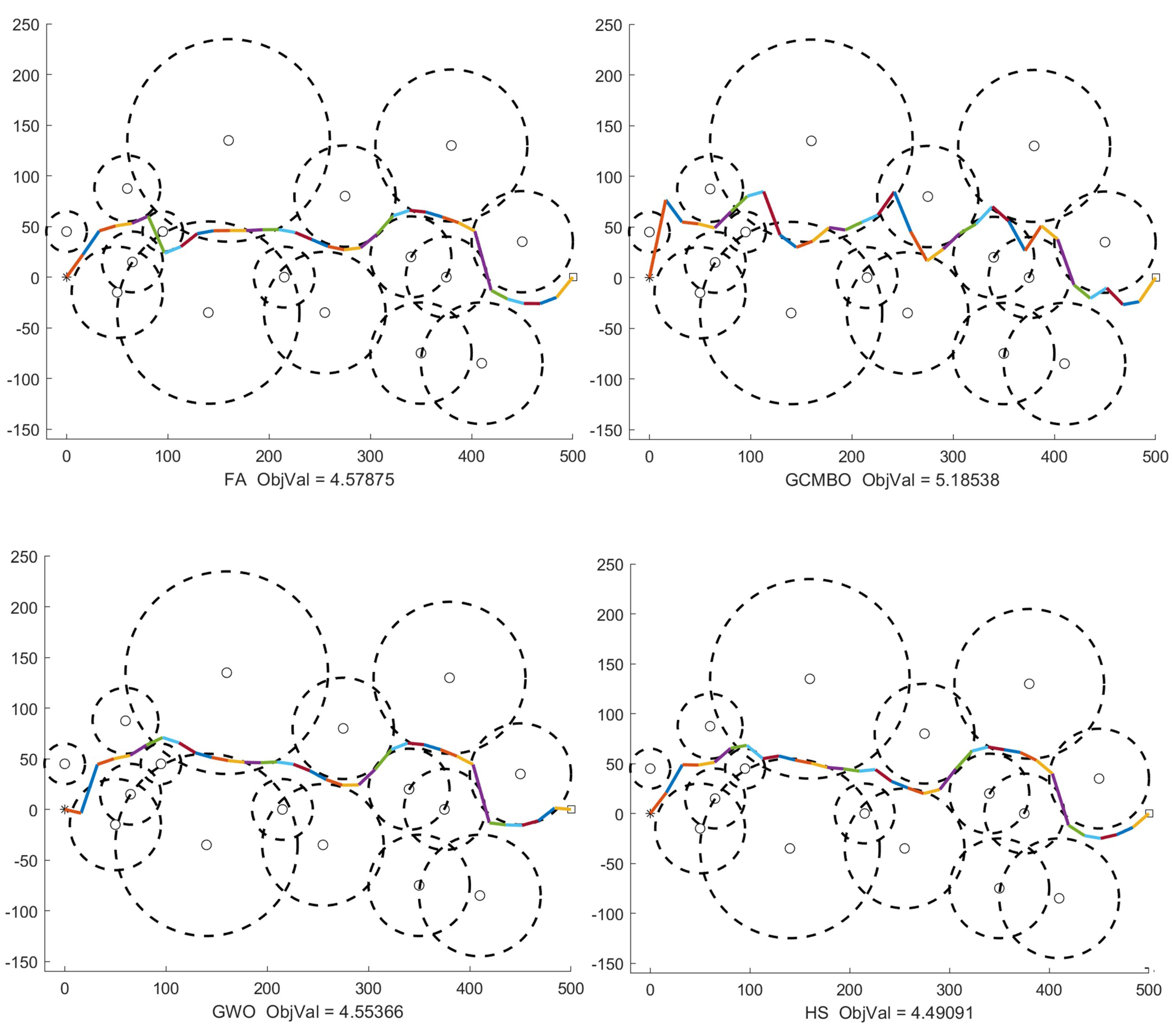
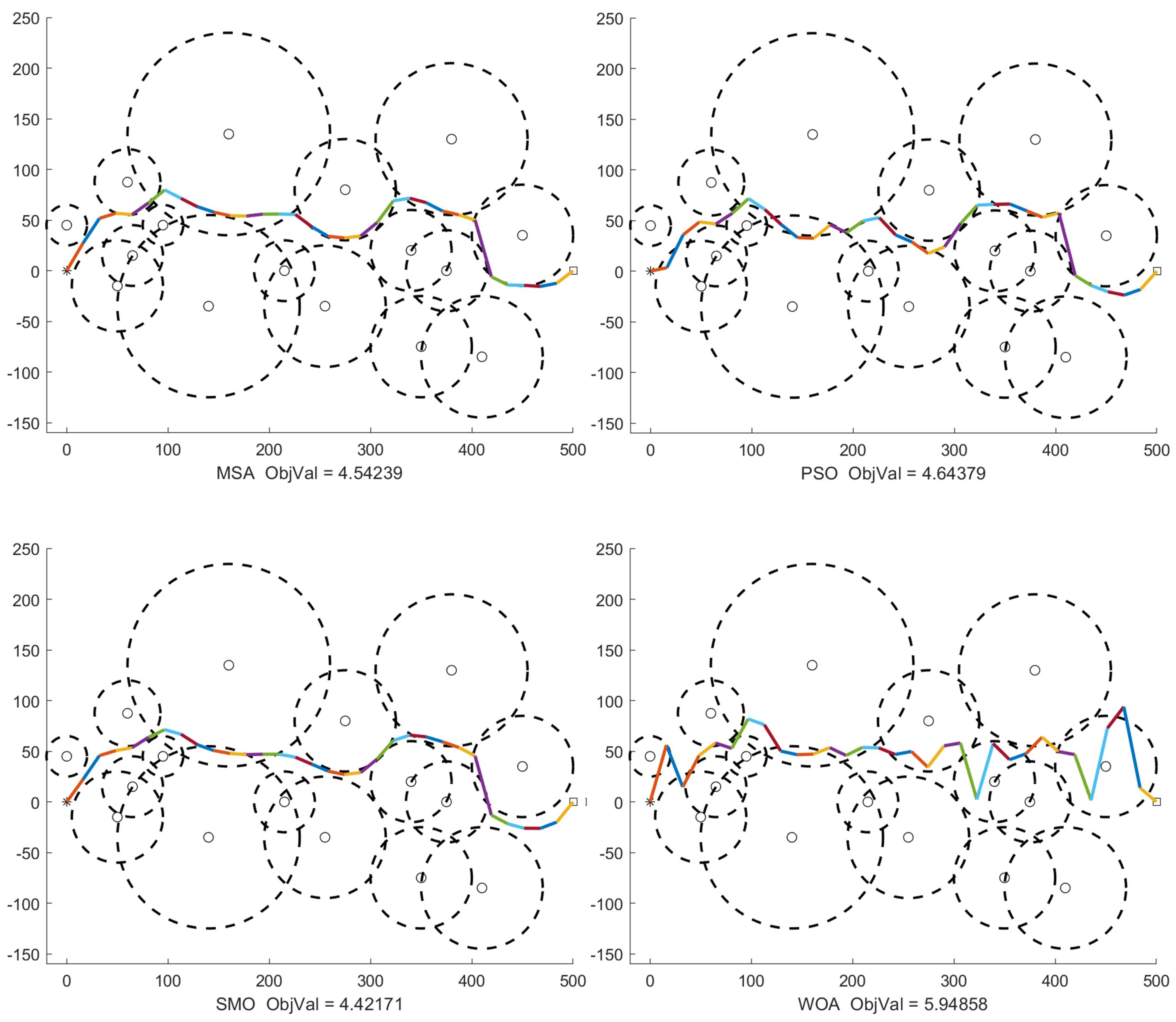
This section is devoted to show the comparative performance of each algorithm on ten medium-scale cases (D = 30). Case 8 of those ten cases is taken as an example to present the best paths gained by each algorithm over 25 runs. The path results are shown in Figure 6, Figure 7 and Figure 8. As depicted in Figure 6, Figure 7 and Figure 8, there is a noticeable difference between each path. ABC, BA, CS, GCMBO, and PSO generate less smooth path than those made by the other algorithms. Some paths of them can be trapped in local optimum. It can be noted that SMO can perform the smoothest path among all the comparative algorithms. To further demonstrate the effectiveness of each algorithm, Table 3 summarizes the cost objective values of each algorithm on each case. From Table 3, we can find that SMO has the best performance while WOA performs the worst. Across all those ten cases, SMO provides the best results on average, best, and worst with the least std deviation. FA can obtain the similar result on Case 3 with SMO. For HS, it achieves the similar std deviation with SMO on Case 6. In terms of Cases 7 and 8, SMO can always produce the best results over 25 times. The average results for Cases 7 and 8 gained by SMO are 4.04452 and 4.42171 respectively while WOA only reaches to 6.41485 and 6.93741 on Cases 7 and 8. It demonstrates that SMO can enhance the performance may due to the division characteristic of SMO. Besides, the minimum and maximum best result are 1.6787 and 5.2963 generated by SMO on Cases 2 and 1 with different threat conditions. In conclusion, it can be summarized that SMO is more effective than other algorithms and suitable for solving the UCAV path-planning problem in medium-scale with high stability.
4.5. Performance Comparison on Large-Scale Problems
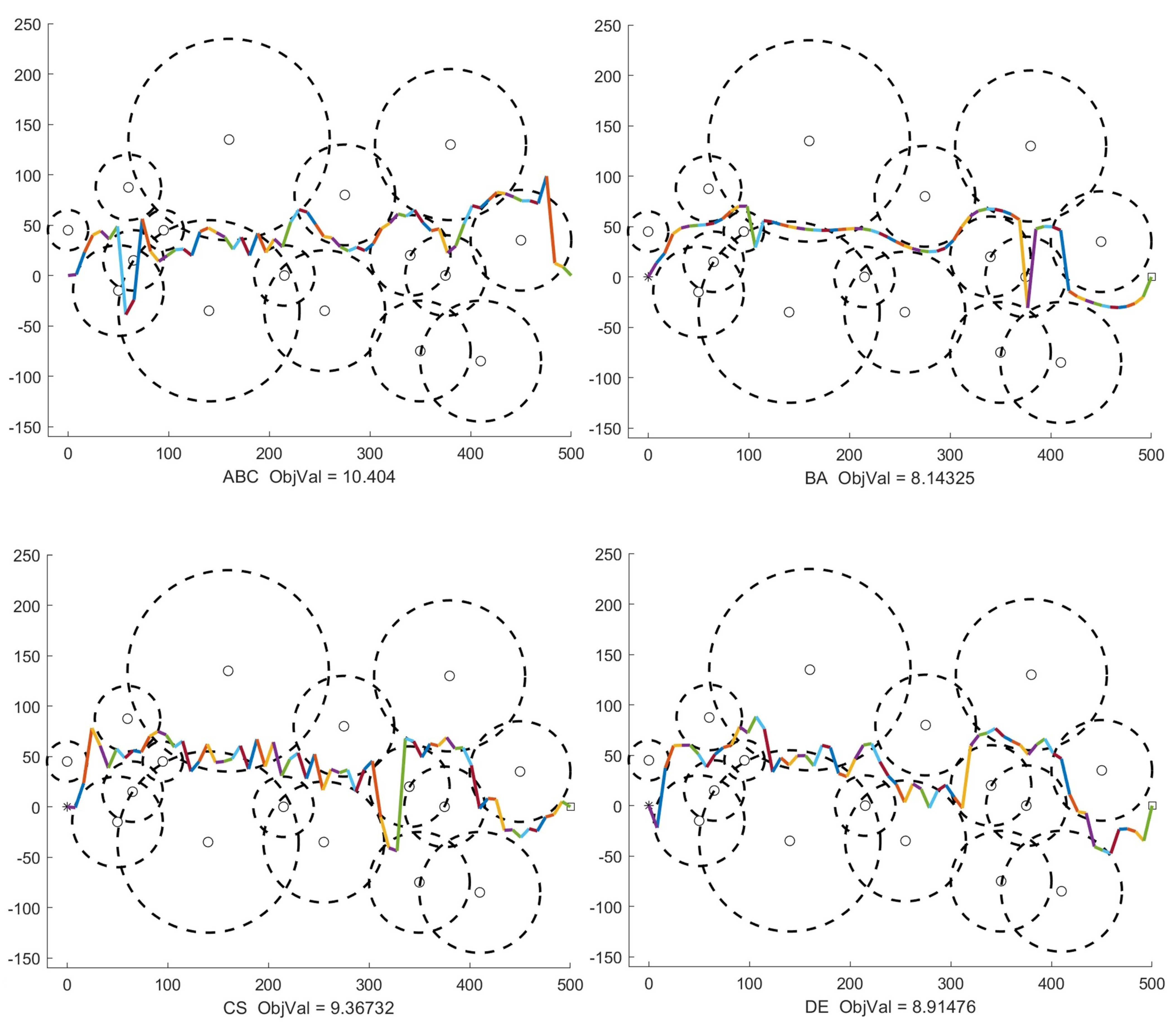
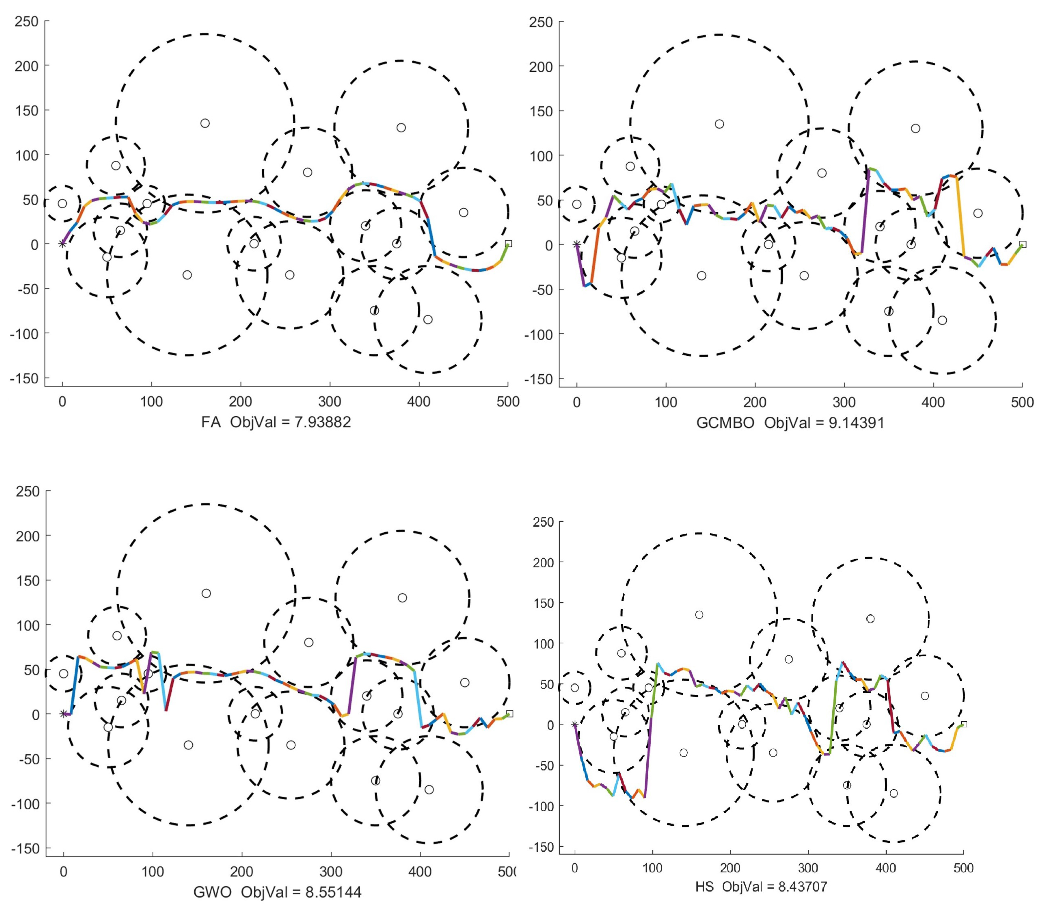
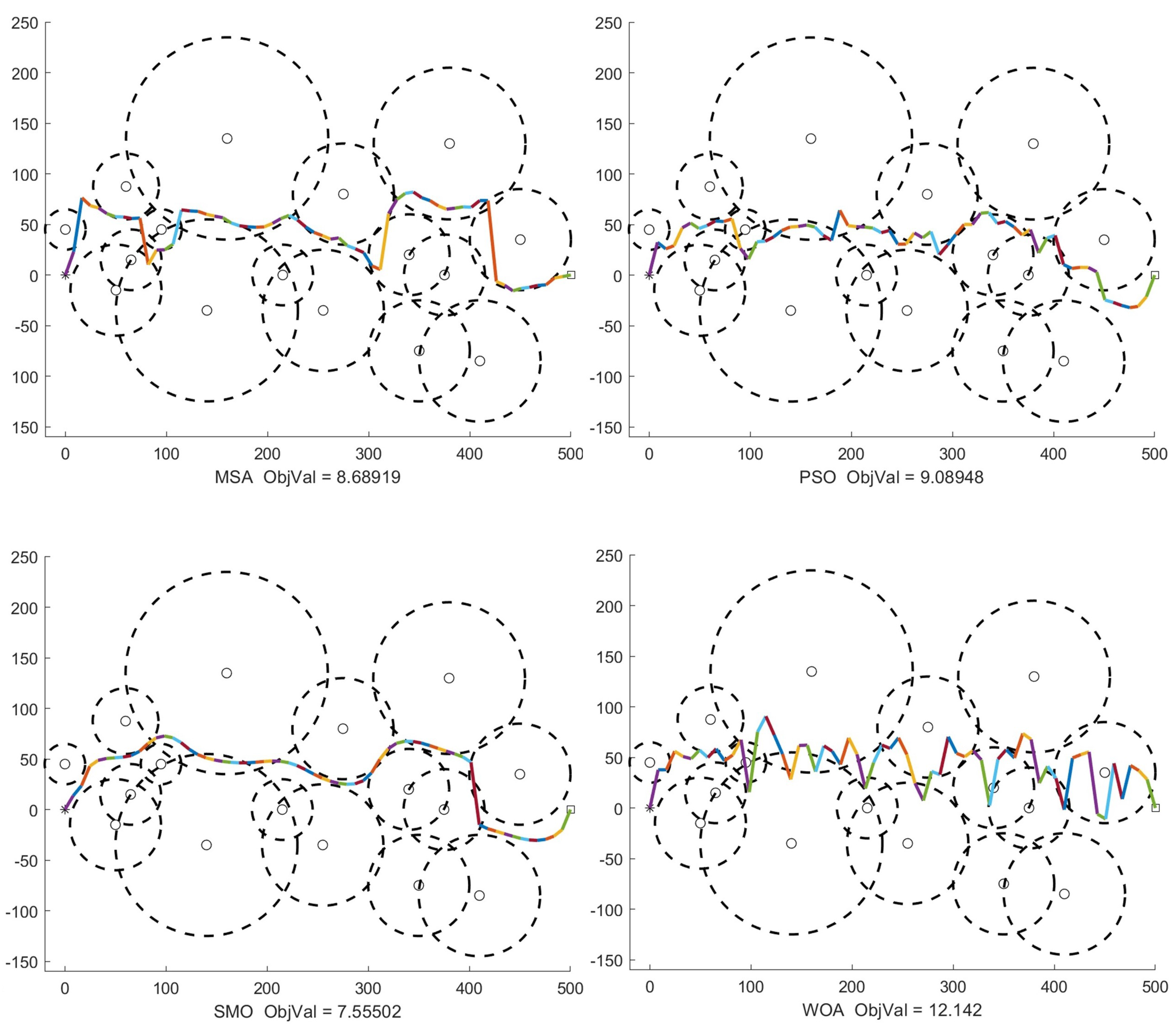
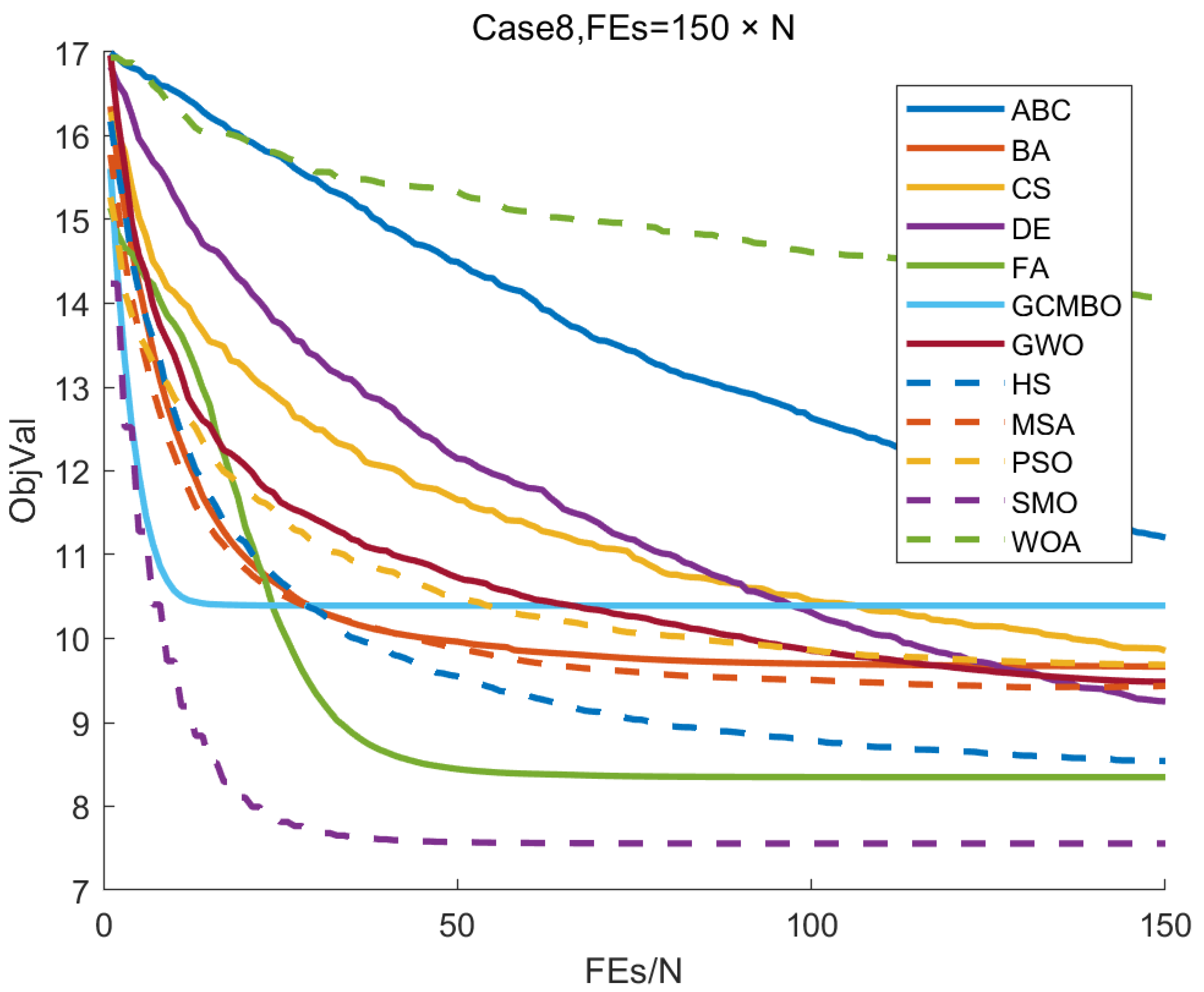
In this section, the performance of each algorithm on ten large-scale cases (D = 60) are investigated. Figure 9, Figure 10 and Figure 11 show the paths performed by different algorithms on Case 8 in large-scale. We can observe that as the dimension increases, all the algorithms perform much worse except SMO. As depicted in Figure 9, Figure 10 and Figure 11, we can notice that three algorithms including BA, FA, and SMO can provide the smooth paths. Compared with the paths in Figure 3, Figure 4 and Figure 5 and Figure 6, Figure 7 and Figure 8, it can be seen that the performance decreases significantly with the increasing dimension. Most algorithms cannot generate the successful paths since the search ability decreases with the increasing dimension. The best, worst, average objective values and the standard deviation of each algorithm on each case are tabulated in Table 4. From Table 4, we can conclude the following observations. (a) SMO provides the best path among all those twelve algorithms while the path provided by WOA has the worst performance. Moreover, the path provided by SMO has scarcely changed when compared with the cases in small-scale and medium-scale. (b) Although FA can present the acceptable paths, FA made different steps from SMO. That’s the reason why the objective value of FA is larger than that of SMO. (c) Based on the std deviation, it reveals that SMO can provide the most stable paths over multiple independent runs among all the algorithms. Moreover, the convergence rate of Case 8 under the large-scale problems is presented in Figure 12. We can observe that most algorithms can obtain the best results within less than 150 fitness evaluations. SMO can perform the best paths. However, ABC, DE and WOA cannot reach the convergence point due to the scant number of fitness evaluations of the large scale. It can be concluded that SMO has superiority over other compared algorithms with good robustness.
4.6. Stability of the Number of Fitness Evaluations
Generally, the number of iterations is often used for the criteria of termination. However, the number of fitness evaluations depends on the unique feature of each algorithm. The different procedure of each algorithm causes the different number of fitness evaluations in an iteration. Therefore, it is common to use the number of fitness evaluations as the termination threshold instead of the number of iterations [22]. Selecting a proper number of fitness evaluations is a challenging task. If the number of fitness evaluations is not enough, the optimal results can not be obtained. Otherwise, it would be wasted if the number of fitness evaluations is too big because the best result has been found very early.
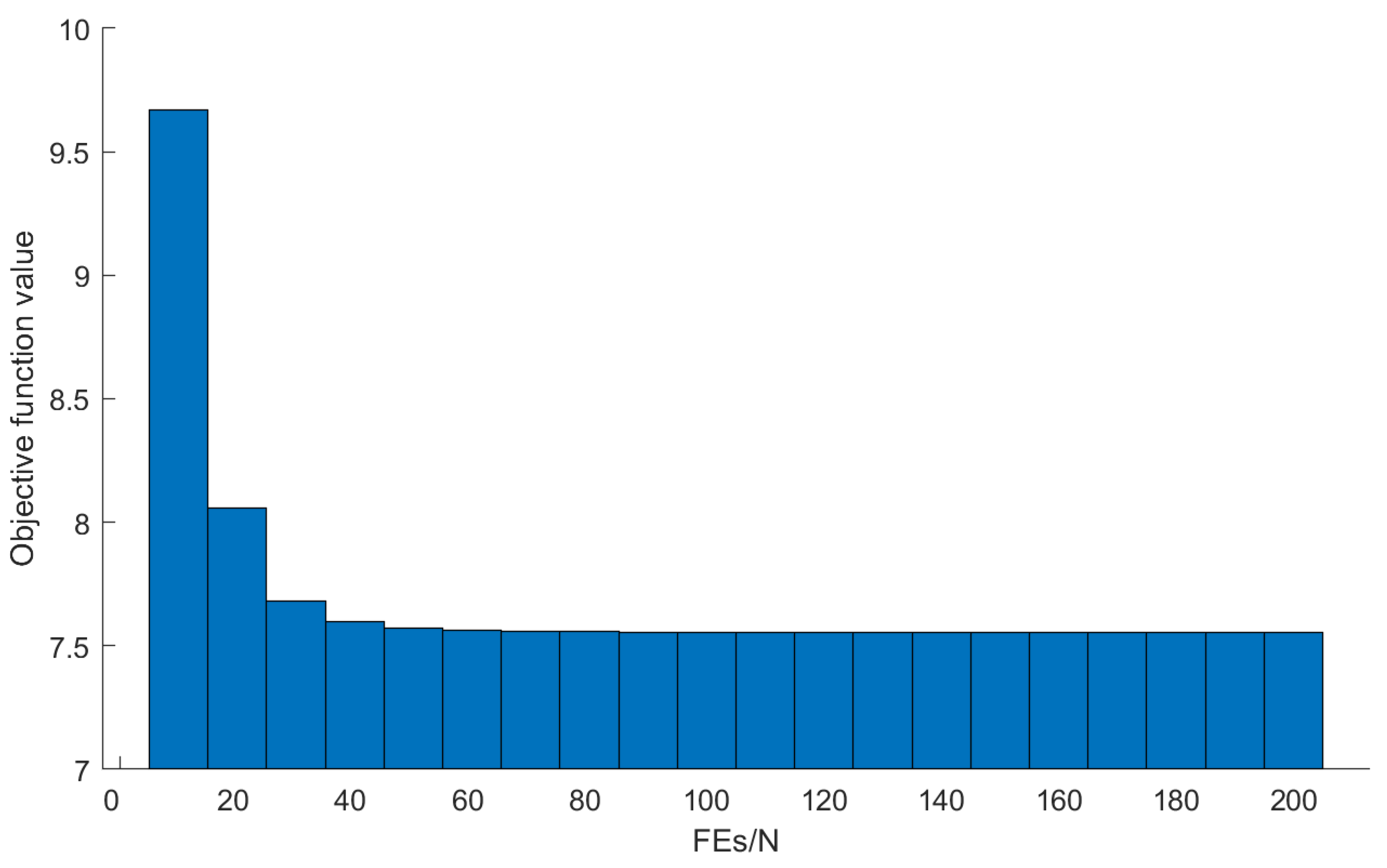
Table 2, Table 3 and Table 4 show that SMO obtains the best paths among all the algorithms for UCAV path-planning problem. To discuss the stability of for SMO, a convergence analysis based on the number of fitness evaluations is conducted on Case 8 under the large-scale problems. As depicted in Figure 13, we can observe that the best result has been obtained at times, which is far less than . This indicates that SMO has great optimizing capabilities for the UCAV path-planning problems.
5. Conclusions
This study provides a comparison of twelve SI algorithms for the UCAV path-planning problem. We survey twelve algorithms from relevant studies and apply them to UCAV path-planning. In the experiment, thirty UCAV path-planning cases are employed to verify the performance of each algorithm. The experimental results demonstrate that SMO is superior to other algorithms from different perspectives. The main contributions of this study are as follows:
- Twelve SI algorithms including ABC, BA, CS, DE, FA, GCMBO, GWO, HS, MSA, PSO, SMO, and WOA, are applied to UCAV path-planning problem by reviewing a number of papers.
- Thirty cases in different scales including ten small-scale cases with D = 20, ten medium-scale cases with D = 30, and ten large-scale cases with D = 60 are designed to demonstrate the effectiveness of each algorithm.
- A comprehensive analysis of each algorithm to address the UCAV path-planning problem is conducted from the perspective of path quality, stability, and convergence. The experimental results demonstrate that SMO exhibits better performance in discovering the safe path than the other SI algorithms.
For the UCAV path-planning problems in different scales, SMO performs the best in average while WOA delivers an obvious inferiority in obtaining good average results. In particular, SMO can provide the best average results over 25 independent runs on Case 2 in small-scale, medium-scale, and large-scale. The std deviation of SMO on each case is equal or very close to zero, which demonstrates the strong robustness of SMO. However, SMO still might get trapped into local optimum in some cases. There are two main reasons for this phenomenon: only the terminal point of each step is considered in the path-planning model, resulting in a phenomenon that a path that goes through the center of the threat has a lower objective value than that detours the threat. Another reason is that it is not necessary to generate a high-dimensional solution depending on the reality.
In the future, SMO-based algorithms should be developed based on the analysis of SMO by exploring other special strategies to enhance the efficiency. They can be applied to other route planning problems. Moreover, we will focus on designing effective methods to construct UCAV path-planning models in three-dimension.
Author Contributions
Methodology, H.Z.; supervision, X.L.; validation, Y.W.; visualization, Y.W.; writing—original draft, H.Z.; writing—review & editing, Z.M. All authors have read and agreed to the published version of the manuscript.
Funding
This research is supported by the National Natural Science Foundation of China under Grant No. 62076109, and funded by the Natural Science Foundation of Jilin Province under Grant No. 20190103006JH. Health and Medical Research Fund, the Food and Health Bureau, the Government of the Hong Kong Special Administrative Region [07181426], and the funding from Hong Kong Institute for Data Science (HKIDS) at City University of Hong Kong. The work described in this paper was partially supported by two grants from City University of Hong Kong (CityU 11202219, CityU 11203520), National Natural Science Foundation of China under Grant No. 32000464.
Institutional Review Board Statement
Not applicable.
Informed Consent Statement
Not applicable.
Conflicts of Interest
The authors declare no conflict of interest.
References
- Kabamba, P.T.; Meerkov, S.M.; Zeitz, F.H., III. Optimal path planning for unmanned combat aerial vehicles to defeat radar tracking. J. Guid. Control Dyn. 2006, 29, 279–288. [Google Scholar] [CrossRef]
- Sud, A.; Andersen, E.; Curtis, S.; Lin, M.; Manocha, D. Real-time path planning for virtual agents in dynamic environments. In Proceedings of the 2007 IEEE Virtual Reality Conference, Charlotte, NC, USA, 10–14 March 2007; pp. 91–98. [Google Scholar]
- Xin, H.; Chen, Q.; Wang, Y.; Jia, G.; Hou, Z. An Optimal Path Planning Method for UCAV in Terminal of Target Strike. In Proceedings of the 2019 Chinese Control and Decision Conference (CCDC), Nanchang, China, 3–5 June 2019; pp. 3672–3676. [Google Scholar]
- You, S.; Gao, L.; Diao, M. Real-time path planning based on the situation space of UCAVS in a dynamic environment. Microgravity Sci. Technol. 2018, 30, 899–910. [Google Scholar] [CrossRef]
- Chen, H.X.; Nan, Y.; Yang, Y. A two-stage method for UCAV TF/TA path planning based on approximate dynamic programming. Math. Probl. Eng. 2018, 2018, 1092092. [Google Scholar] [CrossRef]
- Wei, Z.; Huang, C.; Han, T.; Dong, K.; Li, Y. UCAVs online collaborative path planning method based on dynamic task allocation. In Proceedings of the 2018 Chinese Control and Decision Conference (CCDC), Shenyang, China, 9–11 June 2018; pp. 872–877. [Google Scholar]
- Pehlivanoglu, Y.V. A new vibrational genetic algorithm enhanced with a Voronoi diagram for path planning of autonomous UAV. Aerosp. Sci. Technol. 2012, 16, 47–55. [Google Scholar] [CrossRef]
- Zhang, S.; Zhou, Y.; Li, Z.; Pan, W. Grey wolf optimizer for unmanned combat aerial vehicle path planning. Adv. Eng. Softw. 2016, 99, 121–136. [Google Scholar] [CrossRef] [Green Version]
- Wang, G.G.; Chu, H.E.; Mirjalili, S. Three-dimensional path planning for UCAV using an improved bat algorithm. Aerosp. Sci. Technol. 2016, 49, 231–238. [Google Scholar] [CrossRef]
- Yi, J.H.; Lu, M.; Zhao, X.J. Quantum inspired monarch butterfly optimisation for UCAV path planning navigation problem. Int. J. Bio-Inspired Comput. 2020, 15, 75–89. [Google Scholar] [CrossRef]
- Pan, J.S.; Liu, N.; Chu, S.C. A hybrid differential evolution algorithm and its application in unmanned combat aerial vehicle path planning. IEEE Access 2020, 8, 17691–17712. [Google Scholar] [CrossRef]
- Huang, H.; Zhuo, T. Multi-model cooperative task assignment and path planning of multiple UCAV formation. Multimed. Tools Appl. 2019, 78, 415–436. [Google Scholar] [CrossRef]
- Dewangan, R.K.; Shukla, A.; Godfrey, W.W. Three dimensional path planning using Grey wolf optimizer for UAVs. Appl. Intell. 2019, 49, 2201–2217. [Google Scholar] [CrossRef]
- Paszkiel, S.; Sikora, M. The Use of Brain-Computer Interface to Control Unmanned Aerial Vehicle. In Proceedings of the Conference on Automation, Warsaw, Poland, 27–29 March 2019; pp. 583–598. [Google Scholar]
- Parpinelli, R.S.; Lopes, H.S. New inspirations in swarm intelligence: A survey. Int. J. Bio-Inspired Comput. 2011, 3, 1–16. [Google Scholar] [CrossRef]
- Yang, X.S.; Cui, Z.; Xiao, R.; Gandomi, A.H.; Karamanoglu, M. Swarm Intelligence and Bio-Inspired Computation: Theory and Applications; Elsevier: Waltham, MA, USA, 2013. [Google Scholar]
- Blum, C.; Li, X. Swarm intelligence in optimization. In Swarm Intelligence; Springer: Berlin/Heidelberg, Germany, 2008; pp. 43–85. [Google Scholar]
- Chakraborty, A.; Kar, A.K. Swarm intelligence: A review of algorithms. In Nature-Inspired Computing and Optimization; Springer: Berlin/Heidelberg, Germany, 2017; pp. 475–494. [Google Scholar]
- Wolpert, D.H.; Macready, W.G. No free lunch theorems for optimization. IEEE Trans. Evol. Comput. 1997, 1, 67–82. [Google Scholar] [CrossRef] [Green Version]
- Bansal, J.C.; Sharma, H.; Jadon, S.S.; Clerc, M. Spider monkey optimization algorithm for numerical optimization. Memetic Comput. 2014, 6, 31–47. [Google Scholar] [CrossRef]
- Ma, H.; Ye, S.; Simon, D.; Fei, M. Conceptual and numerical comparisons of swarm intelligence optimization algorithms. Soft Comput. 2017, 21, 3081–3100. [Google Scholar] [CrossRef]
- Li, X.; Wong, K.C. A comparative study for identifying the chromosome-wide spatial clusters from high-throughput chromatin conformation capture data. IEEE/ACM Trans. Comput. Biol. Bioinform. 2017, 15, 774–787. [Google Scholar] [CrossRef]
- Gunavathi, C.; Premalatha, K. A comparative analysis of swarm intelligence techniques for feature selection in cancer classification. Sci. World J. 2014, 2014, 693831. [Google Scholar] [CrossRef] [PubMed] [Green Version]
- Parpinelli, R.S.; Teodoro, F.R.; Lopes, H.S. A comparison of swarm intelligence algorithms for structural engineering optimization. Int. J. Numer. Methods Eng. 2012, 91, 666–684. [Google Scholar] [CrossRef]
- Li, B.; Gong, L.; Zhao, C. Unmanned combat aerial vehicles path planning using a novel probability density model based on Artificial Bee Colony algorithm. In Proceedings of the 2013 Fourth International Conference on Intelligent Control and Information Processing (ICICIP), Beijing, China, 9–11 June 2013; pp. 620–625. [Google Scholar] [CrossRef]
- Yang, X.S. A new metaheuristic bat-inspired algorithm. In Nature Inspired Cooperative Strategies for Optimization (NICSO 2010); Springer: Berlin/Heidelberg, Germany, 2010; pp. 65–74. [Google Scholar]
- Yang, X.S.; Deb, S. Cuckoo search via Lévy flights. In Proceedings of the 2009 World Congress on Nature & Biologically Inspired Computing (NaBIC), Coimbatore, India, 9–11 December 2009; pp. 210–214. [Google Scholar]
- Storn, R.; Price, K. Differential evolution—A simple and efficient heuristic for global optimization over continuous spaces. J. Glob. Optim. 1997, 11, 341–359. [Google Scholar] [CrossRef]
- Yang, X.S. Firefly algorithm, Levy flights and global optimization. In Research and Development in Intelligent Systems XXVI; Springer: Berlin/Heidelberg, Germany, 2010; pp. 209–218. [Google Scholar]
- Wang, G.G.; Zhao, X.; Deb, S. A novel monarch butterfly optimization with greedy strategy and self-adaptive. In Proceedings of the 2015 Second International Conference on Soft Computing and Machine Intelligence (ISCMI), Hong Kong, China, 23–24 November 2015; pp. 45–50. [Google Scholar]
- Mirjalili, S.; Mirjalili, S.M.; Lewis, A. Grey wolf optimizer. Adv. Eng. Softw. 2014, 69, 46–61. [Google Scholar] [CrossRef] [Green Version]
- Omran, M.G.; Mahdavi, M. Global-best harmony search. Appl. Math. Comput. 2008, 198, 643–656. [Google Scholar] [CrossRef]
- Wang, G.G. Moth search algorithm: A bio-inspired metaheuristic algorithm for global optimization problems. Memetic Comput. 2018, 10, 151–164. [Google Scholar] [CrossRef]
- Mirjalili, S.; Lewis, A. The whale optimization algorithm. Adv. Eng. Softw. 2016, 95, 51–67. [Google Scholar] [CrossRef]
- Geem, Z.W.; Kim, J.H.; Loganathan, G.V. A new heuristic optimization algorithm: Harmony search. Simulation 2001, 76, 60–68. [Google Scholar] [CrossRef]
Figure 1.
The schematic diagram for combat field modeling. The X and Y axles are the length and width of the horizontal battlefield. Note that all nodes are linked up to form a feasible path. During the flight, all threats are supposed to be avoid.
Figure 1.
The schematic diagram for combat field modeling. The X and Y axles are the length and width of the horizontal battlefield. Note that all nodes are linked up to form a feasible path. During the flight, all threats are supposed to be avoid.

Figure 2.
A case with ten threats. The horizontal axis is the length of the battlefield and the vertical axis is the width of the battlefield. The unit can be any unit that represents the length.
Figure 2.
A case with ten threats. The horizontal axis is the length of the battlefield and the vertical axis is the width of the battlefield. The unit can be any unit that represents the length.

Figure 3.
The comparison performance of different swarm intelligence algorithms including artificial bee colony algorithm (ABC), bat algorithm (BA), cuckoo search (CS), differential evolution (DE) for Case 8 with .
Figure 3.
The comparison performance of different swarm intelligence algorithms including artificial bee colony algorithm (ABC), bat algorithm (BA), cuckoo search (CS), differential evolution (DE) for Case 8 with .

Figure 4.
The comparison performance of different swarm intelligence algorithms including firefly algorithm (FA), monarch butterfly optimization with greedy strategy (GCMBO), grey wolf optimization (GWO), harmony search (HS) for Case 8 with .
Figure 4.
The comparison performance of different swarm intelligence algorithms including firefly algorithm (FA), monarch butterfly optimization with greedy strategy (GCMBO), grey wolf optimization (GWO), harmony search (HS) for Case 8 with .

Figure 5.
The comparison performance of different swarm intelligence algorithms including moth search algorithm (MSA), particle swarm optimization (PSO), spider monkey optimization (SMO), and whale optimization algorithm (WOA) for Case 8 with .
Figure 5.
The comparison performance of different swarm intelligence algorithms including moth search algorithm (MSA), particle swarm optimization (PSO), spider monkey optimization (SMO), and whale optimization algorithm (WOA) for Case 8 with .

Figure 6.
The comparison performance of different swarm intelligence algorithms including ABC, BA, CS and DE for Case 8 with .
Figure 6.
The comparison performance of different swarm intelligence algorithms including ABC, BA, CS and DE for Case 8 with .

Figure 7.
The comparison performance of different swarm intelligence algorithms including FA, GCMBO, GWO and HS for Case 8 with .
Figure 7.
The comparison performance of different swarm intelligence algorithms including FA, GCMBO, GWO and HS for Case 8 with .

Figure 8.
The comparison performance of different swarm intelligence algorithms including MSA, PSO, SMO and WOA for Case 8 with .
Figure 8.
The comparison performance of different swarm intelligence algorithms including MSA, PSO, SMO and WOA for Case 8 with .

Figure 9.
The comparison performance of different swarm intelligence algorithms including ABC, BA, CS and DE for Case 8 with .
Figure 9.
The comparison performance of different swarm intelligence algorithms including ABC, BA, CS and DE for Case 8 with .

Figure 10.
The comparison performance of different swarm intelligence algorithms FA, GCMBO, GWO and HS for Case 8 with .
Figure 10.
The comparison performance of different swarm intelligence algorithms FA, GCMBO, GWO and HS for Case 8 with .

Figure 11.
The comparison performance of different swarm intelligence algorithms MSA, PSO, SMO and WOA for Case 8 with .
Figure 11.
The comparison performance of different swarm intelligence algorithms MSA, PSO, SMO and WOA for Case 8 with .

Figure 12.
The convergence rate of different SI algorithm for Case 8 with large-scale. The horizontal axis denotes the number of fitness evaluations divided by the size of the population N, which is the iteration times. The vertical axle is the average objective value over 25 runs.
Figure 12.
The convergence rate of different SI algorithm for Case 8 with large-scale. The horizontal axis denotes the number of fitness evaluations divided by the size of the population N, which is the iteration times. The vertical axle is the average objective value over 25 runs.

Figure 13.
Convergence behavior of SMO. The horizontal axis denotes the number of fitness evaluations divided by N, which is the iteration times, and the vertical axis denotes the average objective value.
Figure 13.
Convergence behavior of SMO. The horizontal axis denotes the number of fitness evaluations divided by N, which is the iteration times, and the vertical axis denotes the average objective value.


Table 1.
An algorithmic parameter summary of twelve swarm intelligence (SI) algorithms.
| Algorithm | Biological Motivation | Parameter | Exploration Mechanism |
|---|---|---|---|
| ABC [25] | Honey Collecting Behavior of Bee Colony | trial = 0.1·FEs | An employed bee denotes a feasible solution, the unemployed bees do local search. |
| BA [26] | Echolocation of bats | Fmin = 1 Fmax = 4 A = 2.5 r0 = 1 alpha = 0.97 gamma = 2.5 | Bats fly randomly with a velocity at a position with a fixed frequency, varying wavelength and loudness to search for prey. |
| CS [27] | brood parasitism | beta = 1.5 | Eggs with better quality have more chances to survive. |
| DE [28] | Mutation and crossover of chromosome | F = 0.5 CR = 0.1 | All the individuals conduct the mutation and crossover operators |
| FA [29] | The blinking behavior of fireflies | alpha = 0.5 beta = 1 gamma = 0.01 theta = | A firefly can be attracted by others that are brighter than it. |
| GCMBO [30] | The migration behavior of monarch butterflies | p = 0.5 peri = 0.5 beta = 1.5 Smax = 1 BAR = 0.8 | The monarch butterflies in Land 1 and Land 2 are composed of the whole population, and the worse subgroup moves to the better one randomly. |
| GWO [31] | Encircling and hunting behavior of gray wolves | None | Take average of the three leader wolves. |
| HS [32] | Search for better harmony | HMCR = 0.9 PAR = 0.2 BAR = L·0.01 | A random dimension of the solution vector is picked for updating. |
| MSA [33] | Phototropism of moths | Smax = 1 beta = 0.5 phy = | A moth can be attracted by lights. When it’s far away, it will fly straight, or it will do random fly. |
| PSO [25] | Bird migration | c1 = 1.4962 c2 = 1.4962 w = 0.7298 | Individuals update their positions by their velocity and current positions. |
| SMO [20] | Fission-fusion system of spider monkey | MG = N/4 GLL = N LLL = D·N pr = 0.375 | Divide the group into a certain number of subgroups if stagnated. |
| WOA [34] | Encircling and preying behavior of whales | a = 5 -iter·/FEs b = 1.5 A = 2·a·rand-a C = 2·rand I = rand·2-1 p = rand | Do exploration by spiral updating. |
Table 2.
Performance comparison of different swarm intelligence algorithms for small-scale uninhabited combat air vehicle (UCAV) path-planning. The best, worst, average and standard deviation over 25 runs of each algorithm for ten cases are provided. The best values are in bold.
Table 2.
Performance comparison of different swarm intelligence algorithms for small-scale uninhabited combat air vehicle (UCAV) path-planning. The best, worst, average and standard deviation over 25 runs of each algorithm for ten cases are provided. The best values are in bold.
| Case 1 | Case 2 | Case 3 | Case 4 | Case 5 | Case 6 | Case 7 | Case 8 | Case 9 | Case 10 | ||
|---|---|---|---|---|---|---|---|---|---|---|---|
| ABC | 4.02419 4.22836 4.14491 0.05401 | 1.55182 1.71690 1.61041 0.03998 | 1.69836 1.87450 1.75736 0.04304 | 2.00564 2.34539 2.15096 0.08755 | 2.10935 2.37855 2.25920 0.06807 | 2.08304 2.39144 2.22037 0.07445 | 3.17832 3.53045 3.32170 0.09690 | 3.40311 3.69164 3.57828 0.07010 | 3.03541 3.45004 3.22825 0.10477 | 2.78953 3.15891 2.96556 0.09753 | Best Worst Average Std deviation |
| BA | 4.06832 4.55974 4.26404 0.13025 | 1.47449 1.81447 1.64581 0.09027 | 1.69652 2.28030 1.96575 0.15832 | 2.08734 2.82178 2.36674 0.22850 | 2.10935 2.37855 2.25920 0.06807 | 2.22917 2.85678 2.51155 0.14218 | 3.08888 3.97422 3.60318 0.25250 | 3.46535 4.36706 3.91960 0.25231 | 2.98014 4.85309 3.84687 0.36851 | 2.92027 3.67888 3.36492 0.19427 | Best Worst Average Std deviation |
| CS | 4.03220 4.18388 4.09087 0.04843 | 1.49796 1.59921 1.54096 0.02967 | 1.64508 1.69286 1.66259 0.01233 | 1.96107 2.09279 1.99728 0.02792 | 2.10634 2.27114 2.16817 0.03341 | 1.99048 2.29661 2.10217 0.06515 | 3.11039 3.17957 3.15049 0.01860 | 3.40549 3.52887 3.44878 0.03094 | 2.95024 3.13843 3.02180 0.04584 | 2.79610 2.98839 2.85613 0.03932 | Best Worst Average Std deviation |
| DE | 4.02880 4.12530 4.07083 0.02170 | 1.50325 1.61329 1.53355 0.02514 | 1.63592 1.65845 1.64587 0.00658 | 1.94842 1.98861 1.96551 0.01144 | 2.08429 2.17788 2.12827 0.02312 | 2.11028 2.27987 2.19684 0.05239 | 3.09575 3.11684 3.10590 0.00563 | 3.38597 3.44025 3.40691 0.01165 | 2.93400 3.03077 2.97620 0.02309 | 2.78577 2.85924 2.81632 0.02036 | Best Worst Average Std deviation |
| FA | 3.98033 4.41767 4.18981 0.12989 | 1.47449 1.68793 1.57556 0.05752 | 1.61806 1.87802 1.66160 0.09639 | 1.95343 2.38280 2.10564 0.11432 | 2.08232 2.16536 2.08971 0.01857 | 1.97192 2.37051 2.15159 0.11398 | 3.11165 3.91961 3.62811 0.17178 | 3.47924 3.94338 3.60082 0.09872 | 2.91277 3.48155 3.31600 0.16063 | 2.77118 2.90343 2.85962 0.05177 | Best Worst Average Std deviation |
| GCMBO | 4.09861 4.61633 4.35093 0.13047 | 1.67749 1.96159 1.81784 0.07070 | 1.85437 2.40352 2.06054 0.14633 | 2.18445 2.85107 2.50667 0.16969 | 2.36318 3.94095 2.82242 0.32262 | 2.30052 2.84723 2.61433 0.13625 | 3.41527 4.20496 3.69809 0.23585 | 3.66108 4.46385 4.03578 0.16473 | 3.41110 4.13645 3.78223 0.25659 | 3.14582 3.76983 3.44099 0.18228 | Best Worst Average Std deviation |
| GWO | 3.99392 4.30288 4.11663 0.08042 | 1.51986 1.68710 1.59373 0.04810 | 1.61942 2.04082 1.69373 0.11241 | 1.93603 2.44024 2.06802 0.11212 | 2.03664 2.29864 2.10303 0.07381 | 1.94153 2.33305 2.07372 0.10230 | 3.13821 3.86821 3.43738 0.18621 | 3.43052 4.04737 3.64063 0.17303 | 2.92174 3.79556 3.18509 0.29254 | 2.76177 3.19019 2.90663 0.12241 | Best Worst Average Std deviation |
| HS | 3.96302 4.08843 4.02537 0.04445 | 1.47787 1.64180 1.51918 0.05018 | 1.62287 1.66543 1.63472 0.00879 | 1.91028 1.95335 1.93401 0.01022 | 2.04462 2.13986 2.08287 0.02929 | 1.94352 2.09013 2.00332 0.05375 | 3.09337 3.11112 3.09912 0.00433 | 3.37481 3.49135 3.38584 0.02250 | 2.91970 2.97966 2.94064 0.01508 | 2.76248 2.95445 2.84744 0.05337 | Best Worst Average Std deviation |
| MSA | 4.04798 4.50929 4.22686 0.10797 | 1.53099 1.84316 1.67300 0.08239 | 1.62493 1.95150 1.75042 0.12822 | 1.97107 2.69312 2.24537 0.18634 | 2.05623 2.71180 2.18386 0.16910 | 1.99782 2.40953 2.21390 0.12837 | 3.17287 4.12896 3.59242 0.28264 | 3.41803 4.54438 3.68847 0.25160 | 2.97542 3.83439 3.40229 0.23950 | 2.85214 3.39389 3.09557 0.16223 | Best Worst Average Std deviation |
| PSO | 4.20501 4.46044 4.34820 0.07488 | 1.51803 1.73712 1.61448 0.05803 | 1.65574 1.88085 1.71962 0.05977 | 2.04092 2.37730 2.24712 0.10038 | 2.11362 2.48445 2.20476 0.08953 | 2.07533 2.37978 2.25161 0.08583 | 3.27830 3.93095 3.56903 0.14681 | 3.41937 3.74395 3.58126 0.08585 | 3.04995 3.47818 3.19644 0.11082 | 2.91570 3.34519 3.05964 0.10172 | Best Worst Average Std deviation |
| WOA | 4.62953 5.20931 4.89909 0.15727 | 1.73079 2.31805 2.05008 0.14920 | 2.13197 2.62385 2.35926 0.15173 | 2.74961 3.41324 3.04231 0.17118 | 2.57314 3.68988 3.16261 0.34023 | 2.50992 3.31362 2.89391 0.18900 | 3.89892 4.74324 4.32977 0.23192 | 4.27351 5.32713 4.75819 0.27605 | 3.85183 5.07037 4.45843 0.32343 | 3.48746 4.47647 4.00377 0.26026 | Best Worst Average Std deviation |
| SMO | 3.95556 3.98066 3.95903 0.00708 | 1.47449 1.50205 1.47564 0.00550 | 1.61806 1.61807 1.61806 0.00000 | 1.91451 1.91451 1.91451 0.00000 | 2.03334 2.03753 2.03366 0.00084 | 1.93365 1.97235 1.94550 0.01591 | 3.08887 3.08887 3.08887 0.00000 | 3.36897 3.36897 3.36897 0.00000 | 2.82486 2.90891 2.86160 0.03739 | 2.71818 2.77118 2.74048 0.01317 | Best Worst Average Std deviation |
Table 3.
Performance comparison of different swarm intelligence algorithms for medium-scale UCAV path-planning. The best, worst, average and standard deviation over 25 runs of each algorithm for ten cases are provided. The best values are in bold.
Table 3.
Performance comparison of different swarm intelligence algorithms for medium-scale UCAV path-planning. The best, worst, average and standard deviation over 25 runs of each algorithm for ten cases are provided. The best values are in bold.
| Case 1 | Case 2 | Case 3 | Case 4 | Case 5 | Case 6 | Case 7 | Case 8 | Case 9 | Case 10 | ||
|---|---|---|---|---|---|---|---|---|---|---|---|
| ABC | 5.65076 6.08632 5.91296 0.11717 | 1.81274 2.21838 2.06146 0.09269 | 2.21308 2.66935 2.43436 0.11428 | 2.61850 3.34486 3.04549 0.15528 | 3.07183 3.81704 3.42027 0.19154 | 2.99558 3.50178 3.20440 0.15197 | 4.69979 5.23968 4.96524 0.14500 | 5.00439 5.64008 5.37282 0.16854 | 4.15122 5.21948 4.74236 0.30034 | 3.92333 4.66747 4.39441 0.18788 | Best Worst Average Std deviation |
| BA | 5.48759 6.34582 5.88167 0.21399 | 1.77326 2.15701 1.92546 0.09885 | 1.90156 2.66515 2.32488 0.22482 | 2.46398 3.86547 3.01165 0.36855 | 3.04086 4.76201 3.64501 0.40921 | 2.98142 3.93330 3.27451 0.22400 | 4.29104 5.56908 5.07498 0.34054 | 4.80065 6.15390 5.46074 0.34729 | 4.46421 5.82402 5.16717 0.35195 | 4.01242 5.00900 4.43730 0.27593 | Best Worst Average Std deviation |
| CS | 5.65665 5.92436 5.77357 0.08256 | 1.84557 2.08908 1.96735 0.05361 | 2.06679 2.20753 2.14125 0.04085 | 2.52672 2.74825 2.62565 0.06282 | 2.83356 3.07316 2.96140 0.07160 | 2.76835 3.16608 2.95712 0.10896 | 4.26268 4.53927 4.41239 0.08635 | 4.66472 4.98162 4.80506 0.08756 | 4.09219 4.42214 4.23083 0.08683 | 3.78004 4.13001 3.99211 0.10191 | Best Worst Average Std deviation |
| DE | 5.59849 5.80682 5.72977 0.05331 | 1.85658 1.99903 1.92201 0.03472 | 1.98665 2.11889 2.05332 0.02914 | 2.47533 2.65453 2.53862 0.05005 | 2.75406 2.95975 2.85785 0.05363 | 2.92717 3.25458 3.06828 0.08813 | 4.14844 4.31031 4.22782 0.04530 | 4.58752 4.76395 4.68243 0.05005 | 3.98125 4.22699 4.08003 0.05506 | 3.69402 3.92693 3.81012 0.06165 | Best Worst Average Std deviation |
| FA | 5.33925 5.96082 5.69696 0.16364 | 1.69999 1.97332 1.81607 0.06355 | 1.88776 2.37488 2.09590 0.19622 | 2.40394 3.09543 2.67013 0.23080 | 2.55200 2.68846 2.56051 0.02813 | 2.48963 3.02501 2.73860 0.16406 | 4.68407 5.22605 4.98621 0.11673 | 4.57875 5.16279 4.78427 0.15727 | 3.84686 4.65075 4.42518 0.18589 | 3.51198 4.40823 3.76076 0.18211 | Best Worst Average Std deviation |
| GCMBO | 5.78657 6.30673 6.06380 0.13623 | 2.01830 2.48651 2.21077 0.12100 | 2.39372 3.22922 2.66618 0.18939 | 2.90994 3.62314 3.19552 0.19989 | 3.14760 4.24778 3.67160 0.28268 | 3.12060 4.16561 3.49270 0.23986 | 4.54533 5.70627 5.02587 0.26947 | 5.18538 6.44745 5.63362 0.30288 | 4.54210 5.75663 5.02665 0.35624 | 4.21660 5.02060 4.63974 0.22564 | Best Worst Average Std deviation |
| GWO | 5.34573 5.73215 5.56816 0.09551 | 1.73384 2.09779 1.89774 0.08944 | 1.91593 2.31262 2.05335 0.14233 | 2.31796 3.11416 2.59894 0.23897 | 2.52626 2.94557 2.70787 0.11710 | 2.34983 3.13474 2.69087 0.21214 | 4.36972 5.11318 4.69397 0.21956 | 4.55366 5.39305 4.92003 0.22447 | 3.78445 5.13422 4.18506 0.34129 | 3.52735 4.56521 3.92667 0.25907 | Best Worst Average Std deviation |
| HS | 5.35354 5.54654 5.45640 0.06811 | 1.72596 1.95107 1.80369 0.06155 | 1.94628 2.03262 1.98097 0.02289 | 2.30948 2.42990 2.35934 0.02769 | 2.56904 2.73681 2.67809 0.04163 | 2.38619 2.56015 2.48170 0.03772 | 4.09788 4.20235 4.12535 0.02180 | 4.49091 4.63989 4.53653 0.04085 | 3.78557 3.96182 3.86109 0.04647 | 3.57972 3.93696 3.74365 0.10070 | Best Worst Average Std deviation |
| MSA | 5.60787 6.19402 5.83312 0.14906 | 1.83507 2.12393 1.97181 0.08224 | 1.93295 2.55960 2.16728 0.19211 | 2.36184 3.59325 2.74959 0.30554 | 2.47755 3.04907 2.68769 0.11633 | 2.45798 3.55619 2.87685 0.27158 | 4.22888 5.45793 4.86628 0.31305 | 4.54239 5.54283 5.01900 0.27074 | 3.78452 5.21095 4.38520 0.43944 | 3.86997 4.43788 4.17755 0.15929 | Best Worst Average Std deviation |
| PSO | 5.98899 6.47456 6.22912 0.14031 | 1.88923 2.23412 2.00588 0.07914 | 2.07140 2.49609 2.24133 0.12277 | 2.84528 3.81686 3.19410 0.22559 | 2.70623 3.13978 2.87739 0.11863 | 2.75534 3.33932 3.08111 0.14866 | 4.63766 5.53994 5.07385 0.23081 | 4.64379 5.27142 4.93601 0.16315 | 4.04411 4.95748 4.40160 0.20275 | 3.92172 4.57736 4.22134 0.15953 | Best Worst Average Std deviation |
| WOA | 6.61783 7.61292 7.17790 0.26680 | 2.39543 3.10127 2.74974 0.21759 | 2.77779 3.69120 3.23990 0.26836 | 4.11051 4.91711 4.42680 0.23448 | 3.97166 5.72925 4.67329 0.41286 | 3.43633 4.62582 4.20823 0.26723 | 5.56872 7.04486 6.41485 0.32993 | 5.94858 7.96494 6.93741 0.52289 | 5.55131 7.38154 6.33971 0.42879 | 5.47799 6.84366 5.97577 0.35668 | Best Worst Average Std deviation |
| SMO | 5.29633 5.31442 5.29896 0.00504 | 1.67871 1.70088 1.68123 0.00606 | 1.88776 1.88782 1.88779 0.00001 | 2.24303 2.24332 2.24308 0.00006 | 2.45917 2.55200 2.46334 0.01848 | 2.29663 2.39585 2.32247 0.03772 | 4.04452 4.04452 4.04452 0.00000 | 4.42171 4.42171 4.42171 0.00000 | 3.60465 3.69517 3.66045 0.03406 | 3.46036 3.47025 3.46117 0.00207 | Best Worst Average Std deviation |
Table 4.
Performance comparison of different swarm intelligence algorithms for large-scale UCAV path-planning. The best, worst, average and standard deviation over 25 runs of each algorithm for ten cases are provided. The best values are in bold.
Table 4.
Performance comparison of different swarm intelligence algorithms for large-scale UCAV path-planning. The best, worst, average and standard deviation over 25 runs of each algorithm for ten cases are provided. The best values are in bold.
| Case 1 | Case 2 | Case 3 | Case 4 | Case 5 | Case 6 | Case 7 | Case 8 | Case 9 | Case 10 | ||
|---|---|---|---|---|---|---|---|---|---|---|---|
| ABC | 11.28948 12.45483 11.82839 0.26937 | 3.52370 4.23379 3.88755 0.19687 | 4.62416 5.74213 5.20526 0.28801 | 5.27874 7.18993 6.61427 0.40836 | 6.57170 8.43326 7.70273 0.53493 | 6.29494 7.31052 6.85397 0.30889 | 9.21089 11.21872 10.35821 0.51347 | 10.40403 11.79650 11.20326 0.37926 | 8.69186 11.61452 10.48508 0.64202 | 8.05864 10.06662 9.33420 0.43498 | Best Worst Average Std deviation |
| BA | 10.07523 11.34526 10.84208 0.30431 | 2.36412 3.25754 2.86006 0.21337 | 3.03078 4.03706 3.49477 0.28616 | 3.56815 5.66683 4.62838 0.56681 | 4.98585 7.15262 5.88189 0.49289 | 4.56774 6.17443 5.38978 0.40968 | 7.93291 9.93842 9.25137 0.47881 | 8.14325 10.89560 9.66495 0.63872 | 7.42097 10.30115 8.97254 0.71529 | 6.66584 9.39240 7.80731 0.62308 | Best Worst Average Std deviation |
| CS | 11.02470 11.97790 11.56665 0.23127 | 3.27712 3.75498 3.48136 0.11770 | 4.05966 4.62767 4.32548 0.15375 | 5.11979 5.84504 5.50343 0.19957 | 6.08151 6.84316 6.41659 0.20786 | 5.68708 6.76414 6.35895 0.25384 | 8.80291 9.59481 9.22561 0.21309 | 9.36732 10.38349 9.85457 0.26566 | 8.60296 9.52930 9.02512 0.25167 | 7.74665 8.67339 8.33623 0.24913 | Best Worst Average Std deviation |
| DE | 10.81923 11.41790 11.17581 0.12184 | 3.05663 3.39874 3.26770 0.07760 | 3.65372 4.03394 3.84818 0.09269 | 4.48336 5.17994 4.83894 0.13693 | 5.54172 6.05136 5.80331 0.12447 | 6.41216 6.83525 6.62057 0.13182 | 8.09821 8.57801 8.35366 0.12208 | 8.91476 9.62494 9.24848 0.19508 | 7.88400 8.58606 8.23071 0.15882 | 7.28692 8.06260 7.66489 0.18647 | Best Worst Average Std deviation |
| FA | 9.74002 10.93901 10.27844 0.28866 | 2.35975 3.00926 2.55646 0.16495 | 2.68280 3.65493 3.31374 0.25383 | 4.03736 5.25249 4.56729 0.28831 | 3.92864 4.06381 3.94498 0.03587 | 3.73500 4.81286 4.39317 0.27751 | 8.34560 9.54978 8.81935 0.24707 | 7.93882 8.82559 8.34753 0.26402 | 7.17874 8.26742 7.64827 0.25245 | 6.13161 6.50968 6.20375 0.08006 | Best Worst Average Std deviation |
| GCMBO | 10.75231 11.98840 11.22760 0.26693 | 3.06132 3.82188 3.47342 0.19764 | 3.86643 5.00522 4.55553 0.29868 | 5.03095 6.57505 5.67516 0.42072 | 6.12203 7.82037 6.86026 0.43076 | 5.80826 6.81993 6.34602 0.28311 | 8.74677 10.11920 9.21887 0.33034 | 9.14391 11.09870 10.39141 0.46456 | 8.46155 10.22534 9.27781 0.55259 | 7.92789 9.64340 8.66641 0.40073 | Best Worst Average Std deviation |
| GWO | 9.78014 10.95061 10.29231 0.26782 | 2.47045 2.98815 2.77026 0.13709 | 2.89594 4.12009 3.45772 0.33983 | 3.53668 5.12438 4.15567 0.40610 | 3.97649 5.22502 4.45868 0.27546 | 3.78132 5.29693 4.44264 0.35927 | 8.09615 9.59289 8.78866 0.35898 | 8.55144 10.66260 9.48210 0.55005 | 7.10976 8.88337 8.00236 0.55676 | 6.40047 7.86799 7.11720 0.36556 | Best Worst Average Std deviation |
| HS | 9.82004 10.34328 10.13713 0.13847 | 2.64062 2.94563 2.79976 0.08645 | 3.32102 3.69148 3.47388 0.08576 | 4.00540 4.17452 4.08885 0.05438 | 4.88691 5.32263 5.09346 0.12405 | 4.03190 4.61613 4.36115 0.12310 | 7.48906 7.83730 7.65542 0.10100 | 8.37265 8.71449 8.54144 0.07568 | 6.83698 7.54559 7.17944 0.16236 | 6.75239 7.42808 7.06739 0.15036 | Best Worst Average Std deviation |
| MSA | 10.32344 11.86800 10.94214 0.38142 | 2.87248 3.90167 3.18777 0.25169 | 2.96156 4.12512 3.66284 0.29124 | 4.22400 5.86799 4.91878 0.53616 | 4.16115 5.36838 4.67980 0.33062 | 4.57433 5.89082 5.17434 0.33019 | 8.64102 10.12286 9.40588 0.40917 | 8.68919 10.38032 9.43296 0.45564 | 6.70786 9.10212 7.89441 0.62966 | 7.00489 8.67775 7.82829 0.52474 | Best Worst Average Std deviation |
| PSO | 11.50878 12.60180 12.04514 0.31066 | 3.03016 3.99445 3.51718 0.23999 | 3.37450 4.32213 3.87036 0.26719 | 5.62018 6.85294 6.14793 0.30718 | 4.83580 6.22815 5.39061 0.30680 | 5.43883 6.66681 5.97327 0.29597 | 9.65874 11.35977 10.45275 0.45541 | 9.08948 10.23278 9.68565 0.31336 | 7.99124 9.50469 8.88687 0.39625 | 7.12936 8.94442 8.07835 0.41303 | Best Worst Average Std deviation |
| WOA | 13.07540 14.99135 14.15923 0.45608 | 4.35528 5.95417 5.32378 0.34832 | 5.29230 7.10852 6.13517 0.44914 | 7.27906 9.70345 8.50375 0.59170 | 8.05213 10.45468 9.09167 0.71228 | 6.75522 9.73888 8.24215 0.75644 | 11.90830 14.05014 12.90899 0.62665 | 12.14199 15.23174 14.05722 0.73750 | 11.27253 14.75277 12.75595 0.76187 | 11.16476 13.14390 11.96014 0.46090 | Best Worst Average Std deviation |
| SMO | 9.18336 9.23077 9.19360 0.01229 | 2.23828 2.25006 2.24292 0.00351 | 2.68036 2.68237 2.68106 0.00051 | 3.16685 3.16958 3.16777 0.00070 | 3.70875 3.93383 3.72058 0.04451 | 3.36677 3.64994 3.43767 0.10010 | 6.88067 6.88070 6.88068 0.00001 | 7.55502 7.55514 7.55506 0.00003 | 5.98846 5.99026 5.98890 0.00037 | 5.54869 5.59005 5.55364 0.00895 | Best Worst Average Std deviation |
Publisher’s Note: MDPI stays neutral with regard to jurisdictional claims in published maps and institutional affiliations. |
© 2021 by the authors. Licensee MDPI, Basel, Switzerland. This article is an open access article distributed under the terms and conditions of the Creative Commons Attribution (CC BY) license (http://creativecommons.org/licenses/by/4.0/).
Share and Cite
MDPI and ACS Style
Zhu, H.; Wang, Y.; Ma, Z.; Li, X. A Comparative Study of Swarm Intelligence Algorithms for UCAV Path-Planning Problems. Mathematics 2021, 9, 171. https://0-doi-org.brum.beds.ac.uk/10.3390/math9020171
AMA Style
Zhu H, Wang Y, Ma Z, Li X. A Comparative Study of Swarm Intelligence Algorithms for UCAV Path-Planning Problems. Mathematics. 2021; 9(2):171. https://0-doi-org.brum.beds.ac.uk/10.3390/math9020171
Chicago/Turabian StyleZhu, Haoran, Yunhe Wang, Zhiqiang Ma, and Xiangtao Li. 2021. "A Comparative Study of Swarm Intelligence Algorithms for UCAV Path-Planning Problems" Mathematics 9, no. 2: 171. https://0-doi-org.brum.beds.ac.uk/10.3390/math9020171
Note that from the first issue of 2016, this journal uses article numbers instead of page numbers. See further details here.