Spatio-Temporal Patterns of CO₂ Emissions and Influencing Factors in China Using ESDA and PLS-SEM

Abstract

Controlling carbon dioxide (CO₂) emissions is the foundation of China’s goals to reach its carbon peak by 2030 and carbon neutrality by 2060. This study aimed to explore the spatial and temporal patterns and driving factors of CO₂ emissions in China. First, we constructed a conceptual model of the factors influencing CO₂ emissions, including economic growth, industrial structure, energy consumption, urban development, foreign trade, and government management. Second, we selected 30 provinces in China from 2006 to 2019 as research objects and adopted exploratory spatial data analysis (ESDA) methods to analyse the spatio-temporal patterns and agglomeration characteristics of CO₂ emissions. Third, on the basis of 420 data samples from China, we used partial least squares structural equation modelling (PLS-SEM) to verify the validity of the conceptual model, analyse the reliability and validity of the measurement model, calculate the path coefficient, test the hypothesis, and estimate the predictive power of the structural model. Fourth, multigroup analysis (MGA) was used to compare differences in the influencing factors for CO₂ emissions during different periods and in various regions of China. The results and conclusions are as follows: (1) CO₂ emissions in China increased year by year from 2006 to 2019 but gradually decreased in the eastern, central, and western regions. The eastern coastal provinces show spatial agglomeration and CO₂ emission hotspots. (2) Confirmatory analysis showed that the measurement model had high reliability and validity; four latent variables (industrial structure, energy consumption, economic growth, and government management) passed the hypothesis test in the structural model and are the determinants of CO₂ emissions in China. Meanwhile, economic growth is a mediating variable of industrial structure, energy consumption, foreign trade, and government administration on CO₂ emissions. (3) The calculated results of the R² and Q² values were 76.3% and 75.4%, respectively, indicating that the structural equation model had substantial explanatory and high predictive power. (4) Taking two development stages and three main regions as control groups, we found significant differences between the paths affecting CO₂ emissions, which is consistent with China’s actual development and regional economic pattern. This study provides policy suggestions for CO₂ emission reduction and sustainable development in China.

1. Introduction

Climate change is a major global challenge faced by humanity today and has attracted extensive attention from the international community [1]. Countries have committed to reducing greenhouse gases to address climate change caused by greenhouse gases such as carbon dioxide (CO₂) [2,3]. In 2016, 178 parties signed the Paris Agreement, which became the third landmark international legal text to tackle climate change, following the UN Framework Convention on Climate Change in 1992 and the Kyoto Protocol in 1997, shaping global climate governance patterns. The Paris Agreement obliges all parties to commit to a long-term greenhouse gas emission reduction strategy for the mid-21st century until 2020 to promote early and significant reductions in global emissions. At the 75th UN General Assembly in September 2020, China proposed reaching its carbon peak by 2030 and striving to achieve carbon neutrality by 2060. A carbon peak is reached when carbon emissions (mainly CO₂) no longer increase. Carbon neutrality refers to a state of net-zero emissions after efforts to reduce or offset CO₂ emissions. China’s carbon peak and carbon neutrality targets are consistent with the Paris Agreement and key to achieving the 1.5 °C global temperature decrease target.

China is at a critical stage of industrialisation and urbanisation. CO₂ emissions are continuing to increase, and many energy conservation and emission-reduction activities could be implemented. China has made continuous attempts to construct low-carbon cities, establish a circular economy, conserve resources, encourage an environment-friendly society, and pursue other paths to green development, with some positive results [4,5]. During the 14th Five-Year Plan (2021–2025), China will enter a critical period in which the country will focus on CO₂ reduction, promote the synergy and efficiency of pollution and CO₂ reduction, facilitate a comprehensive green transformation in economic and social development, realise a qualitative change in the improvement of ecological and environmental quality, and promote major changes in the way society functions. China will pursue its long-term goals of peak carbon and carbon neutrality; promote economic and social transformation; and accelerate the building of a green, low-carbon economic system. It will also continue to play a positive and constructive leading role in the international community, promote the establishment of a new cooperation mechanism for global climate governance, and strive to build a community with a common future for humanity [6,7,8].

In 2020, China’s CO₂ emissions totalled 9894 billion tons, the highest in the world, and thus China came under great pressure to reduce emissions. China has a vast land area, and there are great differences between regions in the natural environment, development stage, population distribution, industrial structure, urbanisation, and other characteristics. The main factors that affect CO₂ emissions and their degree of influence are also different [9,10]. Therefore, it is of great theoretical and practical significance to explore the spatio-temporal patterns and driving factors of CO₂ emissions in different regions within China to formulate energy conservation and emission reduction policies to achieve the goals of peak carbon and carbon neutrality.

The determinants of CO₂ emissions are diverse, and the relationships between these driving forces are complex. Therefore, it is of great significance for China’s ability to further control CO₂ emissions in the future to identify the influencing factors of CO₂ emissions and further clarify the causal relationships between these driving forces. First, we identified the driving factors affecting CO₂ emissions and constructed a conceptual model. We then analysed the spatio-temporal evolution of CO₂ emissions in China by using exploratory spatial data analysis (ESDA). We analysed the effect paths of the driving factors affecting CO₂ emissions using partial least squares structural equation modelling (PLS-SEM) methods. Finally, we propose policy suggestions for China’s sustainable development.

2. Literature Review and Hypotheses

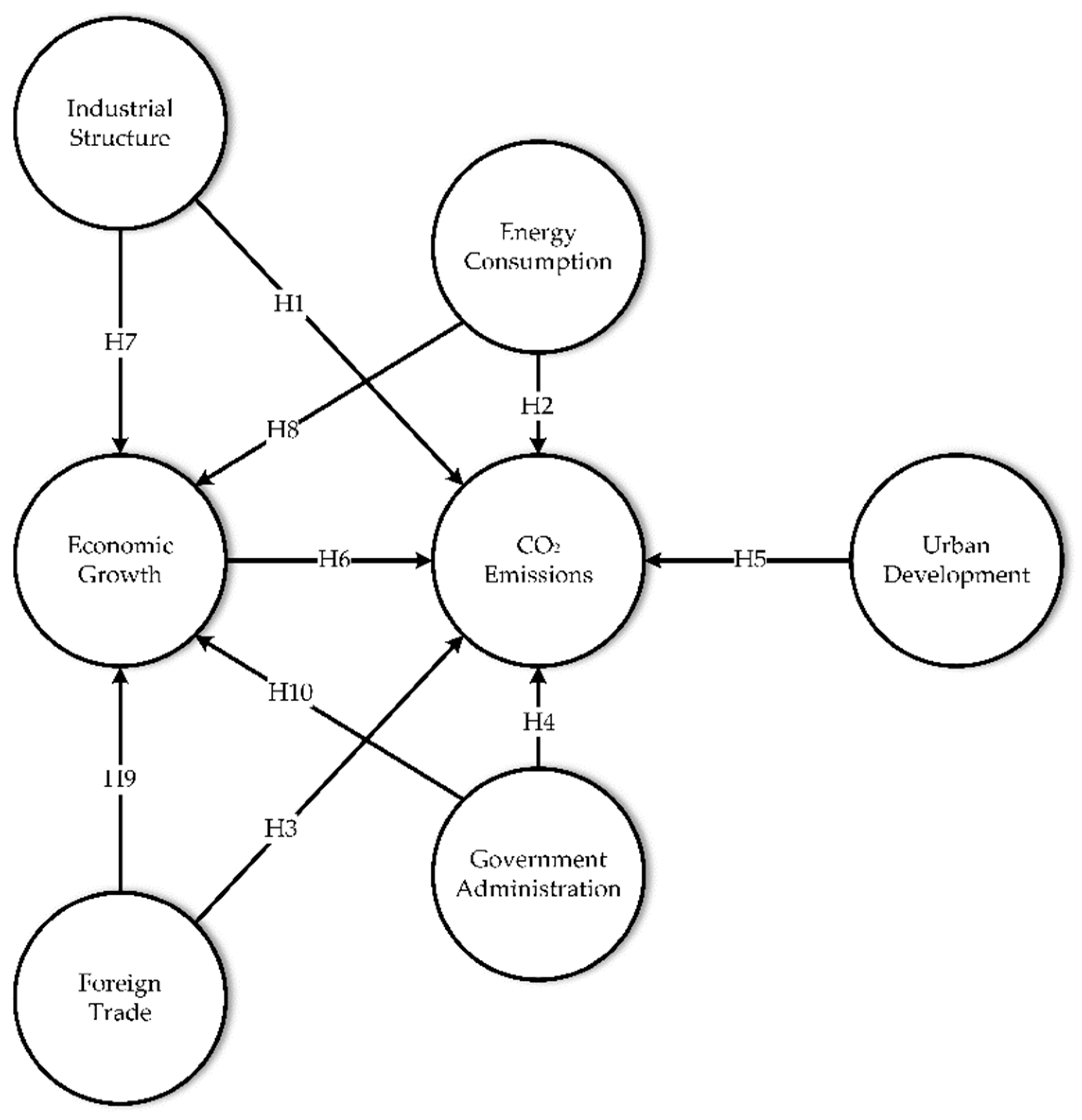
Increased CO₂ emissions result from economic growth, industrial structure, energy consumption, and other factors. Clarifying the key factors that affect CO₂ emission for research is of critical importance. However, most studies have focused on the relationship between specific factors and CO₂ emissions, while few studies have systematically explored the factors and their degree of influence on CO₂ emissions. Therefore, this study attempts to construct a theoretical framework concerning CO₂ emissions and explores the direction and intensity of each driving factor. We discuss the factors influencing CO₂ emissions in six dimensions: economic growth, industrial structure, energy consumption, urban development, foreign trade, and government management. We then hypothesise that these factors influence CO₂ emissions and construct a conceptual model (Figure 1).

2.1. Industrial Structure

With adjustments and developments of industrial structures, the CO₂ emissions of an economic system also change. The theory of industrial structural evolution holds that, during the process of economic development, the labour force shifts from primary industries dominated by agriculture to secondary industries dominated by factory production of goods, which is the main industry for CO₂ emissions. The higher the proportional contribution of the secondary industry to the total output value, the greater the threat to the environment and the higher CO₂ emissions. In particular, the higher the proportion of energy-intensive industries, the greater the CO₂ emissions. As the economy continues to expand, the labour force moves to tertiary industries dominated by services. In this process, the total CO₂ emissions will continue to increase, but the growth rate will decelerate. Additionally, different industrial structures have different impacts on CO₂ emissions. Some scholars have studied the influencing factors on CO₂ emissions in different industrial sectors, such as transportation, agriculture, industry, and tourism, and results vary from study to study [11,12]. Zheng et al. explored interregional differences in industry, construction, and transportation; warehousing industries had a significantly positive impact on interregional differences in CO₂ emissions from 2007 to 2016 [13]. Li et al. suggested that governments should increase the proportion of high-tech industries through technological progress, vigorously develop resource-saving and environment-friendly tertiary industries, and develop a low-carbon economy by promoting clean production technology [14]. Many scholars have found that industrial structure upgrading has a significant positive impact on economic growth, thereby promoting CO₂ emission reduction [15,16]. On the basis of the aforementioned literature, we propose the following hypothesis:

Hypothesis 1 (H1):

Industrial structure contributes to more CO₂ emissions.

2.2. Energy Consumption

Economic growth heavily depends on energy consumption, which is a direct source of CO₂ emissions. Energy consumption quantity, intensity, and structure have some impact on CO₂ emissions. Economic development is inseparable from the use of all kinds of energy. The larger the economy grows, the more energy is consumed, and the more CO₂ emissions rise. Wang et al. concluded that reducing energy intensity could, to a large extent, reduce CO₂ emission intensity. By optimising industrial structure, CO₂ emission intensity could also be inhibited [10]. Energy intensity is the energy consumed per unit of output and is used to measure energy efficiency. The higher the level of technological progress, the less energy is wasted [17]. The structure of energy consumption has an important impact on CO₂ emissions. The carbon content of energy used in economic construction determines CO₂ emissions; the higher the carbon content, the greater the CO₂ emissions, and vice versa [18]. Xu et al. analysed the dynamic relationships between CO₂ emissions, economic growth, and the consumption of various fossil fuels in China and found that increasing coal and petroleum consumption significantly promoted CO₂ emissions. However, natural gas offers a cleaner substitute for other fossil fuels [19]. Thus, the impact of energy consumption on CO₂ emissions is clear. China is in a period of highly industrialised development, and coal-fired power generation is still the main form of power generation. Coal-fired power plants burn much fossil fuel and emit a large amount of CO₂, although the Chinese government has regulated the power industry as a key sector [20]. However, compared with European and American countries, China still has a long way to go in terms of energy conservation and emission reduction. Therefore, the sustainable development of electric energy is the main path of a low-carbon economy. In this way, the following hypothesis is proposed:

Hypothesis 2 (H2):

Energy consumption contributes to more CO₂ emissions.

2.3. Foreign Trade

Engaging in international trade may be a factor in changing CO₂ emissions. Foreign trade is one of the principal ways to transfer CO₂ emissions through an international division of labour [21]. The expansion of foreign trade, as well as the structure and volume of foreign trade, may be factors in a country’s CO₂ emissions. It is undeniable that China’s foreign trade products are characterised by high energy consumption and low added value. The effect of import and export on CO₂ emissions is intuitively positive. However, relevant studies have found that the impact of foreign trade on CO₂ emissions may be positive [22], negative [23], or irrelevant [24], depending on both the foreign trade structure and trade volume [25] and also to the research period and region. Nevertheless, industrial transfer is one way of transferring CO₂ emissions. According to the foreign direct investment (FDI) theory, to maximise profits and reduce environmental costs, investors implement cross-border pollution transfer to transfer high-emission industries to lower-income regions, thus realising CO₂ emissions transfer. China is in a period of rapid economic development and must introduce a large amount of foreign capital for economic construction, which has a significant impact on CO₂ emissions. As the energy price is low, and the regulation of polluting industries is lower than that of higher-income countries, many export industries with high energy consumption and carbon emissions rapidly develop and become production sites for capital investment countries to transfer pollution [26]. Additionally, FDI has a technological spillover effect on CO₂ emissions that can improve the technical level of the region and reduce CO₂ emissions. Therefore, FDI affects the CO₂ emissions of the host country. On the basis of the aforementioned literature, we propose the following hypothesis:

Hypothesis 3 (H3):

Foreign trade contributes to more CO₂ emissions.

2.4. Government Administration

Government intervention may be a key factor influencing CO₂ emissions. Related studies have found that governments affect CO₂ emissions in many ways. First, governments formulate corresponding energy transition and environmental policies to constrain the CO₂ emissions of enterprises and society [17,27]. Second, governments can increase financial expenditure on environmental governance [28] and scientific and technological investment, as well as collect pollution control fees and taxes from enterprises [29] to reduce levels of environmental pollution. Third, local governments may take the initiative to relax environmental regulations to achieve regional economic growth and thereby attract investment, which results in the deterioration of regional environmental quality and an increase in CO₂ emissions. Local government decision-making competition has three effects on CO₂ emissions: market distortion, investment bias, and a race to the bottom of environmental policies.

Hypothesis 4 (H4):

Government administration contributes to reduced CO₂ emissions.

2.5. Urban Development

Urban development is an important factor affecting CO₂ emissions. First, a country’s level of urbanisation is closely related to its economic development. The larger the scale of urban development, the more CO₂ emissions increase. However, improvements in urbanisation levels can decrease CO₂ emissions and thus realise low-carbon development [30]. In the early stages of urban development, Sun found that the expansion of the scope of urbanisation promotes improvement in CO₂ emission efficiency. After the urbanisation level reaches a critical point, the economic growth rate falls behind the growth rate in CO₂ emissions [31]. Second, a large number of energy resources is necessary for infrastructure construction during the process of urbanisation, which leads to an increase in CO₂ emissions. Zhou et al. found that spatial urbanisation was positively associated with CO₂ emissions due to the new infrastructure construction and conversion of existing land [32]. Third, during urbanisation, many people migrate from rural to urban areas, and this substantial increase in the urban population also increases CO₂ emissions [33]. Improvements in economic development and urbanisation can help achieve low-carbon development in an urban agglomeration [34].

Hypothesis 5 (H5):

Urban development contributes to more CO₂ emissions.

2.6. Economic Growth

Economic growth is an important index for measuring the economic development of a country or region. According to the environmental Kuznets curve (EKC), when a country has a low level of economic development and uses few energy resources, its CO₂ emissions are low. However, with the acceleration of industrialisation, more fossil energy is needed, the degree of environmental deterioration worsens, and CO₂ emissions rise. When economic development reaches a certain level, the degree of environmental pollution and CO₂ emissions gradually decrease. Dinda et al. analysed the EKC hypothesis and postulated an inverted-U-shaped relationship between different pollutants and per capita income; that is, environmental pressure increases up to a certain level as income increases and decreases thereafter [35]. Fang et al. verified the panel EKC between economic growth and CO₂ emissions in China from 1995 to 2016 and found that, as the economy developed and GDP per capita increased, more energy was consumed, and the amount of environmental pollution increased [36]. Mardani et al. further found that CO₂ emissions were stimulated at higher or lower levels as economic growth increased or decreased. Conversely, a potential reduction in emissions harms economic growth [37].

China faces the dual pressures of economic growth and environmental protection [36]. On the one hand, China needs to reduce CO₂ emissions to jointly cope with the global climate crisis with the international community. On the other hand, China should also pay attention to domestic economic growth and social progress to enhance its national strength and improve its resilience to external environmental changes. Economic growth is a task and goal that cannot be ignored. Therefore, economic growth plays a connecting role between industrial structure, energy consumption, trade growth, government management, and carbon emissions. In recent years, China has witnessed rapid economic growth, increasing energy consumption, and a rapid increase in CO₂ emissions. In the future, China will need enough space for CO₂ emissions to reach the level of higher-income countries. Thus, as the economy continues to grow, CO₂ emissions will continue to accumulate.

Therefore, we propose the following hypotheses:

Hypothesis 6 (H6):

Economic growth contributes to more CO₂ emissions.

Hypothesis 7 (H7):

Economic growth mediates the relationship between industrial structure and CO₂ emissions.

Hypothesis 8 (H8):

Economic growth mediates the relationship between energy consumption and CO₂ emissions.

Hypothesis 9 (H9):

Economic growth mediates the relationship between foreign trade and CO₂ emissions.

Hypothesis 10 (H10):

Economic growth mediates the relationship between government administration and CO₂ emissions.

3. Materials and Methods

3.1. Study Area

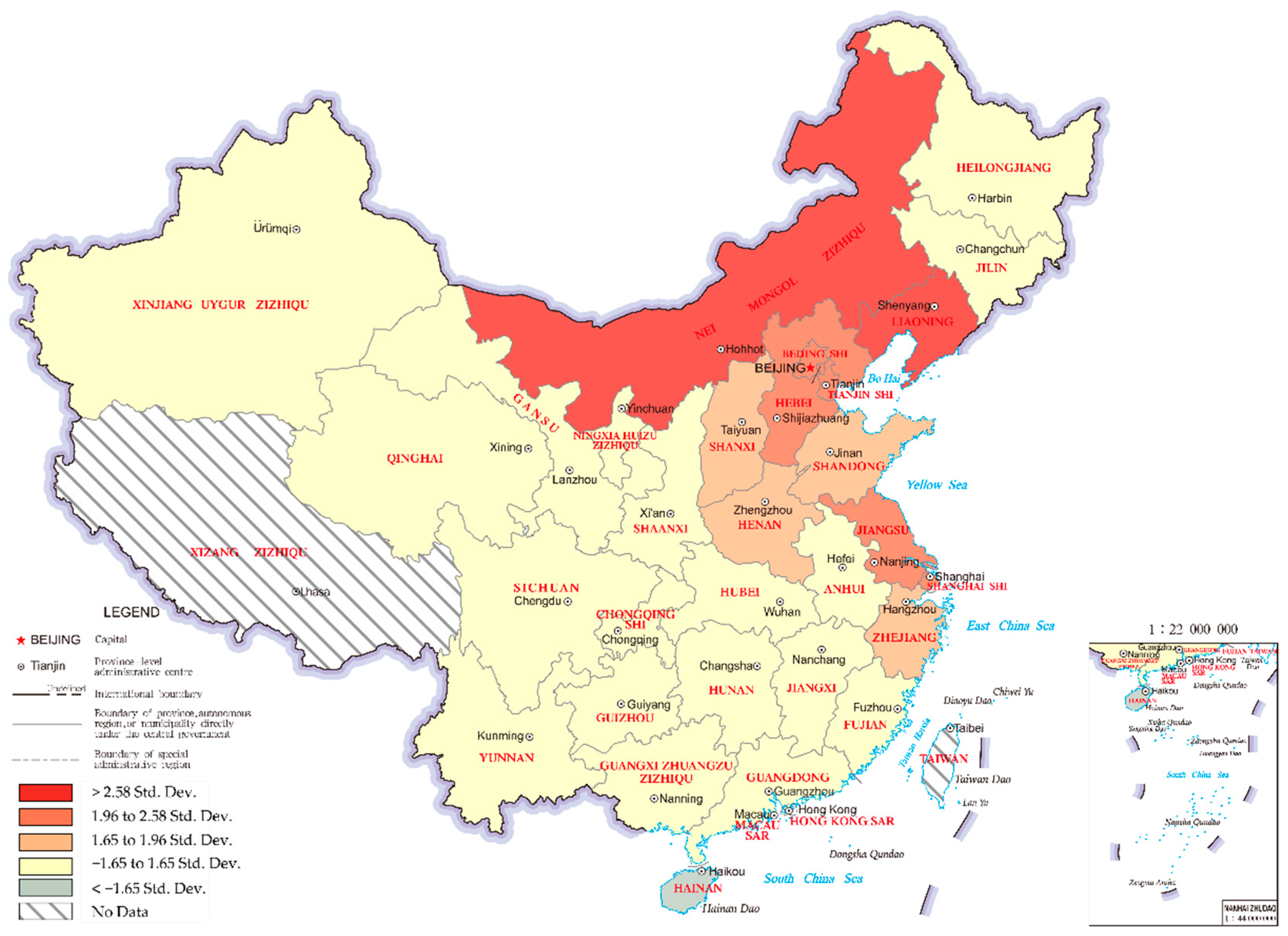
This study selected 30 provinces, autonomous regions, and municipalities as the research areas to acquire relevant statistical data, excluding Hong Kong, Macao, Taiwan, and Tibet. These areas can be divided into three main regions: eastern, central, and western.

• Eastern region: Beijing, Tianjin, Hebei, Liaoning, Shanghai, Jiangsu, Zhejiang, Fujian, Shandong, Guangdong, Guangxi, and Hainan.
• Central region: Shanxi, Henan, Anhui, Jilin, Heilongjiang, Jiangxi, Hubei, Hunan, and Inner Mongolia.
• Western region: Chongqing, Sichuan, Guizhou, Yunnan, Shaanxi, Gansu, Ningxia, Qinghai, and Xinjiang.

The CO₂ emissions of 30 provinces in China showed an overall upward trend from 2006 to 2019, increasing from 8.32 billion in 2006 to 13.92 billion in 2019, with an annual growth rate of 4.03%.

3.2. Data Collection

This study selected 420 data observations from 30 provinces, autonomous regions, and municipalities from 2006 to 2019 as research samples. The main data in this paper include CO₂ emissions and influencing factors. The former were calculated from fossil energy consumption data published in the China Statistical Yearbook of Energy (2006–2019), while the latter were mainly derived from the China Statistical Yearbook (2006–2019). Missing values were supplemented using linear interpolation with IBM SPSS Statistics 25.0 software (IBM Inc., Armonk, NY, USA).

(1)

Data on CO₂ emissions. The estimates of CO₂ emissions of provinces in China are taken from the IPCC Guidelines for the National Greenhouse Gas Emission Inventory. According to China Energy Statistical Yearbook, primary energy consumption can be divided into eight categories: coal, coke, crude oil, fuel oil, gasoline, kerosene, diesel, and natural gas. As there are so many energy sources, the total CO₂ emissions from combustion should be the sum of the CO₂ emissions from each energy source.

$$C{E}_{it}={\displaystyle \sum _{i=1}^n{E}_{ijt}\times {\omega }_j}$$

(1)

where CE_it represents the CO₂ emissions generated by energy combustion in province i in year t, E_ijt represents the burned amount of energy j in province i, ω_j represents the CO₂ emissions coefficient of energy j combustion, and n represents the eight kinds of energy.

(2)

Data for influencing factors. Following the principles of systematicity, representativeness, and availability of index selection, this study used 16 specific indicators from the six dimensions of economic development level, industrial structure, energy consumption, urban development, foreign trade, and government management, using the following specific descriptions:

(i)

Economic growth. Gross domestic product (GDP) and per capita GDP represent the level of economic growth, which can measure the impact of the economy on CO₂ emissions. Household consumption level is selected to reflect the economic conditions of people’s lives, which is an important reflection of national economic growth.

(ii)

Industrial structure. The proportion of the value added by the secondary industry to GDP can represent the industrial structure of the main source of CO₂. The proportion of industrial added value in the GDP reflects that China is still in the development stage of industrialisation at present; its main industries have high energy consumption, and that consumption will not be significantly reduced in a short time.

(iii)

Energy consumption. With China’s economic development and social progress, the production and consumption of electric energy are increasing. The power industry has become a major contributor to fossil fuel consumption and CO₂ emissions. Annual carbon emissions from electricity generation are close to 50% of the country’s total energy CO₂ emissions. Therefore, it is reasonable to take electric energy production and consumption as two indicators to measure CO₂ emissions.

(iv)

Urban development. The urban employed population reflects the agglomeration of the urban population. Urban fixed-asset investment reflects the input of urban factors. Traffic is an important source of urban CO₂ emissions, and the number of civilian vehicles can be used as an indicator to measure the impact of traffic on CO₂ emissions.

(v)

Foreign trade. The total FDI and number of FDI enterprises can reflect the investment in foreign capital; the total export–import volume is used to reflect foreign trade. As FDI and total export–import volume are denominated in U.S. dollars, the U.S. GDP deflator is used to calculate the real value for the year 2019.

(vi)

Government management. The impact of the Chinese government’s intervention on CO₂ emissions can be considered from two perspectives: financial spending and administrative management. Scientific and technological input is selected as the financial index, reflecting the government’s ability to curb CO₂ emissions by improving scientific and technological levels. Administrative management indicators include the accepted number of domestic patent applications and the authorised number of domestic patent applications, which are used to measure the impact of government and enterprises on CO₂ emissions from the perspective of science and technology.

3.3. Methods

Quantitative studies of CO₂ emissions have been a hot topic in recent years. Previous studies widely used include the Kaya identity [38,39,40]; the IPAT model [41,42,43]; the arithmetic mean divisia index (AMDI); the logarithmic mean divisia index (LMDI) [44,45,46,47]; and the stochastic impacts by regression on population, affluence, and technology (STIRPAT) model [48,49,50,51]. This study integrated ESDA and PLS-SEM to study the spatio-temporal differences and influencing factors of CO₂ emissions in China. The spatial correlation and hotspot analysis of the ESDA method intuitively reflected the spatial distribution and spatial agglomeration of CO₂ emissions. The PLS-SEM method was used to analyse the influence paths, intensity, and significance of the factors influencing CO₂ emissions.

3.3.1. ESDA

ESDA is an analytical method for exploring the spatial relevance of geographical phenomena from the perspective of spatial analysis; it is also suitable for studying the spatial agglomeration of CO₂ emissions [52,53].

Spatial Autocorrelation

Global and local autocorrelation can reveal the spatial connections and differences between research units, which are often expressed by Moran’s I. Global autocorrelation can describe the spatial correlation pattern of a whole research area; the local autocorrelation can reflect the spatial agglomeration characteristics of each unit within the region and identify high-value agglomeration and low-value agglomeration at different spatial locations. This method is suitable for representing the spatial agglomeration characteristics of CO₂ emissions in the research area [54,55]. The calculation formula is

$$I=\frac{n}{{\displaystyle \sum _{i=1}^n{(x_i-\overline{x})}^2}}·\frac{{\displaystyle \sum _{i=1}^n{\displaystyle \sum _{j=1}^n{w}_{ij}(x_i-\overline{x})(x_j-\overline{x})}}}{{\displaystyle \sum _{i=1}^n{\displaystyle \sum _{j=1}^n{w}_{ij}}}}$$

(2)

$$I_L=\frac{n(x_i-\overline{x}){\displaystyle \sum _{j=1}^n{w}_{ij}(x_j-\overline{x})}}{{\displaystyle \sum _{i=1}^n{(x_i-\overline{x})}^2}}$$

(3)

where I represents the global Moran index, and I_L represents the local Moran index. n is the number of provinces, and x_i and x_j are the CO₂ emission values of province i and province j, respectively. w_ij is the adjacency matrix between province i and province j. At the significance level, the value of the global Moran I index ranges from −1 to 1. If the value of the index is greater than 0, there is a positive spatial correlation between the two provinces; if the value is less than 0, there is a negative spatial correlation; if it is equal to 0, there is no spatial correlation. The local spatial association mode can be divided into high–high (H-H), high–low (H-L), low–high (L-H), and low–low (L-L). The global Moran index statistics can only test the global spatial correlation but cannot determine the specific spatial agglomeration region, whereas the local Moran index and the Getis–Ord G_i* local statistics can solve this problem.

Hotspots Analysis

On the basis of the Getis–Ord G_i* value, ARCGIS software can be used to automatically draw a spatial clustering graph of high and low values with statistical significance, which reveals the hotspots and coldspots of regional CO₂ emissions [56]. The formulas are as follows:

$$G_i^{*}=\frac{{\displaystyle \sum _{i=1}^n{\omega }_{i,j}{x}_j-\overline{X}}{\displaystyle \sum _{j=1}^n{\omega }_{i,j}}}{S\sqrt{\frac{n{\displaystyle \sum _{j=1}^n{\omega }_{i,j}{}^2-{\left({\displaystyle \sum _{j=1}^n{\omega }_{i,j}}\right)}^2}}{n-1}}}$$

(4)

$$S=\sqrt{\frac{{\displaystyle \sum _{j=1}^n{x}_j{}^2}}{n}-{\overline{X}}^2}$$

(5)

$$\overline{X}=\frac{{\displaystyle \sum _{j=1}^n{x}_j}}{n}$$

(6)

where x_j is the attribute value of province j, ω_ij is the spatial weight of province i and province j, and n is the total number of provinces. G_i* is the score of the z value, which reflects the spatio-temporal agglomeration characteristics of high and low CO₂ emissions.

3.3.2. PLS-SEM

PLS-SEM is used to estimate a complex causal relationship model with latent variables; it is widely used in economics, sociology, and other fields [57]. Therefore, this study is a new attempt to explore the influence of various driving factors on CO₂ emissions using PLS-SEM. The PLS-SEM model has the following three advantages: first, multiple latent variables are introduced to better reflect the path, orientation, and intensity between latent variables and CO₂ emissions; second, the complex relationships between latent variables and their causal effects can be further clarified; third, comparative analyses between control groups better reflect the temporal difference and spatial heterogeneity. PLS-SEM must generally follow four steps: model construction, hypothesis formulation, confirmatory factor analysis, and structural model analysis [58,59,60]. We also adopted multigroup analysis to understand the differences between factors affecting CO₂ emissions in different periods and regions. As both the total sample and the control sample size exceeded 100, the PLS-SEM technology of SmartPLS 3.3.3 software was suitable for testing the causal relationships proposed in the conceptual model.

Multigroup analysis (MGA) allows for testing whether pre-defined data groups have significant differences in their group-specific parameter estimates (e.g., outer weights, outer loadings, and path coefficients) [61]. In recent years, the MGA method has also been widely applied in tourism [61,62], marketing [63,64], and other fields. This study adopted MGA to analyse the difference in the impact paths on CO₂ emissions in different periods and regions. SmartPLS 3.3.3 provides outcomes of four different approaches that are based on bootstrapping results from every group.

4. Results

4.1. Spatio-Temporal Evolution Patterns and Agglomeration Characteristics of CO₂ Emissions

4.1.1. Spatio-Temporal Patterns at Different Scales

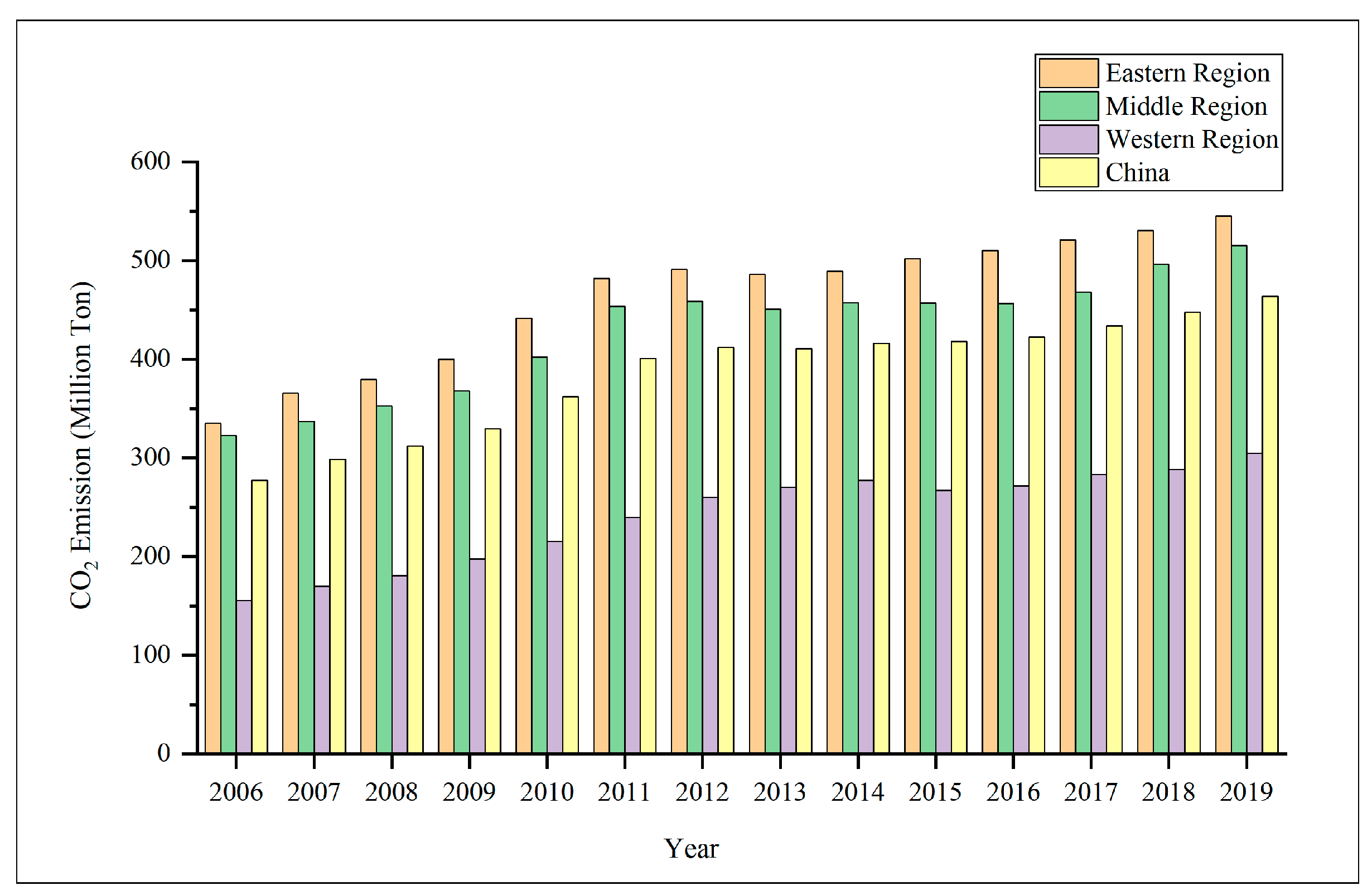
At the national scale, CO₂ emissions have been rising steadily in China, from 277.43 million tons in 2006 to 463.97 million tons in 2019, with an annual growth rate of 4.03%. From the perspective of the development stage, CO₂ emissions grew rapidly from 2006 to 2011 but slowed from 2012 to 2019, with annual growth rates of 7.63% and 1.71%, respectively (Figure 2).

At the regional scale, the average CO₂ emissions of the eastern, central, and western regions were 334.95 million tons, 322.68 million tons, and 155.49 million tons, respectively, in 2006. The average CO₂ emissions of the eastern, middle, and western regions increased to 535.34 million tons, 515.03 million tons, and 304.43 million tons in 2019, with annual growth rates of 3.82, 3.66, and 5.30%, respectively. The order of mean CO₂ emission is eastern region > central region > western region (Figure 2).

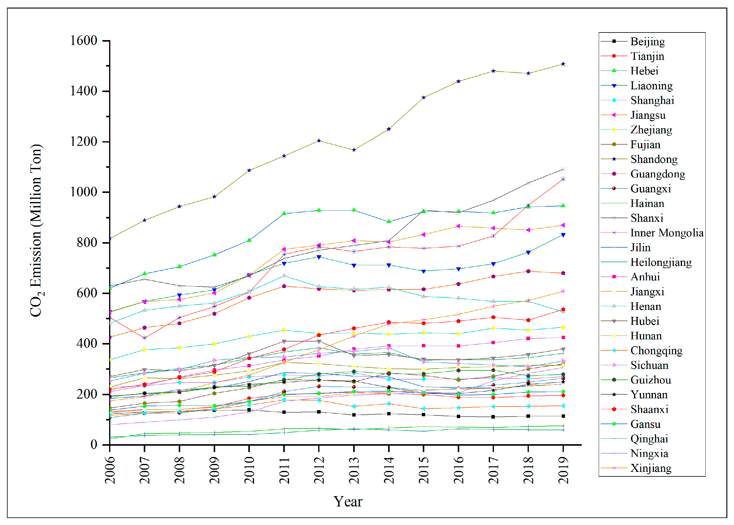
At the provincial scale, CO₂ emissions in nine provinces were higher than the national average of CO₂ emissions (277.43 million tons) in 2006, and CO₂ emissions in 11 provinces were more than the national average of CO₂ emissions (463.97 million tons) in 2019. Shandong province has always ranked first in CO₂ emissions in China, whereas Qinghai province always ranked last from 2006 to 2019. The growth rate of CO₂ emission in Beijing decreased year by year, showing a negative growth rate. The growth rate of CO₂ emissions in Shanghai and Henan remained at relatively low levels, 0.69 and 1.31%, respectively, while the growth rates for Ningxia and Xinjiang, although they were located in the western region, were 10.82 and 10.05%, respectively (see Figure 3).

4.1.2. Spatial Agglomeration Characteristics

To display the spatial difference characteristics of the CO₂ emissions, we calculated the spatial correlation and hotspot analysis of CO₂ emissions for 30 provinces in China from 2006 to 2019, and the z values were divided into five levels using the natural breakpoint method.

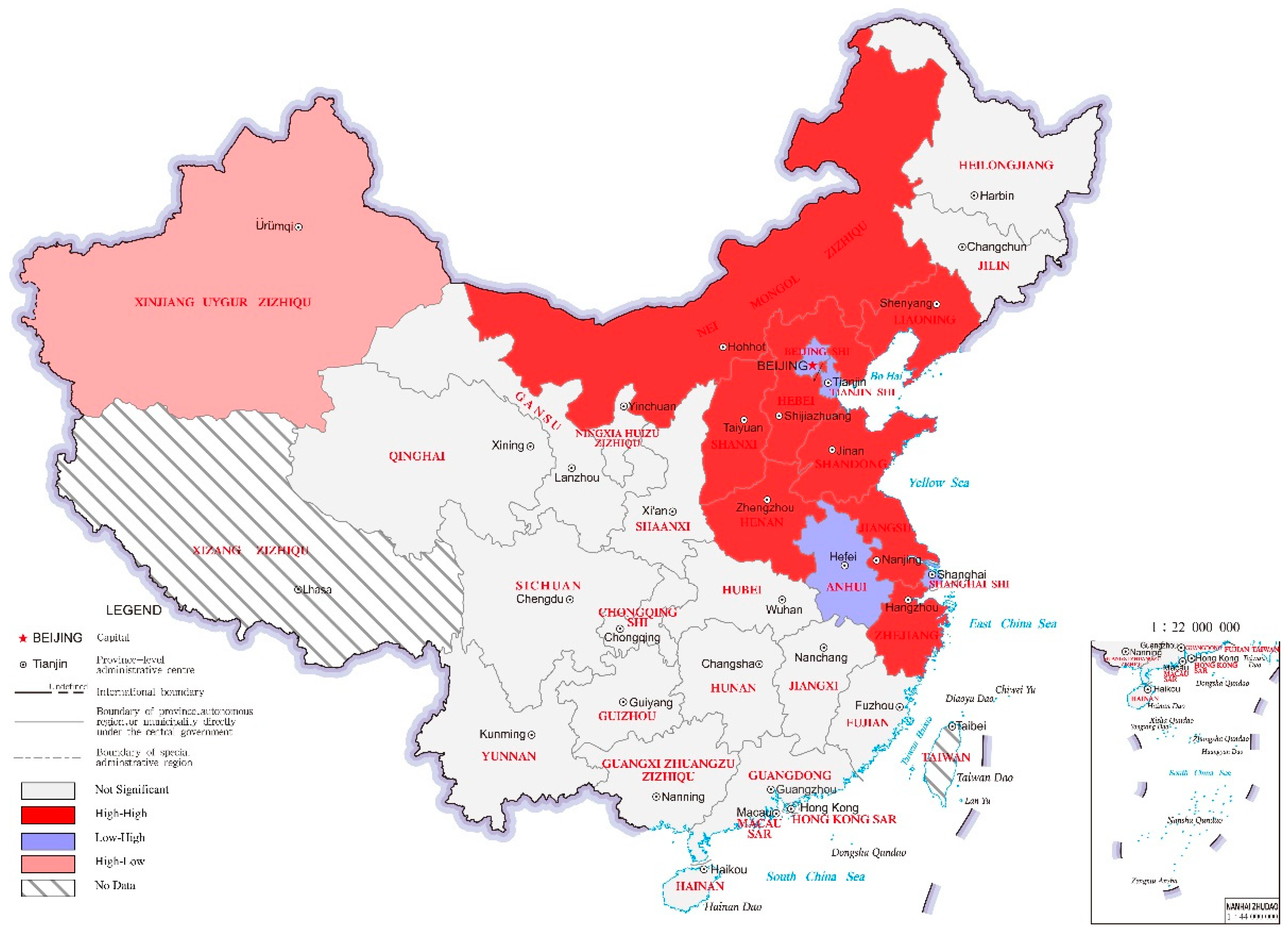
The spatial correlation of CO₂ emissions in China was calculated with Geoda 1.18 software using Formulas (2) and (3) (see Figure 4).

The results show that the global Moran’s I was 0.087, and the statistical significance test at 5% indicated that the spatial distribution of CO₂ emissions in each province was significantly positive; that is, the regions with high CO₂ emissions were relatively concentrated in terms of their locations. Shandong, Hebei, Henan, Shanxi, Liaoning, Jiangsu, Zhejiang, and Inner Mongolia were H-H agglomeration areas, indicating that local CO₂ emissions and those of neighbouring provinces were high. Beijing, Shanghai, Tianjin, and Anhui were L-H agglomeration areas, indicating that local CO₂ emissions were low and those of the surrounding provinces were high. Xinjiang was an H-L agglomeration area, indicating that local CO₂ emissions were high and those of the surrounding provinces were low.

The hotspots and coldspots of regional CO₂ emissions were plotted with ArcGIS 10.6 software using Formulas (4)–(6) (see Figure 5).

The results show that most of the hotspots were distributed in the eastern coastal areas. Liaoning and Inner Mongolia ranked highest, followed by the Beijing–Tianjin–Hebei and the Yangtze River Delta regions (Shanghai–Jiangsu–Zhejiang). Shandong, Shanxi, and Henan ranked in the central. Hainan, as an isolated province, was a coldspot for CO₂ emissions.

4.2. Measurement Model

4.2.1. Reliability Test

Reliability and construct validity are the keys to establishing the measurement model. Cronbach’s alpha, composite reliability (CR), and average variance extracted (AVE) were obtained using PLS algorithms [65].

Table 1. Factor loadings, Cronbach’s alpha, composite reliability (CR), and average variance extracted (AVE).

Latent Variables	Indicators	Factor Loading	t-Value	Cronbach’s Alpha	CR	AVE
Economic growth				0.847	0.899	0.747
EG1	GDP	0.864	81.788
EG2	Household consumption level	0.850	43.414
EG3	Per capita GDP	0.879	54.032
Industrial structure				0.968	0.984	0.969
IS1	Industrial added value as a percentage of GDP	0.986	375.863
IS2	Secondary industry as a percentage of GDP	0.983	297.067
Energy consumption				0.953	0.977	0.955
EC1	Electric energy production	0.975	345.139
EC2	Consumption of electric power	0.979	500.524
Urban development				0.948	0.967	0.906
UD1	Total fixed-asset investment	0.961	188.443
UD2	Urban employment	0.925	96.994
UD3	Number of civilian motor vehicles	0.968	235.794
Foreign trade				0.965	0.977	0.935
FT1	Number of foreign-invested enterprises	0.983	227.454
FT2	Total volume of foreign trade	0.970	285.679
FT3	Foreign direct investment	0.948	123.828
Government administration				0.975	0.984	0.953
GA1	Accepted number of domestic patent applications	0.987	413.46
GA2	Authorised number of domestic patent applications	0.986	273.979
GA3	Expenditures in science and technology of local government	0.956	105.985

Note: CR = composite reliability; AVE = average variance extracted.

shows all factor loadings of Cronbach’s alpha, CR, and AVE.

(1) Cronbach’s alpha was calculated to ensure composite reliability. By convention, Cronbach’s alpha should be greater or equal to 0.800 for a good scale and 0.700 for an acceptable scale. Table 1 shows that all Cronbach’s alpha values ranged from 0.899 to 0.984, which indicates that the measurement indexes had high reliability. (2) The CR was used to examine internal consistency. The higher the CR value, the higher the internal consistency of the plane; 0.700 is an acceptable threshold. We found the model to be sufficiently reliable and internally consistent, as shown in Table 1. (3) The AVE reflected the average commonality of each latent factor and was used to establish convergent validity. The AVE should be above 0.500 for all latent variables, whereby at least 50% of measurement variance is explained. Table 1 shows that all AVE values ranged from 0.747 to 0.969. In conclusion, the model had high reliability and construct validity, as evidenced by the verification of Cronbach’s alpha, CR, and AVE.

4.2.2. Validity Test

Convergent and discriminant validities were utilised to examine the model’s construct validity [65]. (1) Factor loading measures convergent validity and must be greater than 0.500. The factor loadings were greater than 0.850 (see Table 1), indicating that the measured variables had high convergence validity. (2) The square root of each construct’s AVE was greater than the bivariate correlation with the other constructs, which shows that the model had high convergent validity.

Table 2. Results of the hypothesis model.

Hypothesis	Path	Path Coefficient	t-Value	p-Value	95% BCa Confidence Intervals	f2	Support
H1	IS→CO2	0.122 ***	4.661	0.000	[0.080, 0.165]	0.048	Yes
H2	EC→CO2	0.995 ***	21.654	0.000	[0.916, 1.066]	0.858	Yes
H3	FT→CO2	−0.012	0.205	0.419	[−0.116, 0.107]	0.000	No
H4	GA→CO2	−0.528 ***	6.372	0.000	[−0.639, −0.380]	0.130	Yes
H5	UD→CO2	0.001	0.011	0.496	[−0.093, 0.102]	0.000	No
H6	EG→CO2	0.223 ***	4.013	0.000	[0.133, 0.307]	0.058	Yes
H7	IS→EG	−0.157 ***	4.651	0.000	[−0.229, −0.111]	0.068	Yes
H8	EC→EG	0.279 ***	4.311	0.000	[0.181, 0.399]	0.113	Yes
H9	FT→EG	0.302 ***	4.660	0.000	[0.200, 0.414]	0.068	Yes
H10	GA→EG	0.334 ***	3.270	0.001	[0.144, 0.472]	0.061	Yes

Note: BCa: bias corrected and accelerated bootstrap. Significance level: *** p < 0.001. EG = economic growth; IS = industrial structure; EC = energy consumption; UD = urban development; FT = foreign trade; GA = government administration.

shows the square roots of the AVEs and all the correlations. (3) The HTMT ratio is an important indicator used to evaluate discriminant validity by applying a PLS algorithm [66]. The HTMT ratio for the two latent variables was below 0.900. The HTMT values are shown in brackets in

Table 3. Discriminant validity.

	EG	IS	EC	UD	FT	GA
EG	0.865
IS	−0.083 (0.300)	0.984
EC	0.641 (0.599)	0.294 (0.305)	0.977
UD	0.695 (0.662)	0.177 (0.188)	0.864 (0.900)	0.952
FT	0.756 (0.796)	−0.012 (0.071)	0.586 (0.606)	0.566 (0.595)	0.967
GA	0.788 (0.809)	−0.007 (0.070)	0.689 (0.710)	0.771 (0.803)	0.873 (0.900)	0.976

Note: The square roots of AVEs are shown on the diagonal in bold. The HTMT ratios are in brackets. EG = economic growth; IS = industrial structure; EC = energy consumption; UD = urban development; FT = foreign trade; GA = government administration.

. In conclusion, the model has high convergent and discriminant validity, found through the verification of Cronbach’s alpha, CR, and AVE.

4.3. Structural Model

4.3.1. Path Coefficients and Significance

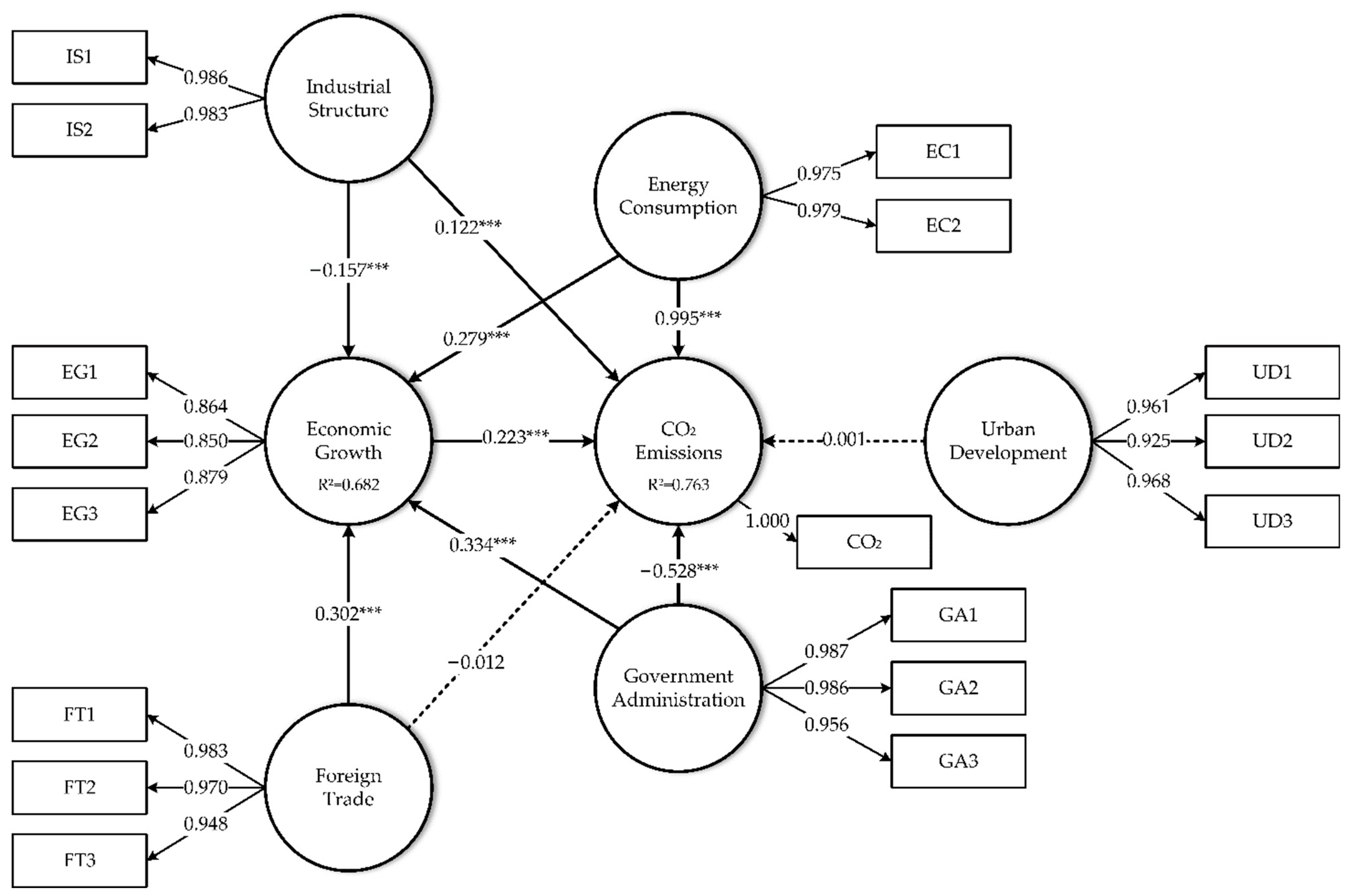
The bootstrapping method is a non-parametric statistical procedure that detects the statistical significance of various PLS-SEM results, including path coefficients, Cronbach’s alpha, HTMT, R² values, and the effect size f². Here, the number of sub-samples was set to 5000 and the t-test results were guaranteed to be significant at the level of 0.05 [65]. Table 2 shows the standardised path coefficients, t-values, and results. The results show that the path coefficients of the four latent variables (economic growth, industrial structure, energy consumption, and government administration) passed the significance test, and the four hypotheses were acceptable. This reveals that four factors had an impact on China’s total CO₂ emissions from 2006 to 2019. However, urban development and foreign trade did not pass the hypothesis test in this model, which does not mean that these two latent variables did not contribute to carbon emissions. On the contrary, these two variables had an impact on CO₂ emissions through the latent variable of economic growth. An f² above 0.02, 0.15, or 0.35 is considered a small, medium, or large effect, respectively. Additionally, the direct and indirect effects were analysed to verify the multiple mediation model (see Figure 6).

4.3.2. Direct, Indirect, Total, and Mediation Effects

Table 4. Results of direct, indirect, and mediating effects of economic growth.

Path	Direct Effect	Indirect Effect	t-Value	p-Value	95% Bca Confidence Intervals	Mediation Effect
IS→CO2	0.122 ***					Complementary (partial mediation)
IS→EG→CO2		−0.035 ***	3.313	0.000	[−0.054, −0.019]
EC→CO2	0.995 ***					Complementary (partial mediation)
EC→EG→CO2		0.060 ***	4.305	0.000	[0.400, 0.088]
FT→CO2	−0.012					Indirect-only (full mediation)
FT→EG→CO2		0.067 ***	3.114	0.001	[0.035, 0.103]
GA→CO2	−0.528 ***					Complementary (partial mediation)
GA→EG→CO2		0.077 *	1.955	0.025	[0.025, 0.138]

Note: Bca = bias corrected and accelerated bootstrap. Significance level: *** p < 0.001, * p < 0.05. IS = industrial structure; EC = energy consumption; FT = foreign trade; GA = government administration; UD = urban development; EG = economic growth; CO₂ = CO₂ emissions.

shows the direct, indirect, and total effects among latent variables and CO₂ emissions. Moreover, the positive effect of industrial structure on CO₂ emissions is more direct (0.122) than indirect (−0.035) through economic growth. The effect of energy consumption on CO₂ emissions is more direct (0.955) than indirect (0.060) through economic growth. The effect of foreign trade on CO₂ emissions is entirely indirect (0.067); the direct effect is not statistically significant. The effect of government administration on CO₂ emissions is also more direct (−0.528) than indirect (0.077).

Economic growth is a mediating variable of the effect of industrial structure, energy consumption, foreign trade, and government administration on CO₂ emissions. Therefore, H7, H8, H9, and H10 are supported. Table 4 shows the mediation effects of economic growth in the model.

4.3.3. Predictive Power

R² and Q² are important metrics for evaluating the predictability of a model. The R² value was obtained using a PLS calculation; Q² was calculated using blindfolding [65]. (1) The determination coefficient R² value was used as an indicator of the overall predictive strength of the model. Falk and Miller consider that R² value should be greater than 0.100 [67]; Chin [68] recommends 0.670, 0.330, and 0.100 (substantial, moderate, and weak, respectively); while Hair et al. [65] consider 0.750, 0.500, and 0.250 (substantial, moderate, and weak, respectively). The R² value (R² = 0.763 > 0.750) indicated that 76.3% of CO₂ emissions could be explained by the causality of six latent variables, showing that the model had substantial explanatory power. In addition, the R² value of economic growth was 0.682, indicating 68.2% of economic growth can be explained by industrial structure, energy consumption, foreign trade, and government administration. (2) The Stone–Geisser Q² value is a criterion for evaluating construct cross-validated redundancy. The larger the Q² value, the stronger the prediction correlation. The Q² value of CO₂ emissions was 0.754, indicating that the model had high predictive relevance.

4.4. Multigroup Analysis

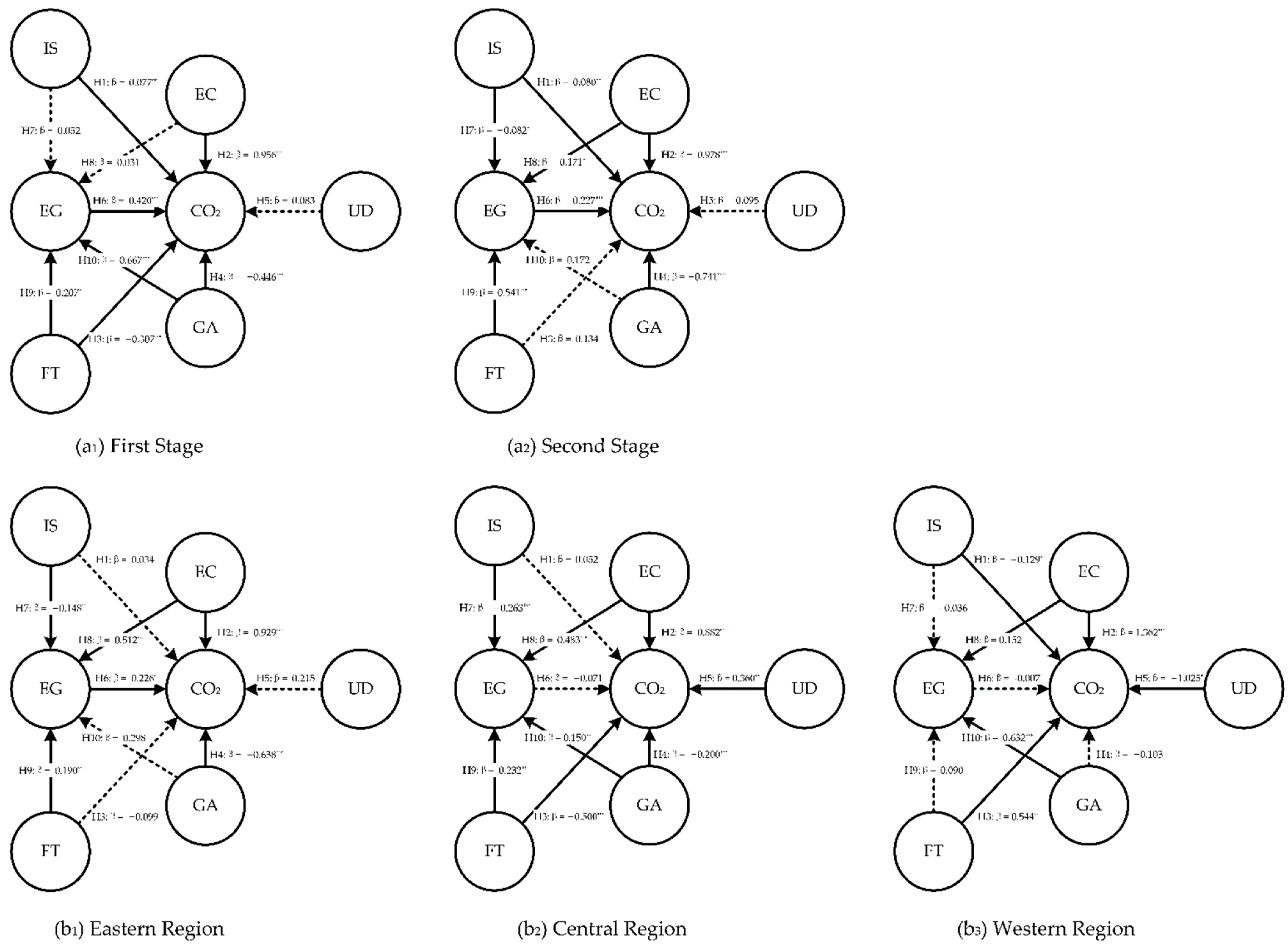
The PLS-MGA p-values revealed significant group differences in the MGA.

Table 5. Results of multigroup analysis on different periods and regions in China.

Part (A): First Stage (n = 180) vs. Second Stage (n = 240).
Hypothesis	Diff.	p-Value	Stage 1 (2006–2011)				Stage 2 (2012–2019)
			PC Mean	t-Value	p-Value	95% BCa CI	PC Mean	t-Value	p-Value	95% BCa CI
H1	−0.002	0.478	0.077 ***	2.475	0.007	[−0.028, 0.129]	0.080 **	2.421	0.008	[0.026, 0.132]
H2	−0.022	0.411	0.956 ***	9.454	0.000	[−0.797, 1.13]	0.978 ***	18.685	0.000	[0.888, 1.057]
H3	−0.449	0.001	−0.307 ***	3.216	0.001	[−0.499, −0.174]	0.134	1.172	0.121	[−0.029, 0.333]
H4	0.299	0.036	−0.446 ***	3.651	0.000	[−0.626, −0.252]	−0.741 ***	6.097	0.000	[−0.93, −0.545]
H5	−0.016	0.453	0.083	0.706	0.240	[−0.113, 0.237]	0.095	1.391	0.082	[−0.013, 0.2]
H6	0.201	0.025	0.420 ***	5.481	0.000	[−0.292, 0.54]	0.227 ***	3.432	0.000	[0.121, 0.327]
H7	0.134	0.029	0.052	0.923	0.178	[−0.045, 0.126]	−0.082 *	1.776	0.038	[−0.179, −0.016]
H8	−0.143	0.109	0.031	0.499	0.309	[−0.088, 0.172]	0.171 *	2.166	0.015	[0.055, 0.327]
H9	−0.314	0.011	0.207 *	2.139	0.016	[−0.049, 0.38]	0.541 ***	5.442	0.000	[0.381, 0.696]
H10	0.480	0.001	0.667 ***	6.046	0.000	[−0.466, 0.819]	0.172	1.325	0.093	[−0.065, 0.359]
Part (B): Eastern Region (n = 168) vs. Central Region (n = 140).
Hypothesis	Diff.	p-Value	Eastern Region				Central Region
			PC Mean	t-Value	p-Value	95% BCa CI	PC Mean	t-Value	p-Value	95% BCa CI
H1	−0.010	0.433	0.034	1.050	0.147	[−0.018, 0.102]	0.052	0.988	0.162	[−0.038, 0.126]
H2	0.016	0.469	0.929 ***	6.125	0.000	[0.656, 1.125]	0.882 ***	11.954	0.000	[0.765, 1.010]
H3	0.400	0.000	−0.099	1.026	0.152	[−0.225, 0.070]	−0.500 ***	6.346	0.000	[−0.613, −0.359]
H4	−0.424	0.001	−0.638 ***	5.434	0.000	[−0.812, −0.442]	−0.200 ***	3.639	0.000	[−0.287, −0.108]
H5	−0.110	0.309	0.215	1.542	0.062	[−0.004, 0.497]	0.360 **	2.348	0.009	[0.134, 0.610]
H6	0.278	0.009	0.226 *	2.144	0.016	[0.062, 0.365]	−0.071	0.949	0.171	[−0.196, 0.046]
H7	0.105	0.093	−0.148 **	2.839	0.002	[−0.273, −0.084]	−0.263 ***	4.874	0.000	[−0.353, −0.173]
H8	0.043	0.422	0.512 **	2.604	0.005	[0.227, 0.891]	0.483 ***	7.164	0.000	[0.368, 0.586]
H9	−0.037	0.378	0.190 **	2.460	0.007	[0.080, 0.339]	0.232 **	2.222	0.013	[0.045, 0.386]
H10	0.141	0.239	0.298	1.619	0.053	[−0.020, 0.567]	0.150 **	1.683	0.046	[0.015, 0.300]
Part (C): Eastern Region (n = 168) vs. Western Region (n = 112).
Hypothesis	Diff.	p-Value	Eastern Region				Western Region
			PC Mean	t-Value	p-Value	95% BCa CI	PC Mean	t-Value	p-Value	95% BCa CI
H1	0.161	0.01	0.034	2.148	0.147	[−0.016, 0.103]	−0.129 *	1.050	0.016	[−0.207, −0.020]
H2	−0.400	0.026	0.928 ***	8.889	0.000	[0.648, 1.132]	1.362 ***	6.033	0.000	[1.087, 1.541]
H3	−0.557	0.000	−0.098	2.651	0.152	[−0.224, 0.074]	0.544 **	1.027	0.004	[0.205, 0.719]
H4	−0.465	0.076	−0.637 ***	0.503	0.000	[−0.811, −0.440]	−0.103	5.459	0.307	[−0.655, 0.386]
H5	1.137	0.003	0.217	2.233	0.061	[0.004, 0.499]	−1.025 *	1.550	0.013	[−1.519, −0.183]
H6	0.164	0.163	0.225 *	0.329	0.013	[0.070, 0.360]	−0.007	2.222	0.371	[−0.198, 0.216]
H7	−0.119	0.071	−0.148 **	0.730	0.003	[−0.279, −0.086]	−0.036	2.803	0.233	[−0.152, 0.041]
H8	0.388	0.040	0.515 **	1.346	0.005	[0.218, 0.887]	0.152	2.583	0.089	[−0.021, 0.302]
H9	0.125	0.273	0.189 **	0.373	0.006	[0.080, 0.337]	0.090	2.488	0.355	[−0.281, 0.336]
H10	−0.367	0.068	0.296	3.831	0.051	[−0.021, 0.569]	0.632 ***	1.636	0.000	[0.396, 0.947]
Part (D): Central Region (n = 140) vs. Western Region (n = 112).
Hypothesis	Diff.	p-Value	Central Region				Western Region
			PC Mean	t-Value	p-Value	95% BCa CI	PC Mean	t-Value	p-Value	95% BCa CI
H1	0.171	0.013	0.053	2.126	0.166	[−0.042, 0.127]	−0.129 *	0.969	0.017	[−0.211, −0.025]
H2	−0.416	0.002	0.882 ***	9.022	0.000	[0.765, 1.007]	1.357 ***	11.907	0.000	[1.091, 1.543]
H3	−0.957	N.A.	−0.501 ***	2.680	0.000	[−0.604, −0.354]	0.542 **	6.403	0.004	[0.214, 0.719]
H4	−0.041	0.473	−0.200 ***	0.499	0.000	[−0.288, −0.106]	−0.118	3.614	0.309	[−0.655, 0.405]
H5	1.246	0.001	0.361 **	2.235	0.009	[0.121, 0.600]	−1.011 *	2.348	0.013	[−1.561, −0.245]
H6	−0.114	0.238	−0.070	0.332	0.171	[−0.199, 0.045]	−0.003	0.951	0.370	[−0.204, 0.211]
H7	−0.223	0.003	−0.262 ***	0.727	0.000	[−0.355, −0.176]	−0.035	4.848	0.234	[−0.147, 0.042]
H8	0.345	0.006	0.482 ***	1.333	0.000	[0.369, 0.592]	0.153	7.060	0.091	[−0.026, 0.301]
H9	0.162	0.223	0.230 *	0.372	0.013	[0.050, 0.390]	0.085	2.241	0.355	[−0.281, 0.328]
H10	−0.508	0.005	0.152 *	3.776	0.044	[0.009, 0.292]	0.634 ***	1.702	0.000	[0.388, 0.958]

Note: BCa CI = bias corrected and accelerated bootstrap confidence intervals. Significance level: * p < 0.05, ** p < 0.01, *** p < 0.001. Bold font: PLS-MGA p-value below 5% and above 95% indicate significant values. Diff. = path coefficient differences; PC = path coefficient; N.A. = not available. IS = industrial structure; EC = energy consumption; FT = foreign trade; GA = government administration; UD = urban development; EG = economic growth; CO₂ = CO₂ emissions.

and Figure 7 show the MGA for different regions and periods in China.

On the basis of the analysis of the temporal and spatial evolution characteristics of CO₂ emissions, we divided the study period into two control groups: 2006–2011 was the first growth stage, and 2012–2019 was the second growth stage. For the growth stage groups, H3, H4, and H6 differed significantly, showing that the impact of foreign trade, government administration, and economic growth on CO₂ emission for the first stage compared to the second stage group. Meanwhile, H7, H9, and H10 differed significantly, indicating that the impact of industrial structure, foreign trade, and government administration on economic growth in the first stage is stronger than in the second stage.

The pairwise comparison of the three regions in China revealed differences in the influencing factors of CO₂ emissions between the regions.

(1)

For the eastern and central groups, H3, H4, and H6 differed significantly, indicating that the impact of foreign trade, government administration, and economic growth on CO₂ emissions in the eastern region is stronger than in the central region.

(2)

For the eastern and western groups, H1, H2, H3, and H5 differed significantly, indicating that the impact of industrial structure, energy consumption, foreign trade, and urban development on CO₂ emissions in the eastern region is stronger than in the western region. Meanwhile, H8 differed significantly.

(3)

For the central and western groups, H1, H2, and H5 differed significantly, indicating that industrial structure, energy consumption, and urban development have stronger impacts on CO₂ emissions for the central than for the western region. Meanwhile, H7, H8, and H10 differed significantly. Likewise, we analysed the confidence intervals that allow us to verify if a path coefficient is significantly different from 0 as another way to assess the significance.

5. Discussion

5.1. Theoretical Implications

First, Figure 2, Figure 3 and Figure 4 show that spatio-temporal differences in China’s CO₂ emissions have a spatial scale effect. On the national scale, China’s total CO₂ emissions show a trend of gradual and steady growth. This is because China is in a period of rapid economic growth, and its CO₂ emissions are thus increasing rapidly. At the regional scale, the CO₂ emissions of the three main regions show decreasing distribution in the east, central, and west regions, which is consistent with the actual situation of China’s regional economic development [10]. At the provincial scale, provinces with high CO₂ emissions were mainly distributed in the eastern coastal region, indicating that provinces with high CO₂ emissions tend to be clustered together. Therefore, when formulating policies and development plans, the government should consider the spatial spillover effects of CO₂ emissions and the relevant influencing factors between neighbouring provinces.

Second, through confirmatory and structural model analyses, we found that the measurement model of the influencing factors for CO₂ emissions in China had high reliability and validity. Economic growth, industrial structure, energy consumption, and government management had a significant impact on carbon emissions. However, urbanisation development and foreign trade fail to pass the hypothesis test. These two latent variables had an impact on CO₂ emissions through the mediating effects of economic growth. The R² was 76.3%, and the Q² value was 75.4%, indicating that the structural equation model had a substantial explanatory and high predictive power.

Third, the path coefficients and significance of the six latent variables on CO₂ emissions were analysed. The results are as follows:

(1)

H1: Industrial structure contributes to more CO₂ emissions, which is consistent with the research results of Long et al. [69]. China is at the central stage of an industrialised economy; the development of secondary industries requires energy and resources. The proportion of secondary industries in China is larger than that of higher-income countries. Secondary industries have a high energy demand, and therefore their CO₂ emissions are also high.

(2)

H2: Energy consumption contributes to more CO₂ emissions, which is consistent with the results of Meng et al. [20]. With China’s economic development, the production and consumption of electric energy are growing, and the electric power industry has become the main sector of fossil fuel consumption and CO₂ emission. China’s energy consumption has always been based on coal; thermal power generation has long been the main component of power energy products, which will inevitably lead to the increase of CO₂ emissions.

(3)

H3: Foreign trade fails to pass the hypothesis test. With the acceleration of China’s integration into economic globalisation, China’s foreign trade volume increases, and a large number of foreign-funded enterprises enter into China, resulting in the rapid development of the local economy and thus contributing more CO₂ dioxide. This result supports hypothesis H9.

(4)

H4: Government administration contributes to reduced CO₂ emissions, which is consistent with the research results of Zheng et al. [70]. Government intervention reduces CO₂ emissions. The Chinese government can effectively reduce CO₂ emissions by implementing a variety of measures that are consistent with the national goal of energy conservation and emission reduction. Meanwhile, the government encourages enterprises to innovate independently and improve energy efficiency to reduce their CO₂ emissions. Therefore, the Chinese government has a restraining role in CO₂ emissions.

(5)

H5: Urban development fails to pass the hypothesis test. China is in a period of rapid urbanisation development, and the contribution of increased urbanisation to CO₂ emissions exists. As a matter of fact, with the influx of migrants into cities, the construction of infrastructure, such as buildings and transportation, is accelerating, which will bring about the rapid development of the urban economy and inevitably increase CO₂ emissions.

(6)

H6: Economic growth has a positive impact on CO₂ emissions, which is consistent with the findings of Cui et al. [16] and Li et al. [71]. China is currently at the central stage of economic development and undergoing large-scale economic growth and rapid development. Therefore, energy consumption and CO₂ emissions are high. This is consistent with the spatio-temporal evolution pattern of China’s CO₂ emissions.

Economic growth is an important intervening variable in the model. The mediation of economic growth is complementary (partial mediation) between industrial structure and CO₂ emissions; the mediation of economic growth is complementary (partial mediation) between energy consumption and CO₂ emissions; the mediation of economic growth is indirect-only (full mediation) between foreign trade and CO₂ emissions; the mediation of economic growth is complementary (partial mediation) between government administration and CO₂ emissions. These results are consistent with China’s multiple goals of pursuing both environmental protection and economic and social progress.

Fourth, through the MGA of different stages and regions, we found differences in the effect intensity of different influencing factors on CO₂ emissions at different development stages and different regions. Compared with the second stage, the impact of foreign trade, government administration, and economic growth on CO₂ emissions in the first stage was significantly different. This is because of China’s accession to the World Trade Organization in the early 21st century, which significantly accelerated China’s participation in economic globalisation and opening-up and increased its import and export trade. During the 11th Five-Year Plan period (2006–2010), the central government promulgated the implementation of energy-saving target responsibility and evaluation, which has achieved some results. Progress has also been made toward the overall goal of building a resource-conserving and environment-friendly society, as proposed in the 12th Five-Year Plan (2011–2015) and 13th Five-Year Plan (2016–2020).

Fifth, through an MGA of different regions, we found differences in the effect intensity of various influencing factors on CO₂ emissions in different regions; this result is consistent with the current state of China’s regional economic development [46].

(1)

The impact of foreign trade (H3), government administration (H4), and economic growth (H6) on CO₂ emissions in the eastern region was stronger than that in the central region. The eastern coastal region took the lead in implementing the reform and opening-up strategy, and its economy started early and developed rapidly. In addition, the eastern region is a densely populated urban area of China; as such, it is also the core region for CO₂ emissions. In recent years, the eastern region has taken the lead in implementing the energy conservation and emission reduction strategy. For example, the CO₂ emissions for Beijing showed negative growth, while those for Shanghai and Tianjin showed low growth.

(2)

The impact of industrial structure (H1), energy consumption (H2), foreign trade (H3), and urban development (H5) on CO₂ emissions in the eastern region was stronger than in the western region. Compared with the eastern region, there is a huge gap in economic development, industrial structure, and urban development in the western region, which is also consistent with the actual situation of China’s regional development. The western region is a relatively backward region regarding economic development and has lower CO₂ emissions than the eastern and central regions. However, with the implementation of development and the opening-up strategy in recent years, emissions in the western region have rapidly increased, especially in Ningxia and Xinjiang, where the growth rates of CO₂ emissions are among the highest in the entire country. The current development in the western region still follows the model for inefficient, blind, and energy-intensive development; thus, the growth rate of CO₂ emissions is accelerating. Additionally, the western region is a key and difficult area in China’s ecological construction due to its vast territory and fragile environment. Overall, CO₂ emissions in the west are problematic.

(3)

The impacts of industrial structure (H1), energy consumption (H2), and urban development (H5) on CO₂ emissions in the central region were stronger than that in the western region. The central region is the main energy- and resource-producing area in China, and its industrial structure is dominated by secondary industries. Faced with prosperity in the east and development in the west, the central region has experienced economic collapse. In recent years, the central region has taken over industries with excess capacity from the east, and the rise of urban clusters has led to continuous CO₂ emissions.

5.2. Practical Implications

Given the above analysis, China’s energy conservation and emission reduction measures can be proposed in six dimensions.

• China should improve the quality of economic growth through industrial upgrading, energy restructuring, and technological progress to change the economic growth model; it should also realise an extensive development model to intensify development model change.
• Per the law of industrial structure development at the present stage, China should strive to develop tertiary industries, promote the upgrading of secondary industries, advocate a circular economy, and encourage the development of green and environmental protection industries.
• China should continue to increase the proportion of clean energy in energy consumption; develop clean energy, such as wind power, solar energy, hydropower, and nuclear energy; and develop clean energy technologies and improve energy efficiency.
• China should remain on the path of green urbanisation and raise people’s awareness about green consumption.
• The Chinese government should formulate a strict environmental access system, improve environment-related rules and regulations, and control high pollution and high energy consumption projects.
• The government has increased investment in science and technology and environmental protection and has adopted preferential policies to encourage local enterprises to engage in independent innovation.
• Energy conservation and emission reductions are gradual processes that should be based on actual economic growth stages and regional patterns to promote the transformation and sustainable development of different regions.

6. Conclusions

This study analysed the spatial and temporal pattern of CO₂ emissions in China and clarified the determinants of CO₂ emissions and their internal relationships. First, six driving factors that affect CO₂ emissions were clarified, including economic growth, industrial structure, energy consumption, urban development, foreign trade, and government management, and a conceptual model was constructed. Second, mathematical statistics, spatial autocorrelation, and hotspot analysis were used to analyse the spatial and temporal patterns of CO₂ emissions in China. Third, the reliability, validity, path coefficient, and prediction ability of the structural equation model for CO₂ emissions were tested using 420 samples from 30 provinces in China during 14 years from 2006 to 2019. Fourth, multigroup analysis was used to analyse the differences between the impact paths of different regions and stages. Finally, we propose targeted policy suggestions for China’s future CO₂ emission reduction to provide a reference for achieving the goals of peak carbon and carbon neutrality. The main conclusions are as follows:

First, China’s CO₂ emissions have different spatial and temporal patterns. On the national scale, China’s total CO₂ emissions show a trend of gradual and steady growth. At the regional scale, the CO₂ emissions of the three main regions show a decreasing distribution pattern of east, central, and west. At the provincial scale, the eastern coastal area is a hotspot for high CO₂ emissions. These results are consistent with the actual status of China’s regional economic development.

Second, this study constructed a structural equation model on drivers of CO₂ emissions, including economic growth, industrial structure, energy consumption, urban development, foreign trade, and government management. The conceptual model was tested with 420 samples from 30 provinces in China from 2006 to 2019. We found that the R² value was 76.3% and the Q² value was 75.4%, indicating that the proposed model had a substantial explanatory power and a high predictive power.

Third, through path coefficient analysis and hypothesis testing, we found that latent variables had different degrees of influence on CO₂ emissions. As China’s secondary industries still occupy an important position in GDP and consume a large amount of energy, the industrial structure contributes to more CO₂ emissions. Because coal has always been the main energy consumption in China, electricity consumption and production burn a large amount of fossil fuel and emit a large amount of CO₂. Therefore, energy consumption contributes to higher CO₂ emissions. Government administration can effectively control CO₂ emissions through positive and effective measures. Foreign trade does not pass the hypothesis test but has an impact on CO₂ emissions through the mediating role of economic growth. Urban development does not pass the hypothesis test, but China’s urbanisation is an important factor that cannot be ignored. As China’s current economic development is still on the rise, the impact of economic growth on CO₂ emissions is significantly positive. Meanwhile, economic growth is a mediating variable of the impact of industrial structure, energy consumption, foreign trade, and government administration on CO₂ emissions.

Fourth, through the calculation of the MGA methods, we found that latent variables in different development stages and regions have different effects on CO₂ emissions. By comparing the two development stages, we found significant differences in the impact of foreign trade, government administration, and economic growth on CO₂ emissions. This is consistent with the extent of China’s reform and opening-up and the government’s concept and practice of green development. Through a comparison of the three main regions, we found that the impact of foreign trade, government administration, and economic growth on CO₂ emissions in the eastern region was stronger than that in the central region; the impact of industrial structure, energy consumption, foreign trade, and urban development on CO₂ emissions in the eastern region was stronger than that in the western region; and the impact of industrial structure, energy consumption, and urban development on CO₂ emissions in the central region was stronger than that in the western region. These calculation results are consistent with the actual situation of China’s regional economic development.

There are some limitations in this paper, and further research suggestions are proposed. First, the factors that affect CO₂ emissions are diverse, and more latent variables should be considered, such as renewable energy production, macro-control policies, technological progress, and residents’ consumption awareness. Second, the selection of indicators has an impact on the intensity of CO₂ emissions, and therefore other indicators should be considered in the future. Third, more causal relationships between latent variables and their mediating effects should be explored in depth.

References

- Sachs, J.D.; Schmidt-Traub, G.; Mazzucato, M.; Messner, D.; Nakicenovic, N.; Rockström, J. Six transformations to achieve the sustainable development goals. Nat. Sustain. 2019, 2, 805–814. [Google Scholar] [CrossRef]
- Baruch-Mordo, S.; Kiesecker, J.M.; Kennedy, C.M.; Oakleaf, J.R.; Opperman, J.J. From Paris to practice: Sustainable implementation of renewable energy goals. Environ. Res. Lett. 2018, 14, 024013. [Google Scholar] [CrossRef]
- Kokotovic, F.; Kurecic, P.; Mjeda, T. Accomplishing the sustainable development goal 13—Climate action and the role of the European Union. Interdiscip. Descr. Complex Syst. 2019, 17, 132–145. [Google Scholar] [CrossRef]
- Yang, L.; Li, Y. Low-carbon city in China. Sustain. Cities Soc. 2013, 9, 62–66. [Google Scholar] [CrossRef]
- He, J. Global low-carbon transition and China’s response strategies. Adv. Clim. Chang. Res. 2016, 7, 204–212. [Google Scholar] [CrossRef]
- He, J.; Yu, Z.; Zhang, D. China’s strategy for energy development and climate change mitigation. Energy Policy 2012, 51, 7–13. [Google Scholar]
- He, J. Situation and measures of China’s CO2 emission mitigation after the Paris agreement. Front. Energy 2018, 12, 353–361. [Google Scholar] [CrossRef]
- Kuhn, B.M. China’s commitment to the sustainable development goals: An analysis of push and pull factors and implementation challenges. Chin. Political Sci. Rev. 2018, 3, 359–388. [Google Scholar] [CrossRef]
- Yang, S.; Zhao, D.; Wu, Y.; Fan, J. Regional variation in carbon emissions and its driving forces in China: An index decomposition analysis. Energy Environ. 2013, 24, 1249–1270. [Google Scholar] [CrossRef] [Green Version]
- Wang, Y.; Zheng, Y. Spatial effects of carbon emission intensity and regional development in China. Environ. Sci. Pollut. Res. 2021, 28, 14131–14143. [Google Scholar] [CrossRef]
- Sun, L.; Wu, L.; Qi, P. Global characteristics and trends of research on industrial structure and carbon emissions: A bibliometric analysis. Environ. Sci. Pollut. Res. 2020, 27, 44892–44905. [Google Scholar] [CrossRef]
- Guo, F.; Meng, S.; Sun, R. The evolution characteristics and influence factors of carbon productivity in China’s industrial sector: From the perspective of embodied carbon emissions. Environ. Sci. Pollut. Res. 2021, 28, 50611–50622. [Google Scholar] [CrossRef]
- Zheng, H.; Gao, X.; Sun, Q.; Han, X.; Wang, Z. The impact of regional industrial structure differences on carbon emission differences in China: An evolutionary perspective. J. Clean. Prod. 2020, 257, 120506. [Google Scholar] [CrossRef]
- Li, L.; Hong, X.; Peng, K. A spatial panel analysis of carbon emissions, economic growth and high-technology industry in China. Struct. Chang. Econ. Dyn. 2019, 49, 83–92. [Google Scholar] [CrossRef]
- Zhou, D.; Zhang, X.; Wang, X. Research on coupling degree and coupling path between China’s carbon emission efficiency and industrial structure upgrading. Environ. Sci. Pollut. Res. 2020, 27, 25149–25162. [Google Scholar] [CrossRef] [PubMed]
- Cui, E.; Ren, L.; Sun, H. Analysis on the regional difference and impact factors of CO2 emissions in China. Environ. Prog. Sustain. Energy 2017, 36, 1282–1289. [Google Scholar] [CrossRef]
- Wang, D.; Liu, X.; Yang, X.; Zhang, Z.; Wen, X.; Zhao, Y. China’s energy transition policy expectation and its CO2 emission reduction effect assessment. Front. Energy Res. 2021, 8, 8. [Google Scholar] [CrossRef]
- Wang, S.; Wang, J.; Li, S.; Fang, C.; Feng, K. Socioeconomic driving forces and scenario simulation of CO2 emissions for a fast-developing region in China. J. Clean. Prod. 2019, 216, 217–229. [Google Scholar] [CrossRef]
- Xu, B.; Zhong, R.; Hochman, G.; Dong, K. The environmental consequences of fossil fuels in China: National and regional perspectives. Sustain. Dev. 2019, 27, 826–837. [Google Scholar] [CrossRef]
- Meng, M.; Jing, K.; Mander, S. Scenario analysis of CO2 emissions from China’s electric power industry. J. Clean. Prod. 2017, 142, 3101–3108. [Google Scholar] [CrossRef]
- Wang, S.; Wang, X.; Tang, Y. Drivers of carbon emission transfer in China—An analysis of international trade from 2004 to 2011. Sci. Total Environ. 2020, 709, 135924. [Google Scholar] [CrossRef]
- Zhang, L.; Xiong, L.; Cheng, B.; Yu, C. How does foreign trade influence China’s carbon productivity? Based on panel spatial lag model analysis. Struct. Chang. Econ. Dyn. 2018, 47, 171–179. [Google Scholar] [CrossRef]
- Chen, Y.; Wang, Z.; Zhong, Z. CO2 emissions, economic growth, renewable and non-renewable energy production and foreign trade in China. Renew. Energy 2019, 131, 208–216. [Google Scholar] [CrossRef]
- Tan, S.; Zhang, M.; Wang, A.; Zhang, X.; Chen, T. How do varying socio-economic driving forces affect China’s carbon emissions? New evidence from a multiscale geographically weighted regression model. Environ. Sci. Pollut. Res. 2021, 28, 41242–41254. [Google Scholar] [CrossRef]
- Jiang, M.; An, H.; Gao, X.; Liu, S.; Xi, X. Factors driving global carbon emissions: A complex network perspective. Resour. Conserv. Recycl. 2019, 146, 431–440. [Google Scholar] [CrossRef]
- Cao, Z.; Wei, J. Industrial distribution and LMDI decomposition of trade-embodied CO2 in China. Dev. Econ. 2019, 57, 211–232. [Google Scholar] [CrossRef]
- Pan, X.; Pan, X.; Li, C.; Song, J.; Zhang, J. Effects of China’s environmental policy on carbon emission efficiency. Int. J. Clim. Chang. Strat. Manag. 2019, 11, 326–340. [Google Scholar] [CrossRef] [Green Version]
- He, L.; Yin, F.; Zhong, Z.; Ding, Z. The impact of local government investment on the carbon emissions reduction effect: An empirical analysis of panel data from 30 provinces and municipalities in China. PLoS ONE 2017, 12, e0180946. [Google Scholar] [CrossRef] [PubMed] [Green Version]
- Lin, B.; Jia, Z. The energy, environmental and economic impacts of carbon tax rate and taxation industry: A CGE based study in China. Energy 2018, 159, 558–568. [Google Scholar] [CrossRef]
- Zhang, F.; Jin, G.; Li, J.; Wang, C.; Xu, N. Study on dynamic total factor carbon emission efficiency in China’s urban agglomerations. Sustainability 2020, 12, 2675. [Google Scholar] [CrossRef] [Green Version]
- Sun, W.; Huang, C. How does urbanization affect carbon emission efficiency? Evidence from China. J. Clean. Prod. 2020, 272, 122828. [Google Scholar] [CrossRef]
- Zhou, C.; Wang, S.; Wang, J. Examining the influences of urbanization on carbon dioxide emissions in the Yangtze River Delta, China: Kuznets curve relationship. Sci. Total Environ. 2019, 675, 472–482. [Google Scholar] [CrossRef]
- Han, X.; Cao, T.; Sun, T. Analysis on the variation rule and influencing factors of energy consumption carbon emission intensity in China’s urbanization construction. J. Clean. Prod. 2019, 238, 117958. [Google Scholar] [CrossRef]
- Xu, L.; Du, H.; Zhang, X. Driving forces of carbon dioxide emissions in China’s cities: An empirical analysis based on the geodetector method. J. Clean. Prod. 2021, 287, 125169. [Google Scholar] [CrossRef]
- Dinda, S. Environmental kuznets curve hypothesis: A survey. Ecol. Econ. 2004, 49, 431–455. [Google Scholar] [CrossRef] [Green Version]
- Fang, D.; Hao, P.; Wang, Z.; Hao, J. Analysis of the influence mechanism of CO2 emissions and verification of the environmental kuznets curve in China. Int. J. Environ. Res. Public Health 2019, 16, 944. [Google Scholar] [CrossRef] [Green Version]
- Mardani, A.; Streimikiene, D.; Cavallaro, F.; Loganathan, N.; Khoshnoudi, M. Carbon dioxide (CO2) emissions and economic growth: A systematic review of two decades of research from 1995 to 2017. Sci. Total Environ. 2019, 649, 31–49. [Google Scholar] [CrossRef] [PubMed]
- Duro, J.A.; Padilla, E. International inequalities in per capita CO2 emissions: A decomposition methodology by Kaya factors. Energy Econ. 2006, 28, 170–187. [Google Scholar] [CrossRef]
- Yuan, J.; Xu, Y.; Hu, Z.; Zhao, C.; Xiong, M.; Guo, J. Peak energy consumption and CO2 emissions in China. Energy Policy 2014, 68, 508–523. [Google Scholar] [CrossRef]
- Green, F.; Stern, N. China’s changing economy: Implications for its carbon dioxide emissions. Clim. Policy 2017, 17, 423–442. [Google Scholar] [CrossRef] [Green Version]
- Dietz, T.; Rosa, E.A. Effects of population and affluence on CO2 emissions. Proc. Natl. Acad. Sci. USA 1997, 94, 175–179. [Google Scholar] [CrossRef] [PubMed] [Green Version]
- Feng, K.; Hubacek, K.; Guan, D. Lifestyles, technology and CO2 emissions in China: A regional comparative analysis. Ecol. Econ. 2009, 69, 145–154. [Google Scholar] [CrossRef]
- Wang, C.; Wang, F.; Zhang, X.; Yang, Y.; Su, Y.; Ye, Y.; Zhang, H. Examining the driving factors of energy related carbon emissions using the extended STIRPAT model based on IPAT identity in Xinjiang. Renew. Sustain. Energy Rev. 2017, 67, 51–61. [Google Scholar] [CrossRef]
- Wang, C.; Chen, J.; Zou, J. Decomposition of energy-related CO2 emission in China: 1957–2000. Energy 2005, 30, 73–83. [Google Scholar] [CrossRef]
- Hatzigeorgiou, E.; Polatidis, H.; Haralambopoulos, D. CO2 emissions in Greece for 1990–2002: A decomposition analysis and comparison of results using the arithmetic mean divisia index and logarithmic mean divisia index techniques. Energy 2008, 33, 492–499. [Google Scholar] [CrossRef]
- Xu, S.-C.; He, Z.-X.; Long, R.-Y. Factors that influence carbon emissions due to energy consumption in China: Decomposition analysis using LMDI. Appl. Energy 2014, 127, 182–193. [Google Scholar] [CrossRef]
- Shao, S.; Yang, L.; Gan, C.; Cao, J.; Geng, Y.; Guan, D. Using an extended LMDI model to explore techno-economic drivers of energy-related industrial CO2 emission changes: A case study for Shanghai (China). Renew. Sustain. Energy Rev. 2016, 55, 516–536. [Google Scholar] [CrossRef] [Green Version]
- Zheng, H.; Hu, J.; Guan, R.; Wang, S. Examining determinants of CO2 emissions in 73 cities in China. Sustainability 2016, 8, 1296. [Google Scholar] [CrossRef]
- Li, W.; Wang, W.; Wang, Y.; Qin, Y. Industrial structure, technological progress and CO2 emissions in China: Analysis based on the STIRPAT framework. Nat. Hazards 2017, 88, 1545–1564. [Google Scholar] [CrossRef]
- Zheng, D.C.; Liu, W.X.; Li, X.X.; Lin, Z.Y.; Jiang, H. Research on carbon emission diversity from the perspective of urbanization. Appl. Ecol. Environ. Res. 2018, 16, 6643–6654. [Google Scholar] [CrossRef]
- Chen, J.; Lian, X.; Su, H.; Zhang, Z.; Ma, X.; Chang, B. Analysis of China’s carbon emission driving factors based on the perspective of eight major economic regions. Environ. Sci. Pollut. Res. 2021, 28, 8181–8204. [Google Scholar] [CrossRef]
- Li, J.; Cheng, J.; Diao, B.; Wu, Y.; Hu, P.; Jiang, S. Social and economic factors of industrial carbon dioxide in China: From the perspective of spatiotemporal transition. Sustainability 2021, 13, 4268. [Google Scholar] [CrossRef]
- Sha, W.; Chen, Y.; Wu, J.; Wang, Z. Will polycentric cities cause more CO2 emissions? A case study of 232 Chinese cities. J. Environ. Sci. 2020, 96, 33–43. [Google Scholar] [CrossRef]
- Chen, J.; Wang, L.; Li, Y. Research on the impact of multi-dimensional urbanization on China’s carbon emissions under the background of COP21. J. Environ. Manag. 2020, 273, 111123. [Google Scholar] [CrossRef] [PubMed]
- Sun, Z.-Q.; Sun, T. The impact of multi-dimensional urbanization on China’s carbon emissions based on the spatial spillover effect. Pol. J. Environ. Stud. 2020, 29, 3317–3327. [Google Scholar] [CrossRef]
- Zhang, X.; Zhao, Y. Identification of the driving factors’ influences on regional energy-related carbon emissions in China based on geographical detector method. Environ. Sci. Pollut. Res. 2018, 25, 9626–9635. [Google Scholar] [CrossRef] [PubMed]
- Sarstedt, M.; Cheah, J.-H. Partial least squares structural equation modeling using SmartPLS: A software review. J. Mark. Anal. 2019, 7, 196–202. [Google Scholar] [CrossRef]
- Ben Jabeur, S.; Sghaier, A. The relationship between energy, pollution, economic growth and corruption: A partial least squares structural equation modeling (PLS-SEM) Approach. Econ. Bull. 2018, 38, 1927–1946. [Google Scholar]
- Wei, Y.; Zhu, X.; Li, Y.; Yao, T.; Tao, Y. Influential factors of national and regional CO2 emission in China based on combined model of DPSIR and PLS-SEM. J. Clean. Prod. 2019, 212, 698–712. [Google Scholar] [CrossRef]
- Soltani, M.; Rahmani, O.; Ghasimi, D.S.; Ghaderpour, Y.; Pour, A.B.; Misnan, S.H.; Ngah, I. Impact of household demographic characteristics on energy conservation and carbon dioxide emission: Case from Mahabad city, Iran. Energy 2020, 194, 116916. [Google Scholar] [CrossRef]
- Li, W.; Zhao, S.; Ma, J.; Qin, W. Investigating regional and generational heterogeneity in low-carbon travel behavior intention based on a PLS-SEM approach. Sustainability 2021, 13, 3492. [Google Scholar] [CrossRef]
- Wang, B.; Li, J.; Sun, A.; Wang, Y.; Wu, D. Residents’ green purchasing intentions in a developing-country context: Integrating PLS-SEM and MGA methods. Sustainability 2019, 12, 30. [Google Scholar] [CrossRef] [Green Version]
- Luo, L.; Qian, T.Y.; Rich, G.; Zhang, J.J. Impact of market demand on recurring hallmark sporting event spectators: An empirical study of the Shanghai Masters. Int. J. Sports Mark. Spons. 2021. [Google Scholar] [CrossRef]
- Schirmer, N.; Ringle, C.M.; Gudergan, S.P.; Feistel, M.S.G. The link between customer satisfaction and loyalty: The moderating role of customer characteristics. J. Strateg. Mark. 2018, 26, 298–317. [Google Scholar] [CrossRef]
- Hair, J.F.; Hult, G.T.M.; Ringle, C.M.; Sarstedt, M. A Primer on Partial Least Squares Structural Equation Modeling (PLS-SEM), 3rd ed.; Sage Publications: Thousand Oaks, CA, USA, 2021. [Google Scholar]
- Henseler, J.; Ringle, C.M.; Sarstedt, M. A new criterion for assessing discriminant validity in variance-based structural equation modeling. J. Acad. Mark. Sci. 2015, 43, 115–135. [Google Scholar] [CrossRef] [Green Version]
- Falk, R.F.; Miller, N.B. A Primer for Soft Modeling; University of Akron Press: Akron, OH, USA, 1992. [Google Scholar]
- Chin, W.W. The partial least squares approach to structural equation modeling. Mod. Methods Bus. Res. 1998, 295, 295–336. [Google Scholar]
- Long, R.; Shao, T.; Chen, H. Spatial econometric analysis of China’s province-level industrial carbon productivity and its influencing factors. Appl. Energy 2016, 166, 210–219. [Google Scholar] [CrossRef]
- Zeng, L.; Lu, H.; Liu, Y.; Zhou, Y.; Hu, H. Analysis of regional differences and influencing factors on China’s carbon emission efficiency in 2005–2015. Energies 2019, 12, 3081. [Google Scholar] [CrossRef] [Green Version]
- Li, R.; Wang, Q.; Liu, Y.; Jiang, R. Per-capita carbon emissions in 147 countries: The effect of economic, energy, social, and trade structural changes. Sustain. Prod. Consum. 2021, 27, 1149–1164. [Google Scholar] [CrossRef]
Figure 1.
Proposed conceptual model.
Figure 2.
Averages of CO2 emissions in three main regions in China from 2006 to 2019.
Figure 3.
CO2 emissions for 30 provinces in China from 2006 to 2019.
Figure 4.
Local autocorrelation of CO2 emissions in China from 2006 to 2019.
Figure 5.
Hotspots of CO2 emissions in China from 2006 to 2019.
Figure 6.
Results of PLS-SEM. Note: The dotted line indicates that the path fails the hypothesis test, and the solid line indicates that the path passes the hypothesis test. *** p < 0.001.
Figure 7.
MGA of different periods and regions. Note: The dotted line indicates that the path fails the hypothesis test, and the solid line indicates that the path passes the hypothesis test. * < 0.05; p ** p < 0.01; *** p < 0.001. IS = industrial structure; EC = energy consumption; FT = foreign trade; GA = government administration; UD = urban development; EG = economic growth; CO2 = CO2 emissions.