
Optimization of Sliding Mode Control to Save Energy in a SCARA Robot


 , ,
, ,  ,
,  and
and
Abstract
:1. Introduction
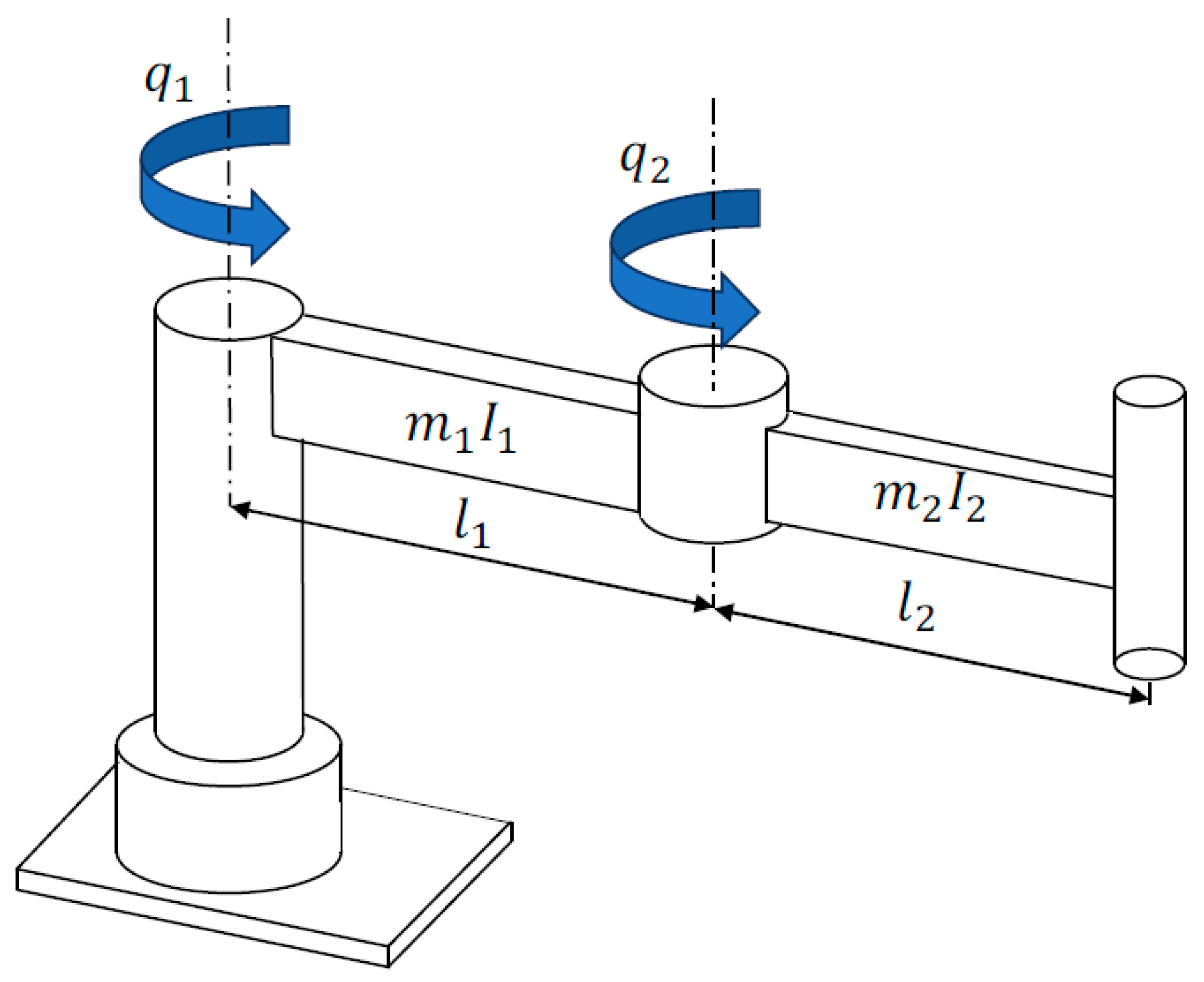
2. Dynamic Model of a Two-DOF SCARA Robot
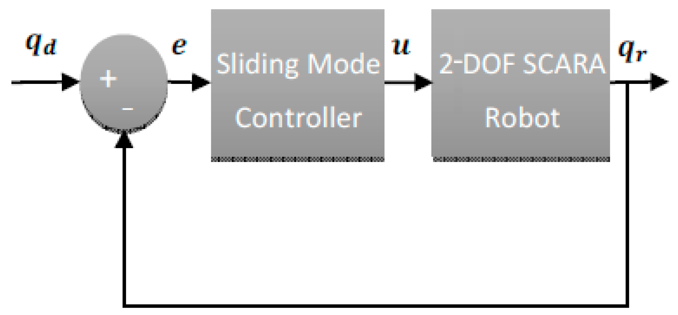
3. Sliding Mode Controller Design
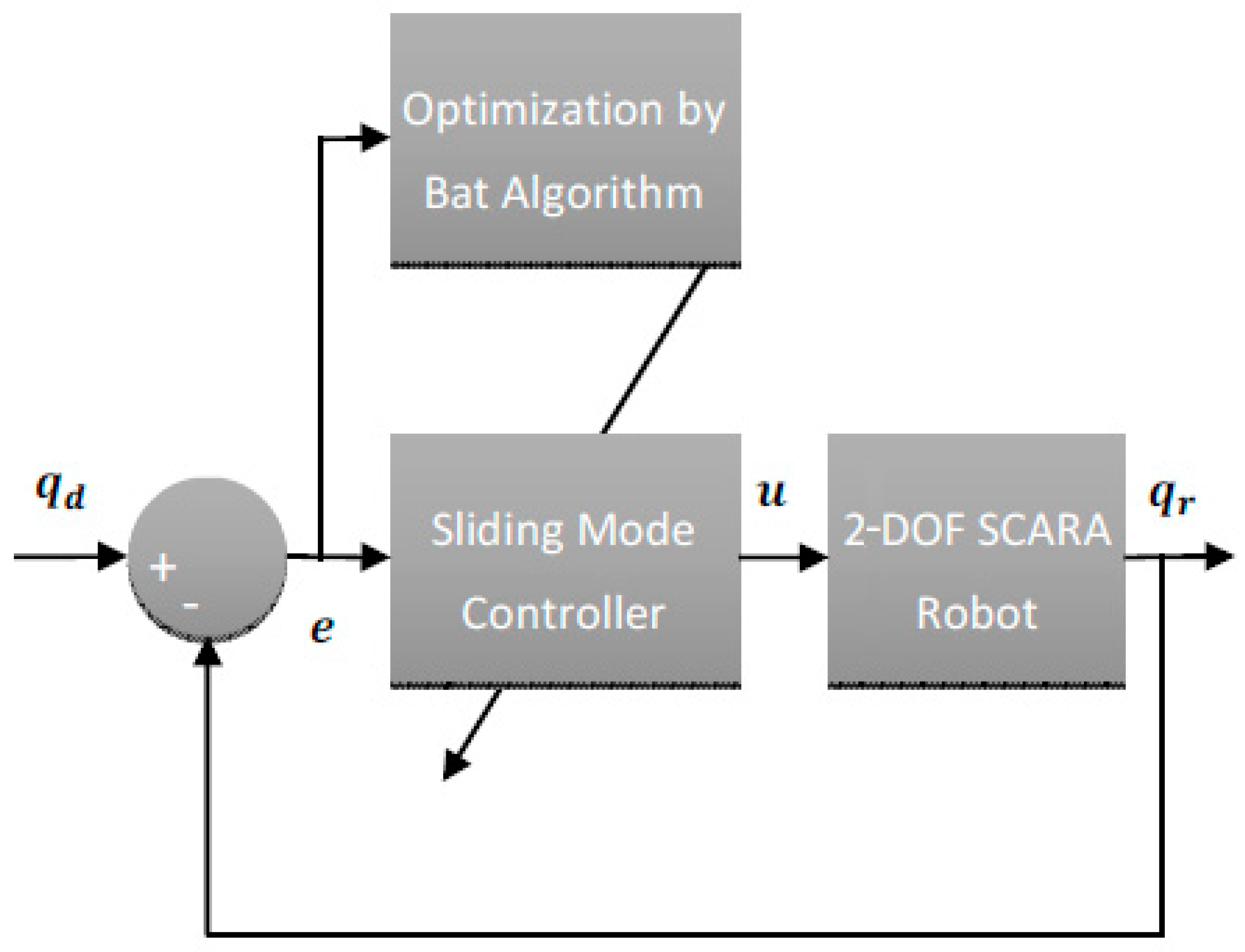
4. Optimization of SMC Using the Bat Algorithm
- Generate the bat population and initial velocity , = (1, 2).
- Define the pulse frequency in .
- Initialize the values for the pulse rate and loudness .
- While ( < maximum iteration number):
- Update frequency () and velocity () according to Equations (28) and (30), respectively.
- If ():
- Update position () according to Equation (31).
- Otherwise, update position () according to Equations (29), (32), and (33).
- End If.
- Determine the target functions and for with Equations (37)–(39) or determine the target functions and for with Equations (40)–(42).
- If ():
- Accept the new result with Equation (34).
- Decrease and increase according to Equations (35) and (36), respectively.
- End If
- If () or If ():
- Accept the past value of with Equation (43) or (44).
- End If
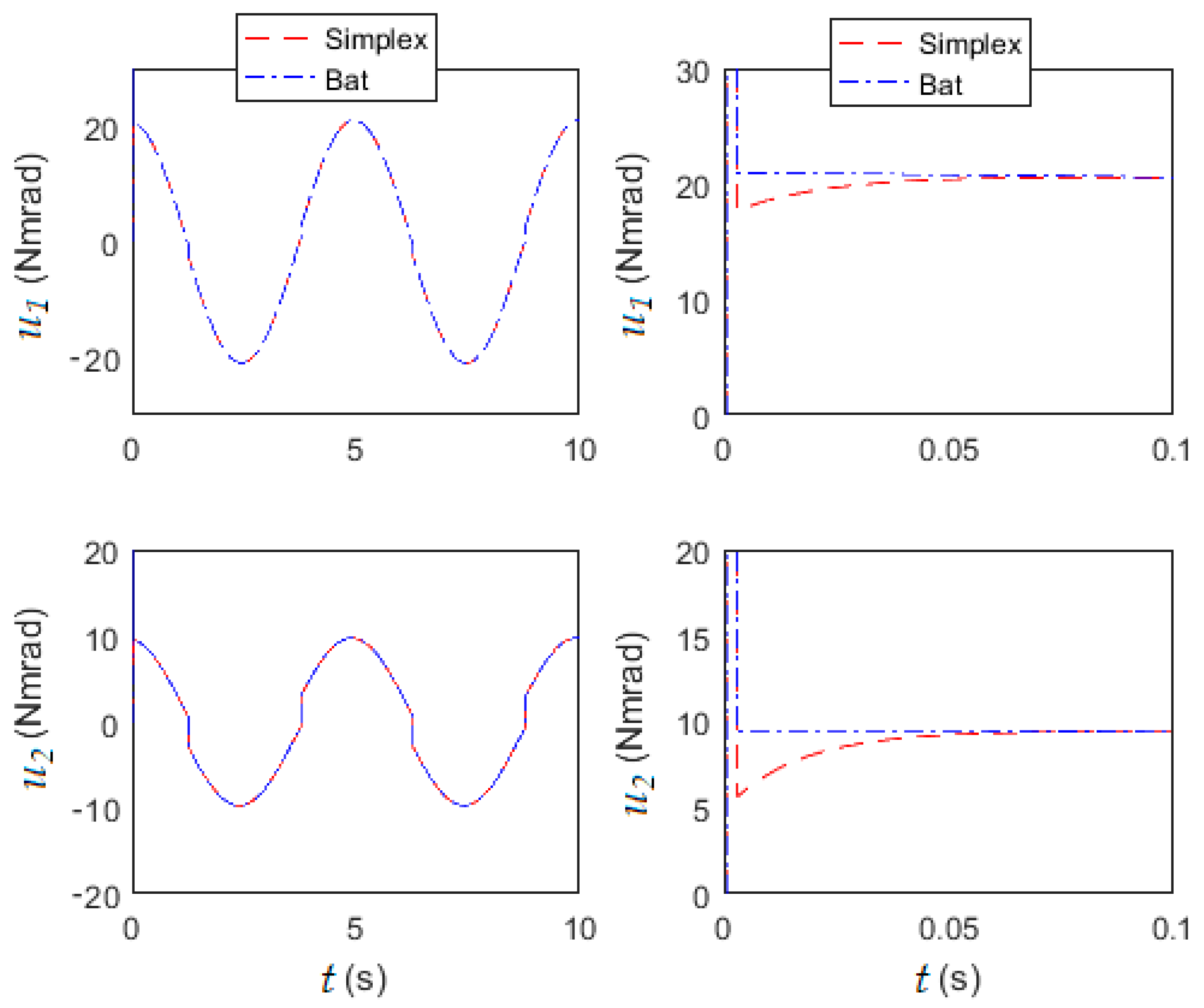
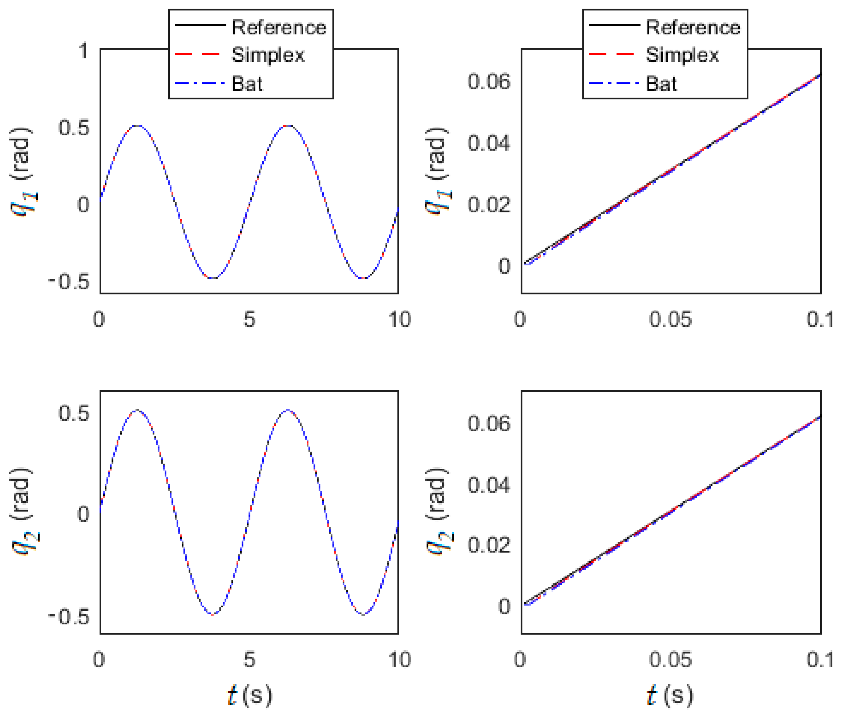
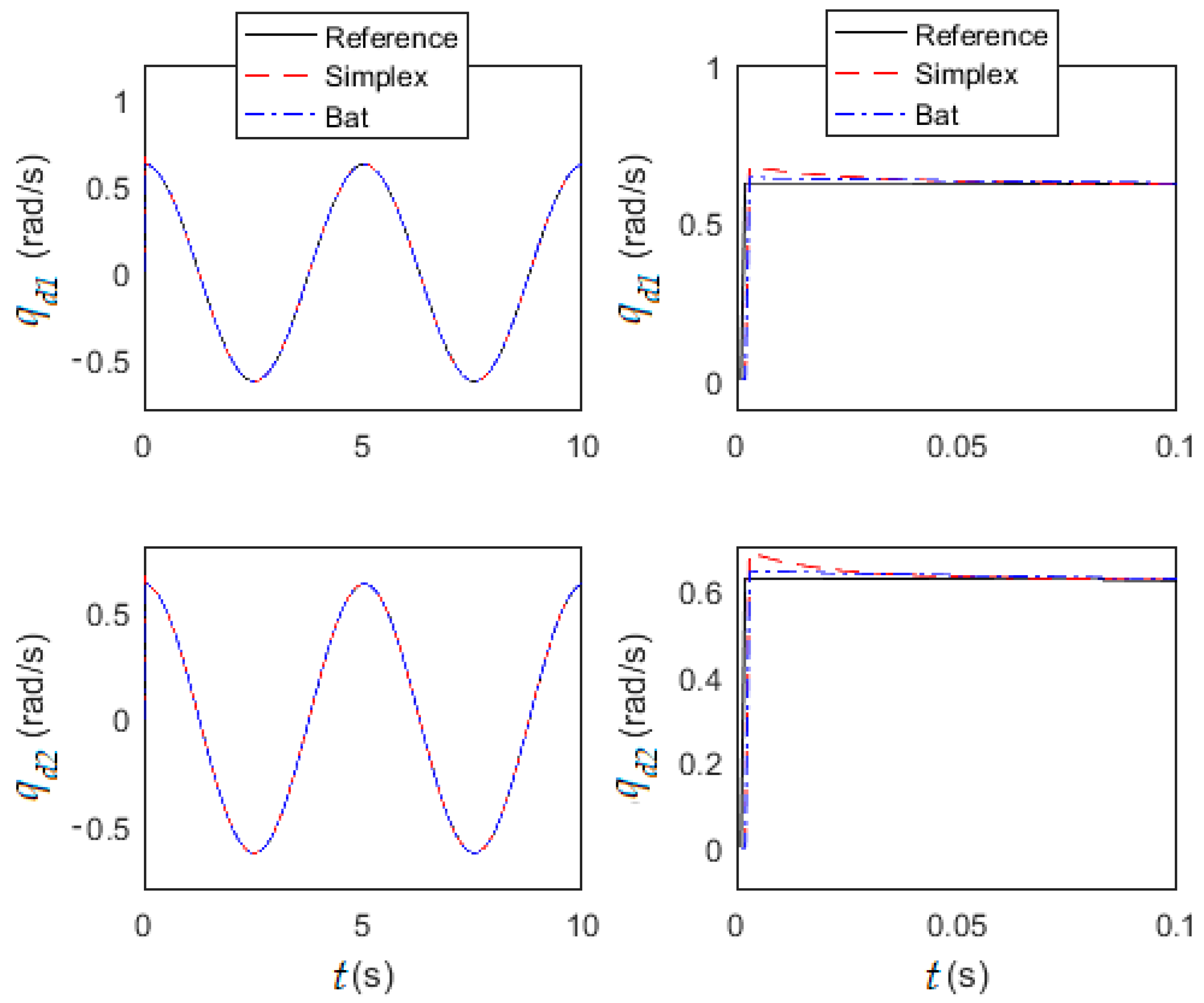
5. Simulations
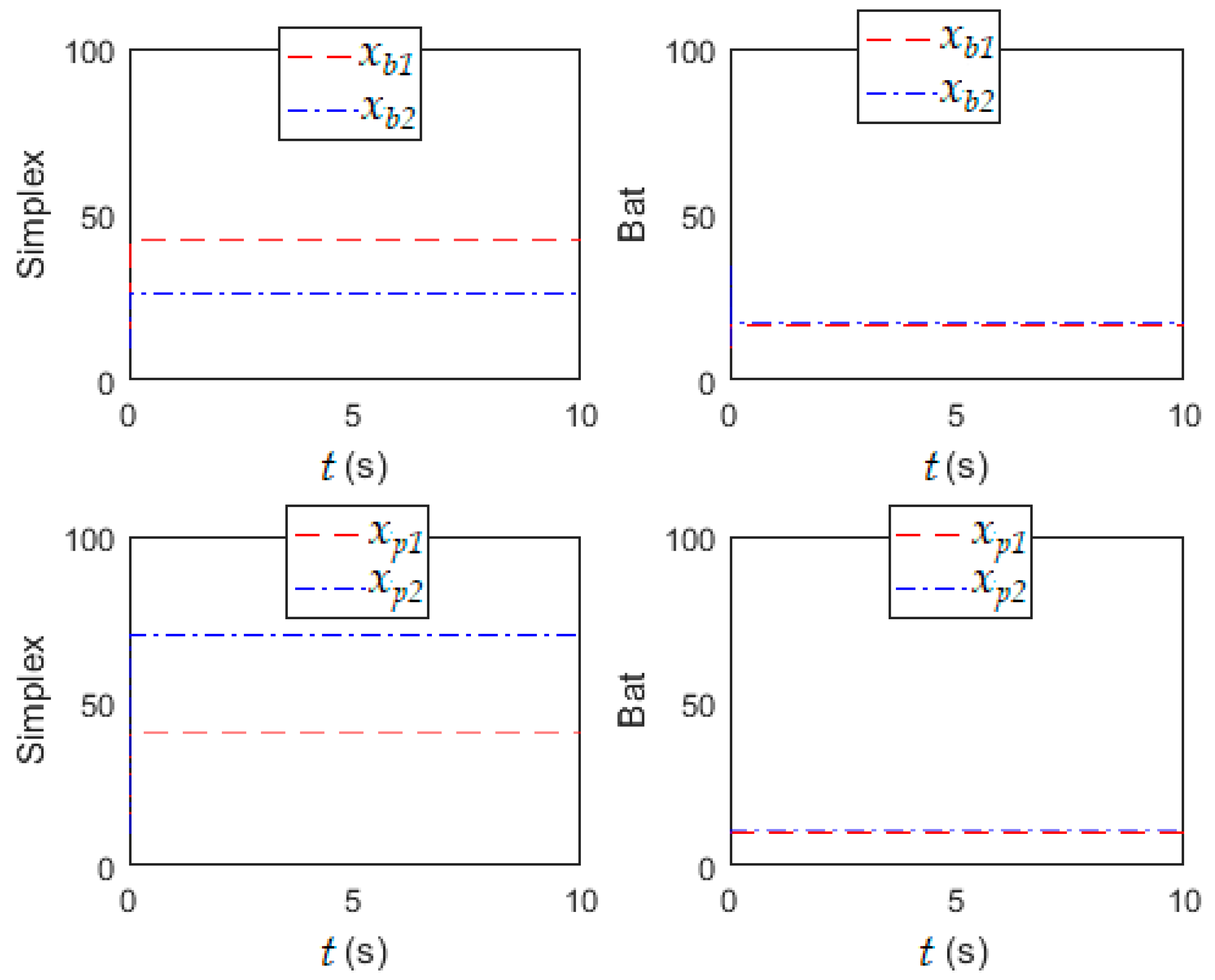
5.1. Optimization of a Sliding Mode Controller for a Two-DOF SCARA Robot Using the Simplex Algorithm
5.2. Optimization of a Sliding Mode Controller for a Two-DOF SCARA Robot Using the Bat Algorithm
6. Discussion
7. Conclusions
Author Contributions
Funding
Institutional Review Board Statement
Informed Consent Statement
Data Availability Statement
Acknowledgments
Conflicts of Interest
References
- Benbouhenni, H.; Bizon, N. Improved Rotor Flux and Torque Control Based on the Third-Order Sliding Mode Scheme Applied to the Asynchronous Generator for the Single-RotorWind Turbine. Mathematics 2021, 9, 2297. [Google Scholar] [CrossRef]
- Solodusha, S.; Bulatov, M. Integral Equations Related to Volterra Series and Inverse Problems: Elements of Theory and Applications in Heat Power Engineering. Mathematics 2021, 9, 1905. [Google Scholar] [CrossRef]
- Le, T.D.; Kang, H.-J.; Suh, Y.-S. Chattering-Free Neuro-Sliding Mode Control of 2-DOF Planar Parallel Manipulators. Int. J. Adv. Robot. Syst. 2013, 10, 22. [Google Scholar] [CrossRef]
- Dal, M.; Teodorescu, R. Sliding Mode Controller Gain Adaptation and Chattering Reduction Techniques for DSP-Based PM DC Motor Drives. Turk. J. Electr. Eng. Comput. Sci. 2011, 19, 532–549. [Google Scholar]
- Swathi, K.; Kumar, G.V.N. Design of intelligent controller for reduction of chattering phenomenon in robotic arm: A rapid prototyping. Comput. Electr. Eng. 2019, 74, 483–497. [Google Scholar] [CrossRef]
- Ferrara, A.; Incremona, G.P.; Sangiovanni, B. Tracking control via switched Integral Sliding Mode with application to robot manipulators. Control. Eng. Pr. 2019, 90, 257–266. [Google Scholar] [CrossRef] [Green Version]
- Kali, Y.; Saad, M.; Benjelloun, K.; Khairallah, C. Super-twisting algorithm with time delay estimation for uncertain robot manipulators. Nonlinear Dyn. 2018, 93, 557–569. [Google Scholar] [CrossRef]
- Jing, C.; Xu, H.; Niu, X. Adaptive sliding mode disturbance rejection control with prescribed performance for robotic manipulators. ISA Trans. 2019, 91, 41–51. [Google Scholar] [CrossRef]
- Vijay, M.; Jena, D. PSO based neuro fuzzy sliding mode control for a robot manipulator. J. Electr. Syst. Inf. Technol. 2017, 4, 243–256. [Google Scholar] [CrossRef] [Green Version]
- Cibiraj, N.; Varatharajan, M. Chattering reduction in sliding mode control of quadcopters using neural networks. Energy Procedia 2017, 117, 885–892. [Google Scholar] [CrossRef]
- Ba, D.X.; Bae, J. A Precise Neural-Disturbance Learning Controller of Constrained Robotic Manipulators. IEEE Access 2021, 9, 50381–50390. [Google Scholar]
- Mobayen, S.; Mofid, O.; Din, S.U.; Bartoszewicz, A. Finite-Time Tracking Controller Design of Perturbed Robotic Manipulator Based on Adaptive Second-Order Sliding Mode Control Method. IEEE Access 2021, 9, 71159–71169. [Google Scholar] [CrossRef]
- Song, T.; Fang, L.; Wang, H. Model-free finite-time terminal sliding mode control with a novel adaptive sliding mode observer of uncertain robot systems. Asian J. Control 2021, in press. [Google Scholar] [CrossRef]
- Xu, Z.; Huang, W.; Li, Z.; Hu, L.; Lu, P. Nonlinear Nonsingular Fast Terminal Sliding Mode Control Using Deep Deterministic Policy Gradient. Appl. Sci. 2021, 11, 4685. [Google Scholar] [CrossRef]
- González-García, J.; Narcizo-Nuci, N.; García-Valdovinos, L.; Salgado-Jiménez, T.; Gómez-Espinosa, A.; Cuan-Urquizo, E.; Cabello, J. Model-Free High Order Sliding Mode Control with Finite-Time Tracking for Unmanned Underwater Vehicles. Appl. Sci. 2021, 11, 1836. [Google Scholar] [CrossRef]
- Yang, X.-S. A New Metaheuristic Bat-Inspired Algorithm. In Nature Inspired Cooperative Strategies for Optimization (NICSO 2010); Springer: Berlin/Heidelberg, Germany, 2010; pp. 65–74. [Google Scholar]
- Yang, X.-S.; He, X. Bat algorithm: Literature review and applications. Int. J. Bio-Inspired Comput. 2013, 5, 141–149. [Google Scholar] [CrossRef] [Green Version]
- Chen, S.-Y.; Yang, B.-C.; Pu, T.-A.; Chang, C.-H.; Lin, R.-C. Active Current Sharing of a Parallel DC-DC Converters System Using Bat Algorithm Optimized Two-DOF PID Control. IEEE Access 2019, 7, 84757–84769. [Google Scholar] [CrossRef]
- Haji, V.H.; Monje, C.A. Fractional-order PID control of a MIMO distillation column process using improved bat algorithm. Soft Comput. 2018, 23, 8887–8906. [Google Scholar] [CrossRef]
- Huang, H.-C. Fusion of Modified Bat Algorithm Soft Computing and Dynamic Model Hard Computing to Online Self-Adaptive Fuzzy Control of Autonomous Mobile Robots. IEEE Trans. Ind. Inform. 2016, 12, 972–979. [Google Scholar] [CrossRef]
- Maroufi, O.; Choucha, A.; Chaib, L. Hybrid fractional fuzzy PID design for MPPT-pitch control of wind turbine-based bat algorithm. Electr. Eng. 2020, 102, 2149–2160. [Google Scholar] [CrossRef]
- Pan, Z.; Quynh, N.V.; Ali, Z.; Dadfar, S.; Kashiwagi, T. Enhancement of maximum power point tracking technique based on PV-Battery system using hybrid BAT algorithm and fuzzy controller. J. Clean. Prod. 2020, 274, 123719. [Google Scholar] [CrossRef]
- Premkumar, K.; Manikandan, B. Bat algorithm optimized fuzzy PD based speed controller for brushless direct current motor. Eng. Sci. Technol. Int. J. 2016, 19, 818–840. [Google Scholar] [CrossRef] [Green Version]
- Rahmani, M.; Ghanbari, A.; Ettefagh, M.M. Robust adaptive control of a bio-inspired robot manipulator using bat algorithm. Expert Syst. Appl. 2016, 56, 164–176. [Google Scholar] [CrossRef]
- Rahmani, M.; Komijani, H.; Ghanbari, A.; Ettefagh, M.M. Optimal novel super-twisting PID sliding mode control of a MEMS gyroscope based on multi-objective bat algorithm. Microsyst. Technol. 2018, 24, 2835–2846. [Google Scholar] [CrossRef]
- Soto, R.; Crawford, B.; Olivares, R.; Niklander, S.; Johnson, F.; Paredes, F.; Olguín, E. Online control of enumeration strategies via bat algorithm and black hole optimization. Nat. Comput. 2017, 16, 241–257. [Google Scholar] [CrossRef]
- Talbi, N. Design of Fuzzy Controller rule base using Bat Algorithm. Energy Procedia 2019, 162, 241–250. [Google Scholar] [CrossRef]
- Rossomando, F.G.; Soria, C.M. Adaptive Neural Sliding Mode Control in Discrete Time for a SCARA robot arm. IEEE Lat. Am. Trans. 2016, 14, 2556–2564. [Google Scholar] [CrossRef]
- Kelly, R.; Santibáñez, V.; Loría, A. Control of Robot Manipulators in Joint Space. In Advanced Textbooks in Control and Signal Processing; Springer: London, UK, 2005; ISBN 978-1-85233-994-4. [Google Scholar]
- Hung, J.Y.; Gao, W.; Hung, J.C. Variable structure control: A survey. IEEE Trans. Ind. Electron. 1993, 40, 2–22. [Google Scholar] [CrossRef] [Green Version]
- Arciuolo, T.F.; Faezipour, M. PID++: A Computationally Lightweight Humanoid Motion Control Algorithm. Sensors 2021, 21, 456. [Google Scholar] [CrossRef]
- Li, Y.; Wang, D.; Zhou, S.; Wang, X. Intelligent Parameter Identification for Robot Servo Controller Based on Improved Integration Method. Sensors 2021, 21, 4177. [Google Scholar] [CrossRef]
- Martinez, D.I.; De Rubio, J.J.; Vargas, T.M.; Garcia, V.; Ochoa, G.; Balcazar, R.; Cruz, D.R.; Aguilar, A.; Novoa, J.F.; Aguilar-Ibanez, C. Stabilization of Robots with a Regulator Containing the Sigmoid Mapping. IEEE Access 2020, 8, 89479–89488. [Google Scholar] [CrossRef]
- Martinez, D.; Rubio, J.; Garcia, V.; Vargas, T.; Islas, M.; Pacheco, J.; Gutierrez, G.; Meda-Campaña, J.; Mujica-Vargas, D.; Aguilar-Ibañez, C. Transformed Structural Properties Method to Determine the Controllability and Observability of Robots. Appl. Sci. 2021, 11, 3082. [Google Scholar] [CrossRef]
- Berardi, M.; D’Abbicco, M.A. Critical Case for the Spiral Stability for 2x2 Discontinuous Systems and an Application to Recursive Neural Networks. Mediter. J. Math. 2016, 13, 4829–4844. [Google Scholar] [CrossRef]
- Difonzo, F.V. A note on attractivity for the intersection of two discontinuity manifolds. Opusc. Math. 2020, 40, 685–702. [Google Scholar] [CrossRef]
- Lee, Y.; Resiga, A.; Yi, S.; Wern, C. The Optimization of Machining Parameters for Milling Operations by Using the Nelder–Mead Simplex Method. J. Manuf. Mater. Process. 2020, 4, 66. [Google Scholar] [CrossRef]
- Visuthirattanamanee, R.; Sinapiromsaran, K.; Boonperm, A.-A. Self-Regulating Artificial-Free Linear Programming Solver Using a Jump and Simplex Method. Mathematics 2020, 8, 356. [Google Scholar] [CrossRef] [Green Version]
- Angeles, J.; Caro, S.; Khan, W.; Morozov, A. Kinetostatic Design of an Innovative Schönflies-Motion Generator. Proc. Inst. Mech. Eng. Part C J. Mech. Eng. Sci. 2006, 220, 935–943. [Google Scholar] [CrossRef] [Green Version]
- Di Gregorio, R.; Cattai, M.; Simas, H. Performance-Based Design of the CRS-RRC Schoenflies-Motion Generator. Robotics 2018, 7, 55. [Google Scholar] [CrossRef] [Green Version]


| Parameter | Symbol | Value |
|---|---|---|
| Minimum gain value | 0 | |
| Maximum gain value | 100 | |
| Minimum gain value | 0 | |
| Maximum gain value | 100 |
| Parameter | Symbol | Value |
|---|---|---|
| Loudness | 0.9 | |
| Pulse rate | 0.9 | |
| Minimum frequency | 0.0 | |
| Maximum frequency | 100 | |
| Minimum gain value | 0 | |
| Maximum gain value | 100 | |
| Minimum gain value | 0 | |
| Maximum gain value | 100 |
| RMSEu1 | RMSEu2 | RMSEe1 | RMSEe2 | |
|---|---|---|---|---|
| Simplex | 214.2696 | 85.3328 | 2.1358 × 10⁻⁵ | 2.1445 × 10⁻⁵ |
| Bat | 203.8097 | 78.6126 | 2.0201 × 10⁻⁵ | 2.0223 × 10⁻⁵ |
Publisher’s Note: MDPI stays neutral with regard to jurisdictional claims in published maps and institutional affiliations. |
© 2021 by the authors. Licensee MDPI, Basel, Switzerland. This article is an open access article distributed under the terms and conditions of the Creative Commons Attribution (CC BY) license (https://creativecommons.org/licenses/by/4.0/).
Share and Cite
Soriano, L.A.; Rubio, J.d.J.; Orozco, E.; Cordova, D.A.; Ochoa, G.; Balcazar, R.; Cruz, D.R.; Meda-Campaña, J.A.; Zacarias, A.; Gutierrez, G.J. Optimization of Sliding Mode Control to Save Energy in a SCARA Robot. Mathematics 2021, 9, 3160. https://0-doi-org.brum.beds.ac.uk/10.3390/math9243160
Soriano LA, Rubio JdJ, Orozco E, Cordova DA, Ochoa G, Balcazar R, Cruz DR, Meda-Campaña JA, Zacarias A, Gutierrez GJ. Optimization of Sliding Mode Control to Save Energy in a SCARA Robot. Mathematics. 2021; 9(24):3160. https://0-doi-org.brum.beds.ac.uk/10.3390/math9243160
Chicago/Turabian StyleSoriano, Luis Arturo, José de Jesús Rubio, Eduardo Orozco, Daniel Andres Cordova, Genaro Ochoa, Ricardo Balcazar, David Ricardo Cruz, Jesus Alberto Meda-Campaña, Alejandro Zacarias, and Guadalupe Juliana Gutierrez. 2021. "Optimization of Sliding Mode Control to Save Energy in a SCARA Robot" Mathematics 9, no. 24: 3160. https://0-doi-org.brum.beds.ac.uk/10.3390/math9243160