Pipeline Two-Phase Flow Pressure Drop Algorithm for Multiple Inclinations

Abstract

A Generalized Additive Model (GAM) is proposed to predict the pressure drop in a gas–liquid two-phase flow at horizontal, vertical, and inclined pipes based on 21 different dimensionless numbers. It is fitted from 4605 points, considering a fluid pattern classification as Annular, Bubbly, Intermittent, and Segregated. The GAM non-parametric method reached high prediction capacity and allowed a great degree of interpretability (i.e., it helped to visualize and test statistical inference), considering that each predictor’s marginal effects could be described, unlike in other Machine Learning (ML) methods. The prediction capacity of the GAM model for the pressure gradient obtained an adjusted $R^2$ and a mean relative error of 99.1% and 12.93%, respectively. This capacity is maintained even when ignoring Bubbly flow in the training sample. A regularization technique to filter some variables was used, but most of the predictors must maintain the model’s high predictive ability. For example, dimensionless numbers such as the Reynolds, Froude, and Weber numbers show p-values of less than 0.01% to explain the pressure gradient in the different flow patterns. The model performs adequately on 500 randomly sampled data points not used to fit the model with an error lower than 15%. The variable importance for the model and the relationship with the pressure gradient is evaluated based on the obtained splines and p-values.

1. Introduction

Transporting fluids in the Oil and Gas Industry, for instance, from the well to the processing plant (upstream sector), represents a challenge. This challenge requires a complex configuration of pipes that contain multiphase mixtures of gases and liquids at different inclinations and operating conditions. The design of this two-phase configuration includes essential parameters for operators such as pressure gradient or void fraction, which are avoided in single-phase flows, in which reliable methods to calculate frictional pressure drop are available (e.g., the Moody chart or Colebrook-White equation). For two-phase flow, there are complex dynamics between the gas and liquid within the pipe that makes these predictions much more challenging [1].

Several approaches estimate or predict the frictional pressure drop in two-phase flows based on empirical correlations such as the ones proposed by Hagedorn and Brown [2] or Beggs and Brill [3]. These correlations depend strongly on the data used and the conditions under which they were built; therefore, their application range is restricted. For example, Hagedorn and Brown’s [2] original correlations’ were not based on conservation and momentum balances, although the development of the original paper’s correlation followed some physical phenomena present in the system. The mechanistic modeling approaches for different pipe configurations were developed later using mass and momentum balances. Overall, most of these models depend on how flow patterns are classified, allowing assumptions about the geometry of the cross-sectional area distribution of the phases, which are necessary to study their interfacial properties. For instance, Xiao, Shonham, and Brill [4] proposed a pressure drop model for Annular, Bubbly, Intermittent, and Stratified flow patterns using the continuity and momentum equations by assuming uniform liquid height in the film zone, which they stated is good enough for most practical applications.

Despite these efforts, mechanistic models such as those by Hasan and Kabir, and Ansari, among others still need to select from various closure laws to work them properly given to their limitations to apply different two-phase flow correlations [5]. Mechanistic models cannot explain some phenomena, so some empirical correlations need to be introduced, and since these closure laws are empirically based, they undermine the objective of mechanistic modeling [5]. An alternative approach uses drift flux models [6], which consider the mixture as a whole rather than two separated phases [7]. In this direction, drift flux models follow a more rigorous approximation than the two-phase mechanistic models; however, they assume homogeneous flow, which can be a strong assumption when the difference of density between fluids is significantly enough like in the case of oil-water systems [8]. Moreover, there are different available empirical flow pattern transition maps based on the phases’ superficial velocities (e.g., Taitel and Dukler [9]), which depend on the flow being near horizontal or vertical. These maps help visualize the most likely flow pattern of the mixture and are essential for any mechanistic model that aims to describe the two-phase flow dynamics. These maps have been improved considering that statistical and machine learning tools such as Neural Networks (NN) and kernels have been considered from a probabilistic-based approach. Overall, Machine Learning (ML) implements data with statistical learning methods and algorithms to “learn” based on some predefined labeled (supervised) or unlabeled (unsupervised) features. Within the supervised approaches they are classification or regression models, whereas in the case of unsupervised learning algorithms for clustering or dimensionality reduction. In this regard, data recollection plays a relevant role to develop these kind of approaches as in work done in the Tulsa Unified Fluid Flow Project (TUFFP) by Zhang et al. [10]. For instance, Amaya-Gómez et al. [11] dealt with the flow pattern classification problem using k-nearest neighbors and a Bayesian approach based on a relevant experimental database. There are other examples that have implemented Machine Learning approaches for two-phase or multiphase related to pattern flow recognition, flow dynamics, liquid hold-up calculation, including Refs. [5,12,13,14,15].

Hybrid approaches combining a probabilistic or a machine learning method with a mechanistic model can help to obtain better estimations of both void fraction and pressure gradient. For example, the probabilistic method proposed by Amaya-Gómez et al. [11] can be implemented jointly with the TUFFP model [10]. The flow pattern classification could be handled with the probabilistic approach, while the momentum and continuity equations would be employed to calculate the pressure gradient. Other alternatives include predicting the flow patterns and pressure gradients based on linear regression or probabilistic methods. For example, Kanin et al. [5] used Random Forest, Gradient Boosting Decision Trees, Support Vector Machines, and Artificial Neural Networks to predict flow patterns, void fraction, and pressure gradients in a three-stage model. Compared to the mechanistic models proposed by Ansari et al. [16], Xiao, Shonham, and Brill [4], and the TUFFP Unified [10,17], the results reported lower prediction errors. Another interesting example is reported by Hernández et al. [18], where the authors use decision trees to identify which phenomenologically based correlations are best to predict in specific flow patterns. The approach of Hernández et al. [18], which selects closure relationships or even different ML models, can also be improved by optimization tools; for example, Mohammadi, Papa, Pereyra, and Sarica [19] show that using a genetic algorithm can improve a mechanistic model 277% by selecting closure relationships.

Although these statistical and machine learning methods may have good predictions, they also lack in-depth interpretability, considering that most of these methods follow a black-box approach that may not provide deep insights into the available data. Consequently, this study seeks to predict the total pressure drop in gas–liquid two-phase flow using statistical methods that facilitate the results’ interpretation. Here, the interpretation is associated with the possibility of evaluating p-value tests, displaying predictors contributions, and estimating predictors’ confidence intervals. These features allow identifying the risk built in the model. For example, confidence intervals can be used to see where the splines effects are dubious because of the lack of observations. Furthermore, p-values can tell which predictors are statistically insignificant and should not be considered. Following these requirements, Generalized Additive Models and Regression Splines would be considered. This strategy retains interpretability and statistical inference capability while having a functional prediction capacity when it is continuous and smooth [20]. Generalized Additive Models (GAM) are a middle ground tool for prediction and can be used to generalize general linear models. GAMs are a tool for both prediction and statistical inference based on a standard generalized model with a link function consisting of a mix of linear or parametric functions of the covariates and other non-parametric non-linear functions. They have been implemented in different fields such as agriculture and medicine. See Hastie and Tibshirani [21] for some applications. Overall, a GAM can be used in any case where linear or logistic regression fits the objective’s scope. GAM can find non-linear relationships between predictors and the response in both the classification and regression settings in addition to the statistical background of linear or logistic methods. The predictors correspond with different well-known dimensionless numbers and the response with the pressure gradient for this work.

Previous Uses of Dimensionles Numbers

In multiphase flow literature, numerous cases implemented dimensionless numbers as inputs for correlation or mechanistic models. Their use is attractive because available databases usually have a limited range of reported substances. Hence, considering correlations based on known dimensionless quantities allows the model to be expanded for different substances if there are sufficient records of the corresponding dimensionless number. One of the most famous models in the two-phase flow, where dimensionless numbers are contemplated, is the Taitel and Dukler [9] mechanistic model for near horizontal inclinations. They manipulate the momentum and mass balance equations mathematically to express them on known dimensionless quantities known as the Lockhart–Martinelli parameter and a dimensionless hydrostatic pressure drop for stratified flow. The correlation works by solving the equations that depend on these dimensionless numbers to obtain the liquid film height, which is then used with geometrical assumptions to find the rest of the interest variables.

The use of dimensionless numbers in mechanistic models is still prevalent. For example, the Ansari, Sylvester, Shoham, and Brill [16] models used the Lockhart–Martinelli parameter, the two-phase mixture Reynolds number, and the friction factors based on the development’s superficial velocities of their model. The mechanistic model of Petalas and Aziz [22] used the Reynolds number of both the gas and liquid phases based on the hydraulic diameters, the Froude number of the liquid phase, and other dimensionless quantities, considering the relationship with parameters to be found, such as liquid film height or wetted perimeter. The model of Zhang et al. [10] implemented dimensionless numbers, both in determining the unified flow model and supporting closure laws. Namely, the closure laws they used for the liquid entrainment in the gas core are based on the gas Weber, Froude, and both liquid and gas Reynolds. Furthermore, they depend on the dimensionless ratio of the densities and viscosities of the phases.

Recent statistical approaches such as Artificial Neural Networks (ANN) or ensembled decision trees also have considered dimensionless numbers as inputs since they improve predictive ability and generalizability for validation. For example, Ozbayoglu and Ozbayoglu [23] published an ANN model to predict frictional pressure losses and flow patterns based on the superficial Reynolds number of both phases as inputs. Other examples include the machine learning approach proposed by Kanin et al. [5] which implements dimensionless features such as the Reynolds and Froude numbers and additional proposed dimensionless quantities. These features train multiple Machine Learning (ML) algorithms, which they cross-compare and obtain high $R^2$ values in their predictions.

This article is organized as follows: Section 2 presents the theoretical framework of the GAM and how flow patterns are mainly classified. Section 3 describes the implemented database and the main dimensionless numbers used as predictors. Section 4 presents the proposed methodology. Section 5 summarizes the essential findings using the GAM model. Finally, Section 6 shows some concluding remarks.

2. Theoretical Basis

2.1. Generalized Additive Models (GAM)

In the case of regression with a continuous response (normal distribution), the model with k covariates, $j-1$ of them with linear effects and $k-j$ with non-linear forms, has the following general expression:

$$Y={\beta }_0+{\beta }_1{x}_1+\cdots +{\beta }_{j-1}{x}_{j-1}+f_j\left(x_j\right)+\cdots +f_k\left(x_k\right)+ϵ$$

(1)

where functions $f_j\left(x_j\right)$ may describe flexible relations estimated non-parametrically, and $ϵ$ is the model’s error, representing the intrinsic random variability. Generalized Additive Models are no different from generalized linear models (e.g., logistic regression) except for non-parametric parts of the function. However, instead of assuming a linear relationship between predictors and linked response, some smooth function is found that represents well the effect of the non-parametric terms on the variable to be predicted. Please note that additivity implies that each of the independent variables has a functional effect on the response Y, and the addition of the terms composes the joint multivariate function. The resulting model has the advantage of being interpretable in the effects of each covariate. This happens because each function is the central effect of the respective variable on the response. When the function is not additive, the high order interactions hide the interpretation, given that margins cannot separate the multivariate function. Please note that interpretability in this model means that each covariate’s effect on the response may be separated; however, if a margin is non-parametrically estimated, there is no analytical expression of the function in general. Moreover, the estimators are defined pointwise and are easier to describe graphically. Another sense in which interpretability is advantageous is that the model can be used to construct p-values and confidence intervals. These can be used to assess the risk of bias and overfitting in the model. In this sense, the modeler can know which covariates have a high degree of confidence in their estimates and if the pressure gradient can be explained more accurately.

The general function in Equation (1) allows including flexible dependence of the response on the covariates. Some smoothness restrictions must be imposed to control that each marginal function truly reflects the relation’s central tendency and is not too influenced by the random error $ϵ$. This process is called regularization and avoids over-fitting to the data. It does not mean that the resulting estimator is necessarily a smooth function, but that the function’s total variation is controlled. As a result, another advantage is that the model, in general, has better predictive performance if it is used to predict the mean response on data points that are out of the sample used to estimate the model, which is a consequence of the non-linear nature of the relationship with the response. Simultaneously, the additive form imposes a structural restriction on the mean multivariate function that avoids the deterioration of the estimations when the number of variables increases, a characteristic of non-parametric methods usually referred to as the curse of dimensionality.

However, this flexibility comes at the cost of finding how to represent the non-parametric functions in some way and choosing how “smooth” they should be [24]. The problem of representation is generally solved by using a finite number of basis functions for each function $f_j\left(x_j\right)$. The following equation defines the non-parametric term as:

$$f_j\left(x_j\right)=\sum _{b=1}^B{b}_{j_b}\left(x_j\right){\beta }_{j_b}$$

(2)

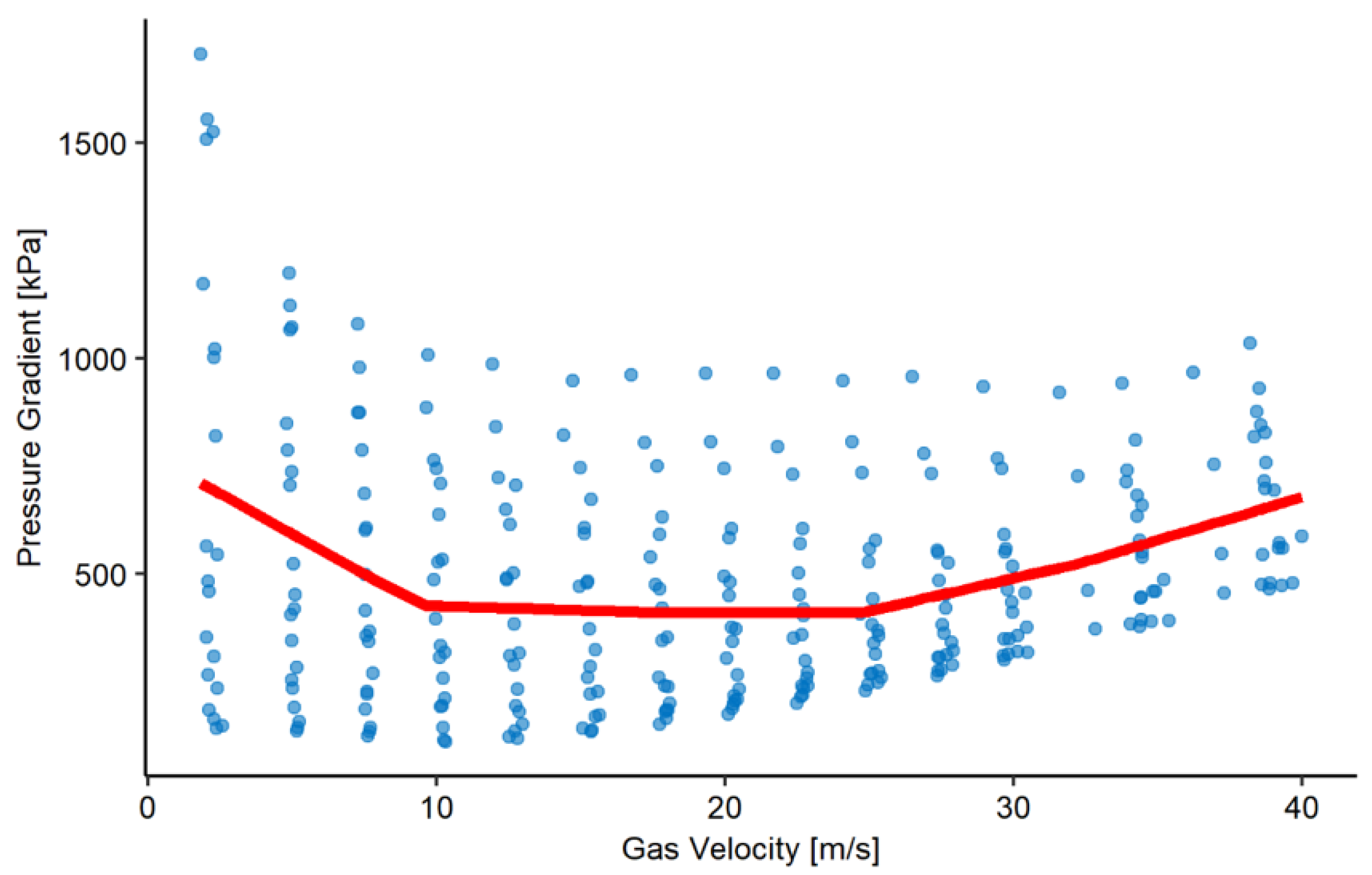
where $b_{j_b}\left(x_j\right)$ is the b-th base function for the covariate $x_j$ and ${\beta }_{j_b}$ are their corresponding coefficients. The most straightforward approach is to use a polynomial basis; nevertheless, this approach has the problem implied by the Taylor theorem, which states that the basis will be a good fit in the neighborhood of a single specified point but not a good representation of the global function. A convenient approach to solve this problem is to use basic functions that are more local, such as a piecewise function defined by a certain number of knots. Figure 1 shows an example of a piecewise linear function with two knots (spline basis with degree 1). A spline basis is a generalization of this idea; in each interval, a polynomial function is defined, requiring that continuity and smoothness are imposed on the knots. With this type of basis, the estimated function’s flexibility may be controlled by the number of knots and each piecewise polynomial degree.

A more convenient alternative for calibrating the GAM, i.e., selecting the appropriate degree of flexibility in each non-parametric function, considers a penalization term on the estimation by ordinary least squares, on which $f_j\left(x_j\right)$ is limited in order to avoid too much variation (wiggliness). A common penalization is the squared second derivative, for which the estimation $({\widehat{\beta }}_0,\cdots ,{\widehat{\beta }}_{j-1},{\widehat{f}}_j,\cdots ,{\widehat{f}}_k)$ results of minimizing:

$$\sum _{i=1}^n{\left(y_i-{\beta }_0-\cdots -{\beta }_{j-1}{x}_{j-1,i}-f_j\left(x_{ji}\right)-f_k\left(x_{ki}\right)\right)}^2+\sum _{h=j}^k{\lambda }_h\int f_h^{″}{\left(x_h\right)}^{2}d{x}_h$$

(3)

where $y_i$ and $x_{ji}$ represents the i-th observation of the response variable and the j-th covariate, respectively. The parameters ${\lambda }_h$ must be calibrated to use the optimal degree of flexibility.

Since the smoothness parameters of the splines are unknown at the start of the algorithm, they are initialized, assuming they do not affect the response. The algorithm cycles find the smoothing parameter (${\lambda }_h$) of each of the non-parametric terms until they reach a stable value. This algorithm is known as backfitting [21]. The convergence of the method is not only fast but guaranteed, with the only restriction that the splines for each covariate $x_j$ are centered [26]:

$$\sum _{i=1}^n{f}_j\left(x_{ji}\right)=0$$

(4)

This condition implies that the splines do not represent the variable’s marginal effects on the response but on the centered response (the mean is subtracted). This situation influences the interpretation of the statistical inference results but not the model’s predictive capability. The primary advantage of GAM models is interpretability and hypothesis testing. For example, the following hypothesis can be considered:

Ho: 

Variable X is in the model.

Ha: 

Variable X is not in the model.

This can be done, as in linear regression, using the F partial test as follows [20]:

$$F={\displaystyle \frac{{\displaystyle \frac{SS{E}_{reduced}-SS{E}_{full}}{d{f}_{reduced}-d{f}_{full}}}}{MS{E}_{full}}}$$

(5)

where SSE and MSE represent the sum and mean of the reduced and the entire model’s square residuals; moreover, df represents the degrees of freedom of each model (the number of parameters used in it). The F statistic can be interpreted as any statistical test. If it has a higher value than a specified significance level in the corresponding accumulated density distribution, then the null hypothesis can be rejected. There can also be a hypothesis made on the nature of the parameter, as shown below:

Ho: 

Variable X has a linear effect.

Ha: 

Variable X has a nonparametric effect.

These tools are a definite advantage that improves the model’s interpretability compared to other machine learning approaches such as Neural Networks or ensembled trees.

2.2. Flow Patterns Considered

Flow pattern classification can be ambiguous, depending on the methodology of each author. For example, Aggour [27] classified patterns between annular (froth and mist), bubble (froth), Slug, Slug Froth, and transitions between slug-bubble and slug-annular. Brito [28] classified them between Annular, Bubble, Intermittent Flow, which combines Slug Flow and Elongated Bubble, and Stratified Wavy. In the database used, each author has their way of naming each flow pattern. Therefore, to have a consistent classification and broader categories, the categories shown in

Table 1. Classification of flow patterns for prediction.

Flow Pattern Considered
	Annular Flow (A)	Bubbly Flow (BF)	Intermittent Flow (IT)	Segregated Flow (SG)
Original description	-Annular	-Bubble	-Intermittent/Annular	-Stratified
	-Annular/Intermittent	-Bubble/Intermittent	-Intermittent/Bubble	-Stratified Wavy
	-Annular Froth	-Bubble Froth	-Slug Churn
	-Annular Mist		-Slug Flow
	-Annular Wavy		-Slug Froth
	-Churn Annular

are considered.

The classification proposed in Table 1 is consistent with previous works in the literature such as those by Amaya-Gómez et al. [11], Brito [28], Fan [29], and Mantilla [30]. Furthermore, transitions between flow patterns can be seen, especially from intermittent to annular and intermittent to bubble. Figure 2 shows the flow patterns used in this document and illustrates their characteristics. It can be seen in Figure 2 that bubbly flow refers to small spherical bubbles of gas, which are dispersed in the liquid phase. Intermittent flow is comprised of large and elongated bubbles of gas that form liquid pistons of considerable length. Stratified flow is a typical flow with a well-defined interface between the fluids is formed for any cross-sectional cut of the pipe. Stratified Flow disappeared for an inclination greater than 70${}^{\circ }$ (upward direction). Annular flow occurs at high void fractions and generally is comprised of a high-velocity gas phase that pushes the liquid phase outwards.

3. Materials: Database and Dimensionless Numbers

3.1. Database Presentation

This work implements the data reported at the TUFFP database, including 43,565 records, out of which 5011 registered both a flow pattern and total pressure drop. There are 4605 cases of pipes inclined upwards and 406 cases of pipes inclined downwards. A negative $\Delta P$ sign implies the pipe gains pressure instead of losing it because of a drop in the potential energy. The database used in the development of the proposed model consists of these 5011 points; these records are described in more detail in

Table 2. Overview of the data of each author in the database. Diameter, L/D ratio, superficial velocities of the phases, angle of inclination, flow patterns, temperature, pressure, and pressure gradient are presented.

Author	Data	D [mm]	$\mathit{L}/\mathit{D}$	${\mathit{V}}_{\mathit{L}}^{\mathit{S}}$ [m/s]	${\mathit{V}}_{\mathit{G}}^{\mathit{S}}$ [m/s]	$\mathit{\theta }$ [${}^{\circ }$]	FP	T [${}^{\circ }$C]	P [kPa]	$\Delta \mathit{P}/\mathit{L}$ [kPa/m]
Aggour [27]	412	11.7	130	0.3139–10.58	0.07–96	90	A, BF, IT	20–39	106–493	0.176–68.52
Alsaadi [25]	288	76.2	232	0.0099–0.101	1.83–40	2 to 30	A, IT, SG	20	100	0.11–1.71
Andritsos [31]	535	25.1–95.3	105–616	0.0003–0.335	0.8–98.9	0	SG	10–27	98–196	0–2.23
Asante [32]	476	25.4–76.2	499–1496	0.0001–0.2	15–30	0	A, SG	15	270	0.001–0.04
Brito [28]	346	50.8	374	0.0097–2.961	0.09–7.7	0	A, BF, IT, SG	21–50	102–211	0.013–7.24
Chung et al. [33]	159	50.8	447	0.0476–0.704	0.28–7.8	−90	A, SG	21–49	109–232	−4.419–0.7
Fan [29]	321	50.8–149.6	335–377	0.0003–0.052	4.93–25.7	−2 to 2	A, IT, SG	15–17	101–222	0.005–0.72
Gockal [34]	183	50.4	375	0.01–1.76	0.09–20.3	0	A, IT, SG	21–38	101	0.033–18.49
Güler-Quadir [35]	102	88.9	8099	0.0366–1.667	0.12–17.7	90	A, BF, IT	20	102	0.45–4.25
Karami [36]	106	152.4	370	0.01–0.027	7.4–22.6	0	SG	22	163	0.011–0.1
Kokal [37]	870	25.8–76.3	313–931	0.03–3.048	0.03–19.4	−9 to 9	IT	11–31	227–365	−1.101–9.62
Kouba [38]	52	76.2	418	0.1524–2.137	0.3–7.4	0	IT	14–42	196–386	0.001–0.03
Mantilla [30]	142	50.8–152.4	53–253	0.0033–0.1	1.5–82.2	0	A, SG	20	104–224	0–6.26
Mora and Zegrí	39	21	228.6	0.0481–1.623	0.22–10.6	0	A, BF, IT, SG	20	103–271	0.006–3.29
Rezkallah [39]	380	11.7	130	0.0219–10.577	0.05–129.6	90	A, BF, IT	19–31	96–403	–0.158–62.7
Skopich [40]	35	50.8–101.6	150–300	0.009–0.05	7.99–29.5	90	A	29–37	104–129	0.176–1.48
Sujumnong [41]	232	11.7	130	0.0457–8.46	0.03–118.4	90	A, BF, IT	17–32	101–343	0.475–62.89
Vijay [42]	333	11.7	130	0.0122–10.607	0.05–140.3	90	A, BF, IT	20–31	99–513	0.276–90.58
Minimum		11.7	53	0.0001	0.03	–90		10	96	−4.419
Maximum		152.4	8099	10.607	140.3	90		50	513	90.58

.

This database comprises 18 references, out of which some of them are commonly used to validate different mechanistic models and correlations experimentally, such as the data of Andritsos [31] being used to validate the model of Zhang et al. [17]. Table 2 shows the maximum and minimum values for the primary measurements of the database, including the diameter, length-to-diameter ($L/D$), superficial velocities ($V_L^S$ and $V_G^S$), the angle of inclination of the pipe ($\theta$), the flow pattern classifications they contain, temperature, pressure, and pressure gradient. From these variables, the last one is to be predicted. Flow patterns are classified in the database as 22.31% annular, 6.41% bubbly, 44.12% Intermittent, and 27.16% segregated.

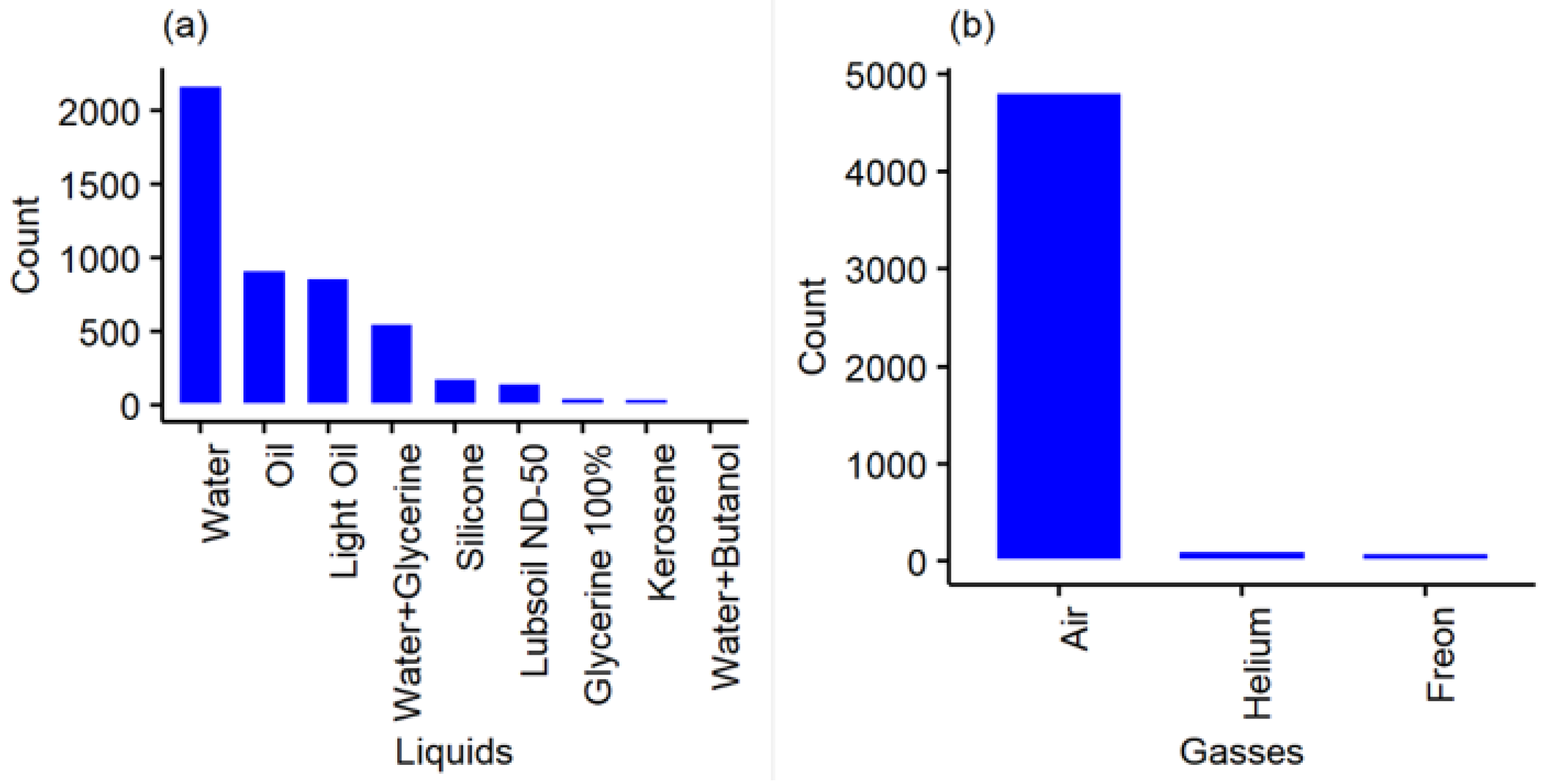
Figure 3 presents the distribution of the liquids and gases used in the database. There are more substances in the liquid phase, but around two thirds of the records used water or glycerin dilutions. The gas phase is composed mainly of air and should not be generalizable for lighter or denser gases. This problem can be solved using dimensionless numbers, as will be described in this work.

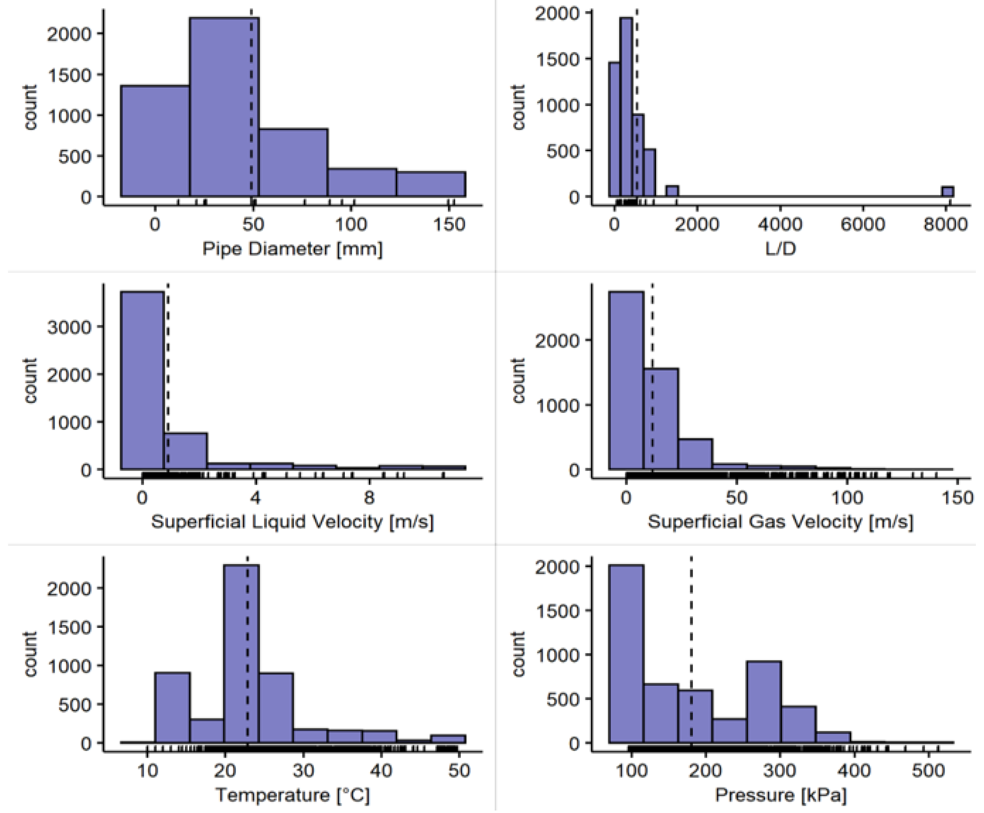
Figure 4 shows the distribution of the pipes’ diameter, L/D relation, superficial velocities, temperature, and pressure of the pipe. It can be seen in Figure 4 that the database cases have temperature readings in conditions near ambient temperature. This is a long, vertically inclined, water-air pipe. Regarding the pressure, most of the records reported near-standard pressure, but there are also pressurized pipes.

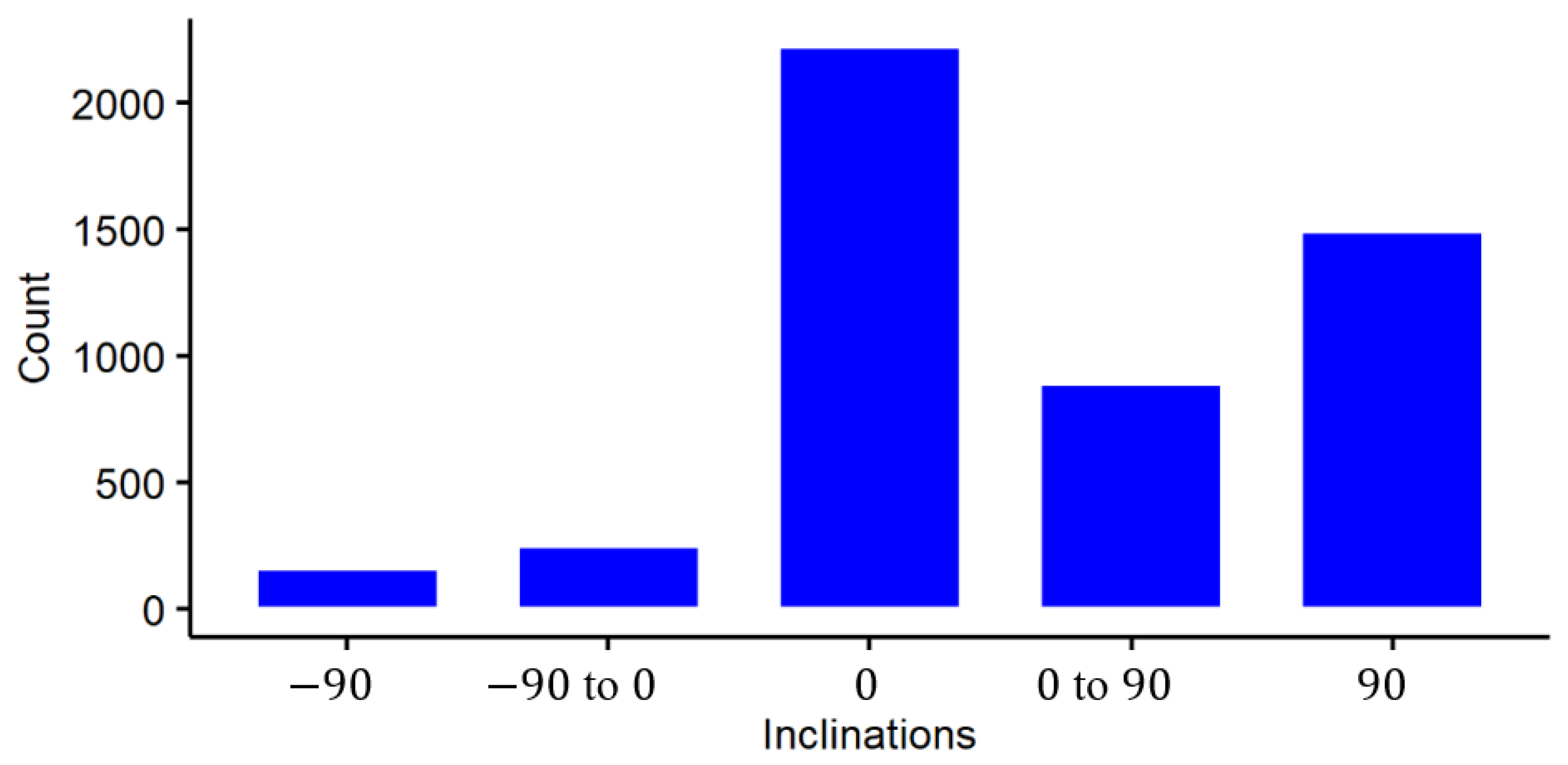
Figure 5 depicts the pipe inclinations, obtaining that 29.81% of the records had vertical upward pipes (i.e., 90${}^{\circ }$) and 3.2% vertical downward pipes (i.e., −90${}^{\circ }$), 44.3% horizontal pipes, and 22.7% inclined pipe cases. More downward cases should be included to improve the database. Figure 5 shows there must be precautions to generalize the final model as a tool for predicting pressure drop in any condition, especially considering the inclination distribution and the overrepresentation of water and air mixtures in the database. However, dimensionless numbers are the chosen strategy to draw broader conclusions from the model proposed in this work.

3.2. Dimensionless Numbers

This work aims to propose a sufficiently robust pressure drop predictive model, seeking to use less training data to be commercially viable. Therefore, it is essential to use known dimensionless numbers as predictors in the database, such as those presented in

Table 3. Dimensionless numbers considered in this work as predictors.

Dimensionless Number	Symbol	Equation	Relationship Explained
Gas Quality	$w_G$	$$\frac{\dot{m_G}}{\dot{m_G}+\dot{m_L}}$$ (6)	Gas mass flow rate to total flow rate
Gas Reynolds	$R{e}_G$	$$\frac{{\rho }_G{V}_G^{S}D}{{\mu }_G}$$ (7)	Inertial forces to viscous forces
Liquid Reynolds	$R{e}_L$	$$\frac{{\rho }_L{V}_L^{S}D}{{\mu }_L}$$ (8)
Mixture Reynolds	$R{e}_M$	$$\frac{{\rho }_M{V}_M^{S}D}{{\mu }_M}$$ (9)
Gas Weber	$W{e}_G$	$$\frac{{\rho }_G{V_G^S}^{2}D}{\sigma }$$ (10)	Inertial forces to surface tension
Liquid Weber	$W{e}_L$	$$\frac{{\rho }_L{V_L^S}^{2}D}{\sigma }$$ (11)
Mixture Weber	$W{e}_M$	$$\frac{{\rho }_M{V_M^S}^{2}D}{\sigma }$$ (12)
Gas Froude	$F{r}_G$	$$\frac{V_G^S}{\sqrt{gD}}$$ (13)	Intertial forces to gravity
Liquid Froude	$F{r}_L$	$$\frac{V_L^S}{\sqrt{gD}}$$ (14)
Mixture Froude	$F{r}_M$	$$\frac{V_M^S}{\sqrt{gD}}$$ (15)
Gas friction factor	$f_G$	$$CR{e}_G^{-n}$$ (16)	Friction factors as in single-phase flow *.
Liquid friction factor	$f_L$	$$CR{e}_L^{-n}$$ (17)
Interfacial friction factor	$f_I$	$$f_G\left(1+14.3\sqrt{1-w_G}\left(\sqrt{\frac{V_G^S{\rho }_G}{{\rho }_{0G}}}\right)\right)$$ (18)	Interfacial friction factor approximation for segregated/ annular flow.
Froude Rate	$F_t$	$${\left(\frac{w_G^3{({\dot{m}}_G+{\dot{m}}_L)}^2}{{\rho }_G^{2}gD(1-w_G)A^2}\right)}^{0.5}$$ (19)	Vapor Kinetic Energy to the energy required to lift the liquid
Y Tailel Dukler Number	$Y_{TD}$	$$\frac{2D(\Delta \rho )gsin\left({\theta }_{rad}\right)}{f_G{\rho }_G{V_G^S}^2}$$ (20)	Hydrostatic pressure loss to gas frictional pressure loss
Eötvös	$E_o$	$$\frac{g{D}^2({\rho }_L-{\rho }_G)}{\sigma }$$ (21)	Gravitational to capillary forces.
Lockhart Martinelli	$\chi$	$$\frac{f_L{\rho }_L{V_L^S}^2}{f_G{\rho }_G{V_G^S}^2}$$ (22)	Frictional liquid loss to Frictional gas loss.
Viscous number	$N_{\mu }$	$$\frac{V_M^S{\mu }_L}{g{D}^2\Delta \rho }$$ (23	Viscous forces to gravitational forces
Length Diameter Ratio	$L/D$	$$\frac{L}{D}$$ (24)	Pipe geometry
Dimensionless Temperature	$\tilde{T}$	$$\frac{T}{T_0}$$ (25)
Dimensionless Pressure	$\tilde{P}$	$$\frac{2P_o}{f_G{\rho }_G{V_G^S}^2}$$ (26)	The initial pressure of pipe to gas pressure loss.

* C is 16, and n is 1 for $R_e$< 3000 (Laminar). C is 0.046, and n is 0.2 for $R_e \ge$ 3000 (Turbulent). As used by Taitel and Dukler.

.

In Table 3, there are present some mixture properties. All of them are defined the same way; for example, mixture density is defined as:

$${\rho }_M=w_G{\rho }_G+(1-w_G){\rho }_L$$

(27)

Every mixture property is defined as in the last equation except mixture velocity because it is traditionally defined in two-phase flow literature as:

$$V_M^S=V_G^S+V_L^S$$

(28)

3.3. Notes on the Dimensionless Numbers Selected

There are multiple ways to define dimensionless numbers; mechanistic models for two-phase flow can also be enriched using geometrical parameters such as the hydraulic diameter or wetted perimeter. Since this work follows a statistical-based model, the dimensionless numbers selected contemplated only those based on easily measured variables. In this regard, geometrical considerations were not considered. Some considerations of the dimensionless shown in Table 3 are described below:

• Gas Quality $w_g$ serves as a proxy for the void fraction of the model. While the void fraction can give more information about the two-phase flow system, it would require a two-step model to be calculated. This two-step model can be contemplated as a future improvement of the proposed model.
• The Reynolds $Re$, Weber $We$, and Froude $Fr$ numbers are defined using superficial velocities and the nominal diameter. Although this is a simple definition for two-phase flow, the statistical model can find non-linear relationships and does not need to have as detailed information as in a mechanistic model. To include both phases’ information, the superficial velocities of the liquid, phase, and mixture are contemplated (Equation (28)). Therefore, three different dimensionless numbers (liquid, gas, and mixture) are based on the velocity used. Multiple mechanistic models and statistical models have used these numbers to calculate two-phase flow dynamics.
• The friction factors of the liquid and gas phases are defined as reported by Taitel and Dukler [9]. The interfacial friction factor expression uses the expression used by Zhang et al. [10], which is a closure law of that mechanistic model.
• The Froude rate $F_t$ has been used in different studies to calculate void fraction. Graham et al. [43] obtained a correlation for the void fraction using the Froude rate and the Lockhart–Martinelli parameter $\chi$ in the stratified flow pattern and nearly horizontal pipes. The idea behind their inclusion is to incorporate further information about the void fraction.
• The Y Taitel–Dukler number was used in Taitel’s and colleagues’ 1976 correlation Taitel and Dukler [9]; they found this grouping was relevant for nearly horizontal gas–liquid flow. The Lockhart–Martinelli parameter also appears as a relevant dimensionless grouping in the same study. The idea to adimensionalize the loss of the hydrostatic pressure based on the gas pressure loss is used in this document when defining the dimensionless pressure $\tilde{P}$.
• The Eötvös number $E_o$ is relevant for small diameter pipes because it captures the system’s capillary forces well. The dominance of the surface tension can help to predict flow pattern maps where superficial tension dominates. Brauner and Moalem [44] found surface tension maps and used the Eötvös number to define where superficial tension dominated as part of their analysis.
• The viscous number $N_{\mu }$ is a dimensionless grouping used by Al-Safran et al. [45] to develop an empirical model that tries to correlate liquid hold-up using different dimensionless groupings for two-phase slug flow.
• The length to diameter ratio and dimensionless temperature are used since there is information available in the database used in this model.

4. Methodology

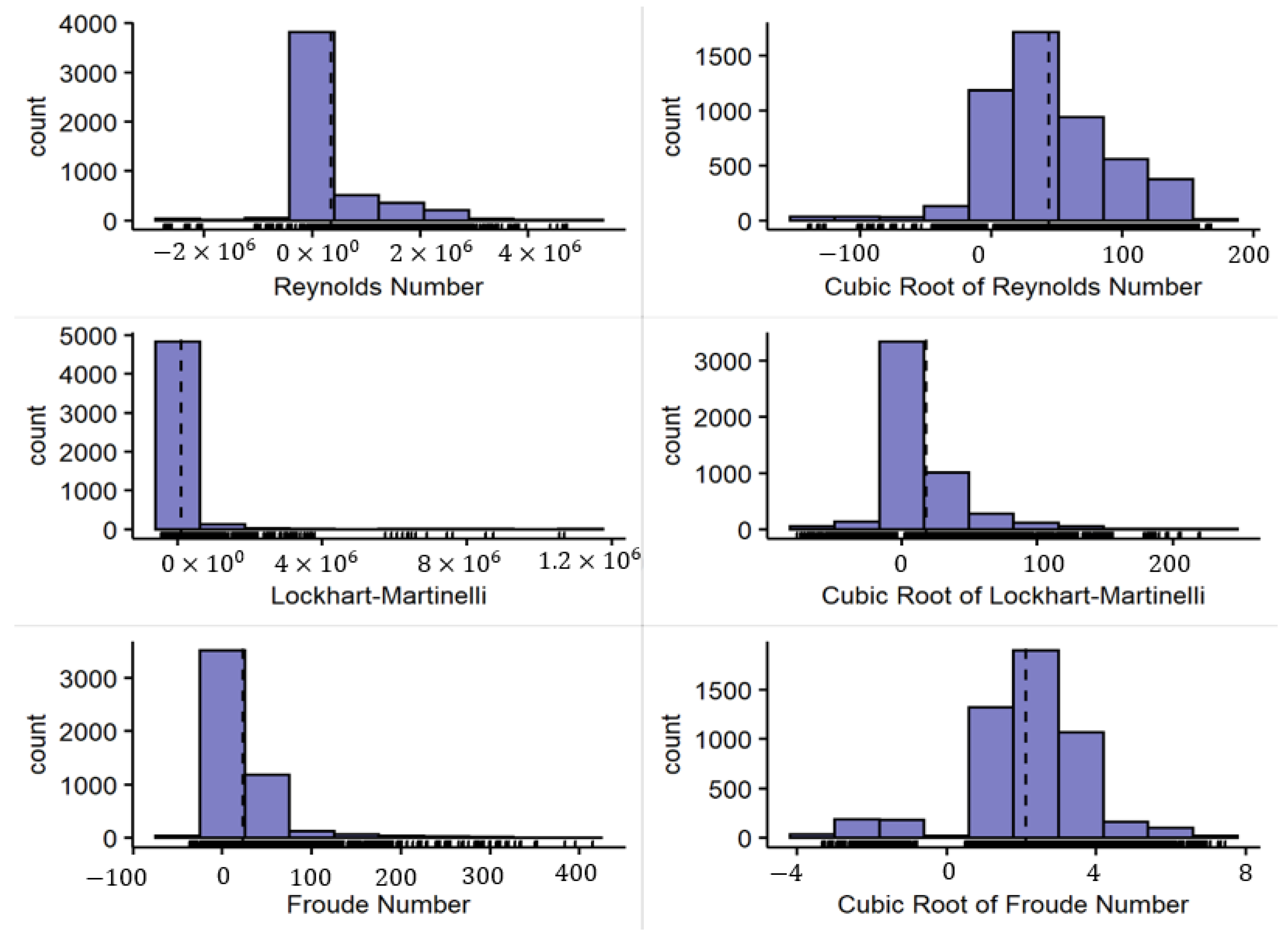
The distribution of the dimensionless numbers throughout the database is smoother than the non-processed parameters. Furthermore, the ranges of applicability of the model can be interpreted in the ranges of the dimensionless numbers, which substantially improves the model’s generalizability. Figure 6 shows the histograms of some of these dimensionless numbers.

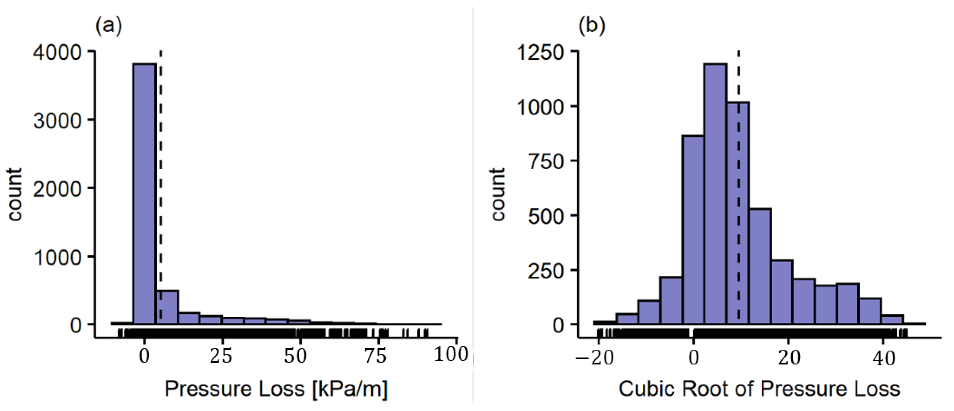
Figure 7a shows the distribution of the response variable (i.e., the pressure gradient). This histogram is left-skewed (e.g., the mean is left to the main peak), so using the correct transformation can improve the normality of the data, which for GAM is not a requirement, but it still can help improve the prediction. The proposed transformation is a cubic root as depicted in Equation (29), which can be used even for negative numbers, unlike a logarithmic transformation. The obtained transformation for the variable response is shown in Figure 7b. Please note that it improves the shape of the histograms. Most of the dimensionless numbers used have similar histogram distributions. As shown in Figure 7b, the cubic root transformation centers the data distribution and reduces skewness. This transformation helps the regression method.

$$Y=\sqrt[3]{{\displaystyle \frac{\Delta P}{L}}}$$

(29)

Additionally, most collinear predictors (i.e., more correlated variables) were removed to reduce the set of predictors from Table 3 using the findCorrelations function in the caret package in R-3.6.3. For this purpose, a correlation threshold of 0.85 high was used to prevent valuable information from being removed from the model. Predictors with a higher correlation than the threshold were the gas Reynolds and the mixture Froude, so they were discarded from the model.

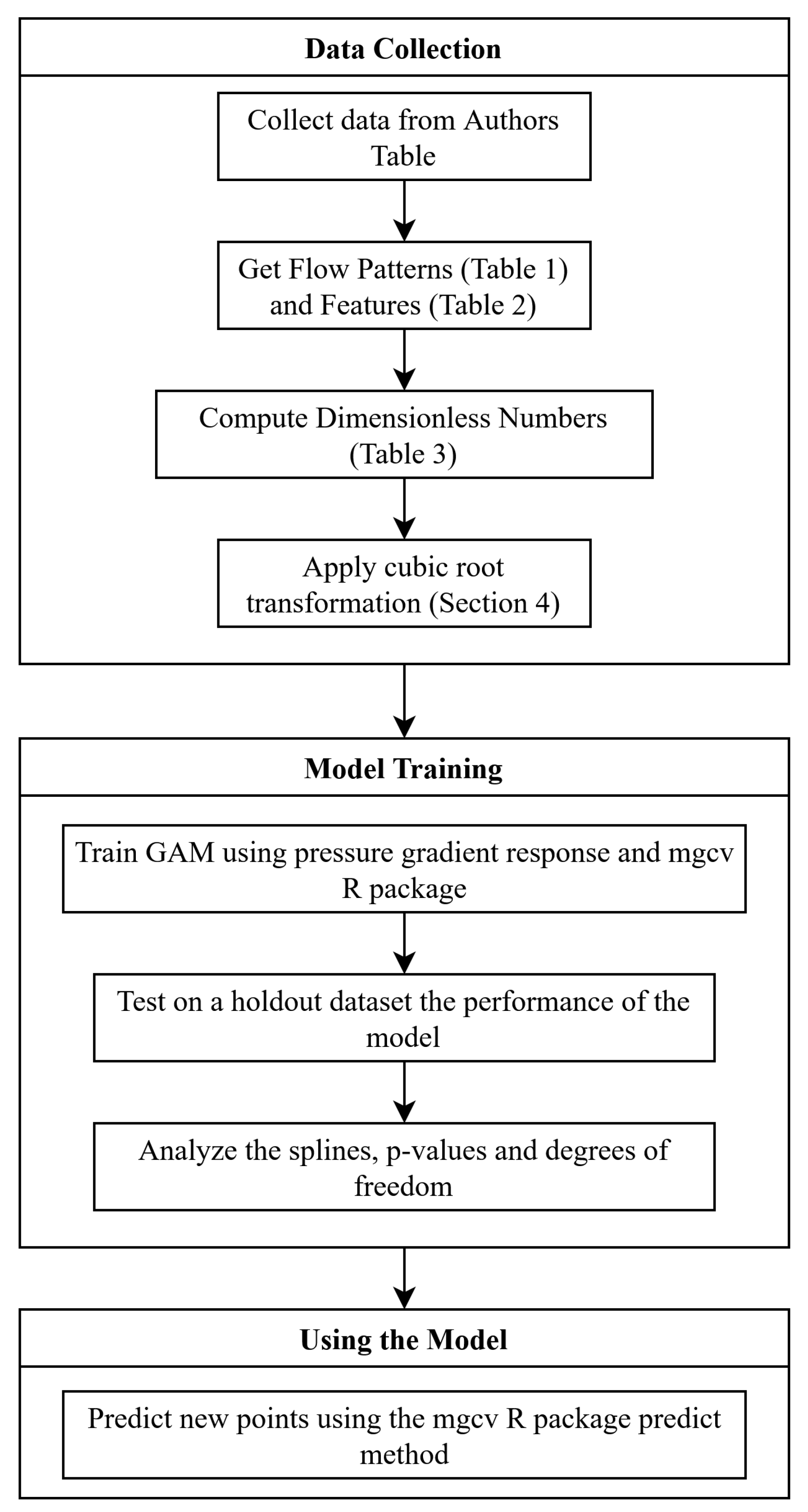
The model assumes that all splines are non-parametric thin-plate splines, yet since these splines are penalized, some of them can end having linear relations with the response. In the final model, to be precise, 19 dimensionless numbers were used, so the model was comprised of 57 non-parametric different covariates since each dimensionless number and flow pattern interaction is considered and since Bubbly flow was merged with the Intermittent flow. The proposed methodology is shown in Figure 8, following a data collection, model training, and using the model to predict the pressure drop.

The GAM was fitted using the mgcv library in R, built by Simon Wood [24]. It has been used in multiple applications in different fields [24]. For each of the covariates with non-linear relation, the basis representations used were thin-plate regression splines that are low-rank smoothers, meaning that they have fewer coefficients than data to smooth. The main idea of this approach is to use a penalized model as the one represented in Equation (3), on which the resulting basis representation is in the form of splines with knots placed on each of the observed points xi. The mgcv library uses different computational approaches to fit the splines in a fast and efficient way. As described in Section 2.1, the calibration of smoothing parameters is performed by generalized cross-validation (GCV). This method is very close to leave-one-out cross-validation (LOOCV), on which the prediction performance is measured on each data point that is left out of the sample. LOOCV fits the model on all the points except one, then evaluates the model performance on that point. Then, LOOCV takes each point in the sample and repeats the procedure, averaging each out-of-sample point’s mean square error. GCV is a less computationally demanding but accurate approximation.

5. Results and Discussion

5.1. Predictive Capability

There are multiple ways to calibrate a GAM; both the predictors and the complexity of each spline must be found in a way the model performs better on a test dataset. Section 1 shows that the splines could be calibrated using the back-fitting algorithm and the thin-plate spline definition. Marra and Wood [46] conducted a study on variable selection. The conclusion was that shrinkage approaches perform significantly better than competing methods in terms of predicting ability. The best-performing methods of variable selection were the double penalty and the eigenvalue shrinkage approaches. Because of the more straightforward interpretability of the double penalty approach, it is considered for this study. In either case, both approaches were the best methods for variable selection, just as compared by Marra and Wood [46].

The double penalty method works using all the predictors from Table 3 except the ones removed due to their high correlations under a regularization method such that fewer essential predictors are taken out of the model. The double penalty method is similar to LASSO (Least Absolute Shrinkage and Selection Operator) variable selection in which the optimization objective function is changed so that models with fewer variables are preferred. It is a double penalty method because both the thin-plate splines and the objective function are penalized. Some splines are taken out of the model, and the ones staying are not too complex.

Figure 9a shows the results obtained by the GAM using all the predictors with the double penalty approach. Figure 9b shows the case where the GAM is calibrated with all the data except for 500 points randomly sampled from the original data set, then validating the results on these points such that the predictive capability of the model is shown for new data. Please note that the model follows closely the mean and is contained in the 15% error lines on downward (negative) and upward (positive) cases.

The relative error (RE) is defined as the absolute difference between the response and predicted values over the original or observed response. The mean relative error (MRE) for each flow pattern will then be used to illustrate the model’s predictive capability (Equation (30)) where $m_j$ is the total number of observations in the corresponding flow pattern.

$$MRE=\sum _{i=1}^{m_j}{\displaystyle \frac{|Y_{obs}^i-Y_{pred}^i|}{m_j{Y}_{obs}^i}},\forall j\in \{A,BF,IT,SG\}$$

(30)

Furthermore, for model comparison, AIC, or the Akaike information criterion based on the model’s likelihood function, was considered. The measure tries quantifying a trade-off between goodness of fit and the number of parameters in the model, penalizing overfitting. Then the AIC can be compared between models, where a smaller value means better quality.

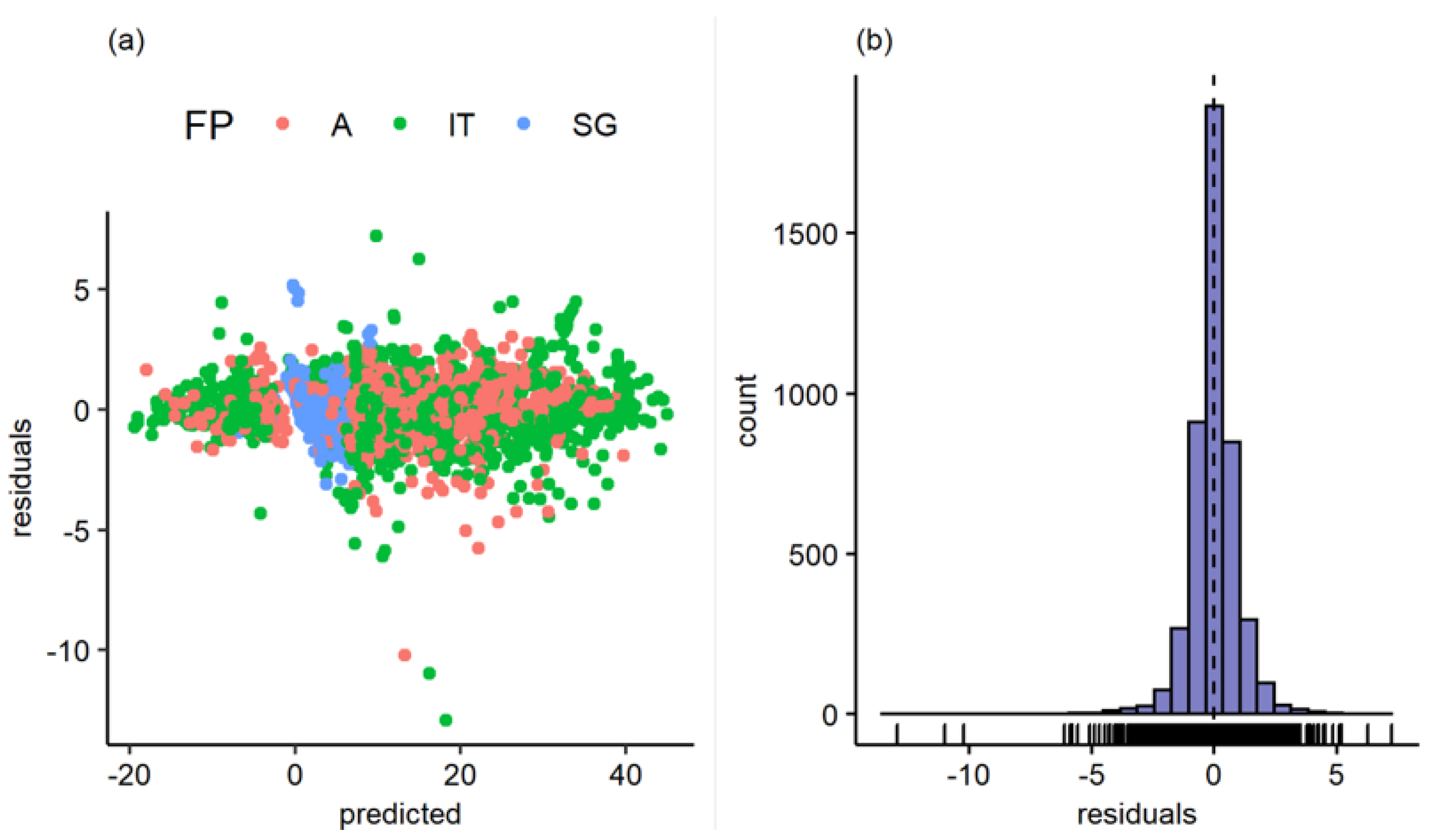
This relative error is similar to models such as the one proposed by Zhang et al. [10] or correlations such as those by Andritsos, Williams, and Hanratty [47]. The total deviance explained by the model is 99.2%, and the adjusted $R^2$ is 99.1%, which both mean the model already explains the total variance practically in the data and that it will perform adequately in a test sample, as shown both in Figure 9 and

Table 4. MSE and relative error results on the train and test dataset used for the GAM calibrated with the shrinkage approach.

Set	Pattern	MSE	Mean Relative Error (%)
Train	Total	0.9239	11.720
	A	12.404	11.860
	BF	0.1661	1.330
	IT	12.919	10.390
	SG	0.2474	16.290
Test	Total	17.473	11.080
	A	41.118	9.660
	BF	0.2860	2.340
	IT	16.122	10.960
	SG	0.3680	14.020
Deviance Exp.	99.20%	AIC	13,110.21

A: Annular, BF: Bubbly Flow, IT: Intermittent, SG: Segregated.

. The distribution of standardized residuals shown in Figure 10 has no identifiable patterns, and the histogram suggests normality in the residuals, indicating that the model is correctly specified. It has a light skewness to the left, meaning the model can sometimes underpredict the pressure drop. However, this is on a small subset of the whole sample and should not be a concern considering the model’s predictive capability. Furthermore, the model performs adequately both in downward and upward cases. Residuals which are used in Figure 10a,b are defined using the standardized residuals expression:

$$Residuals={\displaystyle \frac{Y_{obs}^i-Y_{pred}^i}{\sqrt{{\displaystyle \frac{{\sum }_{i=1}^n{Y}_{obs}^i-Y_{pred}^i}{n-1}}}}}$$

(31)

This model’s critical weakness is using most of the predictors, although some of them are removed considering the tool proposed by Marra and Wood [46] for a total of 19 dimensionless numbers as predictors in the GAM with a double penalty. Considering the four different flow patterns, 76 different splines need to be calibrated for the trained model. This situation makes interpretability difficult because it is required to review all the significant predictors’ responses. Since the appeal of the GAM is a compromise between predictive capacity and interpretability, this is a weakness that should be addressed.

The first approach to reduce the number of features in the model considered analyzing the information in Table 4, specifically, the relative error in each flow pattern. This table suggests that the model is beneficial to predict the bubbly flow. Therefore, the proposed trade-off would reduce the model’s capability to predict bubbly flow and reduce the number of features, which should improve the interpretability and confidence interval of each spline. For this purpose, the model was trained to ignore bubbly flow cases, assuming they were intermittent flow cases since intermittent flow is the most prevalent in the database. This assumption means that the model does not distinguish between bubbly flow and intermittent flow on a dataset. The hypothesis is that if the model can predict the pressure drop in intermittent flow cases correctly, then it will continue to predict the bubbly flow cases correctly in a test dataset. This approach’s advantage was the reduction from 76 initial predictors to 57 predictors (i.e., 19 are immediately removed) before the double penalty regularization is done since a whole flow pattern was removed from the training process. The results of the model without bubbly flow are shown in

Table 5. Results on train and test set for the GAM without bubbly flow training.

Set	Pattern	MSE	Mean Relative Error (%)
Train	Total	0.983	12.347
	A	10.590	11.028
	BF	1.335	3.579
	IT	12.584	9.221
	SG	0.4062	19.269
Test	Total	1.237	12.926
	A	12.971	9.420
	BF	13.553	4.413
	IT	15.585	10.557
	SG	0.6087	19.977
Deviance Exp.	99.20%	AIC	13,562.47

A: Annular, BF: Bubbly Flow, IT: Intermittent, SG: Segregated.

.

Table 5 shows that a GAM that predicts correctly intermittent flow can still have excellent bubbly flow performance. The AIC increased only by 3.3%, but only 50 splines remained to be interpreted after double penalty regularization, which is statically relevant with a 5% significance level. Nevertheless, 50 splines are still much information to consider, but the model could significantly reduce predictive capacity seeking to prune more. The problem with this model is that it starts predicting less accurately segregated flow pattern cases, as shown in Table 5, where the MSE of the segregated flow is the smallest in this case.

Another way to improve each flow pattern’s relative error is by calibrating a GAM for each flow pattern using all the dimensionless numbers and the double penalty approach. The problem with this approach is that it is more sensible to flow pattern misclassification since the splines are not built based on the other flow patterns but only on the application. Furthermore, since 4% relative error is still acceptable for bubbly flow, only three models were constructed, and the intermittent flow model was used to predict bubbly flow cases. However, the results of the three models combined on the same train and test datasets are the following:

As shown in

Table 6. Results on train and test set by using three models, one for annular, one for stratified, and one for intermittent.

Set	Pattern	MSE	Mean Relative Error (%)
Train	A	0.9160	9.842
	BF	13.517	3.593
	IT	12.828	9.288
	SG	0.2522	17.401
Test	A	67.762	13.042
	BF	13.400	4.246
	IT	15.485	10.389
	SG	0.3411	17.623

A: Annular, BF: Bubbly Flow, IT: Intermittent, SG: Segregated.

, using a different model for each flow pattern has similar results to the best model found. However, as seen in the MSE of the annular flow pattern, it can have worse results on a test data set since it has fewer data to train each model. Furthermore, statistical metrics such as AIC are not comparable to previous models since the training samples are different.

5.2. Results of the GAM

This section presents the results that do not distinguish between the intermittent and bubbly flow. The results of the full GAM model with all the flow patterns are shown in the annexes. The results of the methodology that fitted one GAM for each flow pattern are also presented. The statistical significance results of the GAM can be seen in

Table 7. Parametric coefficients of the GAM. The base case is the annular flow pattern, and the bubbly flow is mixed with intermittent flow.

Parametric Coefficients
	Estimate	Std. Error	t Statistic	p-Value
Intercept (A)	6.433	13.185	0.488	0.626
IT	3.749	13.191	0.284	0.776
SG	−9.939	31.325	−0.317	0.751

A: Annular, IT: Intermittent, SG: Segregated.

and

Table 8. Results of the non-parametric tests of the GAM. Estimated degrees of freedom is proportional to the complexity of each spline.

Approximate Significance of Smooth Terms:
Spline	E. dof	R. dof	F Statistic	p-Value	Spline	E. dof	R. dof	F Statistic	p-Value
$s\left(w_G\right)$:A	0.975	9	4.346	<0.0001	$s\left(f_I\right)$:A	4.082	9	11.453	<0.0001
$s\left(w_G\right)$:IT	3.286	9	2.531	<0.0001	$s\left(f_I\right)$:IT	3.730	9	20.569	<0.0001
$s\left(w_G\right)$:SG	0.000	9	0.000	0.4610	$s\left(f_I\right)$:SG	2.798	9	1.648	0.0001
$s\left(R{e}_L\right)$:A	5.499	19	3.505	<0.0001	$s\left(Ft\right)$:A	5.797	9	5.18	<0.0001
$s\left(R{e}_L\right)$:IT	14.410	19	10.184	<0.0001	$s\left(Ft\right)$:IT	5.089	9	5.532	<0.0001
$s\left(R{e}_L\right)$:SG	0.897	16	0.543	0.0009	$s\left(Ft\right)$:SG	0.301	9	0.048	0.1159
$s\left(R{e}_M\right)$:A	10.790	18	23.061	<0.0001	$s\left(Y_{TD}\right)$:A	10.100	17	10.531	<0.0001
$s\left(R{e}_M\right)$:IT	14.220	19	12.224	<0.0001	$s\left(Y_{TD}\right)$:IT	15.630	19	85.988	<0.0001
$s\left(R{e}_M\right)$:SG	10.740	19	5.336	<0.0001	$s\left(Y_{TD}\right)$:SG	1.028	7	7.34	<0.0001
$s\left(W{e}_G\right)$:A	12.710	19	6.471	<0.0001	$s\left(Eo\right)$:A	3.483	5	7.002	<0.0001
$s\left(W{e}_G\right)$:IT	3.498	19	1.065	<0.0001	$s\left(Eo\right)$:IT	4.953	5	150.699	<0.0001
$s\left(W{e}_G\right)$:SG	13.680	18	26.050	<0.0001	$s\left(Eo\right)$:SG	3.967	5	122.387	<0.0001
$s\left(W{e}_L\right)$:A	7.581	18	3.293	<0.0001	$s\left(\chi \right)$:A	0.939	19	0.803	<0.0001
$s\left(W{e}_L\right)$:IT	10.290	19	4.777	<0.0001	$s\left(\chi \right)$:IT	8.757	18	4.911	<0.0001
$s\left(W{e}_L\right)$:SG	0.000	10	0.000	0.5311	$s\left(\chi \right)$:SG	0.000	19	0	0.2248
$s\left(W{e}_M\right)$:A	6.757	9	11.820	<0.0001	$s\left(N_{\mu }\right)$:A	15.690	19	32.64	<0.0001
$s\left(W{e}_M\right)$:IT	4.515	9	6.304	<0.0001	$s\left(N_{\mu }\right)$:IT	12.700	19	101.09	<0.0001
$s\left(W{e}_M\right)$:SG	1.294	8	0.535	0.0149	$s\left(N_{\mu }\right)$:SG	6.823	17	1.929	<0.0001
$s\left(F{r}_G\right)$:A	4.958	19	1.166	<0.0001	$s(L/D)$:A	4.719	6	14.115	<0.0001
$s\left(F{r}_G\right)$:IT	13.680	19	13.242	<0.0001	$s(L/D)$:IT	5.775	6	127.099	<0.0001
$s\left(F{r}_G\right)$:SG	14.750	19	21.040	<0.0001	$s(L/D)$:SG	5.413	6	61.614	<0.0001
$s\left(F{r}_L\right)$:A	14.550	19	13.200	<0.0001	$s\left(\tilde{T}\right)$:A	6.231	9	9.122	<0.0001
$s\left(F{r}_L\right)$:IT	12.270	19	48.426	<0.0001	$s\left(\tilde{T}\right)$:IT	8.404	9	13.493	<0.0001
$s\left(F{r}_L\right)$:SG	4.008	15	1.655	<0.0001	$s\left(\tilde{T}\right)$:SG	6.269	9	51.724	<0.0001
$s\left(f_G\right)$:A	0.671	5	0.407	0.0533	$s\left(\tilde{P}\right)$:A	8.509	15	11.022	<0.0001
$s\left(f_G\right)$:IT	9.217	19	7.514	<0.0001	$s\left(\tilde{P}\right)$:IT	17.080	19	9.897	<0.0001
$s\left(f_G\right)$:SG	4.554	10	9.246	<0.0001	$s\left(\tilde{P}\right)$:SG	9.002	17	11.042	<0.0001
$s\left(f_L\right)$:A	0.000	16	0.000	0.5305
$s\left(f_L\right)$:IT	0.001	15	0.000	0.4237
$s\left(f_L\right)$:SG	1.419	19	0.213	0.0450
R-sq (adj)	99.10%	Deviance Explained		99.10%	Scale Estimated	10.738

A: Annular, IT: Intermittent, SG: Segregated. E.dof: Estimated degrees of freedom of each spline. R.dof: Reference degrees of freedom for each spline.

.

Table 7 and Table 8 show that the parametric terms only comprise the flow pattern, which is a categorical variable. The baseline level is the annular flow pattern; it only changes how the model is interpreted but not the results in any way. The flow patterns are not significant based on their p-values on the response’s mean but are significant as they change the splines’ shape. In Table 8, the need to use a different spline for each flow pattern is revealed since each spline’s estimated degrees of freedom are different for the same dimensionless number. The reference degrees of freedom are the maximum the splines can have. The back-fitting algorithm optimizes the best-estimated degrees of freedom in this range that perform better in theory based on metrics such as generalized cross-validation. The reference degrees of freedom are arbitrarily selected, but they should be large enough to prevent under smoothing, considering that too large degrees of freedom may have computational costs. The p-values are based on the cumulative F distribution, and they are the probability accumulated in the right tail. If this probability is low, it means that the term has a statistically significant non-linear effect on the pressure gradient. In this model, most non-parametric terms significantly affect the response, even after the double penalty approach. So, filtering the variables more could reduce the performance of the model significantly. As can be seen, the adjusted $R^2$ is the same as the deviance, which is a clear indication that most of the variables are necessary to explain the variance in the model. They are also both near the unity and show that the model predicts the pressure gradient.

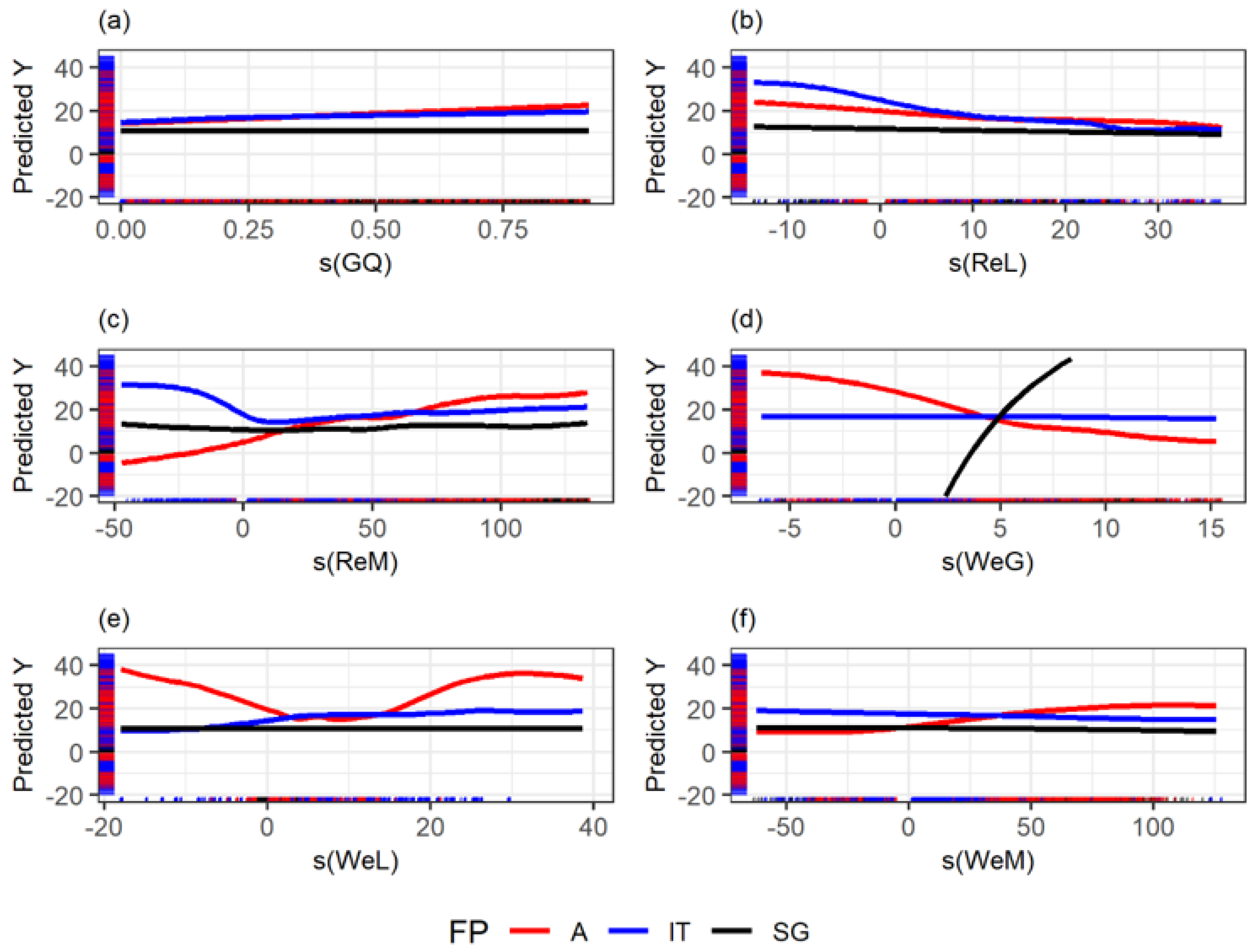
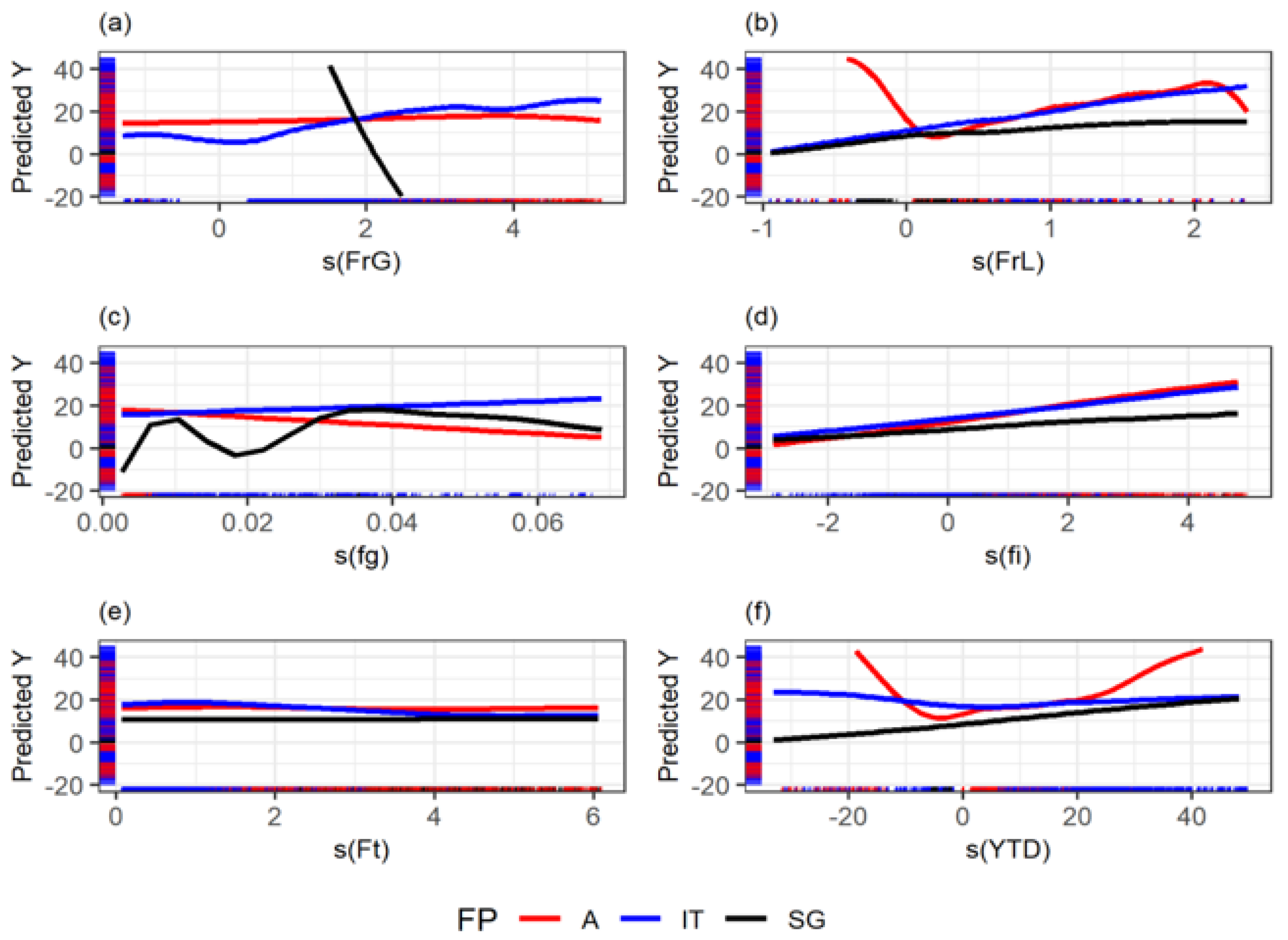
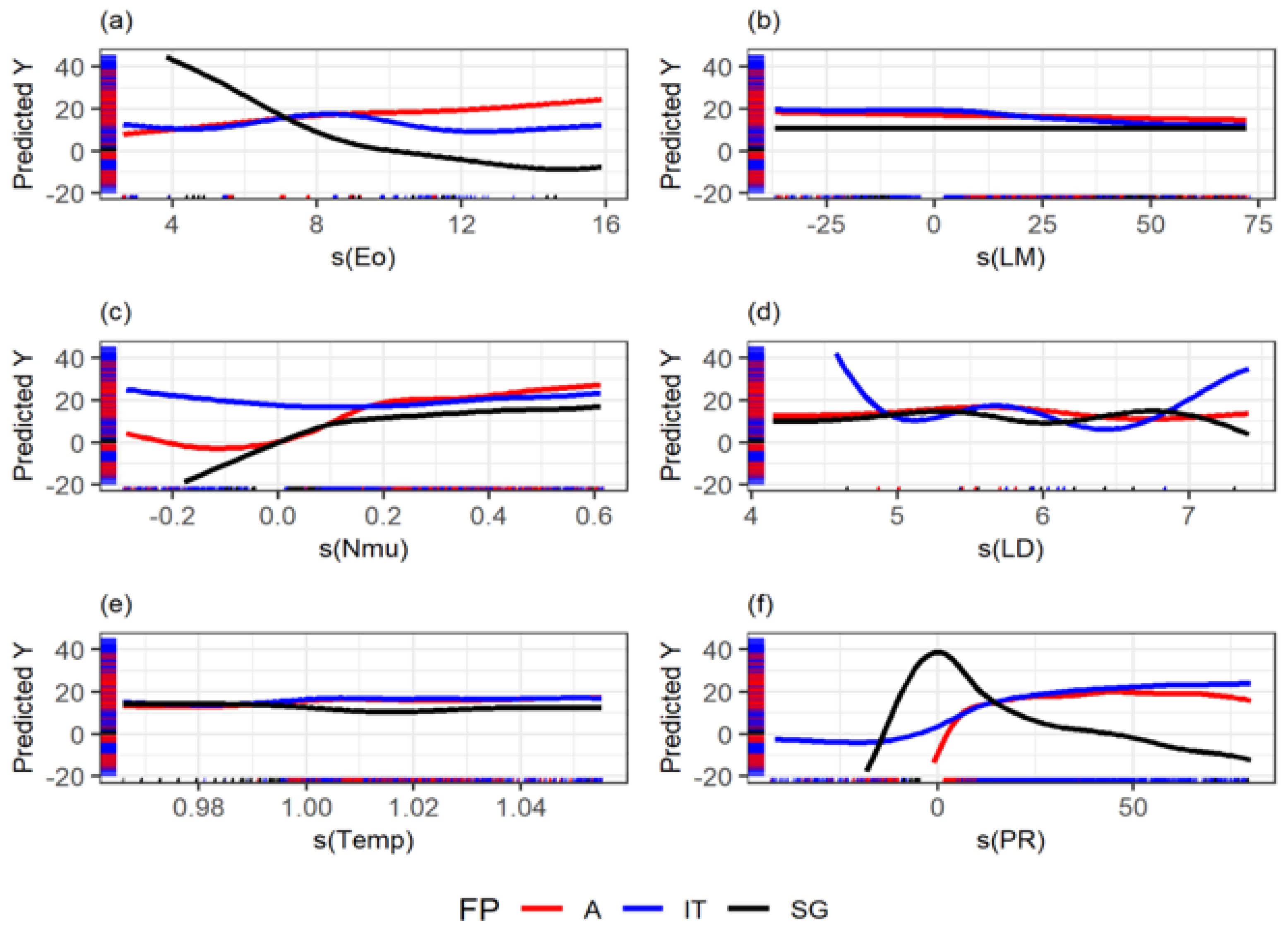
Figure 11, Figure 12 and Figure 13 show the splines of the model. These figures could provide attractive insights since each dimensionless effect on the pressure drop can be compared, considering flow patterns. Figure 11 shows some of the insights that can be drawn from the GAM methodology. For example, it is known that liquid entrainment can have an impact on stratified flow. The gas weber number is related to how liquid droplets can enter the gas phase and start a transition between flow patterns. For example, Zhang, Wang, Sarica, and Brill [10] used a liquid entrainment empirical correlation for stratified flow. This can explain the strong dependence on the gas weber number for the stratified case, as shown in that spline, comparing it to intermittent and annular flow.

The splines shown in Figure 11, Figure 12 and Figure 13 demonstrate the relationship between the cube root of the dimensionless predictors and the cube root of the pressure gradient. The splines are plotted in a window such that they comprise the mean of the dimensionless predictor and two standard deviations. These plots also show the model’s limitations since points outside the showed window should not be predicted with confidence. Nonetheless, all the dimensionless numbers have a large window for prediction.

In some cases, the relations are as expected, such as in the liquid Reynolds, which is inversely proportional to the pressure gradient in annular and intermittent flow. Similar to the single-phase flow case, friction losses decrease in a turbulent flow. However, mixture Reynolds shows the inverse relationship in annular, which can be explained by the gas phase’s drag experienced or the gas’s compressibility, and because the annular flow has the more considerable void fraction typically.

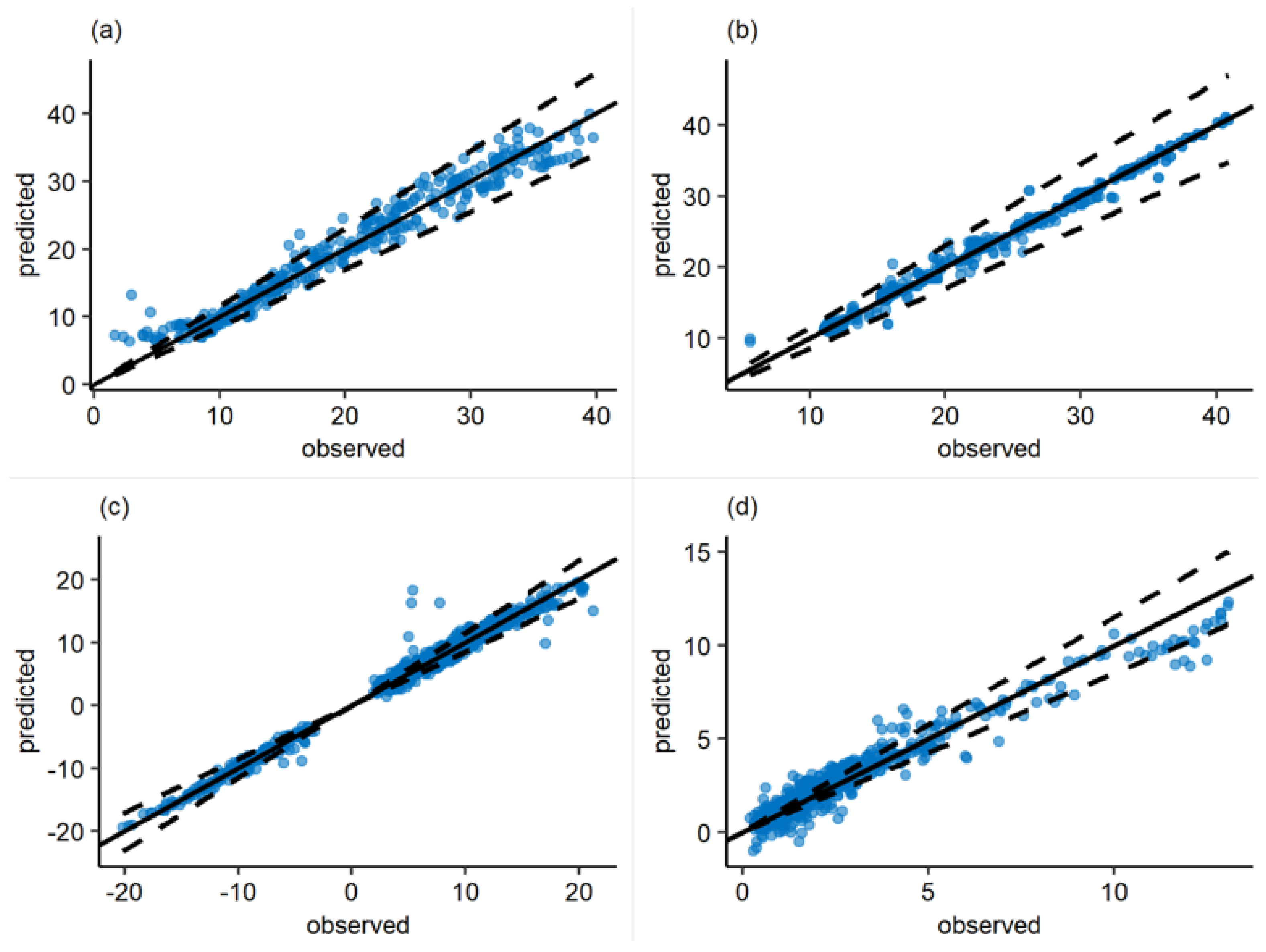
5.3. Performance on the Authors’ Datasets

The predicted vs. observed plot of the model on the data of the most prevalent author of each flow pattern is showed: Rezkallah [39] for annular flow; Aggour [27] for bubbly flow; Kokal [37] for intermittent flow, and Andritsos [31] for stratified flow.

Figure 14 displays the excellent agreement of the model to the authors’ data. Again, stratified flow is the one with the worst performance. It was shown that fitting different GAMs for each flow pattern could solve this problem. Furthermore, stratified flow is the one that can be easier to predict because of the well-defined liquid height so that a hybrid model approach could be used—for example, using a mechanistic model for stratified flow and the GAM for the other flow patterns.

5.4. Performance against Mechanistic and Black-Box Models

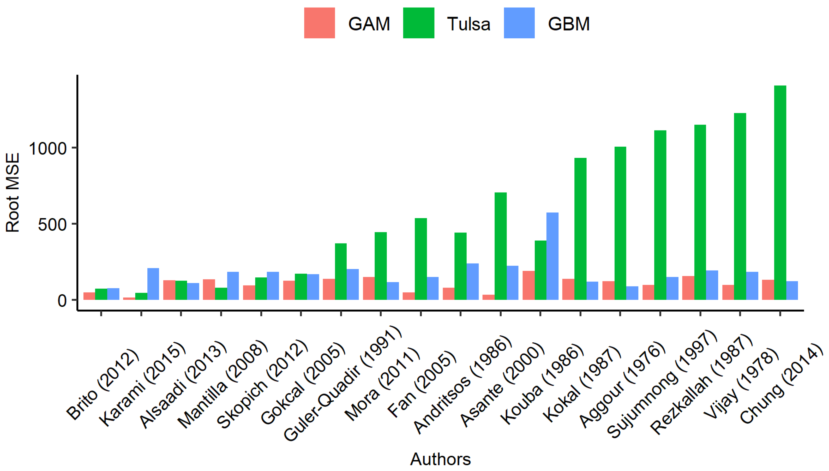
After describing the proposed approach’s prediction capabilities, it was compared in terms of predictive performance against both mechanistic and statistical-machine learning tools. In this regard, the Tulsa Unified Model proposed by Zhang et al. [10], which is a mechanistic model for all types of flow patterns and inclinations, and a gradient boosting model (GBM) approach, which is an application of the work done by Kanin et al. [5] on the database described in Section 3, which is a machine learning model with high predictive capacity were compared with the proposed GAM. Figure 15 shows the mean relative error and mean square error of the three approaches for each dataset recollected.

To calibrate Kanin et al.’s [5] GBM, the R xgboost library was used. It was calibrated by margins following the same sequence as in the original work. Two GBM were built, one using the same predictors as the authors of the model and using the same dimensionless numbers used in this model. The one with more predictors, which uses the dimensionless numbers of this work, is the one with lower test-MSE, so that result is considered.

Figure 15 shows that the GAM has excellent results in all of the author’s datasets, and that results are consistent across the datasets. While the Tulsa model has a problem fitting some of the authors’ results, it can be noted that both the GAM and the GBM are competitive when both are calibrated correctly. Nevertheless, as stated in this document, the GAM offers a greater degree of tools such as p-values and confidence intervals as a risk measure and graphical splines to corroborate the predictors’ effect. Moreover, although the mechanistic model offers much more information about fluid dynamics, it cannot predict the pressure gradient with the same level of accuracy as at both Machine Learning models.

6. Conclusions and Future Work

This study proposed a Generalized Additive Model based on 21 recognized dimensionless numbers to predict the pressure drop of gas–liquid two-phase flow based on 5011 records in the Tulsa Unified Fluid Flow Project (TUFFP) database. The prediction results were satisfactory, obtaining a mean relative error of at most 19.98% for stratified flow and 12.93% for all the data points in a randomly sampled test set. The adjusted $R^2$ was 99.1%, which is the same as the deviance explained in the model. The GAM can also predict bubbly flow with a 4.3% relative error without even being trained to know the flow pattern, assuming the cases are mixed with intermittent flow. A regularization methodology was implemented to reduce the dimensionality, but the number of features did not change significantly. The dimensionless numbers used are probably the simplest ones since they use superficial velocities and nominal diameters.

This approach could be improved considering hybrid model approaches to calculate geometrical considerations such as hydraulic diameters, wetted perimeter, or mean velocities. Using these quantities in the input dimensionless numbers of the GAM should condense the information better and reduce the number of features. Finally, it is restated that GAM can also be used to improve the mechanistic model approach. Replacing closure laws with GAM-based methodologies could give a new dynamism and ideas to propose phenomenological reasons for data behavior.

7. Supporting Information

Based on the model proposed in this paper, we developed an app known as DropTool that is available at the following link: https://droptool.shinyapps.io/Pressure_Drop_App/ (accessed on January 2021). This app describes the GAM model’s central core regarding the experimental data, dimensionless numbers, and method implemented. This app allows the user to estimate the pressure drop based on essential fluid and operation properties for the liquid-gas phase flow. As mentioned above, the model requires the flow pattern, and the user needs to choose from Annular, Bubble, Intermittent, or Segregated flow patterns. DropTool incorporates the tool ProPatt: Probabilistic approach of a flow pattern map for horizontal, vertical, and inclined pipelines, which is based on the work of Amaya-Gómez et al. [11].

References

- Li, X.; Miskimins, J.L.; Hoffman, B.T. A Combined Bottom-hole Pressure Calculation Procedure Using Multiphase Correlations and Artificial Neural Network Models. In Proceedings of the SPE Annual Technical Conference and Exhibition, Amsterdam, The Netherlands, 27–29 October 2014. [Google Scholar] [CrossRef] [Green Version]
- Hagedorn, A.; Brown, K. Experimental Study of Pressure Gradients Occurring During Continuous Two-Phase Flow in Small-Diameter Vertical Conduits. J. Pet. Technol. 1965, 17, 475–484. [Google Scholar] [CrossRef]
- Beggs, D.; Brill, J. A Study of Two-Phase Flow in Inclined Pipes. J. Pet. Technol. 1973, 25, 607–617. [Google Scholar] [CrossRef]
- Xiao, J.J.; Shonham, O.; Brill, J.P. A Comprehensive Mechanistic Model for Two-Phase Flow in Pipelines. In Proceedings of the SPE Annual Technical Conference and Exhibition, New Orleans, LA, USA, 23–26 September 1990. [Google Scholar] [CrossRef]
- Kanin, E.; Osiptsov, A.; Vainshtein, A.; Burnaev, E. A predictive model for steady-state multiphase pipe flow: Machine learning on lab data. J. Pet. Sci. Eng. 2019, 180, 727–746. [Google Scholar] [CrossRef] [Green Version]
- Carrizales, M.J.; Jaramillo, J.E.; Fuentes, D. Prediction of Multiphase Flow in Pipelines: Literature Review. Ing. Cienc. 2015, 11, 213–233. [Google Scholar] [CrossRef] [Green Version]
- Ishii, M.; Hibiki, T. Drift Flux Model. In Thermo-Fluid Dynamics of Two-Phase Flow; Springer: New York, NY, USA, 2011; Chapter 13; pp. 361–395. [Google Scholar] [CrossRef]
- Shi, H.; Holmes, J.A.; Durlofsky, L.J.; Aziz, K.; Diaz, L.R.; Alkaya, B.; Oddie, G. Drift-Flux Modeling of Two-Phase Flow in Wellbores. SPE J. 2005, 10, 24–33. [Google Scholar] [CrossRef]
- Taitel, Y.; Dukler, A.E. A model for predicting flow regime transitions in horizontal and near horizontal gas-liquid flow. AIChE J. 1976, 22, 47–55. [Google Scholar] [CrossRef]
- Zhang, H.Q.; Wang, Q.; Sarica, C.; Brill, J. Unified Model for Gas-Liquid Pipe Flow via Slug Dynamics—Part 1: Model Development. J. Energy Resour. Technol. 2003, 125, 266–273. [Google Scholar] [CrossRef]
- Amaya-Gómez, R.; López, J.; Pineda, H.; Urbano-Caguasango, D.; Pinilla, J.; Ratkovich, N.; Muñoz, F. Probabilistic approach of a flow pattern map for horizontal, vertical, and inclined pipes. Oil Gas Sci. Technol. Rev. IFP Energies Nouv. 2019, 74, 67. [Google Scholar] [CrossRef]
- Ali, N.; Viggiano, B.; Tutkun, M.; Bayoán Cal, R. Cluster-based reduced-order descriptions of two phase flows. Chem. Eng. Sci. 2020, 222, 115660. [Google Scholar] [CrossRef]
- Xie, T.; Ghiaasiaan, S.; Karrila, S. Artificial neural network approach for flow regime classification in gas–liquid–fiber flows based on frequency domain analysis of pressure signals. Chem. Eng. Sci. 2004, 59, 2241–2251. [Google Scholar] [CrossRef]
- Cozin, C.; Vicencio, F.E.C.; de Almeida Barbuto, F.; Morales, R.M.; da Silva, M.; Arruda, L. Two-Phase Slug Flow Characterization Using Artificial Neural Networks. IEEE Trans. Instrum. Meas. 2016, 65, 494–501. [Google Scholar] [CrossRef]
- Gao, Z.K.; Jin, N.D. Characterization of chaotic dynamic behavior in the gas–liquid slug flow using directed weighted complex network analysis. Phys. A Stat. Mech. Its Appl. 2012, 391, 3005–3016. [Google Scholar] [CrossRef]
- Ansari, A.; Sylvester, N.; Sarica, C.; Shoham, O.; Brill, J. A Comprehensive Mechanistic Model for Upward Two-Phase Flow in Wellbores. SPE Prod. Facil. 1994, 9, 143–151. [Google Scholar] [CrossRef] [Green Version]
- Zhang, H.Q.; Wang, Q.; Sarica, C.; Brill, J.P. Unified Model for Gas-Liquid Pipe Flow via Slug Dynamics—Part 2: Model Validation. J. Energy Resour. Technol. 2003, 125, 274–283. [Google Scholar] [CrossRef]
- Hernández, J.; Valencia, C.; Ratkovich, N.; Torres, C.; Muñoz, F. Data driven methodology for model selection in flow pattern prediction. Heliyon 2019, 5, e02718. [Google Scholar] [CrossRef] [Green Version]
- Mohammadi, S.; Papa, M.; Pereyra, E.; Sarica, C. Genetic algorithm to select a set of closure relationships in multiphase flow models. J. Pet. Sci. Eng. 2019, 181, 106224. [Google Scholar] [CrossRef]
- James, G.; Witten, D.; Hastie, T.; Tibshirani, R. An Introduction to Statistical Learning: With Applications in R; Springer Texts in Statistics; Springer: New York, NY, USA, 2013. [Google Scholar]
- Hastie, T.; Tibshirani, R. Generalized Additive Models: Some Applications. J. Am. Stat. Assoc. 1987, 82, 371–386. [Google Scholar] [CrossRef]
- Petalas, N.; Aziz, K. A Mechanistic Model for Multiphase Flow in Pipes. J. Can. Pet. Technol. 2000, 39. [Google Scholar] [CrossRef]
- Ozbayoglu, E.; Ozbayoglu, M. Estimating Flow Patterns and Frictional Pressure Losses of Two-Phase Fluids in Horizontal Wellbores Using Artificial Neural Networks. Pet. Sci. Technol. 2009, 27, 135–149. [Google Scholar] [CrossRef]
- Wood, S. Generalized Additive Models: An Introduction with R; Chapman and Hall/CRC: Boca Raton, FL, USA, 2006. [Google Scholar]
- Alsaadi, Y. Liquid Loading in Highly Deviated Gas Wells. Master’s Thesis, The University of Tulsa, Tulsa, OK, USA, 2013. [Google Scholar]
- Wood, S. Thin plate regression splines. J. R. Stat. Soc. Ser. B (Stat. Methodol.) 2003, 65, 95–114. [Google Scholar] [CrossRef]
- Aggour, M. Hydrodynamics and Heat Transfer in Two-Phase Two-Component Flows. Ph.D. Thesis, University of Manitoba, Winnipeg, MB, Canada, 1978. [Google Scholar]
- Brito, R. Effect of Medium Oil Viscosity on Two-Phase Oil-Gas Flow Behavior in Horizonal Pipes. Master’s Thesis, The University of Tulsa, Tulsa, OK, USA, 2012. [Google Scholar]
- Fan, Y. An Investigation of Low Liquid Loading Gas-Liquid Stratified Flow in Near-Horizontal Pipes. Ph.D. Thesis, The University of Tulsa, Tulsa, OK, USA, 2005. [Google Scholar]
- Mantilla, I. Mechanistic Modeling of Liquid Entrainment in Gas in Horizontal Pipes. Ph.D. Thesis, The University of Tulsa, Tulsa, OK, USA, 2008. [Google Scholar]
- Andritsos, N. Effect of Pipe Diameter and Liquid Viscosity on Horizontal Stratified Flow. Ph.D. Thesis, University of Illinois at Urbana-Champaign, Urbana, IL, USA, 1986. [Google Scholar]
- Asante, B. Multiphase Transport of Gas and Low Loads of Liquids in Pipelines. Ph.D. Thesis, University of Calgary, Calgary, AB, Canada, 2000. [Google Scholar]
- Chung, S.; Pereyra, E.; Sarica, C.; Soto, G.; Alruhaimani, F.; Kang, J. Effect of high oil viscosity on oil-gas flow behavior in vertical downward pipes. In Proceedings of the 10th North American Conference on Multiphase Production Technology, Banff, AB, Canada, 8–10 June 2016. BHR-2016-259. [Google Scholar]
- Gokcal, B. An Experimental and Theoretical Investigation of Slug Flow for High Oil Viscosity in Horizontal Pipes. Ph.D. Thesis, The University of Tulsa, Tulsa, OK, USA, 2008. [Google Scholar]
- Güler-Quadir, N. Two-Phase Pressure Drop and Holdup in Flows Through Large Diameter Vertical Tubing. Ph.D. Thesis, The University of Tulsa, Tulsa, OK, USA, 1991. [Google Scholar]
- Karami Mirazizi, H. Low Liquid Loading Three-Phase Flow and Effects of MEG on Flow Behavior. Ph.D. Thesis, The University of Tulsa, Tulsa, OK, USA, 2015. [Google Scholar]
- Kokal, S.L. An Experimental Study of Two Phase Flow in Inclined Pipes. Ph.D. Thesis, University of Calgary, Calgary, AB, Canada, 1987. [Google Scholar] [CrossRef]
- Kouba, G. Horizontal Slug Flow Modelling and Metering. Ph.D. Thesis, The University of Tulsa, Tulsa, OK, USA, 1986. [Google Scholar]
- Rezkallah, K. Heat Transfer and Hydrodynamics in Two-Phase Two-Component Flow in a Vertical Tube. Ph.D. Thesis, University of Manitoba, Winnipeg, MB, Canada, 1987. [Google Scholar]
- Skopich, A. Experimental Study of Surfactant Effect on Liquid Loading in 2-in and 4-in Diameter Vertical Pipes. Master’s Thesis, The University of Tulsa, Tulsa, OK, USA, 2012. [Google Scholar]
- Sujumnong, M. Heat Transfer Pressure Drop and Void Fraction in Two Phase, Two-Component Flow in a Vertical Tube. Ph.D. Thesis, University of Manitoba, Winnipeg, MB, Canada, 1997. [Google Scholar]
- Vijay, M. A Study of Heat Transfer in Two-Phase Two-Component Flow in Vertical Tube. Ph.D. Thesis, University of Manitoba, Winnipeg, MB, Canada, 1977. [Google Scholar]
- Graham, D.; Kopke, H.; Wilson, M.; Yashar, D. An Investigation of Void Fraction in the Stratified/Annular Flow Regions in Smooth, Horizontal Tubes; Technical Report; Part of ACRC Project 74; Air Conditioning and Refrigeration Center, College of Engineering, University of Illinois at Urbana-Champaign: Urbana, IL, USA, 1999. [Google Scholar]
- Brauner, N.; Maron, D. Identification of the range of ‘small diameters’ conduits, regarding two-phase flow pattern transitions. Int. Commun. Heat Mass Transf. 1992, 19, 29–39. [Google Scholar] [CrossRef]
- Al-Safran, E.; Kora, C.; Sarica, C. Prediction of slug liquid holdup in high viscosity liquid and gas two-phase flow in horizontal pipes. J. Pet. Sci. Eng. 2015, 133, 566–575. [Google Scholar] [CrossRef]
- Marra, G.; Wood, S. Practical variable selection for generalized additive models. Comput. Stat. Data Anal. 2011, 55, 2372–2387. [Google Scholar] [CrossRef]
- Andritsos, N.; Williams, L.; Hanratty, T. Effect of liquid viscosity on the stratified-slug transition in horizontal pipe flow. Int. J. Multiph. Flow 1989, 15, 877–892. [Google Scholar] [CrossRef]
Figure 1.
Piecewise linear regression fit on the regression of Gas Velocity to predict Pressure Gradient. Using the data of Alsaadi [25].
Figure 2.
Illustrative shape of the flow patterns used in this work. (a) Bubbly Flow. (b) Intermittent Flow. (c) Segregated Flow. (d) Annular Flow.
Figure 3.
Distribution of phases in the database, (a) Liquids, and (b) Gases.
Figure 4.
Distributions of essential variables in the database. The dotted line corresponds with the sample’s mean.
Figure 5.
Distribution of the inclinations of the pipe in the database.
Figure 6.
Distribution of some of the dimensionless numbers presented in Table 3. Note: Reynolds and Froude are calculated for the liquid phase.
Figure 7.
Distributions of Response Variable for Regression. (a) Histogram of pressure loss. (b) Histogram of transformed response.
Figure 8.
Scheme of the Proposed methodology.
Figure 9.
Results of the best model using double penalty regularization and all the dimensionless numbers proposed. A: Annular, BF: Bubbly Flow, IT: Intermittent, SG: Segregated. (a): Observed vs. Predicted plot on all the datasets with 15% error lines. (b): Observed vs. Predicted plot on a 500-points sample taken as a validation set, with 15% error lines.
Figure 10.
Distribution of residuals of GAM with double penalty regularization. A: Annular, BF: Bubbly Flow, IT: Intermittent, SG: Segregated. (a) Predicted vs. residuals scatterplot. The discontinuity between the two clusters in this plot is the division between upward and downward cases. (b) Histogram of residuals.
Figure 11.
Splines of the cube root of the dimensionless numbers against the pressure gradient’s centered cube root. A: Annular, IT: Intermittent, SG: Segregated. (a): Gas Quality. (b): Liquid Reynolds. (c): Mixture Reynolds. (d): Gas Weber. (e): Liquid Weber (f): Gas Weber.
Figure 12.
Splines of the cube root of the dimensionless numbers against the pressure gradient’s centered cube root. A: Annular, IT: Intermittent, SG: Segregated. (a): Gas Froude. (b): Liquid Froude. (c): Gas friction factor. (d): Interfacial friction factor. (e): Froude Rate. (f): Y Taitel and Dukler parameter.
Figure 13.
Splines of the cube root of the dimensionless numbers against the pressure gradient’s centered cube root. A: Annular, IT: Intermittent, SG: Segregated. (a): Eötvös Number. (b): Lockhart–Martinelli parameter. (c): Viscous number. (d): Length diameter ratio. (e): Dimensionless Temperature. (f): Dimensionless Pressure.
Figure 14.
Observed vs. predicted plot with 15% error lines for the four authors mentioned. (a): Rezkallah [39] (6.868% relative error). (b): Aggour [27] (2.691% relative error). (c): Kokal [37] (13.05% relative error). (d): Andritsos [31] (17.04% relative error).
Figure 15.
Model comparison using root mean square error for each author in the database. For the ML models, an out-of-sample test is used.