
A New Method of Quantitatively Evaluating Fracability of Tight Sandstone Reservoirs Using Geomechanics Characteristics and In Situ Stress Field

Abstract
:1. Introduction
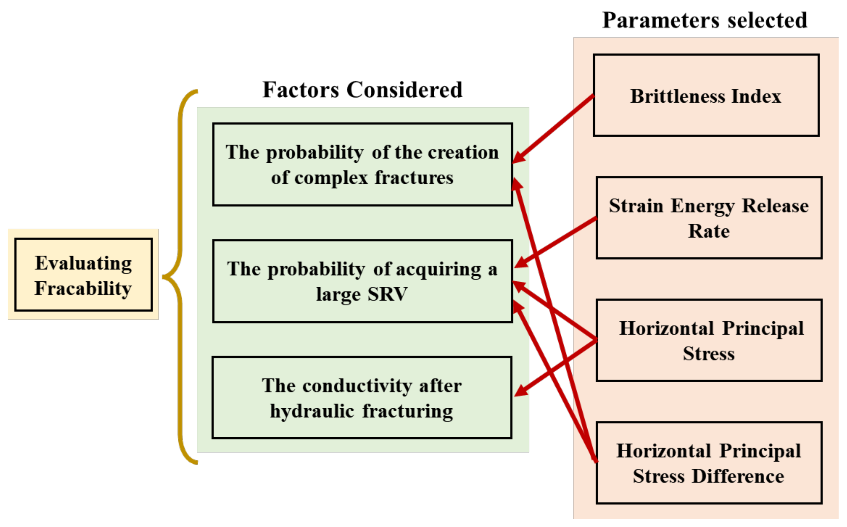
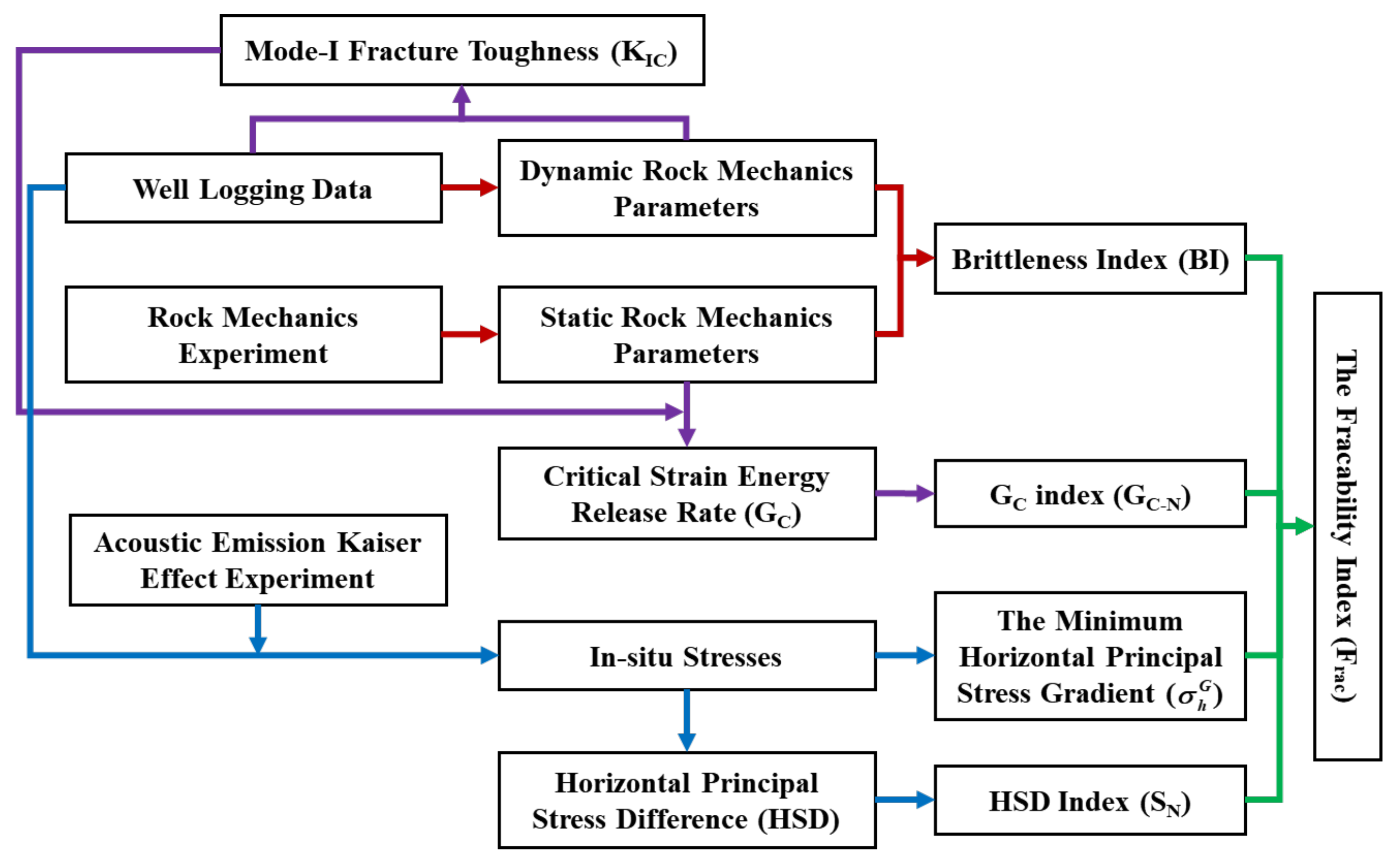
2. Analysis and Calculation of Fracability Evaluation Parameters
2.1. Brittleness Index
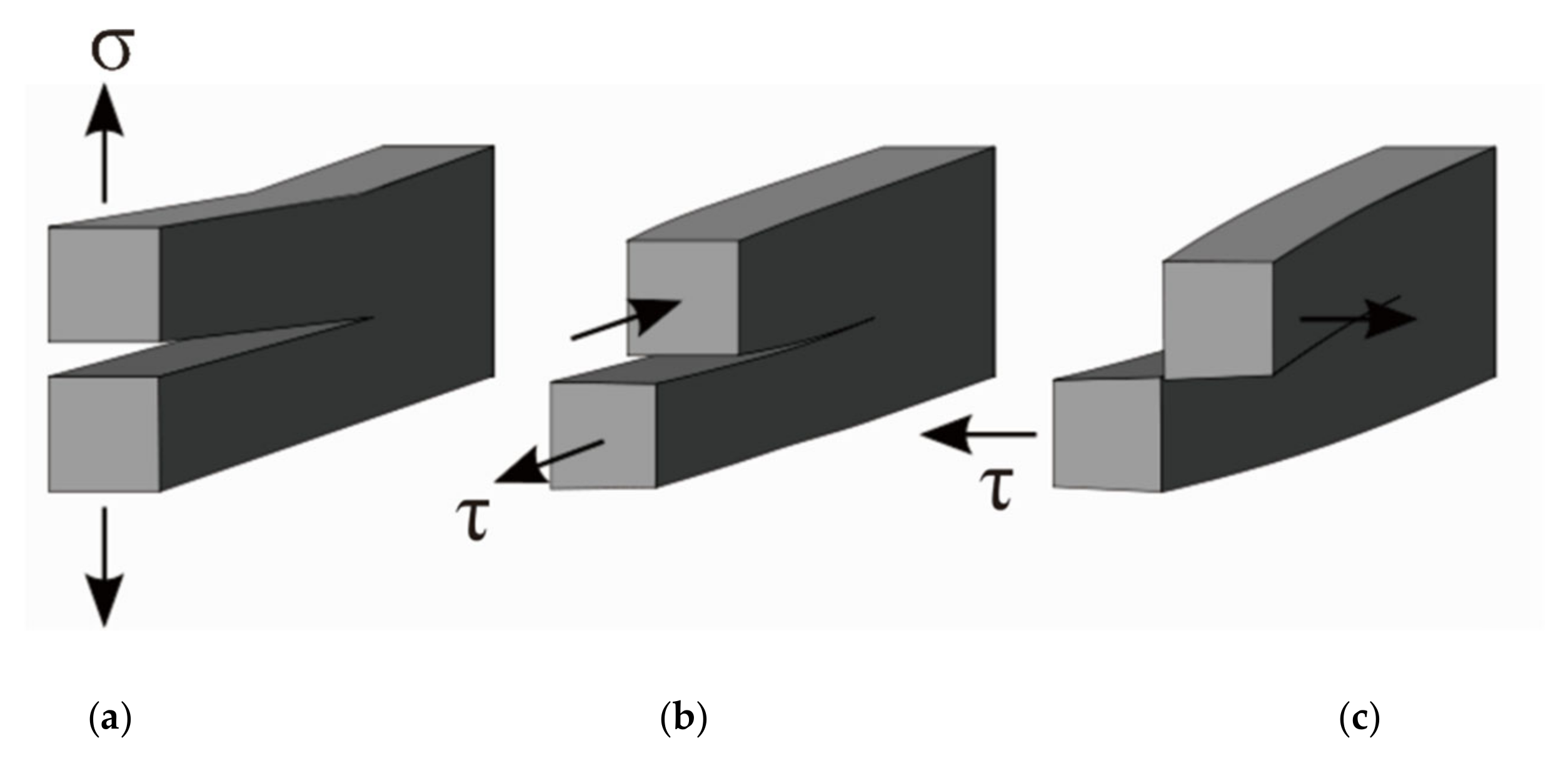
2.2. Strain Energy Release Rate
2.3. Minimum Horizontal Principal Stress and Horizontal Principal Stress Difference
2.3.1. Horizontal Principal Stress
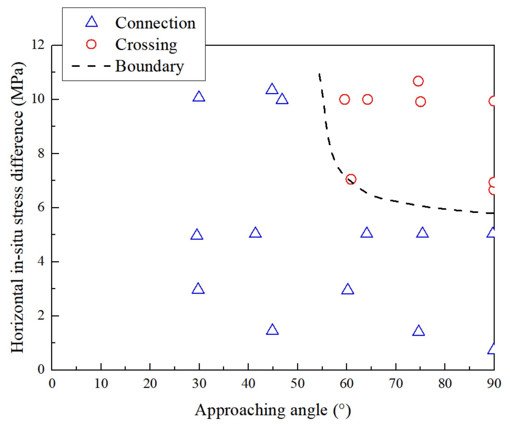
2.3.2. The Effect of Horizontal Principal Stress Difference
3. New Model for Fracability Evaluation
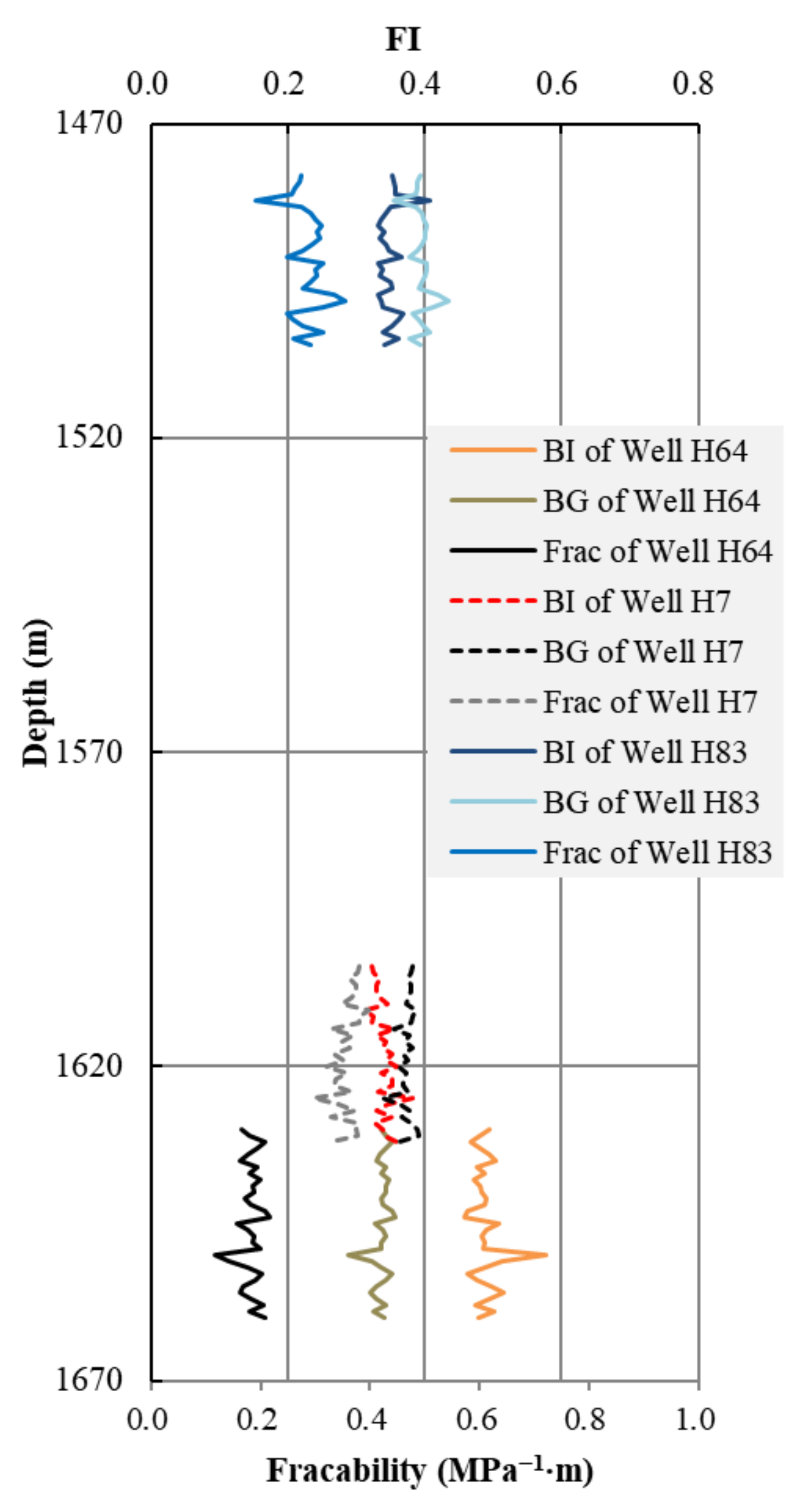
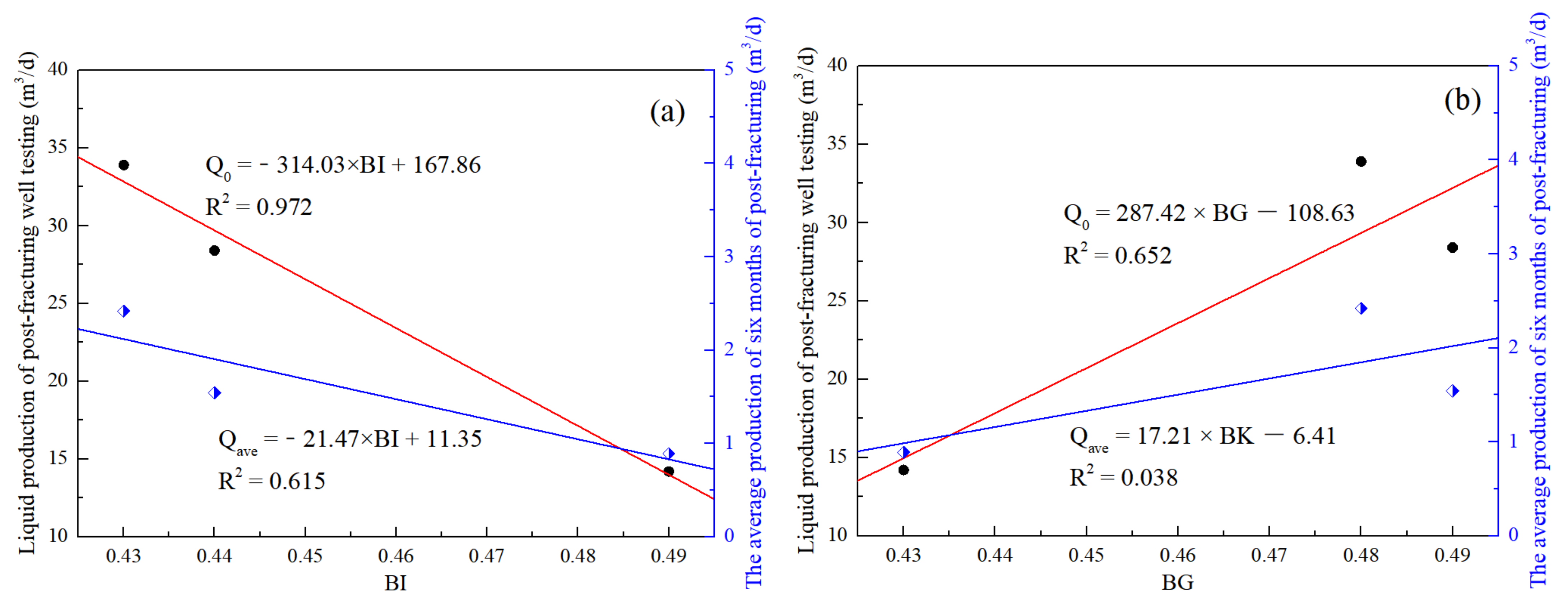
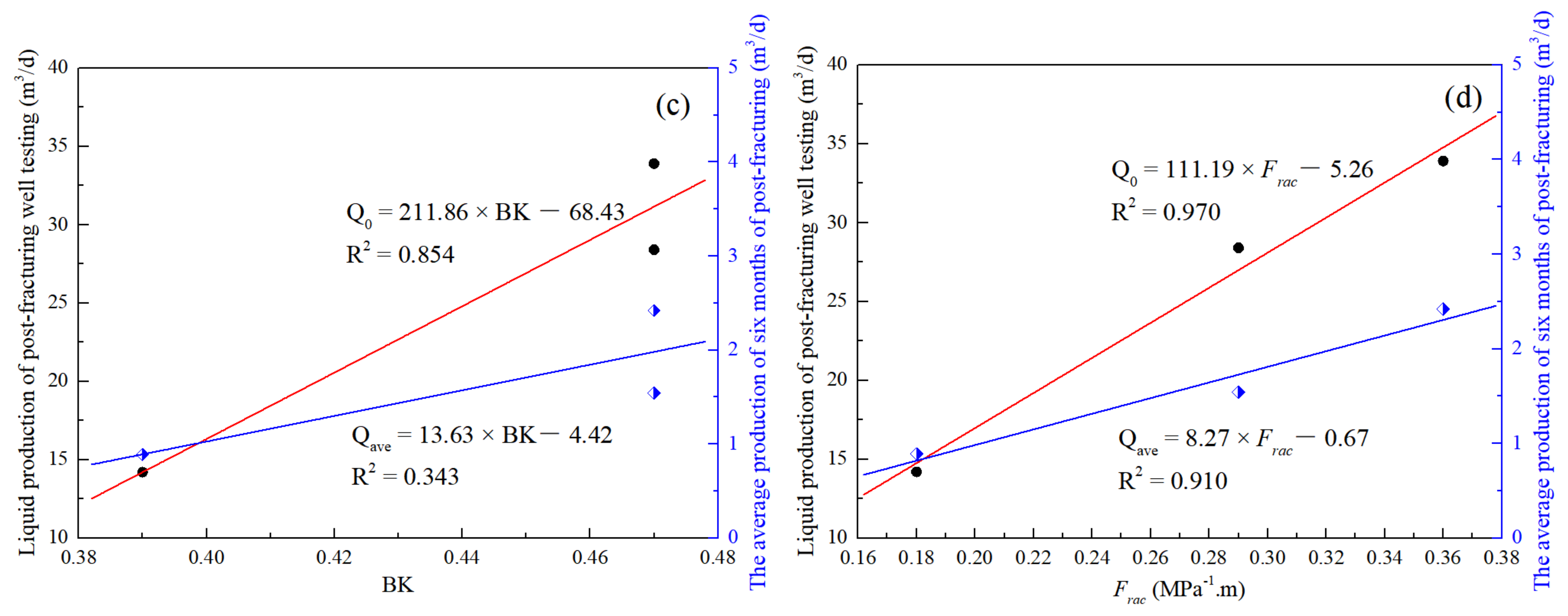
4. Case Study and Comparative Analysis
- (1)
- Type-I: Frac ≥ 0.3 MPa−1∙m. For this type, there was a high probability of obtaining a complex fracture network, a greater SRV, and high conductivity. The fracability was ranked high.
- (2)
- Type-II: 0.22 MPa−1∙m ≤ Frac < 0.3 MPa∙m. For this type, there was an intermediate probability of obtaining a complex fracture network and a greater SRV. The fracability was ranked intermediate.
- (3)
- Type-III: Frac < 0.22 MPa−1∙m. For this type, it was difficult to obtain a complex fracture network and a greater SRV. The fracability was ranked low and hydraulic fracturing is not advised for this type of reservoirs.
5. Conclusions
Author Contributions
Funding
Conflicts of Interest
References
- Sun, J.M.; Han, Z.L.; Qin, R.B.; Zhang, J.Y. Log evaluation method of fracturing performance in tight gas reservoir. Acta Pet. Sin. 2015, 36, 74–80. [Google Scholar]
- Li, Q.H.; Chen, M.; Jin, Y.; Wang, F.P.; Hou, B.; Zhang, B.W. Indoor evaluation method for shale brittleness and improvement. Chin. J. Rock Mech. Eng. 2012, 31, 1680–1685. [Google Scholar]
- Jin, X.; Shah, S.N.; Roegiers, J.C.; Zhang, B. An integrated petrophysics and geomechanics approach for fracability evaluation in shale reservoirs. SPE J. 2015, 20, 518–526. [Google Scholar] [CrossRef]
- Wang, X.; Ge, H.; Wang, D.; Wang, J.; Chen, H. A comprehensive method for the fracability evaluation of shale combined with brittleness and stress sensitivity. J. Geophys. Eng. 2017, 14, 1420–1429. [Google Scholar] [CrossRef] [Green Version]
- Bai, M. Why are brittleness and fracability not equivalent in designing hydraulic fracturing in tight shale gas reservoirs. Petroleum 2016, 2, 1–19. [Google Scholar] [CrossRef] [Green Version]
- Shahbazi, A.; Monfared, M.S.; Thiruchelvam, V.; Fei, T.K.; Babasafari, A.A. Integration of knowledge-based seismic inversion and sedimentological investigations for heterogeneous reservoir. J. Asian Earth Sci. 2020, 202, 104541. [Google Scholar] [CrossRef]
- Soleimani, M.; Jodeiri Shokri, B.; Rafiei, M. Integrated petrophysical modeling for a strongly heterogeneous and fractured reservoir, Sarvak Formation, SW Iran. Nat. Resour. Res. 2017, 26, 75–88. [Google Scholar] [CrossRef]
- Soleimani, M.; Jodeiri Shokri, B. 3D static reservoir modeling by geostatistical techniques used for reservoir characterization and data integration. Environ. Earth Sci. 2015, 74, 1403–1414. [Google Scholar] [CrossRef]
- Chong, K.K.; Grieser, W.V.; Passman, A.; Tamayo, C.H.; Modeland, N.; Burke, B. A Review of Successful Approach Towards Shale Play Stimulation in the Last Two Decades. In Proceedings of the Canadian Unconventional Resources and International Petroleum Conference, Calgary, AB, Canada, 19–21 October 2010. SPE-133874-MS. [Google Scholar]
- Tang, Y.; Xing, Y.; Li, L.Z.; Zhang, B.H.; Jiang, S.X. Influence factors and evaluation methods of the gas shale fracability. Earth Sci. Front. 2012, 19, 356–363. [Google Scholar]
- Yuan, J.L.; Deng, J.G.; Zhang, D.Y.; Li, D.; Yan, W.; Chen, C.; Chen, L.; Chen, Z. Fracability evaluation of shale-gas reservoirs. Acta Pet. Sin. 2013, 34, 523–527. [Google Scholar]
- Zhao, J.Z.; Xu, W.J.; Li, Y.M.; Hu, J.Y.; Li, J.Q. A new method for fracability evaluation of shale-gas reservoirs. Nat. Gas Geosci. 2015, 26, 1165–1172. [Google Scholar]
- Sui, L.; Ju, Y.; Yang, Y.; Yang, Y.; Li, A. A quantification method for shale fracability based on analytic hierarchy process. Energy 2016, 115, 637–645. [Google Scholar] [CrossRef]
- Zhu, Y.; Carr, T.R. Estimation of fracability of the Marcellus shale: A case study from the MIP3H in Monongalia county, West Virginia, USA. In Proceedings of the SPE/AAPG Eastern Regional Meeting, Pittsburgh, PA, USA, 7–11 October 2018. SPE-191818-18ERM-MS. [Google Scholar]
- Wu, J.; Zhang, S.; Cao, H.; Zheng, M.; Sun, P.; Luo, X. Fracability evaluation of shale gas reservoir-A case study in the Lower Cambrian Niutitang formation, northwestern Hunan, China. J. Pet. Sci. Eng. 2018, 164, 675–684. [Google Scholar] [CrossRef]
- Perera, M.S.A.; Sampath, K.H.S.M.; Ranjith, P.G.; Rathnaweera, T.D. Effects of pore fluid chemistry and saturation degree on the fracability of Australian warwick siltstone. Energies 2018, 11, 2795. [Google Scholar] [CrossRef] [Green Version]
- He, R.; Yang, Z.; Li, X.; Li, Z.; Liu, Z.; Chen, F. A comprehensive approach for fracability evaluation in naturally fractured sandstone reservoirs based on analytical hierarchy process method. Energy Sci. Eng. 2019, 7, 529–545. [Google Scholar] [CrossRef]
- Ji, G.; Li, K.; Zhang, G.; Li, S.; Zhang, L. An assessment method for shale fracability based on fractal theory and fracture toughness. Eng. Fract. Mech. 2019, 211, 282–290. [Google Scholar] [CrossRef]
- Zhou, X.; He, F.; Wei, J.G. A New Evaluation Procedure of Rock Fracability Using Cluster Analysis of Well-Logged Petrophysical Properties of Facies. J. Min. Sci. 2020, 56, 753–759. [Google Scholar]
- Li, J.; Li, X.R.; Zhan, H.B.; Song, M.S.; Liu, C.; Kong, X.C.; Sun, L.-N. Modified method for fracability evaluation of tight sandstones based on interval transit time. Pet. Sci. 2020, 17, 477–486. [Google Scholar] [CrossRef] [Green Version]
- Lu, C.; Ma, L.; Guo, J.; Li, X.; Zheng, Y.; Ren, Y.; Yin, C.; Li, J.; Zhou, G.; Wang, J.; et al. Novel method and case study of a deep shale fracability evaluation based on the brittleness index. Energy Explor. Exploit. 2022, 40, 442–459. [Google Scholar] [CrossRef]
- Lutz, S.J.; Hickman, S.; Davatzes, N.; Zemach, E.; Drakos, P.; Robertson-Tait, A. Rock mechanical testing and petrologic analysis in support of well stimulation activities at the Desert Peak Geothermal Field, Nevada. In Proceedings of the 35th Workshop on Geothermal Reservoir Engineering, Stanford, CA, USA, 1–3 February 2010; pp. 373–380. [Google Scholar]
- Holt, R.M.; Fjaer, E.; Nes, O.M.; Alassi, H.T. A shaly look at brittleness. In Proceedings of the 45th US Rock Mechanics/Geomechanics Symposium, San Francisco, CA, USA, 26–29 June 2011. ARMA-11-366. [Google Scholar]
- Enderlin, M.B.; Alsleben, H.; Beyer, J.A. Predicting fracability in shale reservoirs. In Proceedings of the AAPG Annual Convention and Exhibition, Houston, TX, USA, 10–13 April 2011. [Google Scholar]
- Mullen, M.; Enderlin, M. Fracability Index-more than just calculating rock properties. In Proceedings of the SPE Annual Technical Conference and Exhibition, San Antonio, TX, USA, 8–10 October 2012. SPE-159755-MS. [Google Scholar]
- Yuan, J.; Zhou, J.; Liu, S.; Feng, Y.; Deng, J.; Xie, Q.; Lu, Z. An improved fracability-evaluation method for shale reservoirs based on new fracture toughness-prediction models. SPE J. 2017, 22, 1704–1713. [Google Scholar] [CrossRef]
- Grieser, W.V.; Bray, J.M. Identification of production potential in unconventional reservoirs. In Proceedings of the Production and Operations Symposium, Oklahoma City, OK, USA, 31 March–3 April 2007. SPE-106623-MS. [Google Scholar]
- Rickman, R.; Mullen, M.J.; Petre, J.E.; Grieser, W.V.; Kundert, D. A practical use of shale petrophysics for stimulation design optimization: All shale plays are not clones of the Barnett Shale. In Proceedings of the SPE Annual Technical Conference and Exhibition, Denver, CO, USA, 21–24 September 2008. SPE-115258-MS. [Google Scholar]
- Whittaker, B.N.; Singh, R.N.; Sun, G. Rock fracture mechanics. Principles, design and applications. Dev. Geotech. Eng. 1992, 71, 1–21. [Google Scholar]
- Griffith, A.A. The phenomenon of rupture and flow in solids. Phil. Trans. R. Soc. Lond. A 1920, 221, 163–198. [Google Scholar]
- Irwin, G. Analysis of stresses and strains near the end of cracking traversing a plate. J. Appl. Mech. 1957, 24, 361–364. [Google Scholar] [CrossRef]
- Palaniswamy, K.K.W.G. On the problem of crack extension in brittle solids under general loading. Mech. Today 1978, 4, 87–148. [Google Scholar]
- Jin, Y.; Chen, M.; Zhang, X. Determination of fracture toughness for deep well rock with geophysical logging data. Chin. J. Rock Mech. Eng. 2001, 20, 454–456. [Google Scholar]
- Jin, Y.; Yuan, J.; Chen, M.; Chen, K.P.; Lu, Y.; Wang, H. Determination of rock fracture toughness K IIC and its relationship with tensile strength. Rock Mech. Rock Eng. 2011, 44, 621–627. [Google Scholar] [CrossRef]
- Huang, R. A model for predicting formation fracture pressure. J. East China Pet. Inst. 1984, 4, 335–347. [Google Scholar]
- Yu, X.; Wang, Y.; Li, Z. Calculation of horizontal pricipal in-situ stress with acoustic wave method. Acta Pet. Sin. 1996, 17, 59–63. [Google Scholar]
- Holbrook, P. Discussion of a new simple method to estimate fracture pressure gradients. SPE Drill. Completion 1997, 12, 71. [Google Scholar]
- Ge, H.K.; Lin, Y.S.; Ma, S.Z. Modification of Holbrook’s fracture pressure prediction model. Pet. Drill. Tech. 2001, 29, 20–22. [Google Scholar]
- Amadei, B.; Swolfs, H.S.; Savage, W.Z. Gravity-induced stresses in stratified rock masses. Rock Mech. Rock Eng. 1988, 21, 1–20. [Google Scholar] [CrossRef]
- Amadei, B.; Pan, E. Gravitational stresses in anisotropic rock masses with inclined strata. Int. J. Rock Mech. Min. Sci. Geomech. Abstr. 1992, 29, 225–236. [Google Scholar] [CrossRef] [Green Version]
- Higgins, S.M.; Goodwin, S.A.; Bratton, T.R.; Tracy, G.W. Anisotropic stress models improve completion design in the Baxter Shale. In Proceedings of the SPE Annual Technical Conference and Exhibition, Denver, CO, USA, 21–24 September 2008. SPE-115736-MS. [Google Scholar]
- Khan, S.; Ansari, S.; Han, H.; Khosravi, N. Importance of Shale Anisotropy in Estimating In-Situ Stresses and Wellbore Stability Analysis in Horn River Basin. In Proceedings of the Canadian Unconventional Resources Conference, Calgary, AB, Canada, 15–17 November 2011. SPE-149433-MS. [Google Scholar]
- Song, L.; Liu, Z.; Li, C.; Hu, S. Geostress logging evaluation method of tight sandstone based on transversely isotropic model. Acta Pet. Sin. 2015, 36, 707–714. [Google Scholar]
- Lamont, N.; Jessen, F.W. The effects of existing fractures in rocks on the extension of hydraulic fractures. J. Pet. Technol. 1963, 15, 203–209. [Google Scholar] [CrossRef]
- Daneshy, A.A. Hydraulic fracture propagation in the presence of planes of weakness. In Proceedings of the SPE European Spring Meeting, Amsterdam, The Netherlands, 29–30 May 1974. SPE-4852-MS. [Google Scholar]
- Blanton, T.L. An experimental study of interaction between hydraulically induced and pre-existing fractures. In Proceedings of the SPE Unconventional Gas Recovery Symposium, Pittsburgh, PA, USA, 16–18 May 1982. SPE-10847-MS. [Google Scholar]
- Warpinski, N.R.; Teufel, L.W. Influence of geologic discontinuities on hydraulic fracture propagation. J. Pet. Technol. 1987, 39, 209–220. [Google Scholar] [CrossRef]
- Renshaw, C.E.; Pollard, D.D. An experimentally verified criterion for propagation across unbounded frictional interfaces in brittle, linear elastic materials. Int. J. Rock Mech. Min. Sci. Geomech. Abstr. 1995, 32, 237–249. [Google Scholar] [CrossRef]
- Zhou, J.; Chen, M.; Jin, Y.; Zhang, G.Q. Analysis of fracture propagation behavior and fracture geometry using a tri-axial fracturing system in naturally fractured reservoirs. Int. J. Rock Mech. Min. Sci. 2008, 45, 1143–1152. [Google Scholar] [CrossRef]
- Cheng, W.; Jin, Y.; Chen, M.; Xu, T.; Zhang, Y.; Diao, C. A criterion for identifying hydraulic fractures crossing natural fractures in 3D space. Pet. Explor. Dev. 2014, 41, 371–376. [Google Scholar] [CrossRef]
- Cheng, W.; Jin, Y.; Chen, M.; Zhang, Y.; Xi, C.; Hou, B. Experimental investigation on influence of discontinuities on hydraulic fracture propagation in three-dimensional space. Chin. J. Geotech. Eng. 2015, 37, 559–563. [Google Scholar]
- Dou, L.; Yang, M.; Gao, H.; Jiang, D.; Liu, C. Characterization of the dynamic imbibition displacement mechanism in tight sandstone reservoirs using the NMR technique. Geofluids 2020, 2020, 8880545. [Google Scholar] [CrossRef]
- Dou, L.; Xiao, Y.; Gao, H.; Wang, R.; Liu, C.; Sun, H. The study of enhanced displacement efficiency in tight sandstone from the combination of spontaneous and dynamic imbibition. J. Pet. Sci. Eng. 2021, 199, 108327. [Google Scholar] [CrossRef]


| Well | H64 | H7 | H83 | |
|---|---|---|---|---|
| Reservoir physical properties | Porosity (%) | 8.3 | 8.8 | 9.5 |
| Intrinsic permeability (mD) | 0.269 | 0.285 | 0.301 | |
| Saturation of movable fluid (%) | 60.54 | 58.17 | 55.43 | |
| Fracturing operational parameters | Fracturing fluid | Slickwater | Slickwater | Slickwater |
| Amount of sand (m3) | 90.0 | 90.0 | 100.0 | |
| Sand concentrations (%) | 9.0 | 9.5 | 9.1 | |
| Displacement (m3/min) | 1.2 + 3.8 | 1.2 + 3.8 | 1.2 + 3.8 | |
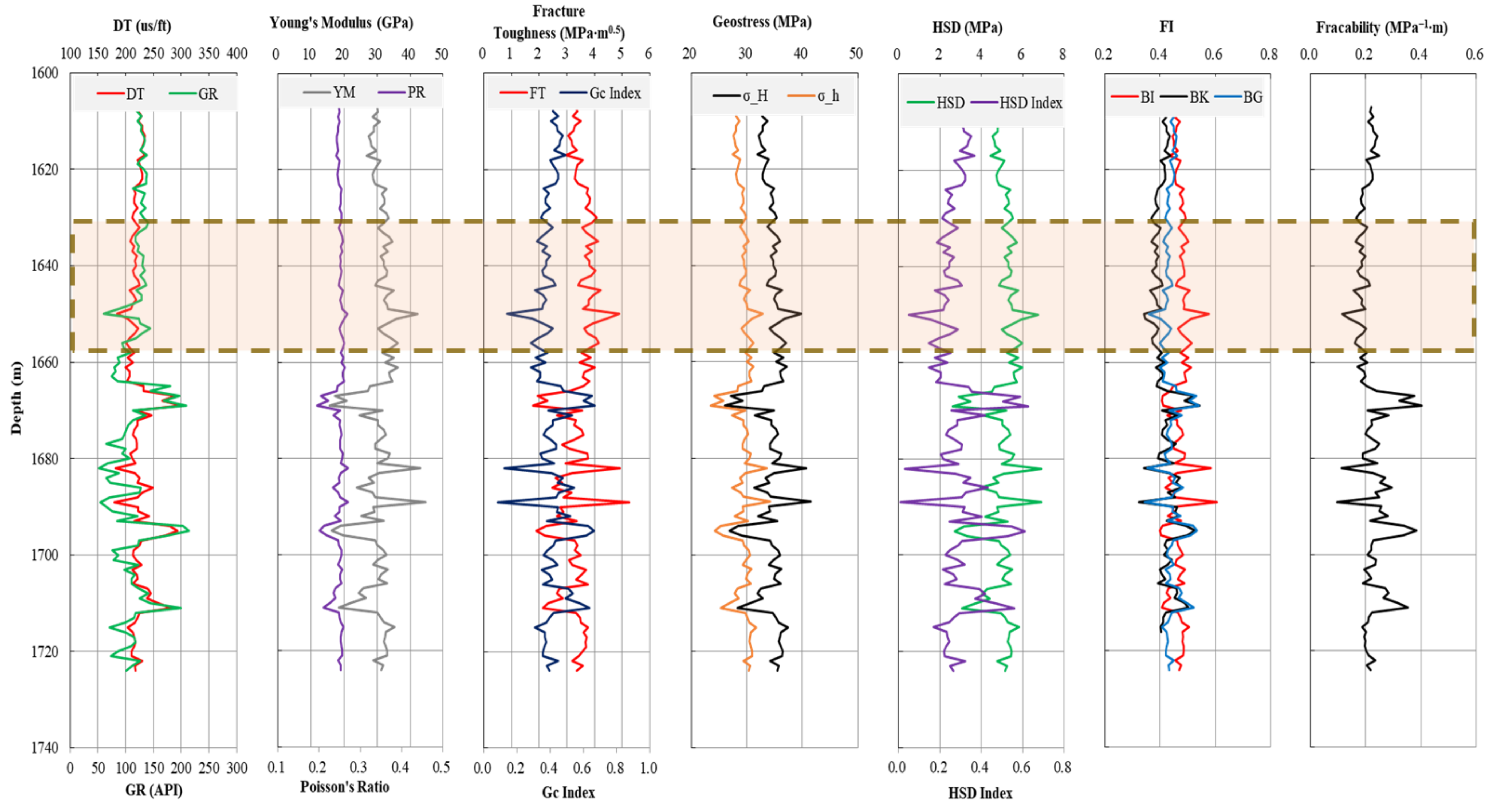
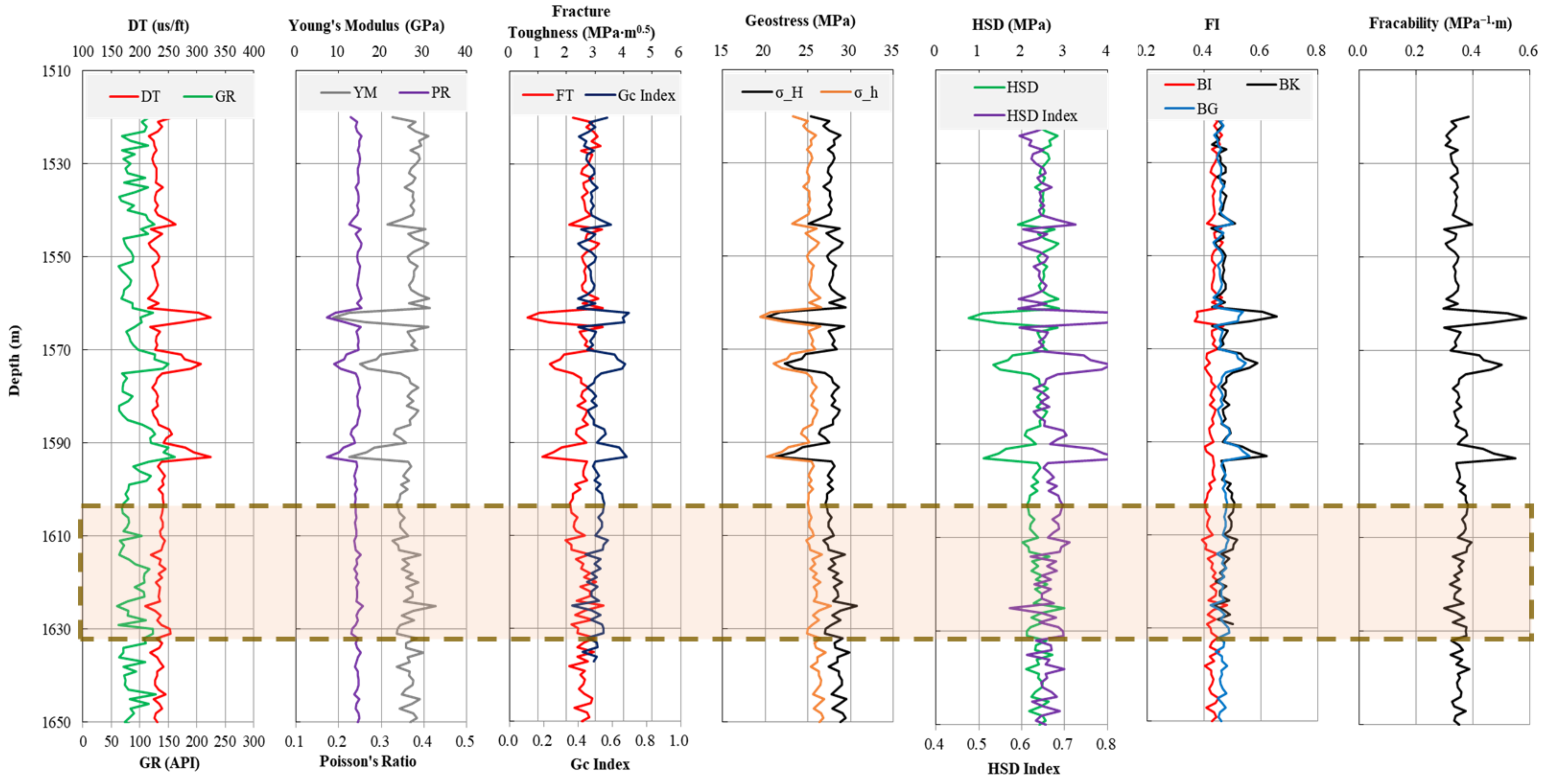
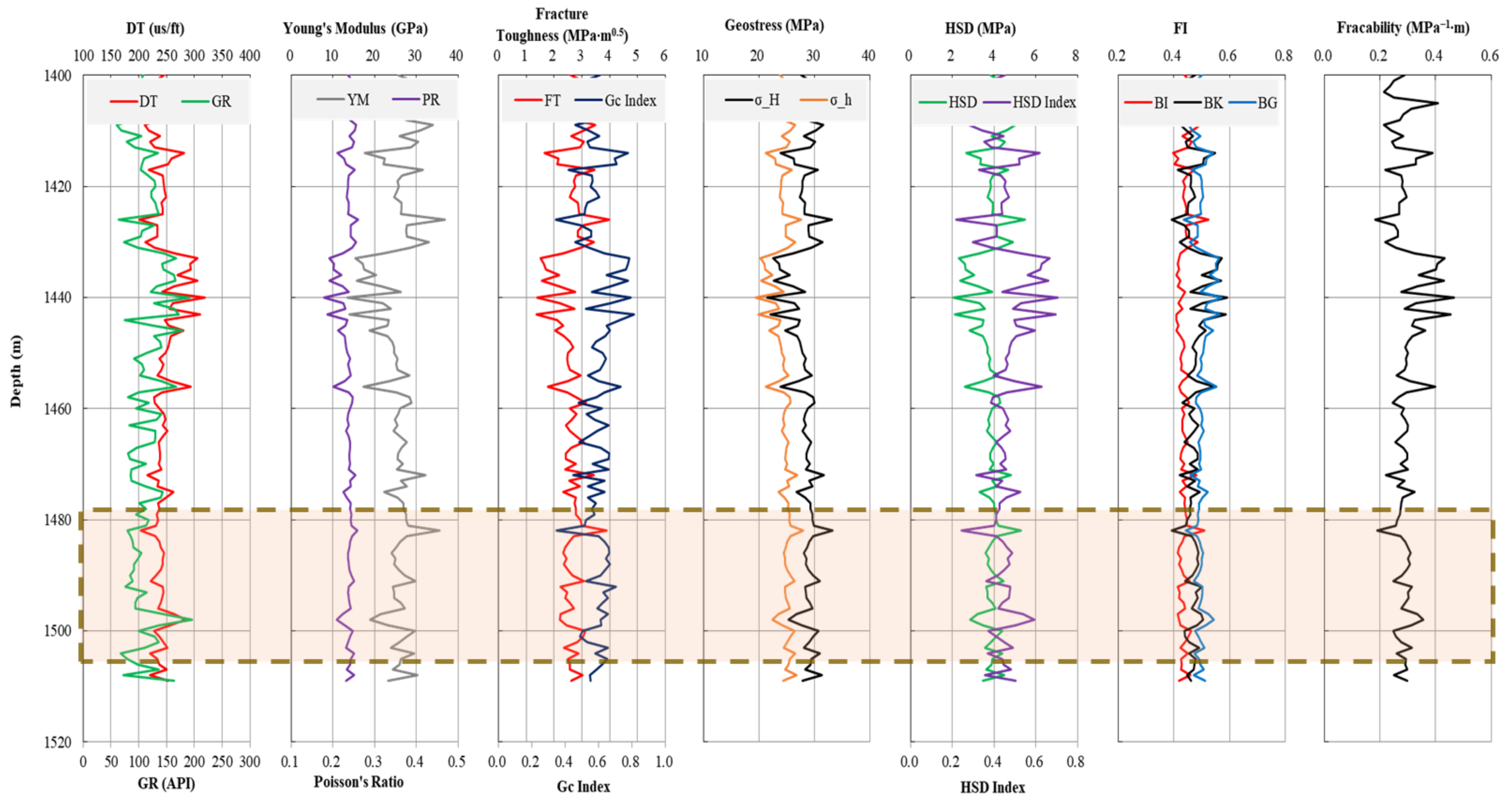
| Fracture height (m) | 1631–1659 | 1605–1631 | 1479–1504 | |
| Fracability | BI | 0.49 | 0.43 | 0.44 |
| BK | 0.39 | 0.47 | 0.47 | |
| BG | 0.43 | 0.48 | 0.49 | |
| Frac (MPa−1·m) | 0.18 | 0.36 | 0.29 | |
| Production | Liquid production of post-fracturing well testing (m3/d), water cut (%) | 14.2, 0 | 33.9, 0 | 28.4, 0 |
| The average production of six months of post-fracturing (m3/d), water cut (%) | 0.89, 58.6% | 2.42, 41.3% | 1.54, 54.8% | |
Publisher’s Note: MDPI stays neutral with regard to jurisdictional claims in published maps and institutional affiliations. |
© 2022 by the authors. Licensee MDPI, Basel, Switzerland. This article is an open access article distributed under the terms and conditions of the Creative Commons Attribution (CC BY) license (https://creativecommons.org/licenses/by/4.0/).
Share and Cite
Dou, L.; Zuo, X.; Qu, L.; Xiao, Y.; Bi, G.; Wang, R.; Zhang, M. A New Method of Quantitatively Evaluating Fracability of Tight Sandstone Reservoirs Using Geomechanics Characteristics and In Situ Stress Field. Processes 2022, 10, 1040. https://0-doi-org.brum.beds.ac.uk/10.3390/pr10051040
Dou L, Zuo X, Qu L, Xiao Y, Bi G, Wang R, Zhang M. A New Method of Quantitatively Evaluating Fracability of Tight Sandstone Reservoirs Using Geomechanics Characteristics and In Situ Stress Field. Processes. 2022; 10(5):1040. https://0-doi-org.brum.beds.ac.uk/10.3390/pr10051040
Chicago/Turabian StyleDou, Liangbin, Xiongdi Zuo, Le Qu, Yingjian Xiao, Gang Bi, Rui Wang, and Ming Zhang. 2022. "A New Method of Quantitatively Evaluating Fracability of Tight Sandstone Reservoirs Using Geomechanics Characteristics and In Situ Stress Field" Processes 10, no. 5: 1040. https://0-doi-org.brum.beds.ac.uk/10.3390/pr10051040