Carbon Emission Reduction Potential in the Finnish Energy System Due to Power and Heat Sector Coupling with Different Renovation Scenarios of Housing Stock

Abstract

In the pursuit of mitigating the effects of climate change the European Union and the government of Finland have set targets for emission reductions for the near future. This study examined the carbon emission reduction potential in the Finnish energy system with power-to-heat (P2H) coupling of the electricity and heat sectors with different housing renovation levels. The measures conducted in the energy system were conducted as follows. Wind power generation was increased in the Finnish power system with 10 increments. For each of these, the operation of hydropower was optimized to maximize the utilization of new wind generation. The excess wind generation was used to replace electricity and heat from combined heat and power production for district heating. The P2H conversion was performed by either 2000 m deep borehole heat exchangers coupled to heat pumps, with possible priming of heat, or with electrode boilers. The housing stock renovated to different levels affected both the electricity and district heating demands. The carbon emission reduction potential of the building renovation measures, and the energy system measures were determined over 25 years. Together with the required investment costs for the different measures, unit costs of emission reductions, €/t-CO₂, were determined. The lowest unit cost solution of different measures was established, for which the unit cost of emission reductions was 241 €/t-CO₂ and the reduced carbon emissions 11.3 Mt-CO₂ annually. Moreover, the energy system measures were found to be less expensive compared to the building renovation measures, in terms of unit costs, and the P2H coupling a cost-efficient manner to increase the emission reductions.

1. Introduction

In the pursuit of limiting climate change the European Union (EU) aims to be an economy with net-zero greenhouse gas emissions by 2050 [1]. The government of Finland has set a national target to be carbon neutral by 2035, which is planned to be achieved with emission reductions and carbon sinks [2]. The total emissions of greenhouse gases (GHGs) in Finland in 2018 were 56.5 Mt-CO₂ equivalent [3] of which the electricity and heat production was responsible for 32% [3,4]. To achieve high emission reductions in these sectors an increase in the share of emission-free generation is likely required. Due to environmental reasons an increase in hydropower production is limited to only capacity increases of existing power plants as they are renovated [5]. Although biomass is often considered not to have any emissions, as it is assumed that the carbon emitted during production is absorbed in the growth of new biomass, the immediate emissions from it are at the same level as peat [6]. However, an advantage of biomass, as for other generation methods based on burning, is its dispatchability. Nuclear power has several advantages compared to other emission-free generation methods, like high constant generation capacity and low cost of produced electricity [7]. The downside of nuclear can be the time required for a new plant to be built; for example, the newest nuclear power plant in Finland, Olkiluoto 3, was intended to begin its operation in 2009 but according to the current estimate it will start in 2022 [8]. Although, it is good to note that at the same time 50 new nuclear power plants have been completed, mainly in Asia, which began their construction after Olkiluoto 3 [9]. So, if the construction time of new plants could be reduced in Finland, also nuclear power could provide rapid emission reductions. However, currently there are no indication of such, and thus for a rapid decarbonization of the energy system, an increase in the share of wind and solar power can be expected. For example, Finnish Energy expects in their vision for the energy production in Finland in 2050 [10] that wind power covers 13% of the total electricity demand. In 2018 wind power production covered already 7% of the total demand [4] and both its installed capacity and annual production have increased rapidly in recent years [11]. Moreover, according to [7] onshore wind power production had the lowest production cost of electricity in Finland and less than half the one compared to solar power. Thus, wind generation was here expected to be an effective manner to achieve emission reductions.

As wind generation is an intermittent energy source, achieving a high share of production from it is likely to require an installation of a significant over capacity [12]. This results in periods with high excess wind power production, which might need to be curtailed. To avoid curtailment and to increase the utilization of wind power the excess production can, at least partly, be converted to heat.

The advantages of sectoral coupling of the energy system has been previously examined in a variety of studies, including ones in the Nordic climate where heating is a significant contributor of final energy usage [13]. In the case of Helsinki Arabzadeh et al. [14] discovered that the self-use limit of wind power could be increased from 20% to 37% of the annual electricity demand with adding power-to-heat (P2H) coupling with electric boilers and to 30% when utilizing heat pumps, without storage. Moreover, the wind production would yield to 4% and 2% of the annual heat demand with boilers and heat pumps, respectively. In the study the self-use capacities were matched to the summed power and heat demand of Helsinki. Moreover, similarly in [15] the effects of P2H in the case of Helsinki were examined by utilizing heat pumps and electric boilers. The study found out that even by utilizing only heat pumps the emissions could be reduced, but with increased wind power production the reduction could be doubled. In addition, by utilizing either heat pumps or electric boilers the use of traditional peak boilers could be reduced significantly. Furthermore, adding the P2H scheme to the energy system of Helsinki made combined heat and power (CHP) powered by coal more sensitive to coal prices compared to only increasing wind power capacity.

Borehole heat exchangers (BHEs) with a depth in the magnitude of interest in this article, 2000 m, have not been widely investigated, but some studies exist in the literature. Wang et al. [16] conducted a field test of three 2000 m deep BHEs in Xi’an, utilizing coaxial pipes, coupled to ground-source heat pumps. Measurements were conducted during five days in December and an average coefficient of performance (COP) of 6.4 for the heat pumps and an average system COP, which considered also the electricity consumption of the circulating water pumps, of 4.6 were obtained. In the same study, for optimal design of the BHE a numerical model for it was developed, which assumed a temperature of 75.6 °C at the depth of 2000 m. Earlier Kohl et al. [17] investigated a 2302 m deep BHE in Switzerland, originally intended to utilize a deep aquifer, coupled to a heat pump to provide heating for two residential buildings. A heating seasonal performance factor of 6 was obtained from these measurements for the system, which, according to [17], only used a small part of its potential. This corresponds approximately to an average COP of 2 [18]. In [19] the operation of a 2000 m deep borehole heat exchanger was simulated in Finnish geological conditions with a variety of parameters, which showed how, e.g., the inlet temperature, mass flow rate, and heat extraction rate affected its performance.

In 2018 the energy usage for heating in Finnish buildings accounted for 26% of the total energy consumption [20]. In the same year 21% of the electricity generation in Finland was based on fossil fuels or peat but for district heating (DH) this share was significantly higher with 55 [4]. This indicates that there is a large potential to reduce emissions from the district heat production. Previous studies have examined the emission reduction potential of Finnish single-family houses (SHs) and apartment buildings (ABs), which cover 62% of the built floor area in Finland, with different renovation measures conducted to them [21,22].

The aim for this article is to examine the potential of carbon emission reductions with measures conducted in the Finnish energy system while considering different renovations conducted to the single-family houses and apartment buildings. In short, the concept is to increase wind power generation in the Finnish electricity generation mix and convert the excess production to heat by utilizing 2000 m deep BHEs coupled to heat pumps (HPs), or electric boilers, or a combination of both. The DH network is considered as an energy sink for the produced heat and expected to increase the utilization of the wind generation. Moreover, the electricity and district heating demands are affected by the different renovation scenarios presented for SHs and ABs in [21,22]. As wind power has a low production cost of electricity and the DH production is largely based on fossil fuels this is expected to be a low-cost solution for reducing emissions. The objective is to find the most efficient combination of these measures in terms of investment costs and total carbon emission reduction potential. The paper consists of the following sections: Section 2 presents the system setup in more detail with the methods and materials used. Section 3 presents the results, Section 4 discusses them, and Section 5 is the conclusion.

2. Materials and Methods

2.1. System Setup

This study analyzed the potential of emission reductions with measures conducted in the Finnish energy system when single-family houses and apartment buildings were assumed to be renovated according to different renovation scenarios. Additionally, it combined the emission reductions achieved with the energy system measures to the ones obtained with the building renovations. The renovation scenarios for the buildings were from studies [21] for single-family houses and [22] for apartment buildings, which examined the emission reduction potential of different renovation measures conducted to them. From these, five different building renovation scenarios were constructed to include measures for both building types. The renovation measures affected the electricity and DH demand of buildings and the on-site energy generation for them. Additionally, the investment costs for the different building renovation scenarios were considered, based on the costs defined in the previous studies [21,22]. In addition, the change in electricity demand of the buildings due to renovations was applied to the total electricity demand in Finland.

To examine different measures in the energy system, new wind power generation was added to the Finnish electricity generation mix with ten different steps. For each of these wind scenarios a new hourly mix of electricity generation sources was simulated. All the simulations consisted of generation based on nuclear, CHP for industry and CHP for district heat. Additionally, existing wind power production was included. On top of this, generation from the new wind power capacity was added and the operation of hydropower was optimized to mitigate the absolute gap between the total electricity supply and demand in each hour of the year. The absolute value function can be reformulated using two positive auxiliary variables [23]. The model is linear, and it has hydropower as the variable with five associated constraints to capture the hydro-storage dynamics. These simulations were performed with the Matlab (v 9.8)–GAMS (v 25.1.1) platform while the problem was solved via the CPLEX solver, in a similar manner as in [23]. The model was implemented on a Windows desktop computer with a 3.4 GHz Intel Xeon processor and 16 GB RAM. The time taken by the CPLEX was about 2 s. The optimization model maximizes the utilization of new wind generation by harnessing the flexibility of hydropower storage. It was assumed that maximizing the utilization of wind power would correspondingly minimize the combustion-based generation. A more detailed description of the simulation and optimization can be found in [23], which also included added generation from solar photovoltaics (PVs) in the electricity system, whereas in this study only wind power was considered.

The reduction of carbon emissions with added wind capacity and sector coupling of power and heat was modeled as follows. Excess wind power production from the added wind capacity, which was not possible to be accommodated directly by the electricity demand, was used to replace electricity and heat production from district heat CHP production. A power-to-heat ratio of 0.52, a five-year average from 2013 to 2017 [4], was used for the CHP district heat production. For carbon dioxide (CO₂) reductions obtained with the CHP replacement, emission factors of 384 kg-CO₂/MWh for electricity and 177 kg-CO₂/MWh for heat were used, also five-year averages from [4]. Electricity generation was replaced directly by the wind power generation and heat by utilizing either the deep geothermal heat pumps or electric boilers for the power-to-heat conversion. The heat pumps were assumed to be able to achieve output temperatures up to 90 °C [24,25] so if the required temperature by the DH network was higher than this the heat was needed to be primed to the required temperature. This priming was assumed to be conducted by the electric boilers if there was still excess wind available. If no excess wind was available or the capacity of the electric boilers was reached, heat only boilers (HOBs), using natural gas as a fuel, were utilized to cover the remaining need for increasing the temperature of the heat to the required level. In addition, the electric boilers were also utilized separately for the P2H conversion after the HPs, and the possible priming of heat from them, if there was still excess wind generation available.

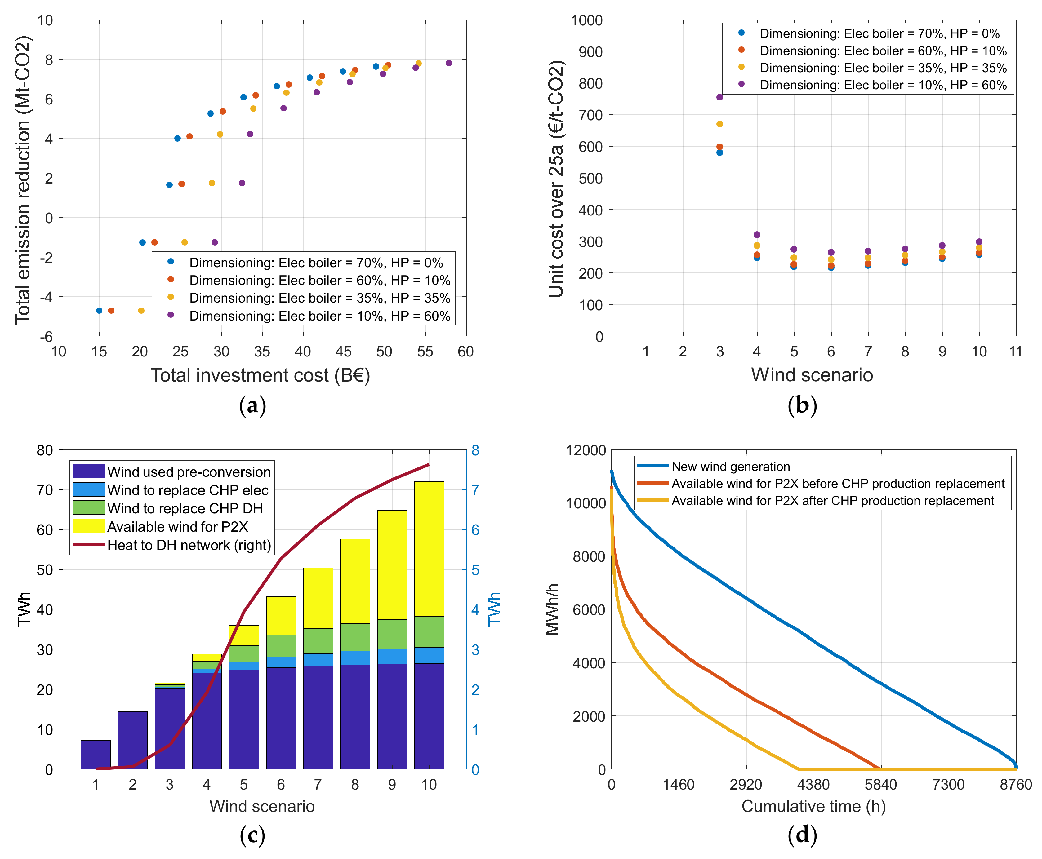
For the P2H conversion four different shares of electric boilers and heat pumps were considered for all wind scenarios, where they were dimensioned to cover the following shares of the peak DH demand of the renovated housing stock.

• Electric boilers 70% and heat pumps 0%.
• Electric boilers 60% and heat pumps 10%.
• Electric boilers 35% and heat pumps 35%.
• Electric boilers 10% and heat pumps 60%.

If a combination of options were used, it was assumed that HPs were utilized before electrode boilers. The replacement of heat from CHP district heat production was assumed possible if there was district heating demand from the renovated buildings during the hour of excess wind power.

In this phase also the supply and demand of electricity were matched if there was still a mismatch after the power system simulation. In situations where the base generation, hydropower, and new wind generation were not enough to satisfy the electricity demand, existing condensing power capacity in Finland, 970 MW in 2017 [4], was assumed to be utilized. If this was still not enough, new combined cycle gas turbine generation (CCGT) was applied to the generation mix to cover the remaining demand. So, by default, import of power was not considered here. This part of the analysis was performed after the optimization of power system operation, including hydropower scheduling, and was done as post-processing with Matlab (v 9.2) and Excel.

This arrangement would lead to minimum carbon emissions with the assumption that the marginal emissions of electricity generation, when the marginal generation is based on combustion, are higher compared to those from district heat generation. In general, these marginal emissions depend on the set of generation available. In Finland, the emissions from district heat are largely based on CHP production, which covers 67% of the total production [26], and thus the emissions must be divided between the heat and power production. In this study these emissions were divided according to the benefit allocation method.

The required investment costs for the new additional wind power capacity, HPs, electric boilers, heat only boilers, and CCGT power plants were calculated and the changes in emissions in electricity and district heating with the added wind capacity scenarios. These were combined to the investment costs of the building renovation scenarios. The total investment costs of different scenarios and their emission reduction potentials were compared to find an efficient combination for reducing carbon emissions. The system setup is illustrated in Scheme 1 below.

2.2. Effects of Building Renovation Measures to District Heat and Electricity Demand

Hirvonen et al. [21,22] previously examined the emission reduction potential and required investment costs in the Finnish single-family houses and apartment buildings with different renovation measures conducted to them. Moreover, they simulated how the different renovation measures affected the energy demand of the buildings. Next, selected renovation scenarios from these studies are described and the effects of them to the electricity and district heating demands of the chosen building stock are presented.

In [21] a base building was defined as a single-family house with 180 m² of heated floor area. The SH building stock was divided into four age categories, SH1 to SH4, according to the Finnish building code in effect at the year of construction. Further, the houses were modeled to use five different heating systems: wood boiler, oil boiler, direct electric heating, district heating, and ground-source heat pump (GSHP). From the oldest age category SH1 to the newest SH4, ground-source heat pumps and district heating increased their relative shares, whereas wood and oil boilers became less common. Direct electric heating was a widely used solution in all age categories. Optimized solutions, comparing emission reductions to life cycle costs of renovations, were calculated for different renovation measures for all the age categories and heating systems. In the optimization it was assumed that houses with direct electric heating and district heating continued to use their current heating system, but other renovation measures were also conducted to them. Whereas houses with existing GSHPs also continued to use them, but no renovation measures were conducted. From buildings with oil boilers, half were expected to switch to GSHPs and half to wood boilers, and buildings with wood boilers half were expected to continue to use wood and half to switch to GSHPs.

This resulted in a great number of Pareto optimal solutions for each building type, from which four (A-D) were highlighted. Scenario A was the highest cost optimal solution, scenario D the least costly one and scenarios B and C were evenly distributed between these. Here only specified scenarios B and D were further investigated. The specific renovation configurations can be found in the original publication, but in addition to the possible change in the main heating system, the measures conducted included renovations, which decreased the overall energy demand of the building, e.g., thermal insulation and additional heat and electricity generation solutions, e.g., solar thermal collectors and solar PV panels.

For this study, the interest was especially on the effect of the renovations on the electricity and district heat demands of the renovated building stock and the corresponding carbon emissions. For estimating these, the hourly simulation data for the energy usage of the reference buildings and scenarios B and D were obtained from the authors of the original study [21]. From this data an hourly district heat and electricity demand for the SH reference and renovated building stock was estimated. This was done by scaling up the hourly district heat demand, electricity demand, and local PV generation data of a single house to cover the total floor are of that particular stock of houses. In addition, excess electricity from local PV generation was assumed to be used in other single-family houses if there was demand at the same hour, but if not, it was assumed to be wasted.

In [22] Hirvonen et al. examined the emission reduction potential in Finnish apartment buildings with different renovation measures. Similarly to single-family houses, simulation was carried out about how the different measures affected the energy demand of the buildings compared to a simulated reference case. Specific optimal renovation scenarios A to D were selected and examined more thoroughly. The scenarios from A to D were defined as the following: A was the lowest emission and highest cost solution, B the average cost solution, C the cost-neutral solution, and D the least-cost solution.

The apartment building stock was divided in to four different age categories AB1 to AB4 according to the building code in effect at the time of construction. A reference building was defined for all age categories, and it was assumed to be heated with district heating. In the simulation three heating systems were defined for the optimized buildings: district heating only, ground-source heat pump with electric backup heating, and exhaust air heat pump (EAHP) with district heating backup. When simulating the optimal renovation solutions each heating system was optimized separately and fixed for each optimization run.

For this study it was assumed that half of all apartment buildings in all age categories kept using district heating. In categories AB1 and AB2 the remaining half was divided equally to utilize GSHPs and EAHPs, each getting a 25% share. Buildings in age categories AB3 and AB4 were already expected to utilize ventilation heat recovery so the EAHP did not provide additional energy savings [22]. Thus, for these categories the remaining half of the building stock was assumed to utilize GSHPs. The specific renovation configurations for each scenario can be found in the original publication. The total floor areas before and after the renovations of the single-family house and apartment building stocks are presented in

Table 1. Total floor areas of the building stocks considered before and after building renovation measures by the building type, age category, and main heating system [21,22].

Heating System	Floor Area Before Renovations (Mm2)
	SH1	SH2	SH3	SH4	AB1	AB2	AB3	AB4
Wood boiler	32.57	18.22	2.69	1.88	-	-	-	-
Oil boiler	13.43	6.07	0.36	0.30	-	-	-	-
Direct electric	16.13	21.42	4.60	3.77	-	-	-	-
Original GSHP	5.36	10.35	5.31	3.82	-	-	-	-
District heating	2.60	8.03	2.69	2.01	46.93	32.68	5.80	8.31
Total	70.09	64.09	15.66	11.79	46.93	32.68	5.80	8.31
	Floor area after renovations (Mm2)
	SH1	SH2	SH3	SH4	AB1	AB2	AB3	AB4
Wood boiler	23.00	12.15	1.52	1.09	-	-	-	-
Oil boiler	0.00	0.00	0.00	0.00	-	-	-	-
Direct electric	16.13	21.42	4.60	3.77	-	-	-	-
Original GSHP	5.36	10.35	5.31	3.82	-	-	-	-
District heating	2.60	8.03	2.69	2.01	23.46	16.34	2.90	4.16
New GSHP	23.00	12.15	1.52	1.09	11.73	8.17	2.90	4.16
New EAHP	-	-	-	-	11.73	8.17	0.00	0.00
Total	70.09	64.09	15.66	11.79	46.93	32.68	5.80	8.31

.

For apartment buildings hourly energy usage data was obtained for scenarios B and C from the authors of the original study [22]. From this data an hourly district heat and electricity demand for the AB reference and renovated building stock was estimated. This was done by scaling up the hourly district heat demand, electricity demand, and local energy generation data of a single apartment building to cover the total floor are of that particular stock of buildings. In addition, excess electricity from local PV was assumed to be used in other apartment buildings if there was demand at the same hour, but if not, it was assumed to be wasted.

To observe the effects of the renovations on the whole housing stock, combinations of the measures conducted to single-family houses and apartment buildings were estimated. This was done by combining the hourly estimations made previously for both building types for different combinations of renovation scenarios.

Based directly on the renovation scenarios of the studies [21,22] four different building renovation scenarios were constructed, where scenario D was the least costly one, C a cost-neutral one, and B a high cost one. The combined scenarios were named cost-wise to include either high-cost measures (B) or low-cost measures (C or D). The four scenarios were:

• SH and AB renovated according to scenario B (SH High and AB High);
• SH renovated according to scenario B and AB according to scenario C (SH High and AB Low);
• SH renovated according to scenario D and AB according to scenario B (SH Low and AB High);
• SH renovated according to scenario D and AB according to scenario C (SH Low and AB Low).

In addition to these scenarios a new scenario was also constructed. In this scenario only the heating systems of the buildings were renovated together with basic refurbishment, which was also performed in all of the other building renovation scenarios. Later this scenario is referred as the “heating only” scenario. Same shares of heating systems after the renovations were used as in the scenarios before. When the heating system was changed in a single-family house the building, which was renovated was expected to have the same energy consumption as the reference building with the same heating system in the same age category. When the heating system was changed in an apartment building from district heating to GSHP or EAHP the total energy demand of the building was assumed to be the same as the reference building with DH in the same age category. For apartment buildings the GSHPs were dimensioned to cover 70% of peak heat demand and the rest was covered with electrical backup heating. EAHPs were dimensioned to cover 20% of the peak demand and backup was covered with DH. For part of the buildings, which continued with their existing heating system, some renovations were performed: district heating was renewed in SH1, SH2, AB1, and AB2 categories and buildings, which continued with wood boilers were expected to renew them with new ones. The investment costs for this scenario were based on the investment costs of the original studies and are presented in

Table 2. Investment costs for renovations conducted in the “heating only” building renovation scenario [21,22].

Heating System	Investment Cost (€/m2)
	SH1	SH2	SH3	SH4	AB1	AB2	AB3	AB4
Wood boiler	106.7	106.7	106.7	106.7	-	-	-	-
Direct electric	78.4	78.4	78.4	78.4	-	-	-	-
Original GSHP	78.4	78.4	78.4	78.4	-	-	-	-
District heating	110.5	93.4	78.4	78.4	110.5	93.4	78.4	78.4
New GSHP	185.3	164.0	153.3	142.6	138.3	126.9	119.7	114.0
New EAHP	-	-	-	-	102.4	113.8	-	-

. For the other renovation scenarios, the investment costs were directly taken from the original publications [21,22].

The effect of different renovation scenarios on the electricity and district heating demands of the building stock compared to the reference building stock are displayed in Figure 1. For electricity demand, the demand of the peak hour increased compared to the reference for all of the renovation scenarios except the “SH High and AB High”, and the annual demand decreased for all except for the “heating only” scenario. For district heating the peak hour demand decreased for all renovation scenarios, as did the annual total demand. In general, the more costly the renovation was the larger the difference was between it and the reference. In

Table 3. The electricity and district heat demands of the renovated building stocks compared to the reference building stock [21,22].

Renovation Scenario	Electricity Demand	DH Demand	Peak Electricity Demand	Peak DH Demand
	TWh/a	TWh/a	MWh/h	MWh/h
Reference	15.4	15.7	5320	5700
SH High and AB High	10.1	3.6	5280	2110
SH High and AB Low	10.4	5.7	5440	2890
SH Low and AB High	13.2	4.4	6400	2350
SH Low and AB Low	13.5	6.5	6560	3120
Heating only	19.8	10.8	8060	4290

the electricity and district heat demands of the renovated building stocks are presented in more detail together with the reference building stock. The electricity and district heat demands of the reference building stock were estimated with data from studies [21,22], where hourly values for the reference single-family houses and apartment buildings were simulated.

2.3. Emission Factors of Different Energy Sources

Reference emissions of the Finnish electricity generation mix were calculated as in [22], which calculated a monthly emission factor for electricity based on historical emission and production data from Finnish Energy for years 2011–2015. Here this is extended to include data from years 2016 and 2017, again based on data from the Finnish Energy [27]. The resulting monthly emission factor is presented in

Table 4. Reference emission factor for electricity before measures to the generation mix were conducted [22].

Month	1.	2.	3.	4.	5.	6.	7.	8.	9.	10.	11.	12.
Emission factor (kg-CO2/MWh)	162.9	159.6	144.0	124.8	118.0	83.3	73.5	99.2	130.0	138.0	130.4	128.6

. The emission factor is greater during periods with a high electricity demand as the share of emission-free generation is lower during those periods. This emission factor was used for calculating the change in the emissions of the SH and AB stock before and after the building renovation scenarios. It was also used for calculating reference emissions for the total electricity demand in Finland for which the emissions from the new generation mixes with different shares of wind power generation were compared to.

Single-family houses that utilized on-site boilers for heat generation used either wood or oil as an energy source. For this study to be comparable to the earlier one for single-family houses [21], wood was considered here to have emissions when used in on-site boilers. The wood fuel was considered to be wood pellets, which have emissions of 403.2 kg-CO₂/MWh [6] and considering the efficiency of the wood boiler, 75%, the emission factor was 538 kg-CO₂/MWh for produced heat. For oil boilers the fuel used was heating fuel oil with low sulphur content. This had emissions of 263 kg-CO₂/MWh [6] and when considering the efficiency of the oil boiler, 81%, the emission factor was 325 kg-CO₂/MWh for produced heat. For both the single-family houses and apartment buildings, which used district heating, a five-year annual national average emission factor of 164 kg-CO₂/MWh from years 2013 to 2017 was used [4]. It considered both the CHP and separate production of district heat and the emissions from CHP production were divided between heat and power by using the benefit allocation method.

When measures were conducted in the energy system the electricity generation mix changed. Thus, new emissions for it needed to be calculated. In the new electricity generation mix, generation forms with carbon emissions were the CHP industry, CHP district heat, existing condensing power, new CCGT generation, and heat only boiler used for priming of heat from the HPs. Except for new CCGT generation and HOBs, emission factors for these generation types were based on five-year average emission factors from 2013 to 2017 for each generation type from [4]. For CHP production these factors divided the emissions between heat and electricity by using the benefit allocation method. The new CCGT power plants were assumed to use natural gas as a fuel with emissions of 199.1 kg-CO₂/MWh [6] and to have an efficiency of 60% [28], resulting in emissions of 332 kg-CO₂/MWh. The HOBs for heat priming were also assumed to use natural gas as a fuel with 94% efficiency [29] resulting in emissions of 212 kg-CO₂/MWh. As the excess wind power production was used to replace electricity and heat generation from CHP district heat production it replaced them by their respective emission factors. Thus, for the replaced heat a different emission factor was used than for the reference DH emission factor, which also considered the separate generation of DH. The emission factors for all generation forms are presented in

Table 5. Emission factors for selected electricity and heat generation methods, considering the efficiency of production [4,6,22,28].

Energy Source	Emission Factor (kg-CO2/MWh)
Reference electricity	74-163
Reference DH	164
On-site wood boiler (heat)	538
On-site oil boiler (heat)	325
CHP industry electricity	119
CHP DH electricity	384
CHP DH heat	177
Existing condensing power	832
New CCGT	332
HOB for heat priming	212

. Notably, these values consider the efficiency of the production, i.e., they are emissions per produced heat or electricity.

2.4. Wind Generation

Statistical modeling of wind power was adopted from study [30]. The method combines probability integral transformation and simulated wind speed time series, allowing the generation of realistic wind power profiles without measurement data. New wind generation was modeled considering the geography and existing fleet of wind turbines in Finland in the beginning of 2016. This existing generation was expanded to include new wind turbines with an average capacity factor of 0.28. The wind power time series was considered in a similar manner as in [23] where more details regarding the power system optimization model can be found. With this methodology wind generation from a new capacity of 1080 MW was simulated over one-year period with 100 simulation runs. Out of the 100 hourly wind profiles generated an average one, where the hourly average is at 50th percentile from all the profiles, was selected for this study. In the simulation of the new Finnish electricity system this average wind power profile was scaled up to obtain various penetration levels of wind generation. Ten different wind generation scenarios were formed from the wind simulation with increments of 2160 MW. The capacities of these wind scenarios are presented in

Table 6. Wind generation capacities used for the ten wind scenarios.

Wind Scenario	1	2	3	4	5	6	7	8	9	10
New wind generation capacity (MW)	2160	4320	6480	8640	10800	12960	15120	17280	19440	21600

.

2.5. Conversion of Excess Wind Generation to Heat

Converting the excess electricity from wind generation to heat to the district heating network, deep geothermal heat pumps, electric boilers, or a combination of these were utilized, together with possible HOBs for priming of heat from the HPs. Here deep geothermal heat pumps refer to a system where a heat pump was coupled to a 2000 m deep borehole heat exchanger. Deep borehole heat exchangers were utilized instead of shallower ones since they can achieve a higher output temperature [31] (p. 287) and require less surface area for the same heat effect, which is beneficial for locations with limited space such as urban areas [19]. The borehole utilized a coaxial pipe and water as a secondary fluid. The operation parameters for the borehole heat exchanger were derived from the simulation results of such BHE in [19] in Finnish geological conditions, which assumed a 40 °C temperature at the depth of 2000 m. An output temperature of 17 °C and inlet temperature of 6 °C were assumed for the borehole, and they were assumed to remain constant over the 25-year period. For obtaining a relatively high output temperature a mass flow rate of 2 kg/s was assumed for the secondary fluid.

The thermal power extracted from the borehole can be calculated with the equation:

$$\Phi = \stackrel{·}{\mathrm{m}}{c}_p\left(T_{\mathrm{out}}-T_{\mathrm{in}}\right)$$

(1)

where $\stackrel{·}{\mathrm{m}}$ is the mass flow rate, c_p the specific heat capacity of water, T_out the outlet temperature, and T_in the inlet temperature of the secondary fluid in the borehole. It is good to note that varying the mass flow rate also affects the outlet temperature of the secondary fluid.

To utilize the geothermal heat in the DH network the temperature of it must be increased, which can be achieved with heat pumps. The COP of the heat pump system can be expressed as [32] (pp. 1–2):

$${\mathrm{COP}}_{\mathrm{System}}= \frac{Q_{\mathrm{cond}}}{W_{\mathrm{comp}}+W_{\mathrm{pump}}}$$

(2)

where Q_cond is the heat output from the condenser, W_comp the work of the compressor, and W_pump the work of the circulating pumps. The theoretical maximum COP, COP_Carnot, can be defined as [32] (pp. 1–2):

$${\mathrm{COP}}_{\mathrm{Carnot}}=\frac{T_{\mathrm{cond}}}{T_{\mathrm{cond}}-T_{\mathrm{evap}}}$$

(3)

where T_cond is the output heat temperature from the condenser and T_evap is the source temperature to the evaporator. To obtain the actual COP of the heat pump inefficiencies must be considered. The COP of the heat pump can be defined thus as [33]:

$${\mathrm{COP}}_{\mathrm{HP}}= {\epsilon }_{\mathrm{Carnot}}{\mathrm{COP}}_{\mathrm{Carnot}}$$

(4)

where ε_Carnot is the Carnot efficiency, which is typically 0.5–0.7 for large heat pump systems [33]. Here a value of 0.6 was used. Further, the COP for the whole system can be expressed as [19]:

$${\mathrm{COP}}_{\mathrm{system}}=\frac{{\mathrm{COP}}_{\mathrm{HP}}{W}_{\mathrm{comp}}}{W_{\mathrm{comp}}+W_{\mathrm{pump}}}=\frac{{\mathrm{COP}}_{\mathrm{HP}}}{1+\frac{W_{\mathrm{pump}}}{W_{\mathrm{comp}}}}$$

(5)

The heat pumps were assumed to be connected to the district heating network on the supply water side. Thus, the DH supply water temperature, T_DH,supply, defined the required output temperature of the heat pump, T_cond, within the temperature limits of the heat pump: they were assumed to have a maximum output temperature of 90 °C. Thus, if the DH supply temperature was higher than this, the temperature of the heat from the heat pump was increased to the required level first by electric boilers and secondly by heat only boilers. In these situations, to calculate how much of the temperature rise was conducted by the HP and how much with boilers a temperature for the return water was required to be estimated. According to [34,35,36] the average return temperature of the DH network varies approximately between 35 and 60 °C in Finland and Sweden. In this study a temperature of 45 °C was assumed. The temperature of the DH supply water depended on the outdoor temperature as followings. If the outdoor temperature, T_outdoor, was higher than 8 °C, T_DH,supply was 70 °C. Otherwise it followed the equation [37] (p. 68):

$$T_{\mathrm{DH},\mathrm{supply}}=115 °\mathrm{C}+\left(T_{\mathrm{dimensioning}}-T_{\mathrm{outdoor}}\right)\frac{45 °\mathrm{C}}{\left(8 °\mathrm{C}-T_{\mathrm{dimensioning}}\right)}$$

(6)

The dimensioning temperature, T_dimensioning, is used when a building’s heating and ventilation systems are designed. Finland is divided into four climate zones, from south to north, with different dimensioning temperatures [38]. When the dimensioning temperature is lower the building is designed according to a colder climate. Here the Zone I dimensioning temperature of -26 °C was used as 41% of the built floor area is located there [39]. The outdoor temperature was based on the outdoor temperature of the weather file Test Reference Year (TRY2012-Vantaa) for climate zones I and II [38], which cover 75% of the built floor area [39]. The weather file was the same as used in studies [21,22] for the building renovation simulations. The outdoor temperature varied between -20.6 and 28.8 °C. The pumping power of the circulation pumps, W_pump, was assumed to be 5 kW. With these parameters the COP for the heat pump system varied between 2.7 and 3.4 depending on the outside temperature and had an average value of 3.1. The heat output power of a single heat pump coupled to a borehole heat exchanger varied between 124 and 139 kW.

According to [40], the ramp up rate of a heat pump is 10% in every 30 s with a warm start-up. In other words, the heat pump could be utilized, when needed, almost instantly when the pump was assumed to be in the standby mode. Standby electricity consumption was not considered here.

Another method to convert the excess wind power to heat was to utilize electric boilers separately, which compared to heat pumps have lower efficiency and lower investment cost. Here electrode boilers were utilized, which have an efficiency of 98% [41]. In the standby mode they have a short start-up time of approximately 30 s and the cold start-up is approximately 5 min [41]. Thus, they could be utilized when needed.

2.6. Investment Costs for Energy System Measures

As one of the objectives for this study was to compare the emission reduction potentials of the building renovations and the energy system measures, an indicator for them was established. It was defined as the investment cost of the measures conducted divided by the achieved emission reductions. The investments were considered to be made for 25 years as in [21,22] and the reduced emissions were assumed to remain constant annually. In the studies [21,22] the investment costs included a 24% value added tax (VAT). For the results from this study to be comparable to the earlier ones a 24% VAT was included in the investment costs made to the energy system. Although, it can be argued that these types of investments would be made by companies and thereby they could subtract the VAT in their taxation as they sell the product from the investments, but in that case the VAT is then paid by the end customer who buys the product. Thus, the VAT was also included in the investment costs conducted to the energy system.

The technical lifetime of wind turbines, heat pumps, CCGT power plants, and natural gas HOBs is 25 years, but for electrode boilers it is 20 years [41]. Thus, the electrode boiler investment needs to be done again in 20 years. For the later investment only the investment for five years was considered, and the residual value of the boiler was assumed to be zero after 20 years of operation.

The investment cost of drilling a 2000 m deep borehole was under a large amount of uncertainty due to a lack of such boreholes drilled in the Nordics. For shallower ground-source heat pump systems the drilling is a significant part of the total investment cost and in [42] Gehlin et al. suggested that the cost increases exponentially with depth. A similar outcome was presented by [43] where a price model for BHEs was derived from a survey submitted for Swedish drillers. Here this price model was extended to the depth of 2000 m and is as follows [43]:

$$C_{\mathrm{I}}=\left(C_1+ C_2{H}^2+C_3\right){\mathrm{N}}_{\mathrm{b}}H+C_0$$

(7)

where C_I is the total investment cost, H is the depth of the borehole, N_b is the number of boreholes, C₁ and C₂ are constants derived from the survey, C₃ includes other costs related to drilling, e.g., casing, and C₀ is the fixed cost of establishing the drill on the drilling site. The values for the previous parameters as in [43] are presented in

Table 7. Parameter values for evaluation of borehole heat exchanger investment cost, without VAT [43,44].

Parameter	Value	Unit
C0	906	€
C1	15.4	€/m
C2	3.29*10-5	€/m3
C3	9.7	€/m

. In the original study the costs were given in SEK, here they were converted to EUR using the 2018 average exchange rate of 10.2583 from [44]. The investment costs for all the measures conducted in the energy system are presented in

Table 8. Unit investment costs for measures conducted in the energy system, with 24% VAT [28,43].

Technology	Investment Cost	Unit
Wind generation	1980	€/kW
New CCGT	1610	€/kW
Heat pump	715	€/kW
Borehole heat exchanger (2000 m)	4240	€/kW
Electrode boiler	95	€/kW
HOB (natural gas)	125	€/kW

.

3. Results

3.1. Carbon Emission Reduction Potential of Measures Conducted in Housing Stock Only

In

Table 9. Emission reduction potential of renovation measures conducted to single-family houses and apartment buildings only. Total investment in billion euros.

Renovation Scenario	Total Investment	Emission Reduction	Unit Cost Over 25 Years
	B€	Mt-CO2/a	€/t-CO2
SH High and AB High	85.8	8.88	387
SH High and AB Low	73.0	8.49	344
SH Low and AB High	59.2	7.29	325
SH Low and AB Low	46.4	6.89	269
Heating only	27.9	3.54	316

the emission reduction potential of the measures conducted to single-family houses and apartment buildings are presented. These differ from the results presented by the previous studies [21,22] for a couple of reasons: here the same emission factor for district heating was used for both building types, the reference electricity emission factor was extended to include data from years 2016 and 2017, the efficiencies of the wood and oil boilers used were 75% and 81% respectively, and the apartment building stock was divided to utilize a different heating system as defined in Section 2.2. In addition, here the renovation scenarios were combined to include the buildings stocks of both building types, which was not done in studies [21,22] as they were separate.

For the renovation scenarios, which were directly based on the renovation scenarios in studies [21,22], the investment costs increased together with the reduced emissions. The scenario constructed here but based on data of the previous studies, “heating only”, was the least costly one and the one with lowest total emission reduction. In the “heating only” scenario only the heating systems were renovated, as described in Section 2.2, but no other energy saving measures were conducted to the buildings. When comparing the unit costs of emission reductions, i.e., the total investment costs and emission reductions over 25 years, the least costly one was the scenario where single-family houses were renovated according to a low-cost scenario (D) and apartment buildings according to a low-cost scenario (C). The “heating only” scenario was the second lowest in terms of unit cost. Hence, the additional renovation measures in scenario “SH Low and AB Low” increased the total investment cost compared to the “heating only” scenario but at the same time increased the reduced emissions more in relation.

3.2. Measures in the Energy System with Building Renovation Scenario “SH High and AB High”

Figure 2 presents the results of energy system measures when buildings were renovated according to scenario “SH High and AB High”. This was the high cost and high emission reduction renovation scenario for the buildings. In Figure 2a the total investment costs and emission reductions for the ten wind scenarios with four different options for heat conversion of excess wind are presented, when emission reductions were calculated for the total electricity demand in Finland and the DH demand of the renovated SH and AB stock. Notably the emissions increased with the lowest increase in wind generation capacity by 1.6 Mt of CO₂ for all the different dimensioning options of electrode boilers and HPs coupled to 2000 m deep borehole heat exchangers. This is since no import of electricity was considered here and thus, especially for the lowest increase of wind generation, the existing condensing power was utilized extensively together with new CCGT generation. The effect of having the option of electricity import on the results is later examined in Section 3.9. For the later wind capacity increases the generation increased such that even though existing condensing and new CCGT generation were required the total emissions decreased. In addition, the highest emission reduction for all wind scenarios was reached with the heat conversion option where HPs were dimensioned to cover 60% of the peak DH demand and electrode boilers to 10%. Moreover, the emissions reductions reached the level of 5.2 Mt of CO₂ with the highest increase in wind capacity. Figure 2b displays the unit cost (€/t-CO₂) of emission reductions over 25 years, for scenarios that reduced emissions, when the emission reductions were expected to remain constant annually. It shows that the lowest unit costs of emission reductions were reached with wind scenario 3 with 6480 MW of the new wind capacity. Additionally, the lowest unit cost, 187 €/t-CO₂, was attained when only electrode boilers were utilized for the P2H conversion.

In Figure 2c the least-cost heat conversion method for all wind scenarios, boiler 70% and HP 0%, was examined in more detail. In dark blue the amount of new wind power used annually in the electricity mix before any CHP replacement was applied is shown. The figure shows that the amount of new wind generation pre-conversion did not increase significantly after wind scenario 3 where already an annual consumption of 16.5 TWh was reached. For wind scenario 10 this consumption increased to 18.0 TWh. As excess wind generation was converted to heat to replace heat production from CHP district heat, also electricity from the CHP production needed to be replaced according to the power-to-heat ratio of 0.52. In Figure 2c the new wind generation, which was used to replace electricity from the CHP district heat generation is displayed in light blue and wind used to replace heat production from the CHP district heat production in green. As seen from the figure the amount of wind used in the conversion increased as the wind generation capacity increased and there was more excess wind available for the conversion. Additionally, for the lowest unit cost scenario, wind scenario 3, the replacement of CHP production increased the utilization of the wind power from 16.5 to 18.0 TWh annually. In wind scenarios with a high amount of wind generation the energy sink of the district heating system was not enough to absorb all the excess wind generation. Thus, in yellow the amount of new wind generation that was available for other power-to-X (P2X) applications after the CHP replacement is shown. In addition, in Figure 2c the annual amount of heat supplied to the DH network converted from the excess wind is displayed. It reached the amount of 2.9 TWh for wind scenario 10, and for the lowest unit cost wind scenario, scenario 3, it was 0.9 TWh, as the total DH demand of the renovated buildings was 3.6 TWh. For the supplied heat, the right axis was used.

In Figure 2d load duration curves of new wind generation and excess wind generation before and after the replacement of electricity and heat from CHP district heat production are presented for the lowest unit cost scenario, wind scenario 3 with boilers dimensioned to 70% of peak DH demand, when buildings were renovated according to building renovation scenario “SH High and AB High”. It shows that majority of the new wind generation was utilized in the electricity mix, and the CHP replacement increased its utilization and that the remaining excess wind contained high peak power values.

In

Table 10. Lowest unit cost of emission reductions for energy system measures for different P2H options when buildings were renovated according to scenario “SH High and AB High”. Wind power used in the electricity mix includes direct utilization and electricity replaced from CHP district heat production. Heat from the electrode boiler includes both priming of heat from HPs and separate production.

	Elec Boiler 70% HP 0%	Elec Boiler 60% HP 10%	Elec Boiler 35% HP 35%	Elec Boiler 10% HP 60%	Unit
New wind capacity (scenario)	6480 (3)	6480 (3)	6480 (3)	6480 (3)	MW
HP capacity	0	211	740	1268	MW
Elec boiler capacity	1480	1268	740	211	MW
Heat boiler capacity	0	90	338	475	MW
New wind generation	21.60	21.60	21.60	21.60	TWh/a
Wind used in electricity mix	17.02	17.05	17.08	17.09	TWh/a
Wind converted to heat	0.94	0.69	0.43	0.38	TWh/a
New heat to DH network	0.92	0.98	1.05	1.06	TWh/a
Of which HP; elec B; heat B	0.0; 0.92; 0.0	0.45; 0.53; 0.001	0.96; 0.09; 0.007	1.03; 0.01; 0.01	TWh/a
Remaining excess wind	3.64	3.86	4.01	4.13	TWh/a
Unit cost	187	194	214	234	€/t-CO2

the utilization of the new wind generation is displayed in more detail for the lowest unit cost wind scenarios for all the P2H options. Electrode boilers were first used for priming the heat from HPs if necessary and then separately for converting excess wind to heat to the DH network. The heat boilers presented in Table 10 are the ones used for only priming the heat from HPs when necessary if electrode boilers were not possible to use due to either a lack in capacity or available excess wind. As heat pump capacity was increased also more heat boiler capacity for priming was required. Although simultaneously with increased HP capacity the electrode boiler capacity was decreased the main reason for increased heat boiler usage was the increased HP capacity; even though electrode boilers would have been dimensioned to 60% of peak DH demand when HPs were dimensioned to 60% the required heat boiler capacity would have been the same as when electrode boilers were dimensioned to 10%. In that case the heat from heat boilers would have however decreased slightly from 0.0122 to 0.0095 TWh. In addition, in Table 10 the amount of new wind generation used in the electricity mix, including wind used to replace electricity from CHP district heat generation, wind converted to heat, and new heat supplied to the DH network are presented. When HPs were used more extensively than electrode boilers the amount of wind used for heat conversion decreased but supplied heat to the DH network increased, as HPs had a higher conversion efficiency compared to electrode boilers. Additionally, the remaining excess wind generation after the CHP replacement is presented, as is the unit cost of emission reduction for the different solutions.

3.3. Measures in the Energy System with the Building Renovation Scenario “SH High and AB Low”

Building renovation scenario “SH High and AB Low” was a scenario where SHs were renovated according to a high cost scenario and ABs according to a lower cost scenario. Here the results of energy system measures are presented when the buildings were renovated according to these measures. Figure 3 displays the results in a similar fashion as Figure 2. Figure 3a shows the total emission reduction and investment costs for the wind scenarios with different options for heat conversion of excess wind production. For the lowest increase in wind generation capacity the emissions increased approximately by 1.8 Mt of CO₂ but for the other wind scenarios the emissions decreased. This is due to the lack of import considered here and thus the existing condensing power and new CCGT generation were used extensively, especially for the first wind scenario. Additionally, the highest emission reduction, 5.9 Mt-CO₂, was attained with wind scenario 10 when HPs were dimensioned to 60% and electrode boilers to 10% of the peak DH demand of the renovated buildings. Figure 3b displays the unit costs of the emission reductions for the wind scenarios, which reduced emissions. For all the wind scenarios the lowest unit cost of emission reductions was reached when only electrode boilers were utilized, dimensioned to cover 70% of the peak DH demand. Moreover, the lowest unit cost, 181 €/t-CO₂, was reached with wind scenario 3 with a new wind generation capacity of 6480 MW.

In Figure 3c the least-cost heat conversion option, boiler 70% and HP 0%, was examined in more detail. For wind scenarios 1 and 2 the wind used for the CHP replacement was low but as wind generation capacity was increased also the wind used for CHP replacement increased from 2.0 TWh in scenario 3 to 7.2 TWh in scenario 9. Notably the wind used for the CHP replacement and the new heat supplied to the DH network decreased in scenario 10 compared to scenario 9. This is due to the order of the measures conducted. First the new wind generation was utilized in the electricity mix as much as possible with hydropower used to mitigate the difference between the supply and demand. This affected how much of the excess wind was hourly available and how well it matched with the DH demand of the renovated buildings. After this the excess wind was utilized for replacing the CHP production. Therefore, the amount of new wind utilized in the electricity mix before any CHP replacement increased but the total utilization after it decreased by 0.03 TWh. However, the total emission reduction increased in wind scenario 10 but the difference was only 0.01 Mt-CO₂ compared to wind scenario 9. For wind scenario 3, with heat conversion conducted with an electrode boiler only, the total utilization of new wind generation was 18.8 TWh, which increased to 25.3 TWh for wind scenario 9. Notably, as the DH demand of the buildings was higher, as the apartment buildings were renovated according to a lower cost scenario, the amount of new heat supplied to the DH network was higher compared to the earlier building renovation scenario “SH High and AB High”.

In Figure 3d load duration curves of new wind generation and excess wind generation before and after the replacement of CHP electricity and heat production are presented for the lowest unit cost scenario, wind scenario 3 with electrode boilers dimensioned to 70% of peak DH demand, when buildings were renovated according to building renovation scenario “SH High and AB Low”. Majority of the new wind generation was utilized directly in the electricity mix, and the CHP replacement increased its utilization and that the remaining excess wind contained high peak power values.

In

Table 11. Lowest unit cost of emission reductions for energy system measures for different P2H options when buildings were renovated according to scenario “SH High and AB Low”. Wind used in the electricity mix includes direct utilization and electricity replaced from CHP district heat production. Heat from electrode boilers includes both priming of heat from HPs and separate production.

	Elec Boiler 70% HP 0%	Elec Boiler 60% HP 10%	Elec Boiler 35% HP 35%	Elec Boiler 10% HP 60%	Unit
New wind capacity (scenario)	6480 (3)	6480 (3)	6480 (3)	6480 (3)	MW
HP capacity	0	289	1010	1731	MW
Elec boiler capacity	2020	1731	1010	289	MW
Heat boiler capacity	0	84	476	634	MW
New wind generation	21.60	21.60	21.60	21.60	TWh/a
Wind used in electricity mix	17.41	17.48	17.56	17.57	TWh/a
Wind converted to heat	1.36	1.08	0.67	0.57	TWh/a
New heat to DH network	1.33	1.46	1.62	1.64	TWh/a
Of which HP; elec B; heat B	0.0; 1.33; 0.0	0.61; 0.85; 0.001	1.46; 0.15; 0.01	1.61; 0.01; 0.02	TWh/a
Remaining excess wind	2.83	3.04	3.37	3.45	TWh/a
Unit cost	181	189	213	239	€/t-CO2

the utilization of the new wind generation is displayed in more detail for the lowest unit cost wind scenarios for all the P2H options in the same manner as in Table 10. Electrode boilers were first utilized for priming the heat from HPs if necessary and then separately for heat production from excess wind generation. Heat boilers were utilized only for priming the heat from HPs if electrode boilers were not possible to be used. Wind used in the electricity mix includes both direct utilization and electricity replaced from the CHP district heat production. Heat from electrode boilers includes both priming of heat from HPs and separate production. As HPs were used more extensively the heat supplied to the DH network increased. Similarly, the electricity used in the electricity mix increased as more CHP district heat electricity production was possible to be replaced. Additionally, the remaining excess wind generation increased as heat pumps had a higher efficiency compared to electrode boilers. Moreover, the unit cost of emission reductions increased as HPs were used more widely.

3.4. Measures in the Energy System with Building Renovation Scenario “SH Low and AB High”

Building renovation scenario “SH Low and AB High” was a scenario where SHs were renovated according to a low-cost scenario and ABs according to a higher cost scenario. Here the results of energy system measures are presented when buildings were renovated according to this scenario. Figure 4 presents the results in a similar fashion as Figure 2. In Figure 4a the total emission reductions and investment costs are presented for the 10 wind scenarios with four options for the heat conversion of excess wind generation. As previously the lowest increase of wind power generation increased the emissions, for this scenario 2.6 Mt of CO₂, as a large amount of existing condensing power and new CCGT generation were needed. The largest annual emission reduction of 5.6 Mt-CO₂ was achieved with wind scenario 10 utilizing heat pumps dimensioned to 60% and electrode boilers to 10% of the peak DH demand of the renovated buildings for the heat conversion, but the difference to other conversion options was small.

Figure 4b shows the unit costs of the emission reductions for wind scenarios, which reduced emissions. Wind scenario 2 resulted in high unit costs but for the rest of the wind scenarios the unit costs were all below 400 €/t-CO₂. Again, the lowest unit costs were achieved when utilizing only electrode boilers for the heat conversion, and the lowest of unit cost of 204 €/t-CO₂ with wind scenario 4 with a new wind generation capacity of 8640 MW.

Figure 4c shows the utilization of new wind power generation for the lowest unit cost heat conversion option; electrode boiler capacity dimensioned to cover 70% of the peak DH demand of the renovated buildings. After wind scenario 3 the increase in the utilization of new wind generation, before CHP production replacement was conducted, slowed down as it increased from 18.7 TWh in wind scenario 3 to 20.7 TWh in scenario 10. After wind scenario 3 the amount of excess wind generation, which was used to replace heat from the CHP district heat production, and the corresponding electricity generation increased, and for wind scenario 4 2.9 TWh of the new wind generation was utilized for this replacement. In total, the utilization of new wind generation increased from 22.3 to 26.0 TWh from wind scenario 4 to scenario 10. Notably, the heat supplied to the district heat network did not increase after wind scenario 8 due to the order of the measures conducted as explained in Section 3.3, but here the total utilization of wind generation still increased. In addition, for the lowest unit cost wind scenario, scenario 4, the excess wind generation available for other P2X applications was 6.5 TWh after the replacement of CHP was considered.

In Figure 4d load duration curves of new wind generation and excess wind generation before and after the replacement of CHP electricity and heat production are presented for the lowest unit cost scenario, wind scenario 4 with electrode boilers dimensioned to 70% of peak DH demand, when buildings were renovated according to the building renovation scenario “SH Low and AB High”. It shows that majority of the new wind generation was utilized directly in the electricity mix, and the heat conversion increased its utilization and that the remaining excess wind contains high peak power values.

In

Table 12. Lowest unit cost of emission reductions for energy system measures for different P2H options when buildings were renovated according to scenario “SH Low and AB High”. Wind used in the electricity mix includes direct utilization and electricity replaced from CHP district heat production. Heat from electrode boilers includes both priming of heat from HPs and separate production.

	Elec Boiler 70% HP 0%	Elec Boiler 60% HP 10%	Elec Boiler 35% HP 35%	Elec Boiler 10% HP 60%	Unit
New wind capacity (scenario)	8640 (4)	8640 (4)	8640 (4)	8640 (4)	MW
HP capacity	0	235	822	1409	MW
Elec boiler capacity	1643	1409	822	235	MW
Heat boiler capacity	0	54	291	438	MW
New wind generation	28.80	28.80	28.80	28.80	TWh/a
Wind used in electricity mix	20.40	20.44	20.48	20.49	TWh/a
Wind converted to heat	1.90	1.39	0.84	0.73	TWh/a
New heat to DH network	1.86	1.93	2.00	2.02	TWh/a
Of which HP; elec B; heat B	0.0; 1.86; 0.0	0.85; 1.09; 0.0003	1.80; 0.20; 0.003	1.97; 0.03; 0.03	TWh/a
Remaining excess wind	6.50	6.96	7.48	7.58	TWh/a
Unit cost	204	210	228	247	€/t-CO2

the utilization of the new wind generation is displayed in more detail for the lowest unit cost wind scenarios for all the P2H options in the same manner as in Table 10. Electrode boilers were first utilized for priming the heat from HPs if necessary and then separately for heat production from excess wind generation. Heat boilers were utilized only for priming the heat from HPs if electrode boilers were not possible to be used. Wind used in the electricity mix includes both direct utilization and electricity replaced from CHP district heat production. Heat from electrode boilers includes both priming of heat from HPs and separate production. As HPs were used more extensively the heat supplied to the DH network increased. Similarly, the electricity used in the electricity mix increased as more CHP district heat electricity production was possible to be replaced. Additionally, the remaining excess wind generation increased as heat pumps had a higher efficiency compared to electrode boilers. Moreover, the unit cost of emission reductions increased as HPs were used more widely.

3.5. Measures in the Energy System with the Building Renovation Scenario “SH Low and AB Low”

Here the results from the energy system measures are presented when the buildings were renovated according to the buildings renovation scenario “SH Low and AB Low”. In this building renovation scenario both the single-family houses and apartment buildings were renovated according to a lower cost scenario. Figure 5 presents the results in a similar fashion as Figure 2. In Figure 5a the total emission reductions and investment costs are presented for the 10 wind scenarios with four options for the heat conversion of excess wind generation. For the first wind scenario the emissions increased by 2.7 Mt of CO₂ but as more wind generation was added the emissions decreased as less existing condensing power and new CCGT generation were required. The largest emission reduction, 6.3 Mt-CO₂, was achieved with wind scenario 10 and HPs dimensioned to 60% and electrode boilers to 10% of the peak DH demand of the renovated buildings.

Figure 5b presents the unit costs of the emission reductions over a 25-year period for wind scenarios that reduced emissions. Wind scenario 2 resulted in high unit costs as the emission reduction was relatively low since existing condensing power and new CCGT generation were still required extensively. However, the need of these decreased as wind capacity was further increased, and the emission reductions increased significantly and thus the corresponding unit costs became substantially lower. The lowest unit costs were achieved when only electrode boilers were utilized for the P2H conversion. Moreover, the lowest unit cost, 198 €/t-CO₂, of emission reductions was achieved with added wind capacity of 8640 MW in wind scenario 4.

Figure 5c examines in more detail the utilization of the new wind generation when the heat conversion was done by utilizing only electrode boilers dimensioned to cover 70% of the peak DH demand of the renovated buildings. For wind scenarios 3 and above, a notable part of the excess wind production was used to replace heat and electricity from CHP district heat production, which increased the utilization of new wind generation, which was, without the CHP replacement, limited to 21.0 TWh in wind scenario 10. In wind scenario 4 when excess wind was used for the CHP production replacement it increased the utilization of the new wind generation from 19.7 to 23.3 TWh. For wind scenario 10 the corresponding values were 21.0 TWh and 28.6 TWh respectively. New heat supplied to the DH network with boiler utilization only is displayed in Figure 5c in the right axis, and notably it decreased in wind scenarios 8 and 10 compared to scenarios 7 and 9, respectively. This is due to the order of measures conducted: first the new wind generation was utilized in the electricity system as much as possible and after this it was used to replace CHP district heat and electricity production as explained in Section 3.3. Nevertheless, the total utilization of new wind generation increased through wind scenarios 7–10.

In Figure 5d load duration curves of new wind generation and excess wind generation before and after the replacement of CHP electricity and heat production are presented for the lowest unit cost scenario, wind scenario 4 with a boiler dimensioned to 70% of the peak DH demand, when buildings were renovated according to building renovation scenario “SH Low and AB Low”. It shows that majority of the new wind generation was utilized in the electricity mix, and the heat conversion increased its utilization and that the remaining excess wind contained high peak power values.

In

Table 13. Lowest unit cost of emission reductions for energy system measures for different P2H options when buildings were renovated according to scenario “SH Low and AB Low”. Wind used in the electricity mix includes direct utilization and electricity replaced from CHP district heat production. Heat from electrode boilers includes both priming of heat from HPs and separate production.

	Elec Boiler 70% HP 0%	Elec Boiler 60% HP 10%	Elec Boiler 35% HP 35%	Elec Boiler 10% HP 60%	Unit
New wind capacity (scenario)	8640 (4)	8640 (4)	8640 (4)	8640 (4)	MW
HP capacity	0	312	1091	1869	MW
Elec boiler capacity	2181	1869	1091	312	MW
Heat boiler capacity	0	76	425	710	MW
New wind generation	28.80	28.80	28.80	28.80	TWh/a
Wind used in electricity mix	20.89	20.97	21.06	21.08	TWh/a
Wind converted to heat	2.41	1.89	1.15	0.97	TWh/a
New heat to DH network	2.36	2.51	2.70	2.73	TWh/a
Of which HP; elec B; heat B	0.0; 2.36; 0.0	0.99; 1.52; 0.01	2.38; 0.31; 0.04	2.67; 0.04; 0.03	TWh/a
Remaining excess wind	5.50	5.94	6.58	6.75	TWh/a
Unit cost	198	205	226	249	€/t-CO2

the utilization of the new wind generation is displayed in more detail for the lowest unit cost wind scenarios for all the P2H options in the same manner as in Table 10. Electrode boilers were first utilized for priming the heat from HPs if necessary and then separately for heat production from excess wind generation. Heat boilers were utilized only for priming the heat from HPs if electrode boilers were not possible to be used. Wind used in electricity mix includes both direct utilization and electricity replaced from CHP district heat production. Heat from electrode boilers includes both priming of heat from HPs and separate production. As HPs were used more extensively the heat supplied to the DH network increased. Similarly, the electricity used in the electricity mix increased as more CHP district heat electricity production was possible to be replaced. Additionally, the remaining excess wind generation increased as heat pumps had a higher efficiency compared to electrode boilers. Moreover, the unit cost of emission reductions increased as HPs were used more widely.

3.6. Measures in the Energy System with the Building Renovation Scenario “Heating Only”

Here results from the energy system measures are presented when the buildings were renovated according to the building renovation scenario “Heating only”. In this building renovation scenario only the heating systems were renovated together with a basic refurbishment as explained in Section 2.2. In addition, this was the only building renovation scenario in which the annual electricity demand increased, and the annual DH demand remained relatively high compared to the other building renovation scenarios.

Figure 6 presents the results in a similar fashion as Figure 2. In Figure 6a the total emission reductions and investment costs are presented for the 10 wind scenarios with four options for the heat conversion of excess wind generation. Differently from the previous building renovation and wind scenarios, here the emissions increased for two of the first additions of wind generation. For the first wind scenario they increased by 4.7 Mt of CO₂ for all the power-to-heat conversion options. From wind scenario 3 onwards the emissions decreased as the new wind generation became higher and less of the existing condensing power and new CCGT generation were required. The largest emission reduction of 7.8 Mt-CO₂ was achieved with wind scenario 10 when utilizing only heat pumps dimensioned to 60% and electrode boilers to 10% of the peak DH demand of the renovated buildings.

Figure 6b presents the unit cost of the emission reductions over a 25-year period for wind scenarios that reduced emissions. The lowest unit costs were achieved when utilizing only electrode boilers for the P2H conversion. Moreover, the lowest unit cost, 216 €/t-CO₂, of emission reductions was achieved with added wind capacity of 12960 MW in wind scenario 6.

Figure 6c examines more thoroughly the wind scenarios with only electrode boilers utilized for the P2H conversion. As the electricity demand was higher compared to the other building renovation scenarios also the amount of wind generation possible to be utilized in the electricity mix was greater. Additionally, the DH demand from the buildings was higher and thus there was more potential for the P2H conversion of excess wind production. The replacement of heat and electricity from CHP district heat production increased the utilization of the new wind generation significantly: for wind scenario 3 from 20.3 to 21.2 TWh and for wind scenario 10 from 26.5 to 38.2 TWh annually. For the lowest unit cost scenario, wind scenario 6, these values were 25.4 TWh and 33.5 TWh respectively. In addition, the new heat supplied to the DH network reached 7.6 TWh with wind scenario 10 in Figure 6c using the right axis, as the total DH demand from the renovated buildings was 10.8 TWh annually.

In Figure 6d load duration curves of new wind generation and excess wind generation before and after the replacement of CHP electricity and heat production are presented for the lowest unit cost scenario, wind scenario 6 with electrode boilers dimensioned to 70% of the peak DH demand, when buildings were renovated according to building renovation scenario “heating only”. It shows that majority of the new wind generation was utilized in the electricity mix, and the CHP replacement increased its utilization and that the remaining excess wind contained high peak power values.

In

Table 14. Lowest unit cost of emission reductions for energy system measures for different P2H options when buildings were renovated according to scenario “heating only”. Wind used in electricity mix includes direct utilization and electricity replaced from CHP district heat production. Heat from electrode boilers includes both priming of heat from HPs and separate production.

	Elec Boiler 70% HP 0%	Elec Boiler 60% HP 10%	Elec Boiler 35% HP 35%	Elec Boiler 10% HP 60%	Unit
New wind capacity (scenario)	12960 (6)	12960 (6)	12960 (6)	12960 (6)	MW
HP capacity	0	429	1503	2576	MW
Elec boiler capacity	3006	2576	1503	429	MW
Heat boiler capacity	0	73	652	884	MW
New wind generation	43.20	43.20	43.20	43.20	TWh/a
Wind used in electricity mix	28.12	28.26	28.44	28.49	TWh/a
Wind converted to heat	5.37	4.23	2.62	2.07	TWh/a
New heat to DH network	5.27	5.54	5.89	5.98	TWh/a
Of which HP; elec B; heat B	0.0; 5.27; 0.0	2.07; 3.47; 0.001	5.00; 0.88; 0.01	5.85; 0.07; 0.06	TWh/a
Remaining excess wind	9.70	10.71	12.14	12.64	TWh/a
Unit cost	216	222	241	264	€/t-CO2

the utilization of the new wind generation is displayed in more detail for the lowest unit cost wind scenarios for all the P2H options in the same manner as in Table 10. Electrode boilers were first utilized for priming the heat from HPs if necessary and then separately for heat production from excess wind generation. Heat boilers were utilized only for priming the heat from HPs if electrode boilers were not possible to be used. Wind used in the electricity mix includes both direct utilization and electricity replaced from CHP district heat production. Heat from electrode boilers includes both priming of heat from HPs and separate production. As HPs were used more extensively the heat supplied to the DH network increased. Similarly, the electricity used in the electricity mix increased as more CHP district heat electricity production was possible to be replaced. Additionally, the remaining excess wind generation increased as heat pumps had a higher efficiency compared to electrode boilers. Moreover, the unit cost of emission reductions increased as HPs were used more widely.

3.7. Energy System Measures with the Lowest Unit Costs

In

Table 15. The investment costs and emission reductions of the lowest unit cost energy system measures for each of the building renovation scenarios.

	SH High and AB High	SH High and AB Low	SH Low and AB High	SH Low and AB Low	Heating Only	Unit
Wind capacity	6480	6480	8640	8640	12960	MW
Wind investment	12.83	12.83	17.11	17.11	25.66	B€
Elec boiler investment	0.14	0.19	0.16	0.21	0.29	B€
CCGT investment	3.34	3.41	4.13	4.41	6.72	B€
Emission reduction electricity	3.33	3.40	3.88	3.97	5.13	Mt-CO2/a
Emission reduction DH	0.16	0.24	0.33	0.42	0.93	Mt-CO2/a
Unit cost	187	181	204	198	216	€/t-CO2
Unit cost, no P2H	206	207	2281	2331	2981	€/t-CO2

1. The unit cost was not achieved with the same wind scenario, as with the P2H option and thus the investment costs and emission reductions in the table do not correspond to this unit cost.

the energy system measures with the lowest unit cost of emission reductions for each of the building renovation scenarios are presented. Here only the energy system measures were considered, although it is good to note that when the energy system measures were applied always one of the building renovation scenarios was expected to be conducted, which affected the electricity and DH demands. For all scenarios presented in Table 15 only electrode boilers were utilized for the P2H conversion. The lowest unit cost of energy system measures was achieved when buildings were renovated according to scenario “SH High and AB Low”, and for the building renovation scenario “SH High and AB High” the unit costs were only slightly higher. These were the renovation scenarios that reduced the overall electricity consumption the most and had the lowest peak electricity demands. For all scenarios, the wind investment cost was the most significant one, but also the investments for new CCGT generation were considerable. The CCGT generation was utilized as a last resort to cover the difference between the electricity supply and demand, and the total annual generation was below 1 TWh for all the scenarios in Table 15. It was utilized for peak power production, which required a high capacity due to the variability of the wind generation and thus also the required investments were high. For all the scenarios in Table 15 a majority of the emission reductions were obtained from the electricity consumption where the reductions were calculated for the total electricity consumption in Finland. The reductions from DH production were higher when the demand from the renovated buildings were higher and for scenarios with larger added wind capacity.

Moreover, in the last row the unit costs of emission reductions are shown in the case that the excess wind generation would not have been used to replace heat and electricity from CHP district heat production, but the wind and CCGT investments would have been conducted as before. Notably for all the renovation scenarios the unit costs increased if the P2H option was not utilized. This further denotes that the additional investments made for converting the excess wind to heat were a cost-efficient manner to increase the emission reductions. Note, that for the first two building renovation scenarios the lowest unit cost was achieved with the same wind scenario as with the P2H option available but for the rest of the renovation scenarios it was not. Thus, the investment costs and emission reductions in the table do not correspond to these unit costs. For them, the lowest unit cost was achieved with a lower increase in wind generation capacity.

3.8. Combined Emission Reduction Potential of Building Renovations and Energy System Measures

The energy system measures, added wind power, power-to-heat conversion, and new CCGT generation were always applied to an energy mix where one of the building renovation scenarios was already expected to be conducted. Thus, it is important to examine the combined emission reduction potential of the building renovations and the energy system measures.

Table 16. The total investment costs and the corresponding emission reductions for the building renovation scenarios, lowest unit cost energy system measures, and the combined results of these.

Building Renovation Scenario	Building Renovations		Energy System Measures		Combined Results
	Total Investment	Total Emission Reduction	Total Investment	Total Emission Reduction	Total Investment	Total Emission Reduction	Emission Reduction Compared to Reference	Unit Cost Over 25 Years
	B€	Mt-CO2/a	B€	Mt-CO2/a	B€	Mt-CO2/a	%	€/t-CO2
SH High and AB High	85.8	8.88	16.3	3.49	102.2	12.37	60	331
SH High and AB Low	73.0	8.49	16.4	3.64	89.4	12.12	59	295
SH Low and AB High	59.2	7.29	21.4	4.20	80.6	11.49	56	281
SH Low and AB Low	46.4	6.89	21.7	4.39	68.1	11.29	55	241
Heating only	27.9	3.54	32.7	6.06	60.6	9.60	47	253

presents the combined emission reduction potentials together with the corresponding investment costs. The energy system measures chosen were the ones with the lowest unit cost of emission reductions with each of the building renovations, i.e., the ones presented in Table 15.

For the building renovations a larger emission reduction was achieved as the investments for the renovations were increased. With the lowest unit cost energy system measures, a larger emission reduction was achieved the less the buildings were renovated. Moreover, the higher the emission reduction with the energy system measures the higher was also the required investment cost. Except for the “heating only” scenario, the investments conducted to the buildings were greater than the investments conducted to the energy system. Additionally, the reduced emission reductions achieved were greater from the buildings, again except for the “heating only” scenario. However, if the unit costs of emission reductions are compared from Table 9 and Table 15 the energy system measures were less expensive compared to the renovation measures conducted to the buildings.

The lowest combined unit cost of emission reductions, 241 €/t-CO₂, was achieved when the buildings were renovated according to the building renovation scenario “SH Low and AB Low” and energy system measures conducted as described in Section 3.5. for the lowest unit cost wind scenario: added wind capacity was 8640 MW and only electrode boilers were utilized for the P2H conversion to replace heat from CHP district heat production. For this combination, the reduced emissions were 11.29 Mt-CO₂ annually. The highest combined reduction, 12.37 Mt-CO₂, was attained with a building renovation scenario “SH High and AB High” together with its lowest unit cost energy system measures, but for this solution the investment cost increased significantly to 102.2 billion euros, compared to 68.1 billion euros for the lowest unit cost solution. If the emissions for electricity consumption in Finland and for the reference housing stock were calculated with the reference emission factors from Table 5, which considered on-site wood boilers used for heating in houses to have emissions, the annual emissions would be 20.6 Mt-CO₂. Compared to these calculated reference emissions, the combined measures presented in Table 16 could result in emission reductions of 47%–60%. With the lowest unit cost solution, the achieved emission reduction could be 55% compared to the reference emissions.

3.9. Considering Import of Electricity

For the previous results import of electricity was not considered. In 2018 Finland imported 23% of the total electricity consumption [4]. Thus, the effect of imported power was examined here briefly. For the calculations everything else remained as before, but before using new CCGT generation to cover the remaining difference between electricity supply and demand, import was used. This means that existing condensing power was still assumed to be used before the import. Import capacity in 2017 was 5200 MW [45], which was considered as the maximum value here. The shares of import from Sweden, Russia, Estonia, and Norway are 5-year averages from [20] and presented in

Table 17. Emission factors for imported electricity and shares of imported electricity to Finland by country [20,46,47].

Country	Share of Import	Emission Factor
	%	kg-CO2/MWh
Sweden	74.7	13
Russia	22.7	517
Estonia	1.9	819
Norway	0.7	9
Total	100.0	143

. The emission factors for the imported electricity were considered as the national average emission factors of electricity for each country. For Sweden and Estonia, the national average emission factors in 2016 were obtained from [46]. For Norway and Russia, the emission factors are from [47] and based on data from 2015. The emission factors for the imported electricity from different countries are presented in Table 17.

In

Table 18. The investment costs and emissions reductions of the lowest unit cost energy system measures for each of the building renovation scenarios when considering the import of electricity.

	SH High and AB High	SH High and AB Low	SH Low and AB High	SH Low and AB Low	Heating Only	Unit
Wind capacity	4320	6480	6480	6480	10800	MW
Wind investment	8.57	12.86	12.86	12.86	21.43	B€
Elec boiler investment	0.14	0.19	0.15	0.20	0.28	B€
CCGT investment	0.0	0.0	0.0	0.0	0.0	B€
Emission reduction electricity	2.38	3.48	3.34	3.35	4.76	Mt-CO2/a
Emission reduction DH	0.04	0.24	0.13	0.15	0.70	Mt-CO2/a
Unit cost	144	140	150	149	159	€/t-CO2

the energy system measures with the lowest unit cost of emission reductions for each of the building renovation scenarios are presented when import of electricity was considered. Except when buildings were renovated according to scenario “SH High and AB Low”, the lowest unit cost of emission reductions with energy system measures, when having the possibility of electricity import, were achieved with lower increases in new wind generation capacity than when import was not considered. Additionally, for the lowest unit cost scenarios there was no need for investing in new CCGT generation, which was the main reason for the lower unit costs compared to the previous results without import in Table 15. In addition, the import of electricity had a lower emission factor compared to the new CCGT generation, which further lowered the unit cost of emission reductions.

4. Discussion

To examine the emission reduction potential of different measures conducted in the energy system requires many assumptions to be made. Moreover, the measures were expected to be conducted on top of the building renovation scenarios, which already included several assumptions discussed more in detail in [21,22]. Additionally, in this study additional assumptions were made concerning the buildings stocks. For example, some of the building renovations included utilization of local solar PV in the buildings and the excess production from them was assumed to be used in a similar type of building if there was demand for it. No effort was made to examine how likely it would be that this would be possible or how much of the excess PV production could be used in other building types or other sectors with electricity demand. Additionally, half of the renovated apartment building stock was assumed to utilize district heating, and the rest either GSHP or EAHP as the main heating system. It was not verified if these shares would be possible to achieve with the current building stock.

The weather file used to calculate the DH supply water temperature covers the climate zones I and II in Finland, which cover 75% of the built floor area [39]. In addition, the dimensioning temperature of zone I was used for the buildings, which also affected the calculated DH supply water temperature. If a lower dimensioning temperature of another climate zone would have been used, the required DH supply water temperature would have been lower since the buildings would have been assumed to be dimensioned according to a colder climate. However, this difference would have been very small. For example, if the dimensioning temperature of climate zone II, -29 °C, would have been used the temperature difference of the coldest hour would have been 3.1 °C.

Due to a lack of existing borehole heat exchangers around the depth of 2000 m in the Nordic climate, the investment costs of such BHE were estimated with an equation based on a survey conducted to Swedish drillers, which was originally used to estimate the costs for depths up to 600 m [43]. Thus, the investment cost for the BHE includes a large amount of uncertainty. In addition, the operation of the borehole was based on a study that simulated the operation on such borehole in the Finnish geological conditions, but no study with measured parameters were found in this magnitude of depth in the Finnish conditions.

In the simulation and post-processing, a 1-h resolution was used, and thus, e.g., sub-hour power balance considerations were beyond the scope of this study. Additionally, the geographical locations of the installed heat pumps coupled to the 2000 m deep boreholes, electrode boilers, or heat only boilers were not considered.

As with previous studies [14,15] utilizing the power-to-heat conversion was found to increase the utilization of wind generation. Moreover, it was discovered that the P2H coupling was a cost-efficient measure to increase the emission reductions compared to only increasing the wind generation; utilizing the P2H coupling decreased the unit cost of emission reductions as presented in Table 15. Based on the results presented on Table 16 it seems that if measures are conducted in the buildings it is more cost-effective to conduct some energy efficiency measures together with changes in the heating systems compared to only changing the heating systems. However, renovating the buildings to a higher emission reduction scenario than “SH Low and AB Low” increased the costs significantly and simultaneously decreased the emission reductions with the lowest unit cost energy system measures. The unit costs of emission reductions were lower for the energy system measures, so with the same investment a larger emission reduction could be attained with them compared to building renovations. However, the measures in the energy system were always conducted on top of one of the building renovation scenarios and no investigation was conducted to estimate them if no measures would have been conducted to the buildings.

In this study the excess wind generation was only used to replace electricity and heat from CHP district heat production if there was DH demand from the renovated single-family houses and apartment buildings at the hour of excess wind generation. This P2H coupling could be extended to include other building sectors with DH demand, e.g., commercial buildings, for a larger energy sink available for the excess wind production. Moreover, here the excess wind production after the replacement of CHP district heat production was only considered to be available for other power-to-X applications, but no further analysis was conducted on this topic. For future research, these other applications could be examined in more detail and the possible emission reduction potential from them investigated. In this manner the utilization of the new wind power generation could be further increased. Additionally, this could increase the cost-effectiveness of the heat pumps as with them the remaining excess wind generation was greater compared to electrode boilers. Thus, a larger emission reduction could be obtained from other P2X applications, which would decrease the unit cost of emission reductions when utilizing heat pumps.

When import of electricity was considered as an option to satisfy the electricity demand before using new CCGT generation, the unit costs of emission reductions decreased as no new CCGT generation was needed for the lowest unit cost solutions. Import capacity of 5200 MW was expected to be available always when needed, but to examine the likelihood of this was outside the scope of this study.

When heat only boilers were utilized for priming the temperature of the heat from heat pumps, it was assumed that new investments were made for them and that all of them used natural gas as a fuel. As the buildings were renovated the DH demand decreased for all renovation scenarios. Thus, it would be likely that also existing plants could be used for the priming of heat, but this would require a more detailed examination of the heat plants. However, the investments made for the heat only boilers were low compared to other investments so the effect of the assumption on the results was negligible.

For energy system measures, emission reductions were calculated for the electricity demand in Finland, affected by the building renovations, and the DH demand of the renovated buildings. For building renovations, the emission reductions were calculated for the electricity and heat demand of the buildings. So, when comparing the reductions, it is important to note the different demands considered. Additionally, on-site wood boilers for heating, utilized by the single-family houses, were considered to have emissions as in Table 5, but for electricity and district heat generation fuels based on wood were considered as emission-free. This method was used here for making the results comparable to the earlier study [21], where a similar decision was made regarding biomass emission.

Only investment costs were considered in this study and, e.g., operational and maintenance costs were not considered. Additionally, the effects of the energy system measures on the price of electricity were beyond the scope of this study. In addition, investments that would have to be made to the energy system anyway, e.g., due to the need of renewing of existing power plants were not considered. Part of the new investments made could replace this need but examining this was outside the scope of this study.

5. Conclusions

The potential of emission reductions with measures conducted in the energy system when single-family houses and apartment buildings were renovated according to different scenarios were examined and the corresponding investment costs determined. In addition, the energy system measures with the lowest unit cost of emission reductions, conducted on top of the building renovation scenarios, were determined.

When the buildings were renovated according to a lower emission reduction scenario, a higher emission reduction was achieved with the lowest unit cost energy system measures. The highest combined annual emission reduction (building renovation scenario combined with the lowest unit cost energy system measures for that building renovation scenario) of 12.37 Mt-CO₂ was possible with the building renovation scenario where both building types were renovated according to high cost scenarios, together with the lowest unit cost energy system measures for it. Additionally, the lowest combined emission reduction of 9.60 Mt-CO₂ with the building renovation scenario “heating only” together with its energy system measures. These were also the highest and lowest total cost combinations of emission reductions, respectively.

When considering the energy system measures only, although they were always conducted on top of one of the building renovation scenarios, the unit costs of the emission reductions were lower compared to only performing the building renovations. The unit cost of emission reductions with the energy system measures over 25 years varied between 187 and 216 €/t-CO₂ and the building renovations between 269 and 387 €/t-CO₂. Thus, for the same investment a higher emission reduction could be achieved with the energy system measures.

The combined unit cost of emission reductions did vary between 241 and 331 €/t-CO₂, and the lowest combined unit cost of emission reductions was achieved when both building types were renovated according to a low cost scenario, 8640 MW of wind power was added in the electricity mix, and electrode boilers were used for the power-to-heat conversion of excess wind production. Compared to calculated reference emissions the combined measures could result in emission reductions of 47%–60% annually, with investment costs of 60.6–102.2 billion euros. For the lowest unit cost solution these values were 55% and 68.1 billion.

For all the lowest unit cost energy system measures only electrode boilers were utilized for the power-to-heat conversion. Moreover, for all the energy system measures it was discovered that including the power-to-heat coupling decreased the unit cost of emission reductions compared to only increasing the wind power generation. Ergo, the power-to-heat coupling was a cost-efficient manner to increase the emission reductions.

To summarize the main results:

• Lowest combined unit cost of emission reductions achieved was 241 €/t-CO₂;
• This required investments of 68.1 billion euros and resulted in 55% annual reduction compared to calculated reference emissions;
• Measures in the energy system were less expensive compared to the building renovations
• The power-to-heat coupling was a cost-efficient measure to increase the emission reductions.

In this study the excess wind generation was limited to only replacing electricity and heat from combined heat and power for district heating if there was district heat demand from the renovated single-family houses and apartment buildings at the hour of excess wind generation. For a wider analysis, other building types could be considered in the district heating demand and the excess wind generation could be used to replace also other forms of heat generation. For future research these, and energy storages, could be considered.

References

1. European Commission, Secretariat-General. The European Green Deal. Available online: https://eur-lex.europa.eu/legal-content/EN/ALL/?uri=CELEX:52019DC0640 (accessed on 15 April 2020).
2. Finnish Government. Programme of Prime Minister Sanna Marin’s Government 10 December 2019. Inclusive and Competent Finland—A Socially, Economically and Ecologically Sustainable Society. Available online: http://urn.fi/URN:ISBN:978-952-287-811-3 (accessed on 15 April 2020).
3. Statistics Finland. Suomen Kasvihuonekaasupäästöt. 2018. Available online: https://www.stat.fi/til/khki/2018/khki_2018_2019-05-23_kat_001_fi.html (accessed on 16 May 2020).
4. Statistics Finland. Production of Electricity and Heat. Available online: http://www.stat.fi/til/salatuo/luo_en.html (accessed on 15 May 2020).
5. Motiva. Vesivoima. Available online: https://www.motiva.fi/ratkaisut/uusiutuva_energia/vesivoima (accessed on 15 May 2020).
6. Statistics Finland. Polttoaineluokitus. 2020. Available online: https://www.stat.fi/tup/khkinv/khkaasut_polttoaineluokitus.html (accessed on 3 May 2020).
7. Vakkilainen, E.; Kivistö, A. Sähkön tuotantokustannusvertailu. In Research Report 66; Lappeenranta University of Technology: Lappeenranta, Finland, 2017; ISBN 978-952-335-124-0. [Google Scholar]
8. Teollisuuden Voima Oyj. OL3 EPR:n Säännöllinen Sähköntuotanto Alkaa Helmikuussa 2022. Available online: https://www.tvo.fi/ajankohtaista/tiedotteetporssitiedotteet/2020/ol3eprnsaannollinensahkontuotantoalkaahelmikuussa2022.html (accessed on 2 September 2020).
9. Luukko, K. Olkiluoto ja 50 Muuta. Available online: https://planeetta.wordpress.com/2020/07/22/olkiluoto-ja-50-muuta/ (accessed on 28 August 2020).
10. Energiateollisuus, ry. Haasteista Mahdollisuuksia—Sähkön ja Kaukolämmön Hiilineutraali Visio Vuodelle 2050. Available online: https://energia.fi/julkaisut/materiaalipankki/haasteista_mahdollisuuksia_sahkon_ja_kaukolammon_hiilineutraali_visio_vuodelle_2050_taskuesite.html#material-view (accessed on 12 May 2020).
11. Suomen Tuulivoimayhdistys. Tietoa Tuulivoimasta. Available online: https://www.tuulivoimayhdistys.fi/tietoa-tuulivoimasta/tilastot (accessed on 15 June 2020).
12. Gudmundsson, O.; Thorsen, J.E.; Brand, M. The role of district heating in coupling of the future renewable energy sectors. Energy Procedia 2018, 149, 445–454. [Google Scholar] [CrossRef]
13. Lund, P.D.; Skytte, K.; Bolwig, S.; Bolkesjö, T.F.; Bergaentzlé, C.; Gunkel, P.A.; Kirkerud, J.G.; Klitkou, A.; Koduvere, H.; Gravelsins, A.; et al. Pathway Analysis of a Zero-Emission Transition in the Nordic-Baltic Region. Energies 2019, 12, 3337. [Google Scholar] [CrossRef] [Green Version]
14. Arabzadeh, V.; Mikkola, J.; Jasiūnas, J.; Lund, P.D. Deep decarbonization of urban energy systems through renewable energy and sector-coupling flexibility strategies. J. Environ. Manag. 2020, 260, 110090. [Google Scholar] [CrossRef] [PubMed]
15. Mikkola, J.; Lund, P.D. Modeling flexibility and optimal use of existing power plants with large-scale variable renewable power schemes. Energy 2016, 112, 364–375. [Google Scholar] [CrossRef]
16. Wang, Z.; Wang, F.; Liu, J.; Ma, Z.; Han, E.; Song, M. Field test and numerical investigation on the heat transfer characteristics and optimal design of the heat exchangers of a deep borehole ground source heat pump system. Energy Convers. Manag. 2017, 153, 603–615. [Google Scholar] [CrossRef]
17. Kohl, T.; Brenni, R.; Eugster, W. System performance of a deep borehole heat exchanger. Geothermics 2002, 31, 687–708. [Google Scholar] [CrossRef]
18. Sharpio, I.; Umit, S. HVAC selection for envelope-dominated buildings. ASHRAE J. 2011, 53, 30–40. [Google Scholar]
19. Lund, A. Analysis of deep-heat energy wells for heat pump systems. Master’s Thesis, Aalto University, Espoo, Finland, 2019. [Google Scholar]
20. Statistics Finland. Energy Supply and Consumption. Available online: http://www.stat.fi/til/ehk/index_en.html (accessed on 27 April 2020).
21. Hirvonen, J.; Jokisalo, J.; Heljo, J.; Kosonen, R. Towards the EU Emission Targets of 2050: Cost-Effective Emission Reduction in Finnish Detached Houses. Energies 2019, 12, 4395. [Google Scholar] [CrossRef] [Green Version]
22. Hirvonen, J.; Jokisalo, J.; Heljo, J.; Kosonen, R. Towards the EU emissions targets of 2050: Optimal energy renovation measures of Finnish apartment buildings. Int. J. Sustain. Energy 2018, 38, 649–672. [Google Scholar] [CrossRef] [Green Version]
23. Bashir, A.A.; Lehtonen, M. Optimal Coordination of Aggregated Hydro-Storage with Residential Demand Response in Highly Renewable Generation Power System: The Case Study of Finland. Energies 2019, 12, 1037. [Google Scholar] [CrossRef] [Green Version]
24. Rinne, S.; Auvinen, K.; Reda, F.; Ruggiero, S.; Temmes, A. Clean district heating—How can it work? In Aalto University Publicaation Series BUSINESS + ECONOMY; 3/2019; Aalto University: Helsinki, Finland, 2019; ISBN 1-2278-06-259-879. [Google Scholar]
25. VALOR Partners, Oy. SUURET LÄMPÖPUMPUT KAUKOLÄMPÖJÄRJESTELMÄSSÄ. Available online: https://energia.fi/files/993/Suuret_lampopumput_kaukolampojarjestelmassa_Loppuraportti_290816_paivitetty.pdf (accessed on 8 May 2020).
26. Finnish Energy. Kaukolämpötilasto 2018. Available online: https://energia.fi/files/3935/Kaukolampotilasto2018.pdf (accessed on 23 April 2020).
27. Finnish Energy. Email Communication. 2017. Available online: https://energia.fi/en (accessed on 8 October 2020).
28. Helistö, N.; Kiviluoma, J.; Holttinen, H. Long-term impact of variable generation and demand side flexibility on thermal power generation. IET Renew. Power Gener. 2018, 12, 718–726. [Google Scholar] [CrossRef]
29. Jalovaara, J.; Aho, J.; Hietamäki, E.; Hyytiä, H. Paras Käytettävissä Oleva Tekniikka (BAT) 5–50 MW Polttolaitoksissa SUOMESSA; Finnish Environment Institute: Helsinki, Finland, 2003; ISBN 952-11-1489-4. [Google Scholar]
30. Ekström, J.; Koivisto, M.; Mellin, I.; Millar, J.; Saarijärvi, E.; Haarla, L. Assessment of large scale wind power generation with new generation locations without measurement data. Renew. Energy 2015, 83, 362–374. [Google Scholar] [CrossRef]
31. Toth, A.; Bobok, E. Flow and Heat Transfer in Geothermal Systems: Basic Equations for Describing and Modeling Geothermal Phenomena and Technologies; Elsevier: Amsterdam, The Netherlands, 2017; ISBN 978-0-12-800277-3. [Google Scholar]
32. Rees, S.J. 1—An introduction to ground-source heat pump technology. In Advances in Ground-Source Heat Pump Systems; Rees, S.J., Ed.; Woodhead Publishing: Cambridge, UK, 2016; pp. 1–25. ISBN 978-0-08-100311-4. [Google Scholar]
33. Zottl, A.; Nordman, R.; Miara, M. Benchmarking Method of Seasonal Performance. Available online: https://ec.europa.eu/energy/intelligent/projects/sites/iee-projects/files/projects/documents/sepemo-build_benchmarking_seasonal_performance_of_hp_en.pdf (accessed on 12 April 2020).
34. Levihn, F. CHP and heat pumps to balance renewable power production: Lessons from the district heating network in Stockholm. Energy 2017, 137, 670–678. [Google Scholar] [CrossRef]
35. Finnish Energy. Hukkalämpöjen Hyödyntäminen Kaukolämpöjärjestelmässä. Available online: https://energia.fi/files/3127/Hukkalammot_kaukolampoverkkoon_tekniset_ohjeet_20181016.pdf (accessed on 7 March 2020).
36. Gadd, H.; Werner, S. Achieving low return temperatures from district heating substations. Appl. Energy 2014, 136, 59–67. [Google Scholar] [CrossRef] [Green Version]
37. Koskelainen, L.; Nuorkivi, A.; Saarela, R.; Sipilä, K. Kaukolämmön Käsikirja; Energiateollisuus: Helsinki, Finland, 2006; ISBN 978-952-5615-08-1. [Google Scholar]
38. Finnish Meteorological Institute. Energialaskennan Testivuodet Nykyilmastossa. Available online: https://www.ilmatieteenlaitos.fi/energialaskennan-testivuodet-nyky (accessed on 3 May 2020).
39. Kalamees, T.; Jylhä, K.; Tietäväinen, H.; Jokisalo, J.; Ilomets, S.; Hyvönen, R.; Saku, S. Development of weighting factors for climate variables for selecting the energy reference year according to the EN ISO 15927-4 standard. Energy Build. 2011, 47, 53–60. [Google Scholar] [CrossRef]
40. Magnitude. Cartography of the Flexibility Services Provided by Heating/Cooling, Storage and Gas Technology and Systems to the Electricity System. Available online: https://www.magnitude-project.eu/results-and-publications/main-results-including-public-deliverables/ (accessed on 18 June 2020).
41. Danish Energy Agency. Energinet Technology Data for Generation of Electricity and District Heating. Available online: https://ens.dk/en/our-services/projections-and-models/technology-data/technology-data-generation-electricity-and (accessed on 18 March 2020).
42. Gehlin, S.E.A.; Spitler, J.D.; Hellström, G. Deep boreholes for ground source heat pump systems—Scandinavian experience and future prospects. In Proceedings of the ASHRAE Winter Conference; Orlando, FL, USA, 23–27 January 2016, ASHRAE: Orlando, FL, USA, 2016. [Google Scholar]
43. Mazzotti, W.; Acuña, J.; Lazzarotto, A.; Palm, B. Deep Boreholes for Ground-Source Heat Pump: Final Report. Available online: http://urn.kb.se/resolve?urn=urn:nbn:se:kth:diva-239937 (accessed on 18 June 2020).
44. European Central Bank. ECB Euro Reference Exchange Rate: Swedish Krona (SEK). Available online: https://www.ecb.europa.eu/stats/policy_and_exchange_rates/euro_reference_exchange_rates/html/eurofxref-graph-sek.en.html (accessed on 15 April 2020).
45. Energy Authority. National Report 2018 to the Agency for the Cooperation of Energy Regulators and to the European Commission. Available online: https://energiavirasto.fi/documents/11120570/13026619/National+Report+2018+Finland.pdf/beeaec3e-3fdf-d93c-fec9-9ee21a395fc9/National+Report+2018+Finland.pdf (accessed on 10 June 2020).
46. European Environment Agency. CO2 Emission Intensity—European Environment Agency. Available online: https://www.eea.europa.eu/data-and-maps/daviz/co2-emission-intensity-5#tab-googlechartid_chart_11_filters=%7B%22rowFilters%22%3A%7B%7D%3B%22columnFilters%22%3A%7B%22pre_config_ugeo%22%3A%5B%22European%20Union%20(current%20composition)%22%5D%7D%7D (accessed on 29 June 2020).
47. Moro, A.; Lonza, L. Electricity carbon intensity in European Member States: Impacts on GHG emissions of electric vehicles. Transp. Res. Part. D Transport. Environ. 2018, 64, 5–14. [Google Scholar] [CrossRef] [PubMed]
Scheme 1. 1) The building renovations scenarios for the housing stock were constructed from data from studies [21,22], which simulated the electricity and heat demands for single-family houses and apartment buildings for different renovation levels. (2) The new electricity demand from the renovated housing stock was applied to the total electricity demand of Finland. Generation considered was: nuclear, combined heat and power (CHP) for industry, CHP for district heat, and existing wind power. On top of this new wind power generation was added with 10 increments and the operation of hydropower was optimized to maximize the utilization of new wind generation. This was performed in a similar manner as in [23] with the exception that this study only considered new wind generation and not photovoltaics. (3) In the post-processing the power-to-heat (P2H) coupling was performed where excess wind generation from the power system simulation was utilized to replace electricity and heat from CHP district heat production if there was district heating (DH) demand from renovated housing stock at the hour of excess wind. Additionally, if the electricity demand was not fully satisfied with the generation options considered in the power system simulation, it was matched in this phase. Further, the possible emission reductions and required investment costs for the different building renovation scenarios together with the added wind power and P2H coupling were determined.
Processes 08 01368 sch001
Figure 1. Load duration curves of the (a) electricity demand and (b) of the district heating demand of single-family house (SH) and apartment building (AB) building stock when both were renovated according to different scenarios and the demands for the reference building stock. Note that in (a) the curves for “SH High and AB High” and “SH Low and AB High” are under the curves for “SH High and AB Low” and “SH Low and AB Low” respectively and thus hardly visible.
Processes 08 01368 g001
Figure 2. Results of energy system measures when buildings were renovated according to the building renovation scenario “SH High and AB High”. In (a) the total emission reductions and total investment costs for the different wind scenarios and heat conversion options are presented. (b) The unit costs of emission reductions for scenarios that reduced emissions in (a) over 25 years. In (c) the utilization of new wind generation is displayed when heat conversion was done by electrode boilers only dimensioned to 70% of the peak DH demand of the renovated buildings. (d) The load duration curves for new wind generation and the excess generation before and after CHP replacement for wind scenario 3 from (c).
Processes 08 01368 g002
Figure 3. Results of energy system measures when buildings were renovated according to the building renovation scenario “SH High and AB Low”. In (a) the total emission reductions and total investment costs for the different wind scenarios and heat conversion options are presented. (b) The unit costs of emission reductions for scenarios that reduced emissions in (a) over 25 years. In (c) the utilization of new wind generation is displayed when heat conversion was done by electrode boilers only dimensioned to 70% of the peak DH demand of the renovated buildings. (d) The load duration curves for new wind generation and the excess generation before and after CHP replacement for wind scenario 3 from (c).
Processes 08 01368 g003
Figure 4. Results of energy system measures when buildings were renovated according to the building renovation scenario “SH Low and AB High”. In (a) the total emission reductions and total investment costs for the different wind scenarios and heat conversion options are presented. (b) The unit costs of emission reductions for scenarios that reduced emissions in (a) over 25 years. In (c) the utilization of new wind generation is displayed when heat conversion was done by electrode boilers only dimensioned to 70% of the peak DH demand of the renovated buildings. (d) The load duration curves for new wind generation and the excess generation before and after CHP replacement for wind scenario 4 from (c).
Processes 08 01368 g004
Figure 5. Results of energy system measures when buildings were renovated according to the building renovation scenario “SH Low and AB Low”. In (a) the total emission reductions and total investment costs for the different wind scenarios and heat conversion options are presented. (b) The unit costs of emission reductions for scenarios that reduced emissions in (a) over 25 years. In (c) the utilization of new wind generation is displayed when heat conversion was done by electrode boilers only dimensioned to 70% of the peak DH demand of the renovated buildings. (d) The load duration curves for new wind generation and the excess generation before and after CHP replacement for wind scenario 4 from (c).
Processes 08 01368 g005
Figure 6. Results of energy system measures when buildings were renovated according to the building renovation scenario “heating only”. In (a) the total emission reductions and total investment costs for the different wind scenarios and heat conversion options are presented. (b) The unit costs of emission reductions for scenarios that reduced emissions in (a) over 25 years. In (c) the utilization of new wind generation is displayed when heat conversion was done by electrode boilers only dimensioned to 70% of the peak DH demand of the renovated buildings. (d) The load duration curves for new wind generation and the excess generation before and after CHP replacement for wind scenario 6 from (c).
Processes 08 01368 g006